Spatio-temporal analysis of east greenland polar front

The East Greenland Polar Front (EGPF) is an important front with strong salinity and temperature gradients in the Nordic Seas. It is formed by the interaction between Arctic-origin and Atlantic-origin water. The variations of EGPF are closely linked with sea ice melting and heat content transport associated with North Atlantic water recirculation. For a three-dimensional (3D) daily analysis, we use the global ocean eddy resolution reanalysis product (GLORYS12V1) from 1993 to 2018 to calculate the salinity and temperature horizontal gradient in the upper ocean and obtain the spatiotemporal distribution and intensity characteristics of EGPF. After assessment, the thresholds of the salinity and temperature fronts are set to 0.04 psu/km and 0.09°C/km, respectively. Compared with satellite observations of sea ice concentration, a significant spatial relationship is observed between the main position of EGPF and the ice edge before the sea ice shrinks to the continental shelf sea area. Affected by the freshening of the Arctic-origin water due to the melting of the sea ice, the intensity and area of EGPF show significant seasonal variations. Against the background of global warming, the sea ice area presents an obvious decreasing trend in the Greenland Sea. The melting of sea ice increased annually every summer from 1998 to 2018. The heat content transport of the Atlantic-origin water has also increased in recent years. The 3D characteristics (intensity and volume) of EGPF as salinity and temperature fronts exhibit increasing trends.

1 Introduction

The Greenland Sea is one of the main marginal seas in the Nordic Seas, and it is connected the Arctic Ocean and North Atlantic Ocean. The East Greenland Current (EGC) flows southward along the East Greenland shelf break, and the North Atlantic Current recirculates in the southern part of the Fram Strait (FS) (Figure 1A). EGC transports over 90% of the sea ice exported through the Fram Strait from the Arctic Ocean, Arctic Ocean water, and recirculating Atlantic water (AW) (Schlichtholz and Houssais, 1999; Woodgate et al., 1999; Rudels et al., 2002; Håvik et al., 2017). The upper water in the western Greenland Sea is a mixture of Arctic-origin and Atlantic-origin water (Figures 1B, C). The continental shelf sea area is covered by sea ice, so its oceanic environment is seasonally affected by sea ice formation and melting (Visbeck et al., 1995; Li et al., 2005; Ballinger et al., 2018; Selyuzhenok et al., 2020).

FIGURE1

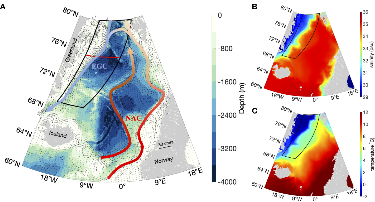
FIGURE1 Schematic of circulation (Raj et al., 2016; Våge et al., 2018; Huang et al., 2020) in the Nordic Sea and the study region (black boundaries). (A) Topography is from ETOPO1 (Amante and Eakins, 2009). The black arrows denote the 1993–2018 July climatological absolute geostrophic current field from AVISO. The thick red gradient lines present the North Atlantic Current, and the thick gray-blue line presents the East Greenland Current. The thin red line is the section selected for further analysis of spatial relationship between the main position of EGPF and the ice edge (15% sea ice concentration). (B) Spatial distributions of the July climatological sea surface salinity. (C) Spatial distributions of the July climatological sea surface temperature.

One of most conspicuous features of the Greenland Sea is the East Greenland Polar Front (EGPF), especially in the northern summer. EGPF is believed to have been formed by the interaction between Arctic-origin and Atlantic-origin water (Paquette et al., 1985; Kostianoy and Nihoul, 2009). In the Nordic Seas, EGPF exhibits a large gradient in terms of salinity and temperature fields (Figures 1B, C), whereas other fronts exhibit only a high salinity gradient, a high temperature gradient, or weak salinity and temperature gradients (Figures 2A, C). For example, the Norwegian Shelf Front has a high salinity gradient, and the Arctic Front and the Iceland Coastal Front have a high temperature gradient. Meanwhile, the Iceland-Faeroe Front has the characteristics of salinity and temperature fronts, but its gradients are weaker than those of EGPF (Figures 2A–D). With its high gradient of salinity and temperature, EGPF effectively separates Arctic-origin water from Atlantic-origin water.

FIGURE 2

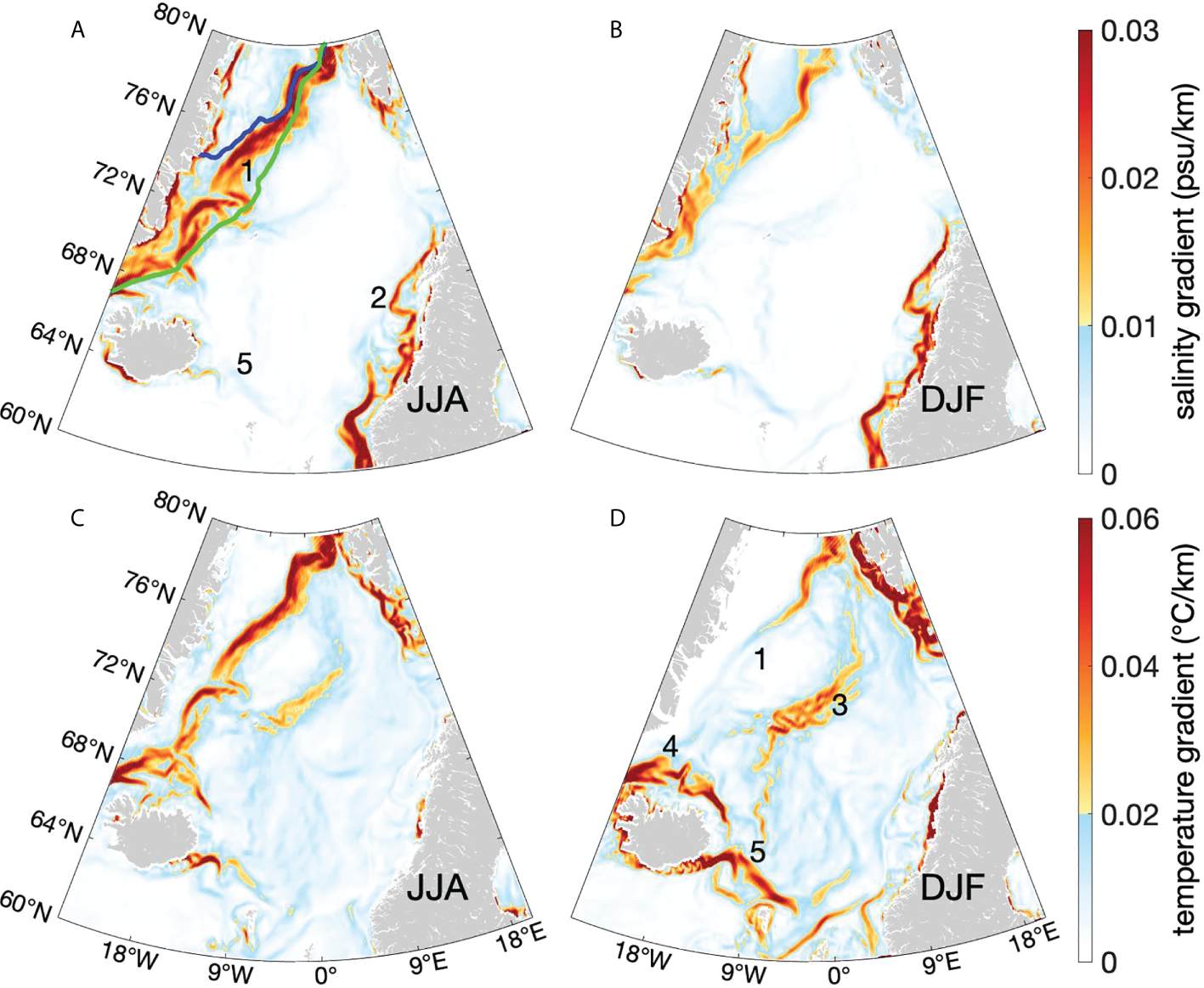
Figure 2 Spatial distributions of the horizontal gradient of (A) June to August (JJA) climatological average sea surface salinity, (B) December to February (DJF) climatological average sea surface salinity, (C) JJA climatological average sea surface temperature, and (D) DJF climatological average sea surface temperature. Numbers 1 to 5 in the figure represent the positions of (1) the East Greenland Polar Front, (2) the Norwegian Shelf Front, (3) the Arctic Front, (4) the Iceland Coastal Front, and (5) the Iceland–Faeroe Front. The green line is the median ice edge in February, and the blue line is the median ice edge in August (15% sea ice concentration).

Oceanic fronts can release potential energy to induce submesoscale motions (e.g., Manucharyan and Thompson, 2017). Therefore, they are thought to play a crucial role in the energy cascading from the global circulation scale to the small dissipation scale (Wadhams, 2005). In addition, the ocean front can affect the structure of the ocean flow field, ocean heat exchange, material transport, and air-sea interaction (Park and Chu, 2006). Various oceanic or atmospheric phenomena and processes—such as high biological productivity, abnormal wind and waves, dramatic changes in ocean color, strong vertical motion, and local weather conditions—are related to the ocean front (Vélez-Belchí and Tintoré, 2001; Sokolov and Rintoul, 2002; Nencioli et al., 2013). Large-scale fronts can influence the weather and even climate (Zhao et al., 2006). Some previous observational studies have demonstrated that the currents on both sides of the front differ considerably (Manley et al., 1987). The wind stress above the EGPF zone also changes rapidly (McPhee et al., 1987). Evidently, EGPF is an important ocean dynamic factor in the ocean–sea ice–atmosphere interactions in the Greenland Sea.

The sea ice in the Greenland Sea has been changing rapidly (Divine and Dick, 2006; Markus et al., 2009). According to a study that used the Pan-Arctic Ice Ocean Modeling and Assimilation System, from 1979 to 2016, the loss of the overall sea ice volume in the Greenland Sea was 113 km³ per decade (9.4 km³ month⁻¹ per decade) (Selyuzhenok et al., 2020). The ice conditions in the Greenland Sea are primarily regulated by the sea ice imported through the Fram Strait and by local sea ice variations (Selyuzhenok et al., 2020; Chatterjee et al., 2021). The sea ice area export shows considerable seasonal variations, with the maximum in March and the minimum in August (Smedsrud et al., 2017). The ice volume export presents a similar seasonal variation but has a relatively smaller February export in the freezing season (Min et al., 2019; Wei et al., 2019; Spreen et al., 2020). The sea ice volume export presents a notable decreasing trend due to the persistent thinning trend of Arctic sea ice (Wang et al., 2021). From 1992 to 2014, the Arctic Sea ice volume export displayed a negative trending with 27% ± 2% per decade (−54 ± 4 km³ month⁻¹ per decade) (Spreen et al., 2020). However, because of the increment in ice drift speed across 79°N, the annual ice area export has increased by about +6% per decade from 1979 (Smedsrud et al., 2017). The melting of sea ice exported from the Arctic basin through the Fram Strait dominates the freshwater content of Greenland open sea areas (de Steur et al., 2015).

Accompanying the fast-changing sea ice in the Greenland Sea, the subpolar Atlantic Meridional Overturning Circulation has been strengthening since the 2010s (Jackson et al., 2022). The flow strength of AW is largely controlled by the wind stress over the Greenland Sea (Muilwijk et al., 2019). The wind stress curl over the Greenland Sea presents a marked seasonal variation. It starts to build up in September, reaches its maximum in November, and maintains the maximum until April. Then, it almost disappears from May to August (Jónsson, 1991). The positive wind stress curl strengthens the cyclonic Greenland Sea Gyre (GSG) circulation in the central Greenland Sea. Warm and saline AW are recirculated from the FS region to the southwestern Greenland Sea by a strong GSG circulation (Chatterjee et al., 2021). The increase in temperature in AW along the main currents of the Nordic Seas induces an increase in the oceanic heat content in the Greenland Sea (Selyuzhenok et al., 2020).

Against the background of the freshening of the Arctic Ocean and warming of North AW, EGPF is hypothesized to exhibit significant variations in response to changes in the properties of Arctic-origin and Atlantic-origin water. Various oceanic or atmospheric phenomena and processes related to EGPF are expected to become increasingly vigorous. Studying the spatiotemporal variation of EGPF is one of fundamental tasks in this area.

Previous studies have shown that the position of the oceanic front is related to the ice edge location in the Pan-Arctic region (Niebauer and Alexander, 1985; Johannessen et al., 1987; Mu and Zhao, 2013; Strong and Rigor, 2013). According to a cruise observation in the Bering Sea in the Spring of 1982, the ice edge retreated by 6–38 cm/s from 1 to 12 May; the upper ocean front also moved fast and kept pace with the retreating ice edge, but the deeper front was nearly stationary (Niebauer and Alexander, 1985). Brenner et al. (2020) used an underway conductivity–temperature–depth system to capture the approximately 3-day evolution of a density front located at the ice edge in Beaufort Sea. They found that the frontogenesis in the marginal ice zone in Beaufort Sea is linked to an “up-front” wind stress. Our study area, East Greenland Sea, is far from Beaufort Sea. Although the oceanic fronts of both are in marginal ice zones, the sea ice conditions exhibit different spatial variations. In Beaufort Sea, the sea ice is over the salty water side across the fronts, and the melting is from the coastal sea to the open sea. In Greenland Sea, the sea ice is over the freshwater side across the fronts, and the melting is from the open sea to the continental shelf sea area.

The current study focuses on the variation region of EGPF. The study area is bounded by black curves in Figure 1 and is about 5.57 × 10⁵ km². We investigate the spatiotemporal variation of the EGPF in terms of seasonal cycles and long-term trend.

2 Data and methods

The horizontal gradients of the climatological sea surface salinity and climatological sea surface temperature in the Nordic Seas are not greater than 0.001 psu/km and 0.01°C/km, respectively (Kostianoy and Nihoul, 2009). He and Zhao (2011) examined the spatiotemporal variations of the oceanic front. They defined the salinity front threshold as 0.002 psu/km and the temperature front threshold as 0.015°C/km in the Nordic Seas to investigate the distribution characteristic of the front and its seasonal variation. The position and intensity of the front were defined using climatology and low-resolution data from a previous study. Notably, they analyzed EGPF at a depth of 100 m (He and Zhao, 2011). The main concern of our study is the near-surface layer that is directly affected by the sea ice. EGPF is a mesoscale process with rapidly spatiotemporal changes, especially in summer. Describing the intensity and position of surface EGPF by using daily high-resolution data and relative criteria for the defined front is reasonable. In this study, we utilize multi-year daily average reanalysis data to reshape EGPF by using reasonable thresholds. We employ the intensity and area in both surface and three-dimensional (3D) fields to describe EGPF. The seasonal variation and long-term trend of EGPF are investigated. We posit that the variation of the salinity characteristic of EGPF (salinity front) is directly affected by Arctic-origin water with the seasonal salinity variations modulated by sea ice. On the contrary, the variation of the temperature characteristic of EGPF (temperature front) is directly affected by Atlantic-origin water with seasonal temperature variations.

2.1 Data

Remote sensing data. Sea ice concentration and temperature data from the Operational Sea Surface Temperature and Ice Analysis (OSTIA)–reprocessed product (Good et al., 2020) are used in this study. These data have a horizontal resolution of 1/20°, and the time range is 1981–2020. The absolute geostrophic current data are from the Archiving, Validation, and Interpretation of Satellite Oceanographic Data (AVISO). These data have a horizontal resolution of 1/4° and spans the period of 1993–2019. All datasets are distributed by the Copernicus Marine Environment Monitoring Service (CMEMS; https://marine.copernicus.eu/).

Reanalysis data. For the salinity and temperature data, the global ocean eddy resolution reanalysis product called GLORYS12V1, which is also distributed by CMEMS, is used. GLORYS12 is a global eddy-resolving physical ocean and sea ice reanalysis with 1/12° horizontal resolution and 50 standard vertical levels. It covers the altimetry period of 1993 up to present. GLORYS12 assimilates along-track altimeter sea level anomaly, satellite sea surface temperature, sea ice concentration, and in situ temperature and salinity vertical profiles. Quality assessments have shown that GLORYS12 effectively captures the main, expected climate interannual variability signals for oceans and sea ice. It represents the small-scale variability of surface dynamics particularly well and effectively captures the low-frequency variability of the sea ice extent in Arctic and Antarctic Oceans (Jean-Michel et al., 2021). When assessed against 14 years (2002–2015) hydrographic observations collected at 59.5°N in the subpolar North Atlantic, the GLORYS12 effectively produced the thermohaline structure and reliably represented the ocean heat content in the upper 700-m layer (Verezemskaya et al., 2021). Further details about GLORYS12 can be obtained from the work of Jean-Michel et al. (2021).

2.2 Methods

2.2.1 Method for determining the front

Some studies have used the isoline of temperature, salinity, or density to determine the existence of a front (Van Aken et al., 1991; Parsons et al., 1996; Belkin and O'Reilly, 2009). This method is suitable for the frontal analysis of profile data. In this study, we use the front detection algorithm proposed by Belkin and O'Reilly (2009). The horizontal gradient field is calculated to determine the position and intensity of EGPF.

We calculate the distance between every two grid points as follows:

$\begin{array}{ll}dis=2arcsin\sqrt{{\sin }^2\frac{a}{2}+\cos \left(Lat1\right)\times \cos \left(Lat2\right)\times {\sin }^2\frac{b}{2}}\times R,& (1)\end{array}$

where a is the latitude difference Lat1− Lat2, b is the longitude difference Lon1 – Lon2, and R is the Earth’s radius (i.e., 6,378.137 km). Then, we use the Sobel operator’s convolution kernels GX and GY ( GX rotated by 90°) to calculate the gradients (GX, GY) in the X and Y directions, respectively. The calculation formula is as follows:

$\begin{array}{ll}\begin{array}{cc}GX=\left[\begin{array}{lll}-1\hfill & 0\hfill & 1\hfill \\ -2\hfill & 0\hfill & 2\hfill \\ -1\hfill & 0\hfill & 1\hfill \end{array}\right]& GY=\left[\begin{array}{lll}-1\hfill & -2\hfill & -1\hfill \\ 0\hfill & 0\hfill & 0\hfill \\ 1\hfill & 2\hfill & 1\hfill \end{array}\right]\\ G_x= \frac{1}{4}\ast GX\ast A/\left(2\ast di{s}_x\right)& G_y=\frac{1}{4}GY\ast A/\left(2\ast di{s}_y\right),\end{array}& (2)\end{array}$

where dis_x is the distance in the X direction between two grid points and dis_y is the distance in the Y direction. A is the original 2D data. Hence, the gradient value G can be obtained by the square root of the gradient in the X and Y directions as follows:

$\begin{array}{ll}G=\sqrt{G_x^2+G_y^2.}& (3)\end{array}$

The value of G is used to determine the position and intensity of EGPF. The threshold of the front is an empirical value and varies in different sea area. The selection of the threshold depends on the overall situation of the spatial and temporal characteristics of the front in the study area. If the threshold is set too low, then the sea area will be full of fronts. If the threshold is set too high, then fronts will no longer be continuous spatially and temporally. In this study, we choose 0.04 psu/km and 0.09°C/km as the threshold value of salinity and temperature fronts to define the daily EGPF. These thresholds satisfy the continuity conditions in space and time. In the probability cumulative curve of the gradient values in the research area, these thresholds correspond to about 95% of the accumulation grid points (non-front area; Figures 3A, B). These thresholds can avoid the disorder of fronts in the study area. The climatological gradient values are the mean of daily gradient values. We choose 0.01 psu/km and 0.02°C/km as the threshold values to define the climatological EGPF in the Greenland Sea. The area of the climatological EGPF is larger than the daily EGPF, so the climatological EGPF thresholds correspond to about 85% of the accumulation grid points (non-front area; Figures 3C, D) in the research area.

FIGURE 3

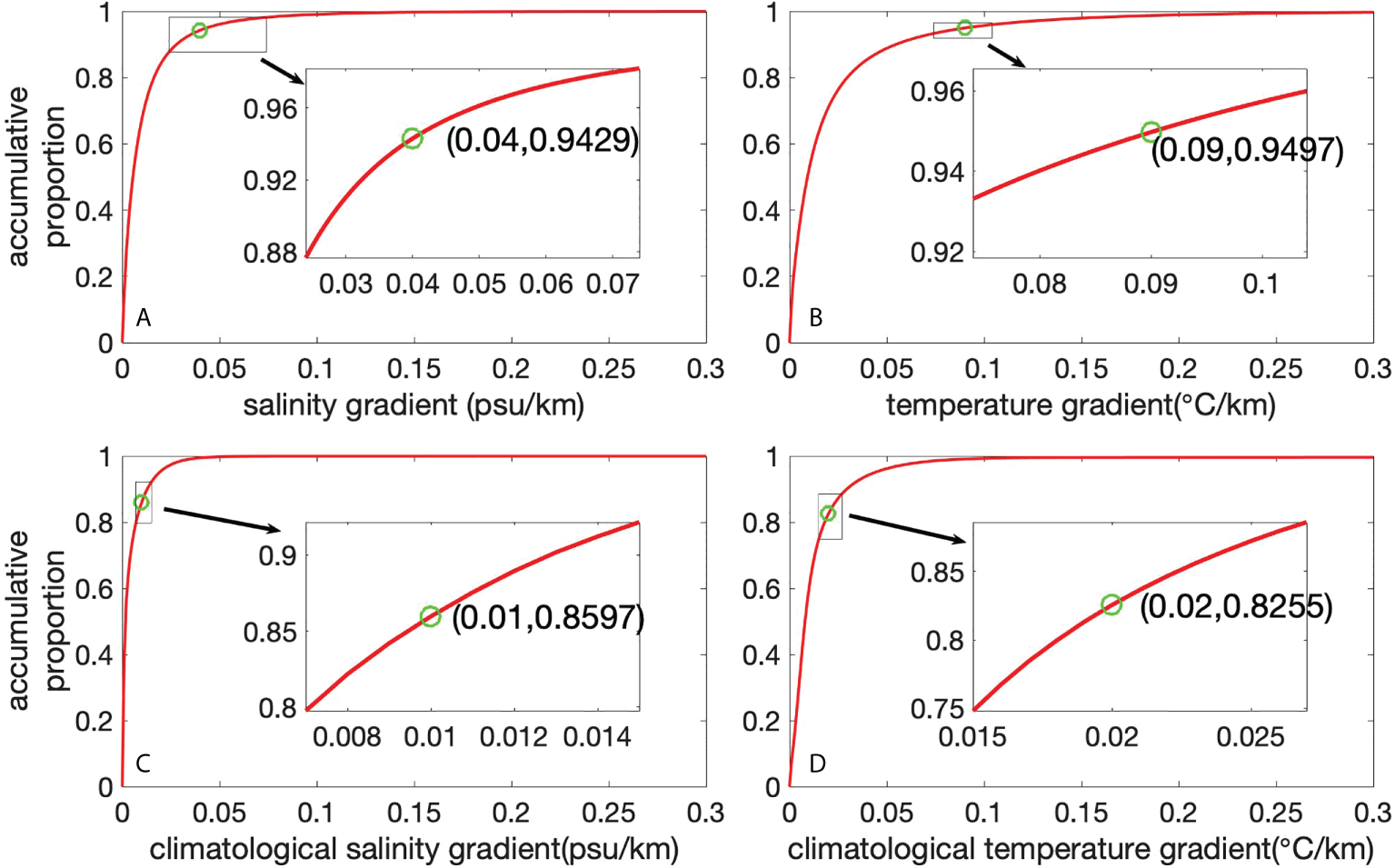
Figure 3 Thresholds. Grid point number accumulative curves of (A) 1993–2018 salinity gradient, (B) 1993–2018 temperature gradient, (C) climatological salinity gradient, and (D) climatological temperature gradient.

2.2.2 Surface characteristic of the front

We use two indices, the front area and the mean intensity, to describe EGPF. The front area S_g of the front is calculated as follows:

$\begin{array}{ll}\begin{array}{c}{S}_i=di{s}_{xi}*di{s}_{yi}\\ S={\displaystyle \sum _{i=1}^n{G}_{mask}\times S_i,}\end{array}& (4)\end{array}$

where dis_xi and dis_yi are the distances between two adjacent grid points in the zonal and meridional directions, respectively; S_i is the grid area; and G_mask is a matrix, in which the part corresponding to G being greater than the threshold value is set to 1, and the rest is set to 0. The average intensity of the front is defined as follows:

$\begin{array}{ll}\overline{G}=\frac{{\displaystyle {\sum }_{i=1}^n{G}_{mask}\times G_i\times S_i}}{{\displaystyle {\sum }_{i=1}^n{G}_{mask}\times S_i}}.& (5)\end{array}$

The front area calculation method shown above is affected by the resolution of the data grid, but the average intensity is not. In this study, we use the average intensity and front area to analyze the variation of the EGPF in the Greenland Sea.

2.2.3 3D characteristics of the front

Similar to the surface characteristics, we use the front volume and the 3D mean intensity to describe EGPF. The volume of EGPF is defined as follows:

$\begin{array}{ll}V={\displaystyle \sum _{k=1}^h{\displaystyle \sum _{i=1}^n{S}_{i,k}\times h_k\times G_{mask,k}.}}& (6)\end{array}$

where hk is the layer thickness and k is the layer index. GLORYS12 has 50 vertical levels. The level depth is the center depth of the associated layer. The seasonal variation of the front (strength) is mainly in the upper 19 levels. We select the upper 19 layers to calculate the front volume. We multiple the front area by the layer thickness in each layer and then integrate the vertical volume. The integrated thickness is actually about 60 m (60.3 m).

The mean 3D front intensity is defined as follows:

$\begin{array}{ll}\overline{G_{3D}}=\frac{{\displaystyle {\sum }_{k=1}^h{\displaystyle {\sum }_{i=1}^n{G}_{i,k}\times S_{i,k}\times h_k\times G_{mask,k}}}}{V}& (7)\end{array}$

We multiply the gradient by its 3D grid volume and then average the total value of the whole volume.

2.2.4 Heat content transport

The heat content transport along one section is calculated as follows:

$\begin{array}{ll}\begin{array}{c}{S}_i=di{s}_{xi}\ast h_k\\ Q_t={\rho }_0{c}_p{\displaystyle \sum _{i=1}^n{T}_{i,k}\times S_i\times V_{i,k},}\end{array}& (8)\end{array}$

where Q_t is the heat content transport, S_i is the grid area, dis_xi is the distance between two adjacent grid points in the zone, h_k is the vertical layer thickness, ρ₀ is sea water density, c_p is the sea water specific heat capacity, T_i,k is the temperature at each point in each layer, and V_i,k is the southward velocity at each point in each layer.

The seasonal temperature variations change obviously in the upper 14 levels. We calculate the heat content transport in the upper 14 layers along the red line section in Figure 1A. The integrated thickness is actually about 30 m (29.447 m).

3 Results

3.1 Spatial relationship between the main position of the EGPF and the ice edge

As the sea ice melts in the Greenland Sea from June to September, the sea ice extent shrinks toward the continental shelf, and EGPF moves and keeps pace with the ice edge. The spatial distributions of the ice edge and the horizontal gradient of the sea surface salinity/sea surface temperature in the Greenland Sea on 18 June and 18 July 2012 are shown in Figure 4. The black line is the daily marginal ice line, and the purple line is the 330-m isobath and represents the shelf break with a high topography gradient between the continental shelf and the slope. On 18 June 2012 (Figures 4A, C), the ice edge was located outside the shelf break. Its southernmost point reached 67°N, and the overall sea ice extent shrank toward high latitudes. On 18 July 2012 (Figures 4B, D), the ice edge was near the continental shelf break, and its southernmost point was at 69°N. In most years, the sea ice covered the continental shelf north of 77°N. Compared with the situation in 2012, the ice edge in the other years presented a similar variation, but the sea ice extent shrank more significantly.

FIGURE 4

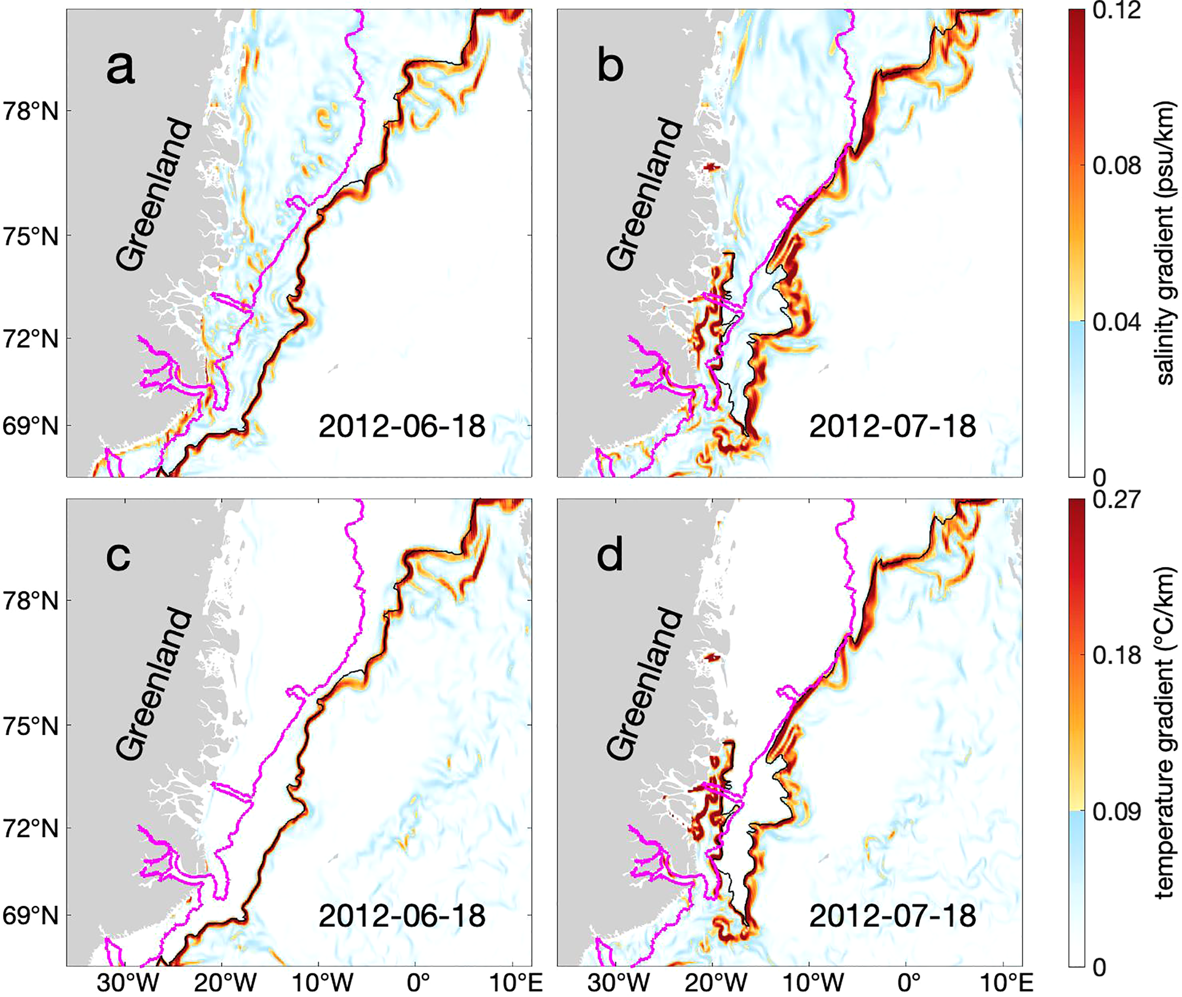
Figure 4 Spatial distributions of the ice edge, salinity front, and temperature front in the Greenland Sea on 18 June and 18 July 2012. (A, B) Horizontal gradient of sea surface salinity and (C, D) horizontal gradient of sea surface temperature. The black line is the daily ice edge, and the purple line is the 330-m isobath that represents the shelf break with a high topography gradient.

When the ice edge is outside the shelf break (Figures 4A, C), the strong salinity and temperature gradient is mainly concentrated at the ice edge. During the northward movement of the south margin of the ice edge, the front moves and keeps pace with the ice edge. When the sea ice retreats toward the continental shelf, the front is limited to the shelf break (Figures 4B, D), but the intensity and area of the front gradually decrease after the sea ice shrinks further more (not shown).

To clarify the relationship between the position of the EGPF and the ice edge in the Greenland Sea, we select a section (red line in Figure 1A) to analyze the relative position changes compared with the shelf-slope break. The daily variations of the sea surface salinity horizontal gradient and sea surface temperature horizontal gradient along the section in 2004 are shown in Figure 5. The results are similar for the other years (not shown). The black dots are the daily variation of the intersections between the marginal ice line and the section line, and the solid purple line is the position of the shelf break along the section line (Figures 5A, B). In May, the sea ice area (concentration and extent) begins to decline, the seawater under the ice is freshened, and a strong gradient appears. In June, the intensity of EGPF strengthens. When the sea ice is beyond the continental shelf from June to August, EGPF is always distributed along the ice edge and keeps pace with the ice edge. When the sea ice shrinks back to the continental shelf (black dots below the solid purple line), EGPF is restricted to the vicinity of the shelf break. However, its intensity is gradually reduced. After August, EGPF (salinity front and temperature fronts) gradually weakens.

FIGURE 5

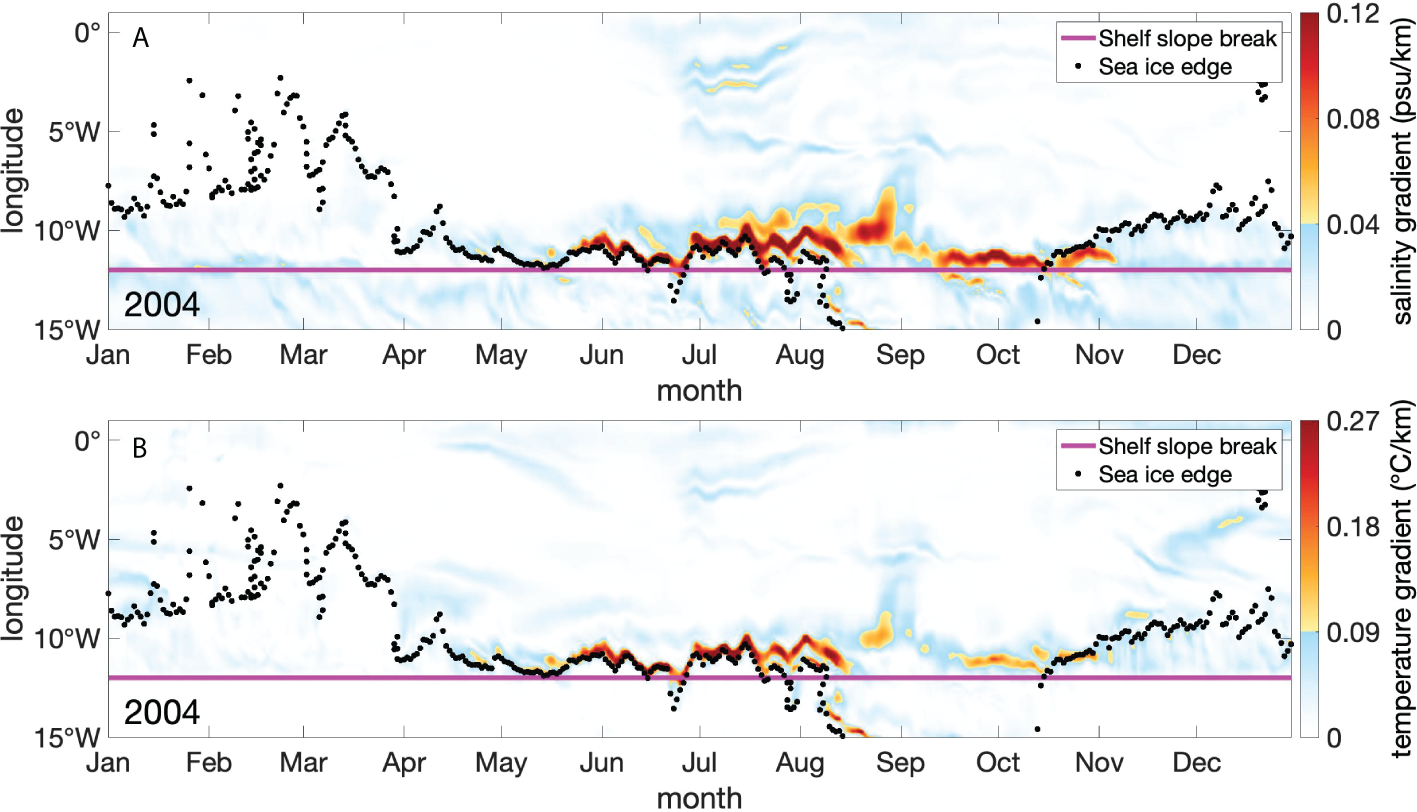
Figure 5 Daily variation of (A) sea surface salinity horizontal gradient and (B) sea surface temperature horizontal gradient (background color) along the section (red line) indicated in Figure 1A. The black dots are the daily variation of the intersections between the marginal ice line and the section line. The abscissa is the time for 2004, and the ordinate is the longitude of the section. The solid purple line is the position of the shelf break along the section line.

3.2 Seasonal variations of EGPF

On the basis of observed/reanalysis data, the climatological (1993–2018) seasonal variation in the study area (thick black solid and dashed lines in Figure 6A) shows that the sea ice area decreases rapidly in May, shrinks to the continental shelf sea area in July (the continental shelf sea area of the research area is about 9.53 × 10⁴ km², marked with a thin solid black line in Figure 6A), and reaches its minimum value of 2.86 × 10⁴ km²/3.07 × 10⁴ km² in September. The sea ice area accounts for about 5%–5.5% of the total study area (5.57 × 10⁵ km²). Notably, this conclusion is based on climatological statistical results. It varies slightly in some local regions in some years. For example, in Figure 5, the sea ice edge (15% sea ice concentration) with a strong front is not within the shelf slope break sea area in early August due to the complex sea ice conditions and topography influence. However, generally, the sea ice retreats from the southeast outer shelf to the northwest shelf in summer and shrinks to the continental shelf sea area in the southern part of the study area in July.

FIGURE 6

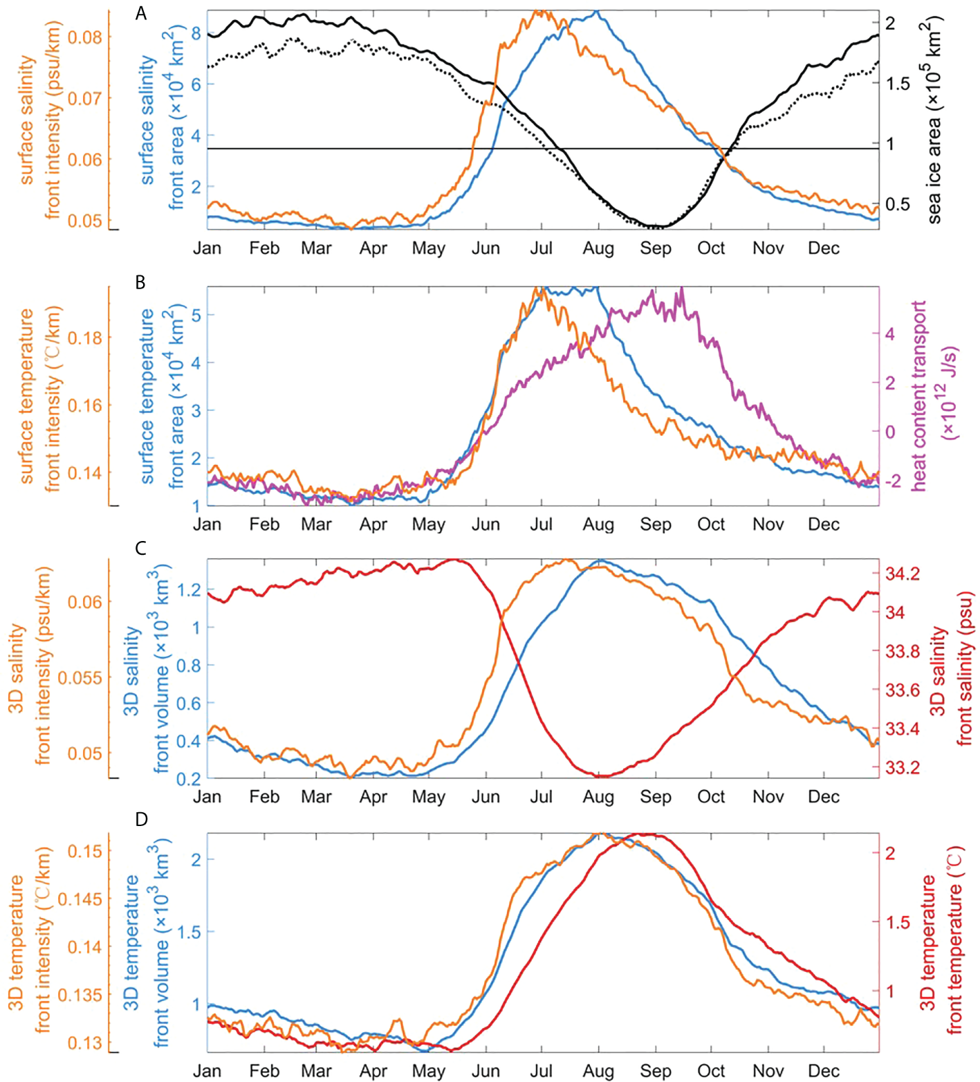
Figure 6 Seasonal variations. (A) Surface salinity front intensity, area and sea ice area. The thick black solid/dashed line refers to the GLORYS12v1/remote sensing data results. The thin solid black line represents the continental shelf area of the research area. (B) Surface temperature front intensity, area, and heat content transport along the upper 25-m section (red line) indicated in Figure 1A. (C) 3D salinity front intensity, volume, and averaged salinity. (D) The 3D temperature front intensity, volume, and averaged temperature.

We use four indicator variables, namely, surface front area, surface front intensity, 3D front volume, and the 3D front intensity, to explore the variation of the EGPF. The salinity and temperature fronts do not fully overlap spatially, and they have different characteristics and temporal variations. We discuss them separately. In the analysis, the daily thresholds of the salinity front and the temperature front are set to 0.04 psu/km and 0.09°C/km, respectively.

With regard to the climatological seasonal variation, the surface salinity front intensity and front area (Figure 6A) begin to increase rapidly in May. The surface salinity front intensity reaches its highest value of 0.08 psu/km in the early July and the salinity front area reaches its peak value of 8.86 × 10⁴ km² (the area proportion is about 16%) at the end of July. Although the sea ice continues to melt until September, when the sea ice shrinks back to the continental shelf, EGPF is limited to the continental shelf break. As the thermodynamic environment for maintaining EGPF disappears, the EGPF’s intensity begins to decrease. However, because of mixing and diffusion, the EGPF area can enlarge and reach its peak in August. After August, the intensity and area of the EGPF gradually weaken until April of the next year.

The intensity of the surface temperature front (Figure 6B) has a similar seasonal variation as the salinity front intensity. It also reaches its highest value of 0.19°C/km in July and then decreases. However, the temperature front area is different from the salinity front area. The area of the temperature front reaches its peak value of 5.58 × 10⁴ km² (the area proportion is about 10%) in early July and then maintains this peak value in the whole of July. After August, the temperature front area gradually reduces with intensity. The heat content transport along the upper 25-m section begins to increase rapidly in May (Figure 6B). It reaches its peak value of 5.84 × 10¹²J/s in the middle of September and then decreases. In a previous study by He and Zhao (2011), a strong and continuous temperature front was observed in September. We think the different result is mainly due to the depth used for analysis. We study EGPF in the surface ocean which is close to the variation of sea ice, whereas they analyzed the front at a depth of 100 m.

As the sea ice melts in summer, the extent of the fresh water expands and deepens, and the salinity gradient gradually strengthens. The climatological evolution processes are shown by the variations of the red isolines for salinity and dashed isolines for the salinity gradient in Figures 7A–D. The gradient isolines are larger than the climatological threshold of 0.01 psu/km. The 3D daily characteristics are mainly reflected in the upper 55 m. The spatial distributions of the horizontal gradient of salinity at 0, 47, and 92 m depths on 6 August 1993 are shown in Figure 8. The daily threshold of the salinity front is still set to 0.04 psu/km. We select the salinity/temperature front in the upper 55 m for a 3D daily analysis.

FIGURE 7

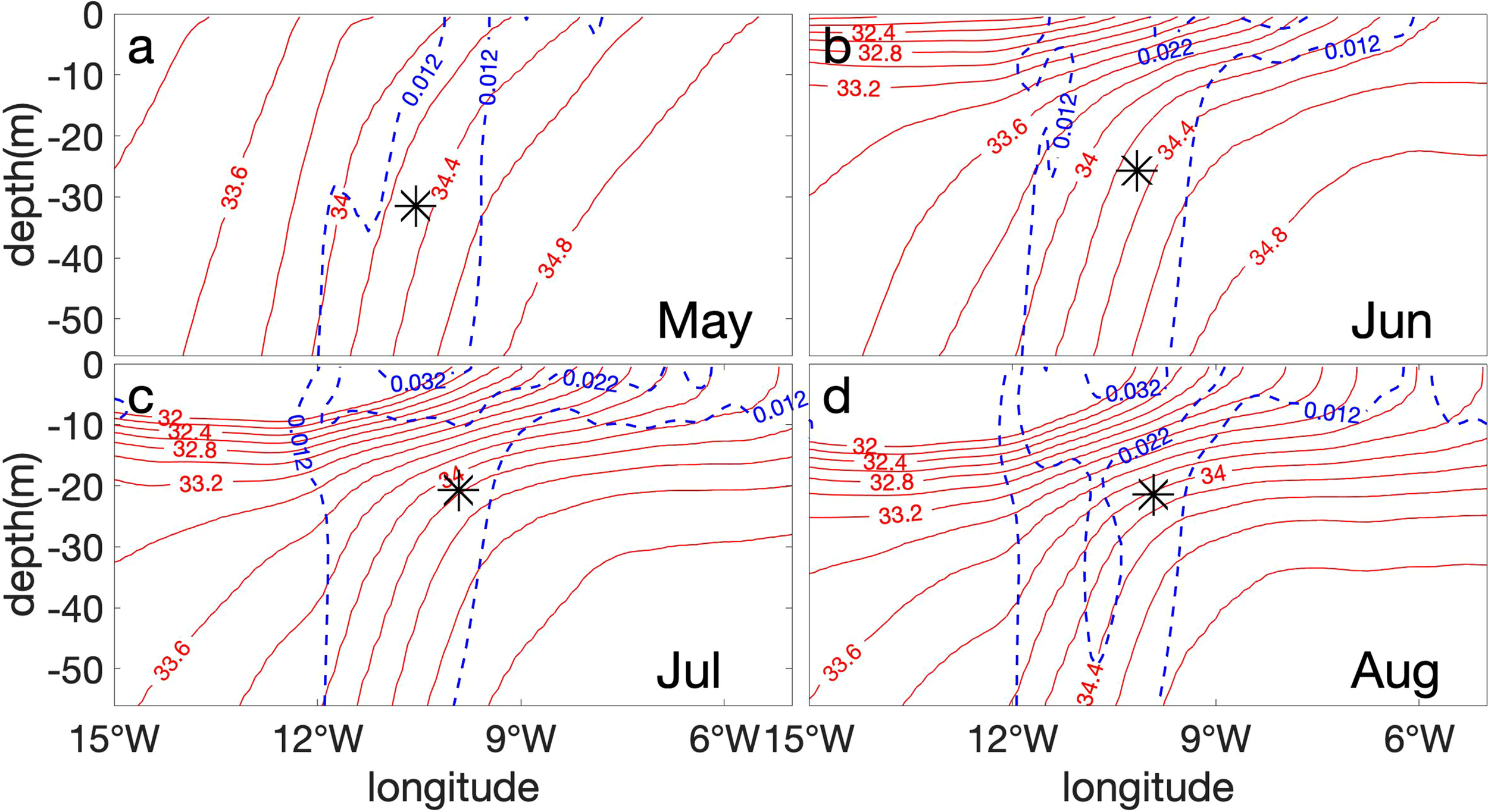
Figure 7 Climatological monthly salinity and salinity gradient along the red line section in Figure 1A (A–D for May to August). The red solid lines are the salinity isolines, the blue dashed lines are the salinity gradient isolines, and the black marks represent the centers of the salinity front in the upper 55-m section.

FIGURE 8

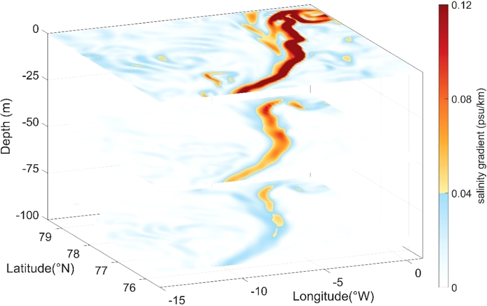
Figure 8 The spatial distributions of the horizontal gradient of the salinity in 0, 47, and 92 m on 6 August 1993.

With regard to the climatological seasonal variation (Figure 6C), the 3D salinity front intensity and volume also increases rapidly in May. The 3D intensity reaches its peak value of 0.06 psu/km in the middle of July and then decreases. Compared with the surface intensity peak, there is a time lag of about half a month. The 3D volume reaches its peak value of 1.35 × 10³ km³ at the end of July, and the volume proportion is about 4% compared with the whole volume of 3.36 × 10⁴ km³ of the research region. In addition, with sea water desalination, the salinity of the 3D salinity front decreases rapidly in May. It drops from the maximum value of 34.27 psu to the minimum value of 33.15 psu at the end of July.

Compared with the salinity front, the intensity and volume of the 3D temperature front reach the peak value of 0.15°C/km and 2.18 × 10³ km³, respectively (the volume proportion is about 6.5%), at the end of July (Figure 6D) and then decreases. The background temperature reaches its peak value of 2.14°C at the end of August.

3.3 Long-term trend of EGPF

Sea ice has been decreasing considerably in recent decades. According to analyses based on satellite passive microwave radiometers, the sea ice extent trend was −6.5 ± 1.1 × 10³ km²/year (−8.6 ± 1.5% decade⁻¹) in the Greenland Sea from 1979 to 2010 (Cavalieri and Parkinson, 2012). According to GLORYS12V1 (1993–2018), in our study area, the sea ice area anomaly presented an increasing trend from 1993 to 1997, and a decreasing trend from 1998 to 2018. According to Cavalieri’s results, the ice area of the Greenland Sea also showed this decadal regime shift around 1997 (Cavalieri and Parkinson, 2012). In this study, we mainly analyze the sea ice and EGPF from 1998 to 2018.

The long-term trend of the monthly sea ice area anomaly obtained after subtracting the climatological monthly mean is shown in Figure 9A. It presented a decreasing trend of −1.66 × 10³ km²/year (−1.57 × 10³ km²/year in remote sensing data; both significant at the 95% confidence level) from 1998 to 2018. Across the thin red line in Figure 1A, the monthly heat content transport anomaly presented an increasing trend of 3.72 × 10¹⁰ J/s/year from 1998 to 2018 (Figure 10A; statistically significant at the 95% confidence level).

FIGURE 9

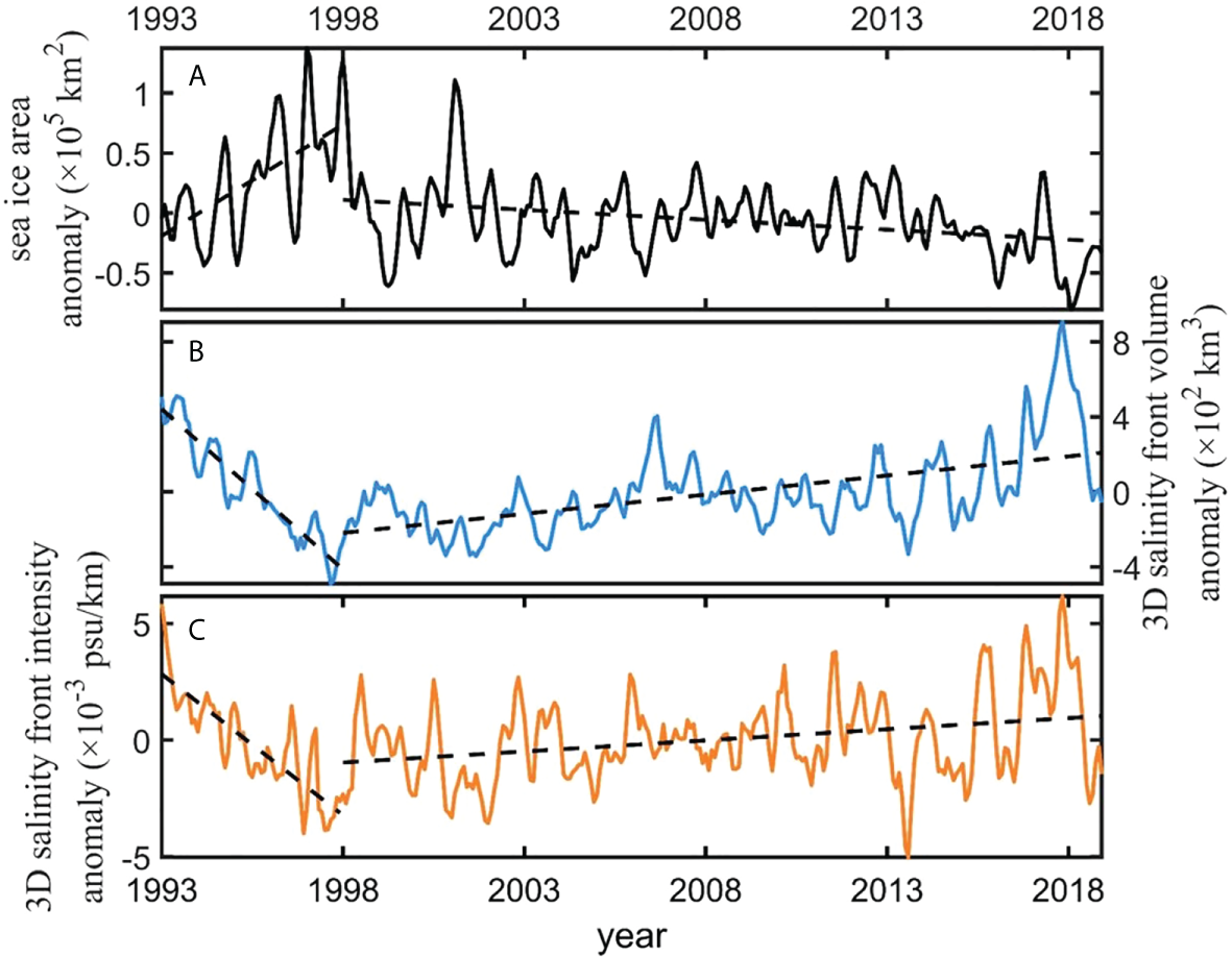
Figure 9 Long-term trend from GLORYS12v1 data. (A) Monthly sea ice area anomaly, (B) 3D salinity front volume anomaly, and (C) intensity anomaly. All lines are filtered by three (months) points moving average.

FIGURE 10

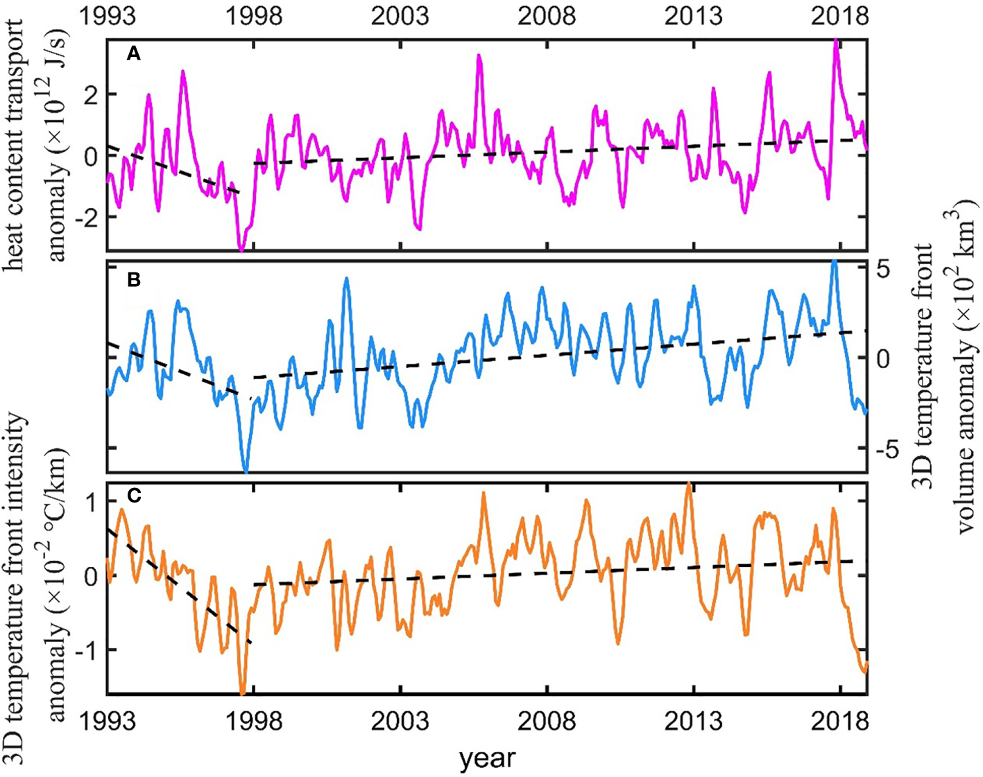
Figure 10 Long-term trend. (A) Monthly heat content transport anomaly along the upper 25-m section (red line) indicated in Figure 1A, (B) 3D temperature front volume anomaly, and (C) intensity anomaly. All lines are filtered by three (months) points moving average.

Given this background, the monthly 3D salinity front volume anomaly showed an increasing trend of 20.41 km³/year from 1998 to 2018 (Figure 9B; statistically significant at the 95% confidence level). The monthly 3D salinity front intensity anomaly presented an increasing trend of 9.56 × 10⁻⁵ psu/km/year from 1998 to 2018 (Figure 9C; statistically significant at the 95% confidence level). The 21-year increasing value 2.01 × 10⁻³ psu/km could reach about 5% (20%) of the daily threshold of 0.04 psu/km (climatological threshold of 0.01 psu/km). The intensity and volume show that the salinity front gradually strengthened in recent years.

The long-term trend of the 3D temperature front is shown in Figure 10. The monthly volume anomaly of the temperature front increased by 12.29 km³/year from 1998 to 2018 (Figure 10B; statistically significant at the 95% confidence level). The monthly temperature front intensity anomaly increased by 1.55 × 10⁻⁴°C/km/year from 1998 to 2018 (Figure 10C; statistically significant at the 95% confidence level), The total increase could be up to 3.6% (16%) of the daily threshold of 0.09°C/km (climatological threshold of 0.02°C/km). The temperature front also gradually strengthened in recent years.

4 Discussion and conclusion

The spatiotemporal variations of 3D daily EGPF are analyzed on the basis of GLORYS12V1 reanalysis data from 1993 to 2018. The significant spatial relationship between the main position of EGPF and the position of the marginal ice edge before the sea ice shrinks to the shelf break is illustrated. In summer, the solar shortwave radiation increases, leading to a rise in air and seawater temperature. As the sea ice melts dramatically, the cold and fresh seawater induces and strengthens the salinity and temperature fronts. Thus, the front area with strong salinity and temperature gradients is mainly distributed along the ice edge.

Affected by the formation and melting of sea ice, the intensity and area of EGPF (salinity front) show seasonal variations. The sea ice area begins to decrease rapidly in May, whereas the average intensity and area of the salinity front begin to increase rapidly. When the sea ice extent shrinks to the continental shelf in late June, the surface intensity of the salinity front reaches its highest value (~0.08 psu/km). The sea ice continues to melt in the continental shelf, and the front is restricted to the continental shelf break. In the meantime, the maintaining mechanism of the strong salinity gradient steadily weakens in the shelf break, and the salinity front intensity begins to decrease. Although the front intensity weakens due to the horizontal diffusion and mixing, the surface salinity front area is still expands and reaches its peak value of ~8.86 × 10⁴ km² (16% of the research area) in late July. Then, the salinity front area gradually decreases. The variation of EGPF (temperature front) is directly affected by Atlantic-origin water, and this front also shows seasonal variations. The surface temperature front’s intensity and front area begin to increase rapidly in May. The intensity of the surface temperature front reaches its highest value of 0.19°C/km in July and then decreases. The temperature front area reaches its peak value of 5.58 × 10⁴ km² (the area proportion is about 10%) in early July and then maintains this peak value in the whole of July. After August, the temperature front area gradually decreases with intensity. The heat content transport along the upper 25-m section begins to increase rapidly in May. It reaches its peak value 5.84 × 10¹²J/s in the middle of September and then decreases.

Compared with the surface, although the 3D salinity/temperature front intensity and volume also increases rapidly in May, there is a time lag before 3D intensity reaches the peak value. The 3D salinity front intensity reaches its peak value of 0.06 psu/km in the middle of July. The 3D temperature front reaches its peak value of 0.15°C/km at the end of July. In the upper 55 m, the research volume is about 3.36 × 10⁴ km³. The 3D salinity front volume reaches its peak value of 1.35 × 10³ km³ (the volume proportion is 4% compared with the research volume) at the end of July, and the 3D temperature front volume reaches its peak value of 2.18 × 10³ km³ (6.5%).

In terms of long-term trend, the EGPF gradually strengthens as the sea ice area decreases. Specifically, from 1998 to 2018, the sea ice area showed a decreasing trend of −1.66 × 10³ km²/year in the Greenland Sea. The melting of sea ice increases year by year in summer. Given this background, the 3D salinity front intensity increases by 9.56 × 10⁻⁵ psu/km/year, and the total (21 years) increase is about 5% (20%) of the daily (climatological) threshold. The salinity front volume shows an increasing trend of 20.41 km³/year. The heat content transport anomaly increases by 3.72 × 10¹⁰ J/s/year. The 3D temperature front intensity has an increasing trend of 1.55 × 10⁻⁴°C/km/year, and the total increase is about 3.6% (16%) of the daily (climatological) threshold. The 3D temperature front volume also has an increasing trend of 12.29 km³/year.

Given the freshening of the Arctic Ocean and warming of North AW, the strength and range of EGPF show increasing trends. As the transition zone, EGPF presents high contrast between Arctic-origin and Atlantic-origin water. The strengthening of EGPF induces abundant energetic submesoscale motions. In the Greenland Sea, the early (delayed) spring phytoplankton bloom associated with high primary production levels is linked to high (low) Arctic sea ice flux through the Fram Strait (Mayot et al., 2020). Given the strong convergence ability of EGPF, the variations of EGPF influence the chlorophyll-a and phytoplankton distributions and variations in the Greenland Sea. We can speculate that various oceanic or atmospheric phenomena and processes related to EGPF will become increasingly active. Furthermore, the frontal process is closely related to mixing. One of the front generation mechanisms is shear dispersion. Oscillation wind induces spatial inhomogeneity in the horizontal mixing, and the minimum total diffusivity is accompanied with the maximum property gradient. The wind-induced shear dispersion facilitates the frontogeneses in the shelf break (Ou and Chen, 2006). Meanwhile, rapid cross-frontal mixing is generated by frontal instabilities (Wenegrat et al., 2020). The Greenland Sea is one of the important sea areas affecting the North Atlantic thermohaline circulation through mixing. Thus, further study of the dynamic processes associated with EGPF throughout its various stage is necessary.

Data availability statement

The original contributions presented in the study are included in the article/Supplementary Material. Further inquiries can be directed to the corresponding author.

Author contributions

YL initiated the idea, designed the study. YL, JW and GH analyzed the data and contributed to the writing of the manuscript. GH, XL, GY, and QJ revised and edited the manuscript. All authors contributed to the article and approved the submitted version.

Funding

This study was supported by the National Key Research and Development Program of China (2018YFA0605904); the Innovation Group Project of Southern Marine Science and Engineering Guangdong Laboratory (Zhuhai) (311020004 and SML2020SP007); the Natural Science Foundation of China project (41806030 and 41806004).

Conflict of interest

The authors declare that the research was conducted in the absence of any commercial or financial relationships that could be construed as a potential conflict of interest.

Publisher’s note

All claims expressed in this article are solely those of the authors and do not necessarily represent those of their affiliated organizations, or those of the publisher, the editors and the reviewers. Any product that may be evaluated in this article, or claim that may be made by its manufacturer, is not guaranteed or endorsed by the publisher.

References

Amante C., Eakins B. W. (2009). “ETOPO1 1 arc-minute global relief model: Procedures, data sources and analysis,” in NOAA Technical memorandum NESDIS NGDC-24 (National Geophysical Data Center, NOAA, Boulder, Colorado). doi: 10.7289/V5C8276M

CrossRef Full Text | Google Scholar

Ballinger T. J., Hanna E., Hall R. J., Miller J., Ribergaard M. H., Høyer J. L., et al. (2018). Greenland Coastal air temperatures linked to Baffin bay and Greenland Sea ice conditions during autumn through regional blocking patterns. Climate Dynam. 50 (1), 83–100. doi: 10.1007/s00382-017-3583-3

CrossRef Full Text | Google Scholar

Belkin I. M., O'Reilly J. E. (2009). An algorithm for oceanic front detection in chlorophyll and SST satellite imagery. J. Mar. Syst. 78 (3), 319–326. doi: 10.1016/j.jmarsys.2008.11.018

CrossRef Full Text | Google Scholar

Brenner S., Rainville L., Thomson J., Lee C. (2020). The evolution of a shallow front in the Arctic marginal ice zone. Elementa.: Sci. Anthropocene. 8 (1), 17. doi: 10.1525/elementa.413

CrossRef Full Text | Google Scholar

Cavalieri D. J., Parkinson C. L. (2012). Arctic Sea ice variability and trend 1979–2010. Cryosphere. 6 (4), 881–889. doi: 10.5194/tc-6-881-2012

CrossRef Full Text | Google Scholar

Chatterjee S., Raj R. P., Bertino L., Mernild S. H., Subeesh M. P., Murukesh N., et al. (2021). Combined influence of oceanic and atmospheric circulations on Greenland sea ice concentration. Cryosphere. 15 (3), 1307–1319. doi: 10.5194/tc-15-1307-2021

CrossRef Full Text | Google Scholar

de Steur L., Pickart R. S., Torres D. J., Valdimarsson H. (2015). Recent changes in the freshwater composition east of Greenland. Geophys. Res. Lett. 42 (7), 2326–2332. doi: 10.1002/2014GL062759

CrossRef Full Text | Google Scholar

Divine D. V., Dick C. (2006). Historical variability of sea ice edge position in the Nordic seas. J. Geophys. Res.: Ocean. 111, C010011. doi: 10.01029/02004JC002851

CrossRef Full Text | Google Scholar

Good S., Fiedler E., Mao C., Martin M. J., Maycock A., Reid R., et al. (2020). The current configuration of the OSTIA system for operational production of foundation sea surface temperature and ice con-centration analyses. Remote Sens 12(4), 720. doi: 10.3390/rs12040720

CrossRef Full Text | Google Scholar

Håvik L., Pickart R. S., Våge K., Torres D., Thurnherr A. M., Beszczynska-Möller A., et al. (2017). Evolution of the East Greenland current from fram strait to Denmark strait: Synoptic measurements from summer 2012. J. Geophys. Res.: Ocean. 122 (3), 1974–1994. doi: 10.1002/2016JC012228

CrossRef Full Text | Google Scholar

He Y., Zhao J. (2011). Distributions and seasonal variations of fronts in GIN seas. Adv. Earth Sci. 26 (10), 1079–1091. doi: 10.11867/j.issn.1001-8166.2011.10.1079

CrossRef Full Text | Google Scholar

Huang J., Pickart R. S., Huang R. X., Lin P., Brakstad A., Xu F., et al. (2020). Sources and upstream pathways of the densest overflow water in the Nordic seas. Nat. Commun. 11 (1), 1–9. doi: 10.1038/s41467-020-19050-y

PubMed Abstract | CrossRef Full Text | Google Scholar

Jackson L. C., Biastoch A., Buckley M. W., Desbruyères D. G., Frajka-Williams E., Moat B., et al. (2022). The evolution of the north Atlantic meridional overturning circulation since 1980. Nat. Rev. Earth Environ. 3 (4), 241–254. doi: 10.1038/s43017-022-00263-2

CrossRef Full Text | Google Scholar

Jean-Michel L., Eric G., Romain B.-B., Gilles G., Angélique M., Marie D., et al. (2021). The Copernicus global 1/12° oceanic and Sea ice GLORYS12 reanalysis. Front. Earth Sci. 9. doi: 10.3389/feart.2021.698876

CrossRef Full Text | Google Scholar

Johannessen J., Johannessen O., Svendsen E., Shuchman R., Manley T., Campbell W. J., et al. (1987). Mesoscale eddies in the fram strait marginal ice zone during the 1983 and 1984 marginal ice zone experiments. J. Geophys. Res.: Ocean. 92 (C7), 6754–6772. doi: 10.1029/JC092iC07p06754

CrossRef Full Text | Google Scholar

Jónsson S. (1991). Seasonal and interannual variability of wind stress curl over the Nordic seas. J. Geophys. Res.: Ocean. 96 (C2), 2649–2659. doi: 10.1029/90JC02230

CrossRef Full Text | Google Scholar

Kostianoy A. G., Nihoul J. C. J. (2009). “Frontal zones in the Norwegian, Greenland, barents and Bering seas,” in Influence of climate change on the changing Arctic and Sub-Arctic conditions. Eds. Nihoul J. C. J., Kostianoy A. G. (Dordrecht: Springer), 171–190.

Google Scholar

Li C., Battisti D. S., Schrag D. P., Tziperman E. (2005). Abrupt climate shifts in Greenland due to displacements of the sea ice edge. Geophys. Res. Lett. 32 (19), L19702. doi: 10.1029/2005GL023492

CrossRef Full Text | Google Scholar

Manley T., Hunkins K., Muench R. (1987). Current regimes across the East Greenland polar front at 78° 40′ north latitude during summer 1984. J. Geophys. Res.: Ocean. 92 (C7), 6741–6753. doi: 10.1029/JC092iC07p06741

CrossRef Full Text | Google Scholar

Manucharyan G. E., Thompson A. F. (2017). Submesoscale sea ice-ocean interactions in marginal ice zones. J. Geophys. Res.: Ocean. 122 (12), 9455–9475. doi: 10.1002/2017JC012895

CrossRef Full Text | Google Scholar

Markus T., Stroeve J. C., Miller J. (2009). Recent changes in Arctic sea ice melt onset, freezeup, and melt season length. J. Geophys. Res.: Ocean. 114 (C12), C12024. doi: 10.1029/2009JC005436

CrossRef Full Text | Google Scholar

Mayot N., Matrai P. A., Arjona A., Bélanger S., Marchese C., Jaegler T., et al. (2020). Springtime export of Arctic sea ice influences phytoplankton production in the Greenland Sea. J. Geophys. Res.: Ocean. 125 (3), e2019JC015799. doi: 10.1029/2019JC015799

CrossRef Full Text | Google Scholar

McPhee M. G., Maykut G. A., Morison J. H. (1987). Dynamics and thermodynamics of the ice/upper ocean system in the marginal ice zone of the Greenland Sea. J. Geophys. Res.: Ocean. 92 (C7), 7017–7031. doi: 10.1029/JC092iC07p07017

CrossRef Full Text | Google Scholar

Min C., Mu L., Yang Q., Ricker R., Shi Q., Han B., et al. (2019). Sea Ice export through the fram strait derived from a combined model and satellite data set. Cryosphere. 13 (12), 3209–3224. doi: 10.5194/tc-13-3209-2019

CrossRef Full Text | Google Scholar

Muilwijk M., Ilicak M., Cornish S. B., Danilov S., Gelderloos R., Gerdes R., et al. (2019). Arctic Ocean response to Greenland Sea wind anomalies in a suite of model simulations. J. Geophys. Res.: Ocean. 124 (8), 6286–6322. doi: 10.1029/2019JC015101

CrossRef Full Text | Google Scholar

Mu L., Zhao J. (2013). Variability of the Greenland Sea ice edge. Adv. Earth Sci. 28 (6), 709–717. doi: 10.11867/j.issn.1001-8166.2013.06.0709

CrossRef Full Text | Google Scholar

Nencioli F., d'Ovidio F., Doglioli A. M., Petrenko A. A. (2013). In situ estimates of submesoscale horizontal eddy diffusivity across an ocean front. J. Geophys. Res.: Ocean. 118 (12), 7066–7080. doi: 10.1002/2013JC009252

CrossRef Full Text | Google Scholar

Niebauer H., Alexander V. (1985). Oceanographic frontal structure and biological production at an ice edge. Continent. Shelf. Res. 4 (4), 367–388. doi: 10.1016/0278-4343(85)90001-9

CrossRef Full Text | Google Scholar

Ou H. W., Chen D. (2006). Wind-induced shear dispersion and genesis of the shelf-break front. Prog. Oceanog. 70 (2-4), 313–330. doi: 10.1016/j.pocean.2006.03.015

CrossRef Full Text | Google Scholar

Paquette R. G., Bourke R. H., Newton J. F., Perdue W. F. (1985). The East Greenland polar front in autumn. J. Geophys. Res.: Ocean. 90 (C3), 4866–4882. doi: 10.1029/JC090iC03p04866

CrossRef Full Text | Google Scholar

Park S., Chu P. C. (2006). Thermal and haline fronts in the Yellow/East China seas: surface and subsurface seasonality comparison. J. Oceanog. 62 (5), 617–638. doi: 10.1007/s10872-006-0081-3

CrossRef Full Text | Google Scholar

Parsons A. R., Bourke R. H., Muench R. D., Chiu C. S., Lynch J. F., Miller J. H., et al. (1996). The barents Sea polar front in summer. J. Geophys. Res.: Ocean. 101 (C6), 14201–14221. doi: 10.1029/96JC00119

CrossRef Full Text | Google Scholar

Raj R. P., Johannessen J. A., Eldevik T., Nilsen J. E. Ø., Halo I. (2016). Quantifying mesoscale eddies in the lofoten basin. J. Geophys. Res.: Ocean. 121 (7), 4503–4521. doi: 10.1002/2016JC011637

CrossRef Full Text | Google Scholar

Rudels B., Fahrbach E., Meincke J., Budéus G., Eriksson P. (2002). The East Greenland current and its contribution to the Denmark strait overflow. – ICES. J. Mar. Sci. 59, 1133–1154. doi: 10.1006/jmsc.2002.1284

CrossRef Full Text | Google Scholar

Schlichtholz P., Houssais M. N. (1999). An investigation of the dynamics of the East Greenland current in fram strait based on a simple analytical model. J. Phys. Oceanog. 29 (9), 2240–2265. doi: 10.1175/1520-0485(1999)029<2240:AIOTDO>2.0.CO;2

CrossRef Full Text | Google Scholar

Selyuzhenok V., Bashmachnikov I., Ricker R., Vesman A., Bobylev L. (2020). Sea Ice volume variability and water temperature in the Greenland Sea. Cryosphere. 14 (2), 477–495. doi: 10.5194/tc-14-477-2020

CrossRef Full Text | Google Scholar

Smedsrud L. H., Halvorsen M. H., Stroeve J. C., Zhang R., Kloster K. (2017). Fram strait sea ice export variability and September Arctic sea ice extent over the last 80 years. Cryosphere. 11 (1), 65–79. doi: 10.5194/tc-11-65-2017

CrossRef Full Text | Google Scholar

Sokolov S., Rintoul S. R. (2002). Structure of southern ocean fronts at 140 e. J. Mar. Syst. 37 (1-3), 151–184. doi: 10.1016/S0924-7963(02)00200-2

CrossRef Full Text | Google Scholar

Spreen G., de Steur L., Divine D., Gerland S., Hansen E., Kwok R. (2020). Arctic Sea ice volume export through fram strait from 1992 to 2014. J. Geophys. Res.: Ocean. 125 (6), e2019JC016039. doi: 10.1029/2019JC016039

CrossRef Full Text | Google Scholar

Strong C., Rigor I. G. (2013). Arctic Marginal ice zone trending wider in summer and narrower in winter. Geophys. Res. Lett. 40 (18), 4864–4868. doi: 10.1002/grl.50928

CrossRef Full Text | Google Scholar

Våge K., Papritz L., Håvik L., Spall M. A., Moore G. W.K. (2018). Ocean convection linked to the recent ice edge retreat along east Greenland. Nat. Commun. 9 (1), 1–8. doi: 10.1038/s41467-018-03468-6

PubMed Abstract | CrossRef Full Text | Google Scholar

Van Aken H. M., Quadfasel D., Warpakowski A. (1991). The Arctic front in the Greenland Sea during February 1989: Hydrographic and biological observations. J. Geophys. Res.: Ocean. 96 (C3), 4739–4750. doi: 10.1029/90JC02271

CrossRef Full Text | Google Scholar

Vélez-Belchí P., Tintoré J. (2001). Vertical velocities at an ocean front. Scientia. Mar. 65 (S1), 291–300. doi: 10.3989/scimar.2001.65s1291

CrossRef Full Text | Google Scholar

Verezemskaya P., Barnier B., Gulev S. K., Gladyshev S., Molines J. M., Gladyshev V., et al. (2021). Assessing eddying (1/12°) ocean reanalysis GLORYS12 using the 14-yr instrumental record from 59.5° n section in the Atlantic. J. Geophys. Res.: Ocean. 126 (6), e2020JC016317. doi: 10.1029/2020JC016317

CrossRef Full Text | Google Scholar

Visbeck M., Fischer J., Schott F. (1995). Preconditioning the Greenland Sea for deep convection: Ice formation and ice drift. J. Geophys. Res.: Ocean. 100 (C9), 18489–18502. 10.1029/95JC01611

CrossRef Full Text | Google Scholar

Wadhams P. (2005). BOOK REVIEW | physical oceanography of frontal zones in the subarctic seas. Oceanography 18 (2), 260–261.

Google Scholar

Wang Q., Ricker R., Mu L. (2021). Arctic Sea Ice decline preconditions events of anomalously low sea ice volume export through fram strait in the early 21st century. J. Geophys. Res.: Ocean. 126 (2), e2020JC016607. doi: 10.1029/2020JC016607

CrossRef Full Text | Google Scholar

Wei J., Zhang X., Wang Z. (2019). Reexamination of fram strait sea ice export and its role in recently accelerated Arctic sea ice retreat. Climate Dynam. 53 (3), 1823–1841. doi: 10.1007/s00382-019-04741-0

CrossRef Full Text | Google Scholar

Wenegrat J. O., Thomas L. N., Sundermeyer M. A., Taylor J. R., D'Asaro E. A., Klymak J. M., et al. (2020). Enhanced mixing across the gyre boundary at the gulf stream front. Proc. Natl. Acad. Sci. 117 (30), 17607–17614. doi: 10.1073/pnas.2005558117

CrossRef Full Text | Google Scholar

Woodgate R. A., Fahrbach E., Rohardt G. (1999). Structure and transport of the East Greenland current at 75°N from moored current meters. J. Geophys. Res.: Ocean. 104 (C8), 18059–18072. doi: 10.1029/1999JC900146

CrossRef Full Text | Google Scholar

Zhao J., Cao Y., Shi J. (2006). Core region of Arctic oscillation and the main atmospheric events impact on the Arctic. Geophys. Res. Lett. 33 (22), L22708. doi: 10.1029/2006GL027590

CrossRef Full Text | Google Scholar