Filtering out false Sargassum detections using context features

Since 2011, the distribution extent of pelagic Sargassum algae has substantially increased and now covers the whole Tropical North Atlantic Ocean, with significant inter-annual variability. The ocean colour imagery has been used as the only way to monitor regularly such a vast area. However, the detection is hampered by cloud masking, sunglint, coastal contamination and other phenomena. All together, they lead to false detections that can hardly be discriminated by classic radiometric analysis, but may be overcome by considering the shape and the context of the detections. Here, we built a machine learning model base exclusively on spatial features to filter out false detections after the detection process. Moderate-Resolution Imaging Spectroradiometer (MODIS, 1 km) data from Aqua and Terra satellites were used to generate daily map of Alternative Floating Algae Index (AFAI). Based on this radiometric index, Sargassum presence in the Tropical Atlantic North Ocean was inferred. For every Sargassum aggregations, five contextual indices were extracted (number of neighbours, surface of neighbours, temporal persistence, distance to the coast and aggregation texture) then used by a random forest binary classifier. Contextual features at large-scale were most important in the classifier. Trained with a multi-annual (2016-2020) learning set, the model performs the filtering of daily false detections with an accuracy of ~ 90%. This leads to a reduction of detected Sargassum pixels of ~ 50% over the domain. The method provides reliable data while preserving high spatial and temporal resolutions (1 km, daily). The resulting distribution is consistent with the literature for seasonal and inter-annual fluctuations, with maximum coverage in 2018 and minimum in 2016. This dataset will be useful for understanding the drivers of Sargassum dynamics at fine and large scale and validate future models. The methodology used here demonstrates the usefulness of contextual features for complementing classical remote sensing approaches. Our model could easily be adapted to other datasets containing erroneous detections.

1 Introduction

For a decade, Sargassum stranding events have become a global concern for many countries bordering the Tropical North Atlantic Ocean. In particular, many coastlines are smeared out with Sargassum algae almost every year with significant impacts on the fishing industry and the tourism economy (Chávez et al., 2020). While offshore Sargassum aggregations are hotspots of biodiversity and provide shelter to various species (Fine, 1970; Martin et al., 2021), biomass accumulation on coastal waters and beaches causes ecological, economical and sanitary issues (Resiere et al., 2018; Merle et al., 2021). Those nuisances highlight the need of scientific research to understand and anticipate the development of Sargassum algae. To date, there is still no consensus about how the outbreak of Sargassum expansion started, nor about how to forecast accurately the annual Sargassum biomass growth. It was initially assumed that the increasing rivers nutrient discharge was the cause of the triggering event of 2011 (Oviatt et al., 2019; Wang et al., 2019). Considering the mismatch between Sargassum distribution and river plumes, that hypothesis was recently revised (Jouanno et al., 2021b). Another recent hypothesis involves an anomalous meteorological event in 2010 that may have inseminated the new Sargassum area (Johns et al., 2020). Therefore, in order to build and discuss hypotheses to explain the Sargassum dynamics, reliable data over a long time period are still required.

Remote sensing is a useful tool to monitor large-scale Sargassum distribution (Gower and King, 2011; Wang and Hu, 2016; Xing et al., 2017; Cuevas et al., 2018; Qiu et al., 2018; Arellano-Verdejo et al., 2019; Chen et al., 2019; Ody et al., 2019; Shin et al., 2021) as in-situ approaches are costly and do not allow sufficient spatial coverage (Ody et al., 2019). Sargassum can be detected by satellite sensors due to its high reflectance in Near Infra-red compared to clear water. Several Sargassum indices using optical properties have been proposed to enhance that specific Sargassum signal (Gower et al., 2006; Dierssen et al., 2015; Hu et al., 2015; Cuevas et al., 2018). Presently, Moderate-Resolution Imaging Spectroradiometer (MODIS) on board NASA’s Terra and Aqua satellites, Visible Infrared Imaging Radiometer Suite (VIIRS) on board NOAA/NASA’s Suomi-NPP, Ocean and Land Colour Instrument (OLCI) on board Copernicus’s Sentinel-3 and MultiSpectral Instrument (MSI) on board Copernicus’s Sentinel-2, are satellite sensors with adequate spectral bands for monitoring Sargassum algae (Ody et al., 2019).

However, Sargassum detection and quantification by remote sensing face numerous challenges: scarcity of the aggregations, cloud coverage, sun glint, signal contamination in the coastal areas, and large-scale fluctuations of the surrounding water reflectance. Moreover, the detection robustness is limited by the spatial resolution and revisit period of each sensor. MSI and OLCI have good spatial (20 m and 300 m respectively) and spectral resolution (Gower and King, 2020; Wang and Hu, 2020), but their greater revisit period (5 and 2 days respectively) makes them less efficient for mapping the Tropical Atlantic considering the high cloud coverage. While MODIS and VIIRS miss some fine Sargassum signal because of their moderate spatial resolution (1000 m and 750 m), they both have a 1-day revisit period that provides robust time series. A processing chain was developed and described in details for MODIS and VIIRS satellite sensors (Wang and Hu, 2016; Wang and Hu, 2018).

Regarding data availability, MODIS Sargassum products from Wang et al. (2019) are restricted to 0.5° resolution, monthly. On the SAWS website (https://optics.marine.usf.edu/projects/saws.html), daily Alternative Floating Algae Index (AFAI) Sargassum maps at native resolution are shown as images only, and restricted to the main distribution area. Consequently, there is currently no data source that combines high-frequency observations and high spatial resolution over the extended Sargassum distribution area (from 15°S to 50°N and from 100°W to 15°E).

Thus, in order to exploit the full potential of MODIS data and enhance further modelling use, a MODIS 1 km resolution processing chain was developed using the AFAI presented in Wang and Hu (2016). The results showed a lot of detection errors that are not mentioned in Wang and Hu (2016) and are likely removed by an unspecified process in the SAWS website. Those false detections are due to different phenomena, primarily by residual clouds, cloud shadows, sunglint and turbidity. As those phenomena have a spectral signature and thus AFAI similar to Sargassum, they produce false detections. We thus focused here on the development of an original post-processing method to filter Sargassum detection over the whole Tropical North Atlantic. Several machine learning models already exist for detecting Sargassum algae using radiometric information extensively (Cuevas et al., 2018; Qiu et al., 2018; Arellano-Verdejo et al., 2019; Shin et al., 2021). By contrast, we demonstrate here the benefit of spatial information to filter out detections as post-processing. While spatial properties of aggregations at local scale are occasionally taken into account (Qiu et al., 2018; Chen et al., 2019; Wang and Hu, 2020) or used implicitly in neural network models (Qiu et al., 2018; Arellano-Verdejo et al., 2019), large-scale contextual features are still untapped. Taking the detections extracted by the remote sensing approach, our method use a random forest algorithm applied to the large-scale spatial properties for classifying true and false Sargassum detections. This study describes the processing scheme for filtering the false detections, the spatial features used, the learning and testing processes, and the application of the method to the MODIS time series from 2016 to 2020. Finally, the resulting filtered dataset and its variability are briefly analysed and discussed.

2 Materials and methods

2.1 Approach overview

The study was based on Fractional Coverage (FC) products generated using a MODIS full resolution processing chain called SAREDA [Sargassum Evolving Distributions in the Atlantic, see Section 2.2, Descloitres et al. (2021)]. It retrieved Sargassum detected pixels from the MODIS 1 km band and mapped them in 1 km equirectangular grid. Among these detections distributed in the whole North Atlantic Ocean, about half were likely false detections, based on visual inspection. These errors are not only restricted to the extreme parts of the Tropical North Atlantic Ocean and are mixed up with the valid detections in the new Sargassum area. Consequently, this issue cannot be solved using only local masks or filters. Hence, we need a global approach to filter out the data from all false detections whatever their location.

Those false detections were caused by various phenomena (see Section 2.2) and can hardly be discriminated using only radiometric features (Qiu et al., 2018). As a complement to FC (proportional to AFAI), we focused on shape and context characteristics of aggregations. More specifically, i) the shape of local groups of pixels, as Sargassum algae aggregations tend to have typical elongated shape; ii) the surrounding aggregates, as the algae are usually grouped together in clusters of aggregations close to one another; iii) the geographic location, as Sargassum are more likely to be present in known areas; iv) the temporal persistence, as false detections caused by clouds and sun glint do not last in time while Sargassum true detections do. To represent those characteristics we introduced ad hoc features characterising the shape of Sargassum aggregations and their surrounding context.

Then, using a supervised classification approach, the aggregations were classified into two classes: true or false Sargassum detections. The work was divided in three main tasks (Figure 1): (i), the selection and extraction of features to describe the detections; (ii), the manual validation of a dataset for training the supervised algorithm; (iii), the evaluation of several machine learning algorithms and the selection of the most effective one.

FIGURE 1

Figure 1 Filtering method diagram. The daily images are processed to extract spatial and context features. These features feed the filtering model that discriminates between true and false detections. The manual labelling and algorithm selection are performed once (indicated in dotted line) to build the model.

As some features do not make any sense at the pixel level (e.g., shape of aggregations), the images were exported in vector format (ESRI Shapefile or GeoCSV) (Cuevas et al., 2018). This particular step allowed each contiguous aggregation of pixels to be grouped in a single entity associated with information about shape and FC values distribution. As a result, pixels within one aggregation were assumed to belong to the same class, true or false Sargassum detection. This also reduced the size of the classification problem, from approximately seventy million pixels to less than two thousand aggregations per day. At the end of the classification process, the validated aggregations were exported back into raster format. The Geospatial Data Abstraction Library (https://gdal.org/) was used to perform all spatial operations (vector/raster export and features’ extraction).

2.2 Sargassum dataset: SAREDA

This study used the MODIS full resolution Level-2 (v1.20) and Level-3 (v1.21) products processed by SAREDA Descloitres et al. (2021) developed at the AERIS/ICARE Data and Services Centre (https://www.icare.univ-lille.fr) using the AFAI (Wang and Hu, 2016). The SAREDA pipeline is globally organised in seven main steps: 1) atmospheric correction to get Rayleigh-corrected reflectance (Rrc) (Wang and Hu, 2018; Ody et al., 2019) using OCSSW/SeaDAS (https://oceancolor.gsfc.nasa.gov/); 2) Screening of sunglint, clouds and cloud shadows (Wang and Hu, 2016; Descloitres et al., 2021); 3) AFAI computation based on 1 km bands over the ocean to enhance the algae signature; 4) Evaluation of the residual AFAI signal of Sargassum-free ocean water due to local variations of Rrc; 5) Calculation of the AFAI deviation from the local Sargassum-free background; 6) Thresholding of the AFAI deviation (1.79*10^-4) and computing the Sargassum Fractional Coverage (FC) or biomass (Wang et al., 2018); 7) (optional) projecting and aggregating extracted data in a given area with chosen spatial and temporal resolutions.

In addition, intermediate steps were added to improve the detections extraction (Figure 2). Besides masking cloud, cloud shadows, sunglint and land before AFAI computation, the shallow and moderate waters (depth< 500 m) were masked. Every ensemble of contiguous detections overlapping coastal mask was excluded from the results. Most coastal areas contaminating the AFAI signal were removed from the results. After the AFAI computation, the background estimation was refined by two successive median filters with window size 401x401 and 51x51 pixels. The resulting AFAI deviation values (i.e. AFAI deviation with respect to the Sargassum-free background) were noisy due to the local filtering therefore an erosion-dilatation step was added to remove the small isolated detections.

FIGURE 2

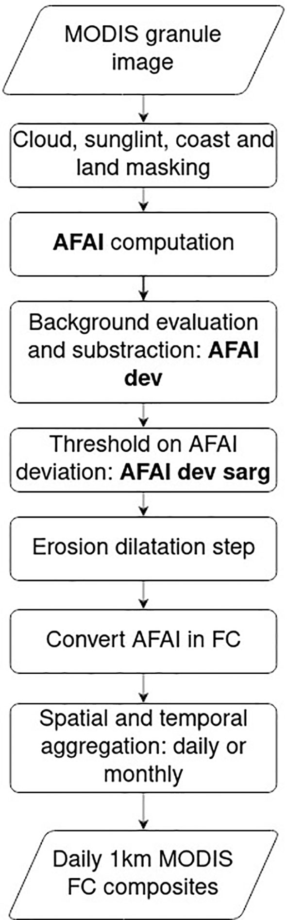
Figure 2 SAREDA work flow. Intermediate step of the data are indicated in bold.

That work flow was applied to the full archive of MODIS Level-1B (i.e. Top-of-the-atmosphere reflectance) granules (i.e., 5-minute orbit segments, 1354x2030 pixels 2300x2030 km² each) for both satellites. From those filtered AFAI images, the FC of the Sargassum algae was derived from AFAI with the ratio used by Wang and Hu (2016). FC values retrieved from Terra/MODIS and Aqua/MODIS were then mapped to an equirectangular grid and averaged daily and monthly. The mapped area extends from 15°S to 50°N and from 100°W to 15°E. The masked pixels were discarded in the average. We called those aggregated products composites. The daily composites provide a global view of Sargassum state in the North Atlantic. They are not exhaustive and contain gaps because of the cloud coverage and the gaps between MODIS swaths.

In this original dataset, Sargassum was distributed from the Gulf of Guinea to the Gulf of Mexico going through the Caribbean Sea. However, there was a high amount of suspicious detections. At high latitudes false detections were mainly caused by clouds and sun glint that were not completely removed from the data. In coastal areas, water turbidity can run over coastal mask in some cases and generate false detections (Wang and Hu, 2021). Finally, high chlorophyll concentration or other floating algae (such as Trichodesmium) are responsible for the remainder of false detections. These different phenomena cause a wide spatial distribution of false detections. Some of them are scattered in time and space, especially cloud resulting detections, while others are recurrent in some areas such as offshore chlorophyll production near the Mauritanian coasts. Finally, the fraction of false detections can exceed 50%. Examples of the different types of detection are presented in Figure 3.

FIGURE 3

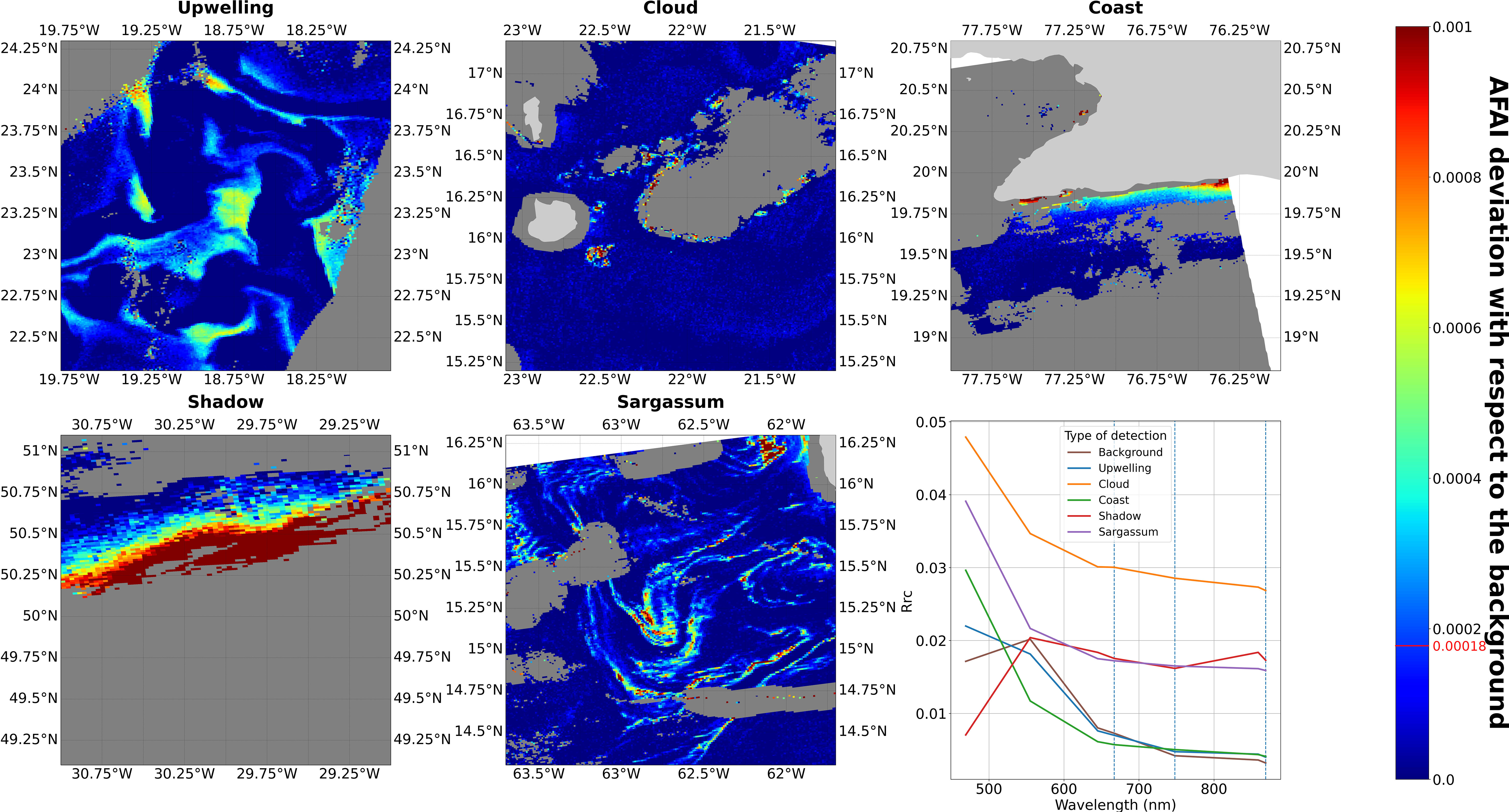
Figure 3 Examples of true and false detections for 2020 in 2° by 2° boxes. The colour bar indicates the AFAI deviation from the background (the AFAI detection threshold is indicated in red), masked pixels: either clouds, clouds shadows sunglint or shallow waters (<500 m depth) are represented in dark grey and land in light grey. The bottom right panel shows the average of Rayleigh-corrected reflectance spectra (Rrc) of each case and the background spectrum. Rrc was averaged over the detected pixels (not-detected pixel in the case of background) for each MODIS band in the range (400 nm - 800 nm). The bands used in the AFAI computation (667, 748, 869 nm) are shown as dashed blue lines.

2.3 Learning dataset, “expert truth”

In order to perform the filtering, it was necessary to establish a manually labelled dataset to train the model. A manual labelling was performed over FC daily composites by visual inspection (Wang and Hu, 2016; Cuevas et al., 2018; Qiu et al., 2018). We called that new dataset “expert truth” to differentiate it from real ground truth. To limit human validation bias, results obtained by three different operators were compared. All three labelled sets were consistent thus the operator bias was considered negligible.

The labelling process was based on daily vector images of the full North Atlantic area and set up with the graphical interface of QGIS (https://www.qgis.org). It was used for selecting and classifying the aggregations while displaying the AFAI images to analyse the surrounding context. Based on a daily 1 km Aqua-Terra composite and the corresponding full-resolution single-sensor non reprojected images (Level-2 products), we classified every aggregation except the ambiguous cases (< 5%).

The study focused on five years, 2016 to 2020, a period with continuous Sargassum presence. In order to ensure the model generalisation capability in spite of large seasonal and inter-annual variability of Sargassum algae, the learning dataset had to extent over a long time period to cover the different cases. The labelling process was divided evenly over the five years. Each year, we selected and validated 3 to 5 days spread out over the seasonal cycle. The dataset was thus representative of both an entire seasonal cycle and the five years of interest.

In the end, about 2000-2500 aggregations per year were labelled by the operators (Table 1), except for 2016 with less validated aggregations due to its lower Sargassum occurrence. Finally, there was about ten thousand labelled aggregations with 60% classified as true. While the true detections were more numerous than the false ones, their spatial extent was relatively smaller and they represented only 50% of the area.

TABLE 1

Table 1 Labelled aggregations per year.

2.4 Aggregations characterisation: spatial features extraction

The first kind of features used was the shape feature. At scales lower than 1 km, Sargassum algae aggregate in windrows (narrow elongated rafts) and patches (Ody et al., 2019), with extent between 1 and 100 m diameter. At scales greater than 1 km, the MODIS resolution only detects aggregations in the upper range of spatial extent, mostly typical large elongated structures. These filaments are a few kilometres wide and 10-100 kilometres long. Thus, a dozen shape indicators were extracted from the aggregations to characterise them (Jiao et al., 2012). Among those, an elongation index (Stojmenović and Žunić, 2008), a roundness index, a form complexity index, the area and the perimeter were extracted:

$\begin{array}{ll}Elongation=\frac{l_{\max }}{l_{\min }}& (1)\end{array}$

$\begin{array}{ll}Roundness=4*\frac{a}{\pi *l_{\max }^2}& (2)\end{array}$

$\begin{array}{ll}Formcomplexity=\frac{4\pi *a}{p^2}& (3)\end{array}$

Where l_max and l_min are the length of the major and minor axis of the aggregation, a and p its area and perimeter. Area and perimeter metrics take aggregations inner holes into account.

A second category of features was derived from the FC values within each aggregation. While the FC value of pixels considered independently does not allow false detection screening, as FC covers a wide range of valid values, the statistical distribution of these values within one aggregation can discriminate the false and the true Sargassum detections. Therefore, the mean, the median, the standard deviation, the minimum, the maximum and the interquartile range of the FC values within each aggregation were extracted.

The third kind of features was composed of several indices describing the surrounding of aggregations. As Sargassum aggregations are often small and close to each other, we defined the Nearest Neighbours Index (NNI) that counts the number of neighbouring aggregations within a given radius around one aggregation. Additionally, the Nearest Neighbours Area Index (NNAI) measures the total area covered by those close-by neighbours. Both of these indices were extracted with different radii from the barycentre of the aggregations.

In order to give more likelihood to redundant and time-coherent detections, an original persistence index (PersI) was developed. For every aggregation, it evaluates the number of times where the aggregation is close to at least one other aggregation in the two previous days and the two next days. Finally, the Coast Shortest Distance Index (CSDI) represents the aggregation distance from a land body.

In the end, around thirty indexed features were extracted. They were highly redundant, it was thus necessary to select the minimal subset of features to ensure the simplicity, the reliability and the robustness of the classification method. The feature selection was based on different sources of information. First, it took into account the correlation between indices to select uncorrelated features. Then, when it was available, it relied on the feature frequency of use during training with machine learning algorithms. Finally, the selection maximised the performance metrics of the algorithms (Section 2.5). Plus, the interpretability of the features was taken into account during the selection.

2.5 Classification algorithms selection and tuning

The last step of the method was to select the most suitable machine learning algorithm for the filtering and tune it. In order to evaluate and compare the performance of each algorithm, different scores were computed.

The classic performance scores used were the accuracy, the recall and the precision (Hastie et al., 2009), thereafter called “overall accuracy”, “overall recall” and “overall precision”. These scores were obtained with k-fold cross-validation on the whole dataset. In addition, we introduced the “generalisation accuracy”, the “generalisation recall” and the “generalisation precision” scores. First, the yearly accuracy, recall and precision were computed for each year using the remainder of the dataset as training dataset. The generalisation scores were defined as the average of those yearly scores. Those new metrics, needed because of the inter-annual variability of the Sargassum algae, represent the prediction capacity of the method over a completely unknown year. It thus gives a more realistic estimation of the method performance.

For selecting a machine learning algorithm, a benchmark was conducted over various classification algorithms. It included single model algorithms as Naive Bayes classifier (NB), Decision tree, Support Vector Machine (SVM), Linear Discriminant Analysis (LDA). Plus, some aggregated models based on decision trees were evaluated such as Adaboost, Gradient Tree Boosting (GTB), XGBoost and Random Forest (RF).

Several scores were computed to evaluate and compare the performance of each algorithm. First, the overall accuracy gives an overview of the algorithms performance. Yet, true Sargassum aggregations were more important in the classification to keep as much as possible the Sargassum signal. As overall accuracy weights evenly the classes, the overall recall was taken into account to focus on the true positive/false positive ratio. The overall precision was also computed but with lower attention for the optimisation as the false positive matter was less important. Finally, the overall f-score summarised these last two metrics but we mainly used the overall accuracy and the overall recall for interpretability.

Finally, those metrics were computed for all the tested algorithms using the python library scikit-learn (https://scikit-learn.org/) (Table 2). They were evaluated with a cross-validation step, by performing a k-fold over the labelled dataset (k = 50). The inputs were the 30 extracted aggregation features (Section 2.4). Usual algorithm performance ranking was retrieved, with aggregated methods with higher performances than single model methods. The single model methods, with low overall accuracy and overall recall (around 85% - 90%) but higher interpretability allowed to select the right features, especially the decision tree algorithm. Aggregated methods were very efficient with around 94% of overall accuracy but not easily interpretable. The random forest algorithm showed the best performance and was thus selected. This is consistent with the literature that repeatedly employs random forest for remote sensing classification (Belgiu and Drăguţ, 2016; Cuevas et al., 2018).

TABLE 2

Table 2 Algorithms performance computed with a k-fold operation (k = 50).

After selecting the random forest algorithm, a calibration was performed on its parameters to maximise the performance. Concerning the random forest algorithms calibration itself, the models were highly configurable. However, only two main parameters were evaluated here, the numbers of bootstrapped trees and the maximum depth of trees. Although random forests are not very sensitive to overfitting, the lowest values for tree depth (12) were taken to both conserve good performances and enhance generalisation power. Similarly, the number of estimators was chosen as small as possible (24) to reduce the computation time. We evaluated here both “overall accuracy” and “generalisation accuracy”. The set of input features was then reduced to a reasonable number in order to optimise performance (Section 2.4). For the NNI, the persistence index and the NNAI features, the radius maximising the scores for the NNI and NNAI computation was 700 km and the radius for the PersI computation was 50 km.

A learning curve was computed to check the convergence of the metrics. It was obtained by learning over an increasing fraction of the dataset, testing over the remainder, and computing both overall and generalisation scores. This was repeated 30 times to reduce random selection effect and then averaged in a single curve.

2.6 Time series production

The random forest classifier was applied to the daily FC composites over the time period 2016-2020 to build a filtered dataset. We obtained a complete filtered time series with one image of 1 km resolution per day.

Monthly composites were computed to overcome the extensive masking of daily products (mostly due to clouds), to enhance interpretability and for comparison with the literature (Wang and Hu, 2016; Ody et al., 2019). Finally, the FC was converted to wet biomass using the ratio of 3.34 proposed by Wang et al. (2018) based on field measurements in the Gulf of Mexico, the Florida Straits and Belize.

In order to summarise the whole time series (2016-2020), annual biomass averages were computed at 50 km resolution. A simplified envelope was also extracted for comparing spatial distributions between years. This envelope was obtained by first thresholding the 50 km composites (FC=10^-5). Then, the images were exported in vector format and erosion-dilation-erosion steps were applied to delete the remaining scattered aggregations and close gaps. Finally, for each pair of envelopes, the ratio between the intersected surface and the total surface was computed.

3 Results

The labelled dataset is shown in Figure 4, it gives an overview of the spatial distribution of true and false detections.

FIGURE 4

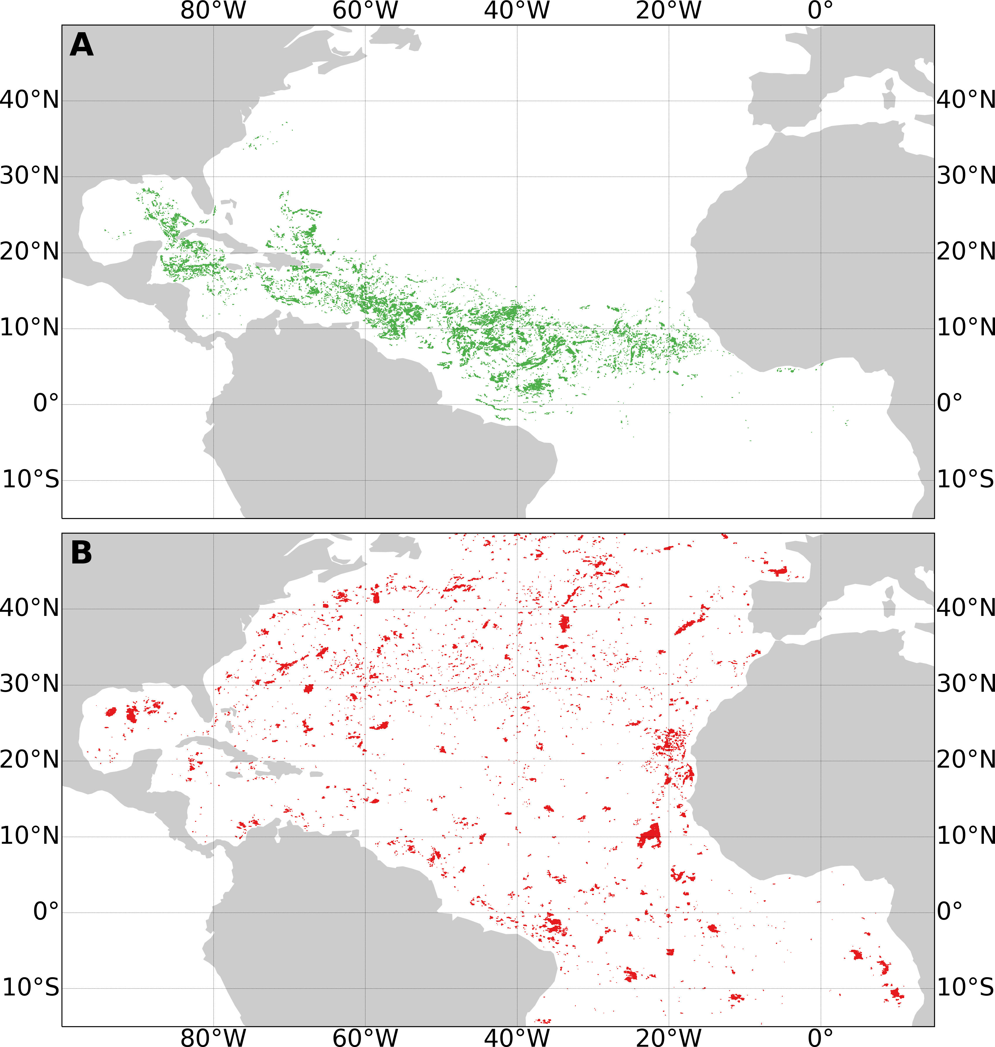
Figure 4 Map of true (A) and false (B) Sargassum aggregations from the learning dataset over 5 years. All labelled aggregations were displayed at their location, with possible overlaps.

True detections are concentrated from the Gulf of Guinea to the Gulf of Mexico, going through the central Atlantic and the Caribbean Sea. The false detection distribution was more spread out over the whole area with some dense areas like offshore Mauritania.

The whole set of features used in the classifier was reduced to five according to the performance maximisation of the filtering: NNI, CSDI, PersI, NNAI and the FC standard deviation (Table 3). Concerning the NNI, the PersI and the NNAI, they were selected regardless of the neighbourhood radius used and then calibrated.

TABLE 3

Table 3 Feature frequency of use (%) for the final classifier (random forest).

Table 3 shows the frequency of use for the five selected features. NNI is largely the most used while CSDI, PersI and NNAI are quite equivalent and the FC standard deviation is rarely used.

Concerning the classification performances, the learning curves computed on the dataset are presented in Figure 5. These learning curves show the fast convergence of the method performance. Both overall accuracy (recall and precision) and generalisation accuracy (recall and precision) stabilise when learning with more than half of the dataset. The generalisation accuracy (recall and precision) stabilises faster than the overall accuracy (recall and precision). The associated standard deviation was quite low thus the measurements were robust.

FIGURE 5

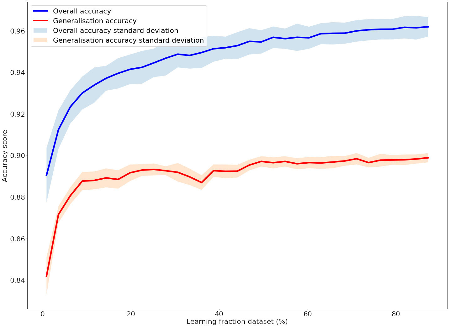
Figure 5 Learning curve of the random forest algorithm. The dataset fraction allocated for training increases from 3% to 90%, the remaining 10% of the data are used for testing. The displayed curves are the average on 30 computed curves. The blue curve shows the overall accuracy and the red curve the generalisation accuracy (i.e. training without a year and testing on it). Similar results were observed with the recall and precision scores.

In addition, the final scores of the method are shown in Table 4. The overall performance of our approach was about 96% regardless of the predicted class. The generalisation accuracy (recall and precision) per year varied between a minimum of 84% (83% and 82% respectively) in 2016 and between a maximum of 94% (96% and 96%) in 2019. The generalisation accuracy (recall and precision) is 90% on average (92% and 91%).

TABLE 4

Table 4 Algorithms performance scores in percentage.

Examples of composites before and after the filtering process at 1 and 50 km spatial resolutions are presented in Figure 6. A full seasonal cycle for the year 2020 at 50 km is shown in Figure 7.

FIGURE 6

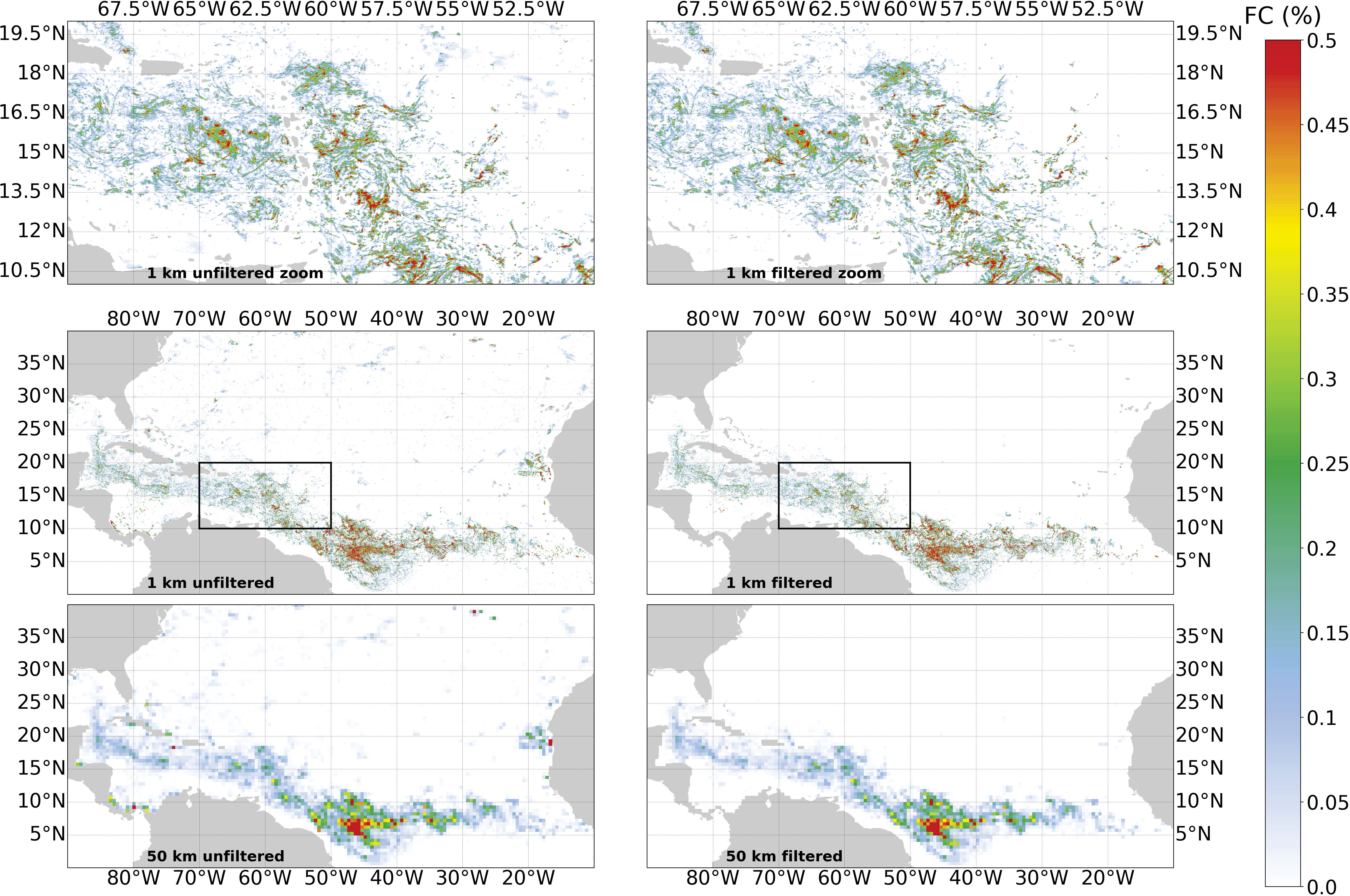
Figure 6 Monthly composite of FC for June 2020 at 1 km and 50 km resolution for unfiltered (left) and filtered (right) data. The top panel is a zoom of the region shown on middle panel.

FIGURE 7

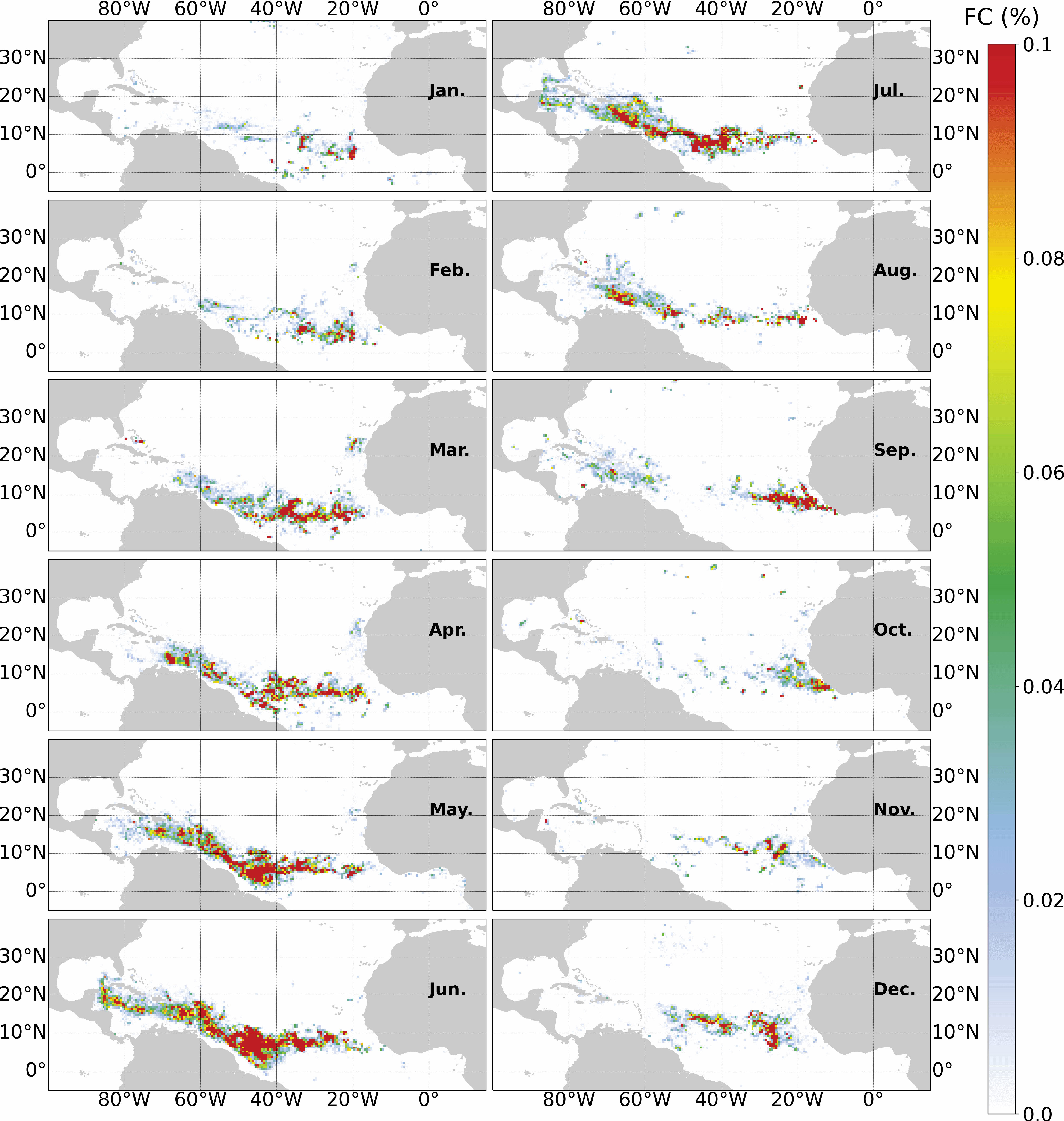
Figure 7 Filtered FC of monthly composites for 2020 at 50 km resolution.

The filtered products showed a coherent spatial distribution over the whole time series 2016-2020 (95% of accuracy is expected). False detections were removed in the areas where no Sargassum algae presence was reported (for example for latitudes > 30°N and< 0°N). In the opposite, the detected aggregations in the new Sargassum distribution area were retained (Figure 6).

The monthly time series of biomass in three different spatial boxes are displayed in Figure 8. The filtering method developed here reduced the biomass estimate by 40% in total for the whole time series and reduced the monthly estimate by 53% (average of monthly ratios). This is consistent with the estimated ratio of false detections observed in the learning dataset.

FIGURE 8

Figure 8 Sargassum biomass time series averaged in different boxes during the time period 2016-2020. The top panel displays the 2020 aggregated data in 1 km-resolution and the boxes used for the biomass computation. (A) presents the biomass time series in the same box as Wang et al. (2019) and compare it to their data (available until 2018 only). (B, C) are the retrieved Sargassum filtered biomass for Eastern and Western Atlantic Ocean (boxes B and C on the map). The black lines on the bar-plots indicate the annual mean of filtered data computed over the five years.

Primarily, over the North Tropical Atlantic, the seasonal cycle of biomass was rather regular (average of monthly standard deviation of 66%). The seasonal cycle of growth/decay leads to a biomass maximum in June and a minimum in November. The monthly average of biomass was estimated between 3 to 10 million tons. Biomass quantities were equivalent for 2017, 2019 and 2020 while 2016 and 2018 had respectively low and high biomass quantities. In addition to the global biomass time series, we computed separately the biomass from the Eastern and Western parts of the Tropical Atlantic Ocean to highlight their distinct dynamics. The Eastern area has lower Sargassum quantities with two biomass peaks in March and September. The Western area has 6 times greater biomass with only one peak in June. Concerning the boxes used for the biomass estimation in Figure 8, the limit of 30°W between the two areas was chosen both to maximise the differences between the two dynamics and to visually distinguish the two areas of high biomass.

For the years 2016-2018, unfiltered and filtered biomass estimates were compared to the Wang et al. (2019) time series. Our filtered biomass averaged over the three years was only 1% greater than Wang et al. (2019) estimate. Comparing month by month, there was a +4% difference on average, associated with a standard deviation of 33%. A student t-test was performed between the two datasets before and after filtering. Unfiltered data and Wang et al. (2019) data were significantly different with a p-value of 0.02 while filtered data was very similar to their measurements with a p-value of 0.97. Moreover, the filtered dataset was also close to their data in terms of spatial distribution (not shown). Besides, some remaining false detections and some true detections were absent in the results of Wang et al. (2019), while few of their detections were removed in the filtered dataset. The detailed analysis of these discrepancies could not be achieved here and was beyond the scope of this study. Finally, the main improvement of our dataset is the spatial resolution, 1 km for SAREDA filtered against 0.5° (≈50 km) for Wang et al. (2019) composites.

Lastly, the yearly Sargassum spatial distribution is presented in Figure 9 with simplified envelopes. By opposition to the high inter-annual biomass variations, the distribution areas do not differ much between years except in 2016. For example, the distribution area of 2018 is very similar to the area of 2017 despite the overall biomass being 3 times larger. In-depth comparison between annual distributions shows several areas of discrepancy: 1) the Gulf of Mexico, reached in 2018 and 2019 only; 2) The north of the Dominican Republic, overrun by Sargassum in 2017 and 2018 only; 3) The Central West Atlantic, where Sargassum algae usually remain above the equator except in 2019.

FIGURE 9

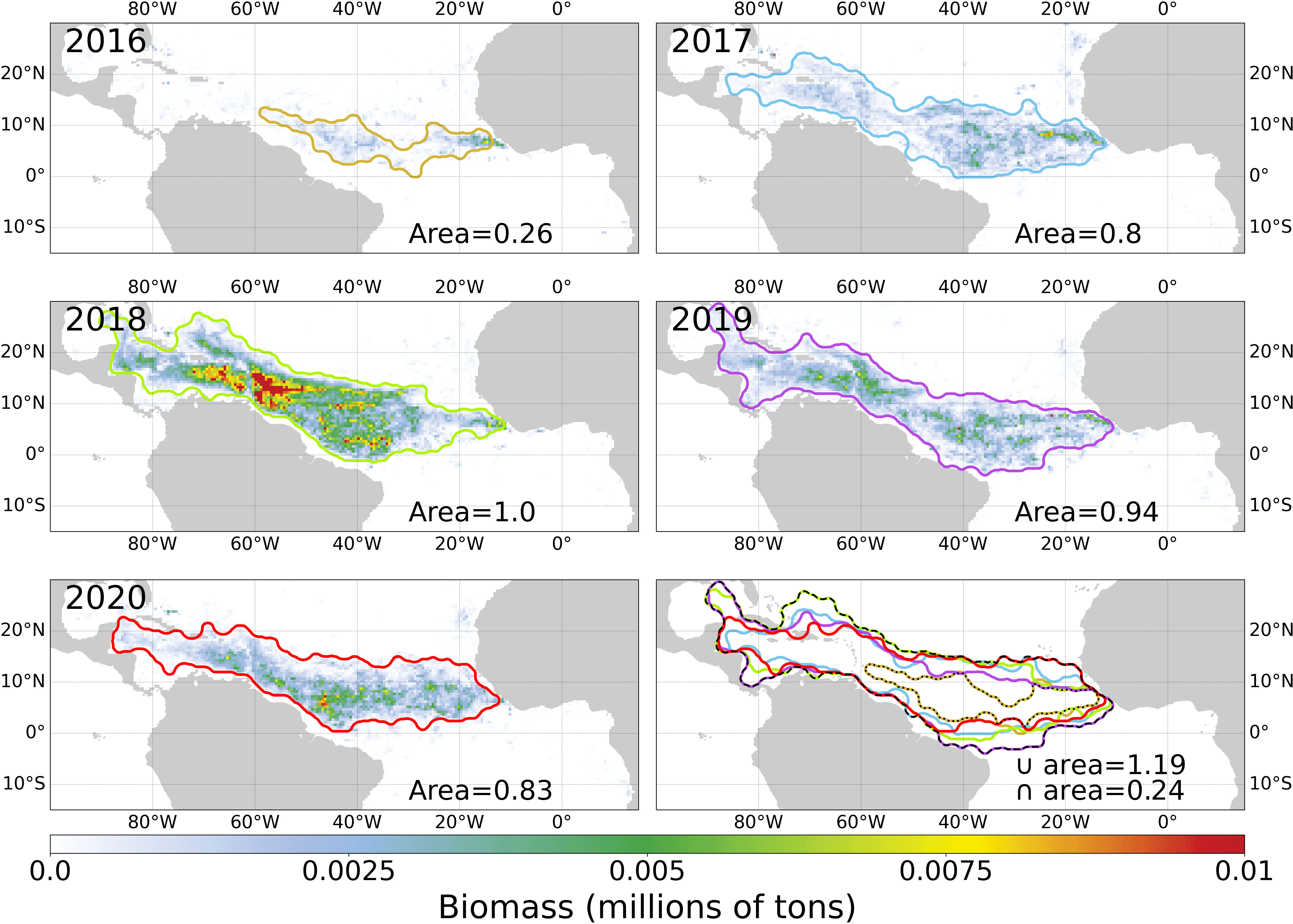
Figure 9 Annual composites of biomass at 50 km for 2016-2020 associated with the envelope of the area of high Sargassum concentration. The normalised envelope area with respect to 2018 (10.9 million of km²) is indicated. The last panel shows all the envelopes, its intersection (dotted line) and its union (dashed line).

4 Discussion

4.1 Interpretation of features used in the classification

Among the thirty features extracted from the detected aggregations, only five were used in the final classifier. The first selected feature and the most used in the classifier was the NNI (44.5%). This selection is consistent with visual observations during labelling, as true detections were mostly concentrated together in few areas. Besides, the major use of this feature was likely responsible for the lower classifier performance in 2016 where aggregations were scarce and sparse. The CSDI, the PersI and the NNAI completed the filtering by discriminating respectively the remaining coastal false detections and the far offshore Northern cloud false detections, the time-incoherent detections and the detections neighboured by large false detections due to chlorophyll concentration. Finally, the addition of the FC standard deviation increased the generalisation accuracy and the robustness of the method by preventing overfitting.

Only context indices were retained for the classification, likely because of the too coarse spatial resolution of the data. In particular, the elongation was not selected because of the fragmentation of aggregations. The elongated structures seen in the images were often split because of the erosion-dilatation operation used during the retrieval process (Section 2.2). We chose here to exclude location and temporal features from the selection. A test showed that including latitude and longitude coordinates greatly improved accuracy for a single year dataset but decreased accuracy with a more extended dataset. Furthermore, since the geographic distribution of the algae changed radically in 2010, we wanted to avoid geographical constraints.

4.2 Accuracy of the classification and generalisation

The performance scores obtained with the classifier were between 90% and 96%. The filtering quality for new data is expected to be in the annual generalisation scores range (90%). It will depend on the consistency of new data with the 2016-2020 dataset. The only lower-performing year was 2016 where the biomass level was much lower than other years. Overall, the score should stay around 90% if the current trend of biomass distribution persists. For the filtering of the 2011-2015 period, the performance obtained for 2016 should be representative and an accuracy above 85% is expected.

The learning curve analysis showed that increasing the learning set does not greatly improve scores. From 50% to 90% of the learning set, the overall score gained less than 1% of accuracy while the generalisation score was stable. Adding data from the same years 2016-2020 to the learning set will therefore be useless. The only way to noticeably improve the method would be to add data from other years and make both scores converge.

The performance is analogous to or better than other works that used machine learning algorithms for Sargassum detection. Cuevas et al. (2018) applied a random forest algorithm over a small dataset using raw reflectances and derived indices such as AFAI. Their accuracy was close to our study with an overall score of 93.4%. Arellano-Verdejo et al. (2019) used deep learning on radiometric inputs from MODIS to detect Sargassum. Their accuracy was similar to our results (90%). Finally, studies on Yellow Sea Sargassum algae (Qiu et al., 2018; Shin et al., 2021) showed similar or lower performance.

4.3 Limits of the method and potential improvements

The choice of MODIS imagery implies rather coarse resolution but recurring observations (twice a day). We used the 1 km bands for AFAI computation to ensure good signal/noise ratio compared to 250 - 500 m bands and to better discriminate between Sargassum and clouds (Wang and Hu, 2016). Comparison of AFAI with high resolution (20 m) MSI observations have shown that both estimates are consistent (Wang and Hu, 2020; Descloitres et al., 2021). MODIS appears as a trade-off between regular mapping of the Sargassum distribution and resolution.

The method assumed that features distribution is consistent for all aggregations regardless of their location and of their time of observation. This is mostly the case over the studied time period, as the high performance obtained by the method demonstrates a good spatial and temporal consistency. Yet, specific regions or periods may show singular distributions of features. That could be the case for areas where false detections remained after the filtering process, such as offshore Mauritania or the Amazon plume area. The global approach could be limited here and defining regional learning sets and classifiers may improve the method performance.

The learning set was built to be as representative as possible of the whole set of true and false detections. Nonetheless, in some areas (e.g., Gulf of Guinea, Sargasso Sea), discrimination between true and false detections was more strenuous for manual labelling. Both low Sargassum concentration and cloud coverage created ambiguous cases. This induced a lack of labelled data and most likely a lower filtering accuracy in these regions. Remote sensing imagery from other sensors with higher resolution or in-situ measurements could help to fill this gap and to ensure the completeness of the dataset.

Since the study focused on basin scale offshore Sargassum detection, coastal areas were masked. This choice does not have a large impact on Sargassum estimation as detections in the coastal areas were mostly false detections. Tests using our classification algorithm to filter out coastal false detections and avoid masking coastal waters were not conclusive. In coastal areas, progress in Sargassum detection can be made using other sensors/indices with poorer temporal resolution, such as OLCI and Maximum Chlorophyll Index (Gower and King, 2011), less sensitive to coastal contamination, or higher resolution sensors such as MSI (Wang and Hu, 2020, 2021). Those sensors would be useful to complement MODIS data.

4.4 Uncertainties in the Sargassum estimates

Sargassum detection is limited by algae observability. In certain circumstances (low density, vertical mixing in the upper layer), MODIS cannot distinguish Sargassum from background (Woodcock, 1950; Johnson and Richardson, 1977; Woodcock, 1993; Wang and Hu, 2020). This limitation is outside the scope of our study.

Concerning the filtered products, clues on their uncertainties were given by the classifier performance study. For the 2016-2020 period, the expected errors fraction would be about 2.5% of false positives and 2.5% false negatives. As the false aggregations are larger than true ones, false positives would induce a greater overestimation than false negatives generate an underestimation. Thus, the filtering errors are expected to produce a small overestimation with errors on some Sargassum aggregations locations. For data from other years, the reasoning is the same but with around 5% of false positives and of false negatives generating an overestimation twice larger.

Concerning the aggregated products, there is an uncertainty due to the sampling, limited by the coverage of daily data. With two observations per day over the whole Tropical Ocean, only 30% of pixels were retrieved because of the different masks. The solution used to fill these gaps was to aggregate data spatially or temporally. In order to keep the best spatial resolution, temporal averaging was used. If we hypothesise a fully random mask distribution (binomial distribution for every pixel), 6 days are needed to reach a coverage of at least 90%. In practice, 12 days were needed. The temporal composites based on less than 12 days were therefore incomplete while using more than 12 days reduce mapping accuracy because of non negligible Sargassum drift.

4.5 Sargassum dynamics over 2016-2020

The biomass fluctuations resulted mainly from advection for 1-2 month timescale (Berline et al., 2020), while biology (growth and decay) combined to advection drives the fluctuations for longer time scales. Our results strengthened the scenario of recirculation of the Sargassum biomass in the North Tropical Atlantic: from the development of relatively low biomass in the Eastern Atlantic Ocean in the early months of the year, advection inseminates the Central Atlantic Ocean and leads to a biomass maximum in June-July. In addition to the bloom transport in the Caribbean Sea and the Gulf of Mexico, some Sargassum algae are driven back eastwards by the North Equatorial Countercurrent (NECC) causing the September peak of biomass. Finally, the algae globally decay and return to a global minimum of biomass in November. This cycle, rather stable over the studied period (2016-2020), is consistent with the time series from Wang et al. (2019) over 2016-2018.

The eastern and western boxes essentially distinguish the western and eastern consolidation regions from Franks et al. (2016). This limit also matches the transition between two distinct areas of annual biomass production, as shown on the 2020 seasonal biomass cycle (see top of Figure 8). The two different dynamics and biomass quantities observed in the Eastern and Western Tropical Atlantic Ocean are consistent with the simulations from Jouanno et al. (2021a) (their Figure 5) for the year 2017.

As a perspective, the 1 km resolution of our dataset may allow tracking algae aggregations over several days of observations. This tracking could provide valuable inputs on Sargassum drift patterns. Such an approach was recently tested with GOES (Geostationary Operational Environmental Satellite) by Minghelli et al. (2021) with 15-minute observations, but with a lower sensitivity. To validate the analysis of the Sargassum distribution dynamics and explore the anomalous 2010 event (Johns et al., 2020), the filtered dataset will be extended backwards to 2000, i.e. over the full MODIS archive (only Terra sensor for 2000-2001).

5 Conclusion

With the use of a machine learning algorithm, this study benefits from an untapped source of information: the spatial context of Sargassum aggregations. Those new features are complementary with radiometric data used in previous approaches and allow to screen false detections induced by various phenomena. While classic algorithms have known flaws that induce false detections, the post-processing filtering technique presented here offers a solution to identify and mitigate those flaws and produce automatically a high-quality product over a large-scale area. As the method is time and space independent and modular, it would be easily generalised to other Sargassum detection datasets or other application scopes. The Sargassum annual cycle of the filtered dataset is consistent with the literature for seasonal and inter-annual fluctuations and we provided a detailed characterisation of the spatial variability of the distribution. As a perspective, the filtering process will be implemented in the SAREDA pipeline to provide near real-time filtered products and reprocess the past time series. This dataset will be useful to understand the drivers of Sargassum dynamics at fine and large scale and validate future models.

Data availability statement

The raw data supporting the conclusions of this article will be made available by the authors, without undue reservation.

Author contributions

WP developed the core of the filtering method. JD processed the remote sensing data from MODIS. CC, AM and CL have participated the methodology building. LB led the project. All authors contributed to the article and approved the submitted version.

Funding

The Ph.D. ofWitold Podlejski is funded by ANR FORESEA (FORESEA project, grant ANR-19-SARG-0007).

Acknowledgments

Authors thank TOSCA-CNES and IRD for funding the project SAREDA-DA allowing the production of the MODIS Sargassum detection dataset. GeoID-Ocean is thanked for the early prototyping of the processing chain. AERIS-ICARE is thanked for providing processing infrastructure for the production of the dataset.

Conflict of interest

The authors declare that the research was conducted in the absence of any commercial or financial relationships that could be construed as a potential conflict of interest.

Publisher’s note

All claims expressed in this article are solely those of the authors and do not necessarily represent those of their affiliated organizations, or those of the publisher, the editors and the reviewers. Any product that may be evaluated in this article, or claim that may be made by its manufacturer, is not guaranteed or endorsed by the publisher.

References

Arellano-Verdejo J., Lazcano-Hernandez H. E., Cabanillas-Terán N. (2019). Erisnet: deep neural network for sargassum detection along the coastline of the mexican caribbean. PeerJ 7, e6842. doi: 10.7717/peerj.6842

PubMed Abstract | CrossRef Full Text | Google Scholar

Belgiu M., Drăguţ L. (2016). Random forest in remote sensing: A review of applications and future directions. ISPRS J. photogramm. Remote Sens. 114, 24–31. doi: 10.1016/j.isprsjprs.2016.01.011

CrossRef Full Text | Google Scholar

Berline L., Ody A., Jouanno J., Chevalier C., André J.-M., Thibaut T., et al. (2020). Hindcasting the 2017 dispersal of sargassum algae in the tropical north atlantic. Mar. pollut. Bull. 158, 111431. doi: 10.1016/j.marpolbul.2020.111431

PubMed Abstract | CrossRef Full Text | Google Scholar

Chávez V., Uribe-Martínez A., Cuevas E., Rodríguez-Martínez R. E., van Tussenbroek B. I., Francisco V., et al. (2020). Massive influx of pelagic sargassum spp. on the coasts of the mexican caribbean 2014–2020: challenges and opportunities. Water 12, 2908. doi: 10.3390/w12102908

CrossRef Full Text | Google Scholar

Chen Y., Wan J., Zhang J., Zhao J., Ye F., Wang Z., et al. (2019) in IGARSS 2019-2019 IEEE International Geoscience and Remote Sensing Symposium (IEEE). 3705–3707. doi: 10.1109/IGARSS.2019.8898131

CrossRef Full Text | Google Scholar

Cuevas E., Uribe-Martínez A., Liceaga-Correa M.d. l. Á. (2018). A satellite remote-sensing multi-index approach to discriminate pelagic sargassum in the waters of the yucatan peninsula, mexico. Int. J. Remote Sens. 39, 3608–3627. doi: 10.1080/01431161.2018.1447162

CrossRef Full Text | Google Scholar

Descloitres J., Minghelli A., Steinmetz F., Chevalier C., Chami M., Berline L. (2021). Revisited estimation of moderate resolution sargassum fractional coverage using decametric satellite data (s2-msi). Remote Sens. 13, 5106. doi: 10.3390/rs13245106

CrossRef Full Text | Google Scholar

Dierssen H., Chlus A., Russell B. (2015). Hyperspectral discrimination of floating mats of seagrass wrack and the macroalgae sargassum in coastal waters of greater florida bay using airborne remote sensing. Remote Sens. Environ. 167, 247–258. doi: 10.1016/j.rse.2015.01.027

CrossRef Full Text | Google Scholar

Fine M. L. (1970). Faunal variation on pelagic sargassum. Mar. Biol. 7, 112–122. doi: 10.1007/BF00354914

CrossRef Full Text | Google Scholar

Franks J. S., Johnson D. R., Ko D. S. (2016). Pelagic sargassum in the tropical north atlantic. Gulf Caribbean Res. 27, SC6–SC11. doi: 10.18785/gcr.2701.08

CrossRef Full Text | Google Scholar

Gower J., Hu C., Borstad G., King S. (2006). “Ocean color satellites show extensive lines of floating sargassum in the gulf of mexico,” in IEEE Transactions on Geoscience and Remote Sensing, Vol. 44. 3619–3625. doi: 10.1109/TGRS.2006.882258

CrossRef Full Text | Google Scholar

Gower J. F., King S. A. (2011). Distribution of floating sargassum in the gulf of mexico and the atlantic ocean mapped using meris. Int. J. Remote Sens. 32, 1917–1929. doi: 10.1080/01431161003639660

CrossRef Full Text | Google Scholar

Gower J., King S. (2020). The distribution of pelagic sargassum observed with olci. Int. J. Remote Sens. 41, 5669–5679. doi: 10.1080/01431161.2019.1658240

CrossRef Full Text | Google Scholar

Hastie T., Tibshirani R., Friedman J. (2009). The elements of statistical learning: data mining, inference, and prediction (Springer Science & Business Media). New York: Springer.

Google Scholar

Hu C., Feng L., Hardy R. F., Hochberg E. J. (2015). Spectral and spatial requirements of remote measurements of pelagic sargassum macroalgae. Remote Sens. Environ. 167, 229–246. doi: 10.1016/j.rse.2015.05.022

CrossRef Full Text | Google Scholar

Jiao L., Liu Y., Li H. (2012). Characterizing land-use classes in remote sensing imagery by shape metrics. ISPRS J. Photogramm. Remote Sens. 72, 46–55. doi: 10.1016/j.isprsjprs.2012.05.012

CrossRef Full Text | Google Scholar

Johns E. M., Lumpkin R., Putman N. F., Smith R. H., Muller-Karger F. E., Rueda-Roa D. T., et al. (2020). The establishment of a pelagic sargassum population in the tropical atlantic: biological consequences of a basin-scale long distance dispersal event. Prog. Oceanogr. 182, 102269. doi: 10.1016/j.pocean.2020.102269

CrossRef Full Text | Google Scholar

Johnson D. L., Richardson P. L. (1977). On the wind-induced sinking of sargassum. J. Exp. Mar. Biol. Ecol. 28, 255–267. doi: 10.1016/0022-0981(77)90095-8

CrossRef Full Text | Google Scholar

Jouanno J., Benshila R., Berline L., Soulié A., Radenac M.-H., Morvan G., et al. (2021a). A nemo-based model of sargassum distribution in the tropical atlantic: description of the model and sensitivity analysis (nemo-sarg1. 0). Geosci. Model. Dev. 14, 4069–4086. doi: 10.5194/gmd-14-4069-2021

CrossRef Full Text | Google Scholar

Jouanno J., Moquet J.-S., Berline L., Radenac M.-H., Santini W., Changeux T., et al. (2021b). Evolution of the riverine nutrient export to the tropical atlantic over the last 15 years: is there a link with sargassum proliferation? Environ. Res. Lett. 16, 034042. doi: 10.1088/1748-9326/abe11a

CrossRef Full Text | Google Scholar

Martin L. M., Taylor M., Huston G., Goodwin D. S., Schell J. M., Siuda A. N. (2021). Pelagic sargassum morphotypes support different rafting motile epifauna communities. Mar. Biol. 168, 1–17. doi: 10.1007/s00227-021-03910-2

CrossRef Full Text | Google Scholar

Merle H., Resière D., Mesnard C., Pierre M., Jean-Charles A., Béral L., et al. (2021). Case report: Two cases of keratoconjunctivitis tied to sargassum algae emanations. Am. J. Trop. Med. Hyg. 104, 403–405. doi: 10.4269/ajtmh.20-0636

PubMed Abstract | CrossRef Full Text | Google Scholar

Minghelli A., Chevalier C., Descloitres J., Berline L., Blanc P., Chami M. (2021). Synergy between low earth orbit (leo)–modis and geostationary earth orbit (geo)–goes sensors for sargassum monitoring in the atlantic ocean. Remote Sens. 13, 1444. doi: 10.3390/rs13081444

CrossRef Full Text | Google Scholar

Ody A., Thibaut T., Berline L., Changeux T., André J.-M., Chevalier C., et al. (2019). From in situ to satellite observations of pelagic sargassum distribution and aggregation in the tropical north atlantic ocean. PloS One 14, e0222584. doi: 10.1371/journal.pone.0222584

PubMed Abstract | CrossRef Full Text | Google Scholar

Oviatt C. A., Huizenga K., Rogers C. S., Miller W. J. (2019). What nutrient sources support anomalous growth and the recent sargassum mass stranding on caribbean beaches? a review. Mar. pollut. Bull. 145, 517–525. doi: 10.1016/j.marpolbul.2019.06.049

PubMed Abstract | CrossRef Full Text | Google Scholar

Qiu Z., Li Z., Bilal M., Wang S., Sun D., Chen Y. (2018). Automatic method to monitor floating macroalgae blooms based on multilayer perceptron: case study of yellow sea using goci images. Optics express 26, 26810–26829. doi: 10.1364/OE.26.026810

PubMed Abstract | CrossRef Full Text | Google Scholar

Resiere D., Valentino R., Nevière R., Banydeen R., Gueye P., Florentin J., et al. (2018). Sargassum seaweed on caribbean islands: an international public health concern. Lancet 392, 2691. doi: 10.1016/S0140-6736(18)32777-6

CrossRef Full Text | Google Scholar

Shin J., Lee J.-S., Jang L.-H., Lim J., Khim B.-K., Jo Y.-H. (2021). Sargassum detection using machine learning models: A case study with the first 6 months of goci-ii imagery. Remote Sens. 13, 4844. doi: 10.3390/rs13234844

CrossRef Full Text | Google Scholar

Stojmenović M., Žunić J. (2008). Measuring elongation from shape boundary. J. Math. Imaging Vision 30, 73–85. doi: 10.1007/s10851-007-0039-0

CrossRef Full Text | Google Scholar

Wang M., Hu C. (2016). Mapping and quantifying sargassum distribution and coverage in the central west atlantic using modis observations. Remote Sens. Environ. 183, 350–367. doi: 10.1016/j.rse.2016.04.019

CrossRef Full Text | Google Scholar

Wang M., Hu C. (2018). On the continuity of quantifying floating algae of the central west atlantic between modis and viirs. Int. J. Remote Sens. 39, 3852–3869. doi: 10.1080/01431161.2018.1447161

CrossRef Full Text | Google Scholar

Wang M., Hu C. (2020). “Automatic extraction of sargassum features from sentinel-2 msi images,” in IEEE Transactions on Geoscience and Remote Sensing. 1–19. doi: 10.1109/TGRS.2020.3002929

CrossRef Full Text | Google Scholar

Wang M., Hu C. (2021). Satellite remote sensing of pelagic sargassum macroalgae: The power of high resolution and deep learning. Remote Sens. Environ. 264, 112631. doi: 10.1016/j.rse.2021.112631

CrossRef Full Text | Google Scholar

Wang M., Hu C., Barnes B. B., Mitchum G., Lapointe B., Montoya J. P. (2019). The great atlantic sargassum belt. Science 365, 83–87. doi: 10.1126/science.aaw7912

PubMed Abstract | CrossRef Full Text | Google Scholar

Wang M., Hu C., Cannizzaro J., English D., Han X., Naar D., et al. (2018). Remote sensing of sargassum biomass, nutrients, and pigments. Geophys. Res. Lett. 45, 12–359. doi: 10.1029/2018GL078858

CrossRef Full Text | Google Scholar

Woodcock A. H. (1950). Subsurface pelagic sargassum. J. Mar. Res. 9, 77–92. Available at: link: https://images.peabody.

Google Scholar

Woodcock A. H. (1993). Winds subsurface pelagic sargassum and langmuir circulations. J. Exp. Mar. Biol. Ecol. 170, 117–125. doi: 10.1016/0022-0981(93)90132-8

CrossRef Full Text | Google Scholar

Xing Q., Guo R., Wu L., An D., Cong M., Qin S., et al. (2017). “High-resolution satellite observations of a new hazard of golden tides caused by floating sargassum in winter in the yellow sea,” in IEEE Geoscience and Remote Sensing Letters, Vol. 14. 1815–1819. doi: 10.1109/LGRS.2017.2737079

CrossRef Full Text | Google Scholar