Abstract
Submesoscale processes in the ocean vary rapidly in both space and time, and are often difficult to capture by field observations. Their dynamical connection with marine biology remains largely unknown because of the intrinsic link between temporal and spatial variations. In May 2015, satellite chlorophyll data demonstrated high concentration patches in the edge region between mesoscale eddies, which were higher than those in the cyclonic eddy core region in the northern South China Sea (NSCS). The underlying mechanisms were examined with a high-resolution physical-biological model. By tracking Lagrangian particles in the model, this study shows that the edge region between eddies is a submesoscale frontal region that is prone to intense upwelling and downwelling motions. We identified two key submesoscale mechanisms that affect nutrient transport flux significantly, submesoscale fontal dynamics and submesoscale coherent eddies. The dynamics associated with these two mechanisms were shown to be able to inject subsurface nutrients into the upper layer, generate the high chlorophyll patch, and alter phytoplankton community structure in the NSCS. This study shows the importance of submesoscale processes on phytoplankton dynamics in the NSCS and highlights the need for high-resolution observations.
Introduction
Mesoscale eddies are a ubiquitous feature and important in regulating physical and biogeochemical environments in the ocean (e.g., Falkowski et al., 1991; McGillicuddy et al., 1998; McGillicuddy et al., 2007; Chelton et al., 2011; Siegel et al., 2011; Mahadevan et al., 2012; Gaube et al., 2013; Omand et al., 2015). Regions around mesoscale eddies are known to be associated with strong current shear and strain, which can induce intense upward and downward motions at submesoscale (Lapeyre et al., 2006; Mahadevan and Tandon, 2006). These vertical motions can efficiently transport nutrients into the euphotic zone and lead to elevated biological patches (Lévy et al., 2001; Lehahn et al., 2007; Mahadevan, 2016).
In the ocean, vertical velocities are generally orders of magnitude smaller than horizontal ones (Klein and Lapeyre, 2009), and direct measurements of vertical velocities are not currently available. With the Omega equation, one can diagnose the vertical velocity by using measured density and velocity fields (e.g., Martin and Richards, 2001). Legal et al. (2007) reported an anticorrelation between vertical velocity and density gradient in a frontal region, and suggested that the large-scale strain can dynamically change small-scale filaments. The edge region of a mesoscale eddy or between eddies can be treated as a front because of the horizontal density gradient. Klein and Lapeyre (2009) thus suggested that the vertical exchange should be more efficient at the eddy edge than eddy center.
In addition to fronts, submesoscale eddies that are defined as energetic eddies with a radius smaller than the Rossby deformation radius and a localized structure, have also been observed in different parts of the ocean (McWilliams, 1985; Li et al., 2017; Zhang et al., 2022). They can be very long lived and travel far from their origins. As they can retain their core water mass during their life, they can transport waters with anomalous properties over long distances (Lukas and Santiago-Mandujano, 2001). The cumulative effect of these submesoscale eddies can potentially affect the large-scale transport and distribution of heat, nutrients, and other materials (e.g., Frenger et al., 2018; Gula et al., 2019).
The South China Sea (SCS) is an oligotrophic marginal sea adjacent to the western Pacific Ocean. Seasonally changing monsoon winds play an important role in modulating the upper ocean biology (Liu et al., 2002; Gan et al., 2006). Superimposed on the basin-scale variability, significant spatial and temporal variations of phytoplankton dynamics have been found to be related to mesoscale eddies (Ning et al., 2004; Chen et al., 2007; Huang et al., 2010; Xiu and Chai, 2011; Guo et al., 2015; He et al., 2016; Liu et al., 2017; Xiu et al., 2019). Most of the eddies show high chlorophyll concentrations in the cyclonic eddy core and low concentrations in the anticyclonic eddy core, which is likely related to the mesoscale eddy mechanism (McGillicuddy et al., 1998). A lot of studies have been conducted focusing on physical characteristics of submesoscale features in the northern SCS (Liu et al., 2010; Zhang et al., 2016; Dong and Zhong, 2018; Qiu et al., 2019; Ni et al., 2021; Zhang et al., 2022). However, less attention has been given to the biological impact from submesoscale processes at the eddy edge where enhanced shear and strain exist. Observations from Zhou et al. (2013) and Wang et al. (2018) indicated that possible submesoscale structures around an anticyclonic eddy may enhance phytoplankton production and increase carbon export; however, their samplings were too coarse in space (30-50 km) to resolve detailed submesoscale dynamics. With satellite data in the western SCS, Liu et al. (2017) showed high chlorophyll anomaly present at the northwestern periphery of anticyclonic eddies and suggested that it could be induced by the ageostrophic secondary circulation.
The submesoscale process has a typical spatial scale of 1-10 km and a temporal scale of ~1 day that are difficult to observe by coarse-resolution ship measurements or regular-frequency Argo floats. How these submesoscale processes affect phytoplankton and nutrient distributions in the northern SCS (NSCS), however, remains largely unknown. Moreover, the high energy of the submesoscale field also has significant implications for predictive modeling of oceanic pollutant pathways and concentrations. In this study, a high-resolution physical-biological model was built to investigate the influence of submesoscale features around mesoscale eddies on biological processes in the NSCS.
Data and model
To study biological responses to submesoscale structures, a coupled physical-biological model was developed for the NSCS region. The physical model was based on the Regional Ocean Modelling System (ROMS), and the biological model was based on a modified version of the Carbon Silicate Nitrate Ecosystem (CoSiNE; Chai et al., 2002) model. This modified version of CoSiNE model includes two phytoplankton groups (small phytoplankton with S1 for nitrogen based biomass and Chl1 for chlorophyll concentration, diatom with S2 for nitrogen based biomass, and Chl2 for chlorophyll concentration), two zooplankton classes (microzooplankton (Z1), mesozooplankton (Z2)), two size classes of detritus (small (SPON), large (LPON)), biogenic silica (bSi), nitrate (NO3), ammonium (NH4), silicate (SiOH4), phosphate (PO4), dissolved inorganic carbon (DIC), total alkalinity (TALK) and dissolved oxygen (DO). In the model, both small phytoplankton and diatom uptake the NO3, NH4, and PO4 for growth, and diatom needs extra nutrient, SiOH4. The microzooplankton grazes on small phytoplankton, while the mesozooplankton grazes on diatoms, microplankton, and detritus. The mortality and aggregation of phytoplankton and zooplankton are the source terms of detritus. Predation by mesozooplankton and the remineralization are the sink terms of detritus. The detailed model equations and parameters can be found in Ma et al. (2019).
The three-dimensional coupled model was set up for the NSCS (116-120° E, 18-22°N). It has a 1/108° (~ 1 km) resolution horizontally and has 30 vertical levels in terrain-following sigma-coordinates. The coupled model was initialized and one-way nested to the Hybrid Coordinate Ocean Model (HYCOM) dataset that has a spatial resolution of 1/12° and a temporal resolution of 1 day. The HYCOM model uses the Navy Coupled Ocean Data Assimilation system (NCODA) to assimilate available altimeter data, satellite, in-situ profiles from XBTs, buoys and Argo floats, which gives a better representation of the state of the ocean. In addition, eight tidal constituents (M2, S2, N2, K2, K1, O1, P1, and Q1) were used to calculate the hourly tidal elevation at the boundary. Here, M2 is the principal lunar semidiurnal constituent, S2 is the principal solar semidiurnal constituent, N2 is the larger lunar elliptic semidiurnal constituent, K2 is the luni-solar semidiurnal constituent, K1 is the luni-solar diurnal constituent, O1 is the principal lunar diurnal constituent, P1 is the principal solar diurnal constituent, and Q1 is the larger lunar elliptic constituent. For the surface forcing, the 6-hourly surface winds were obtained from the Cross-Calibrated Multi-Platform (CCMP) wind dataset with a spatial resolution of 0.25°. The surface heat and freshwater fluxes were calculated by the COARE3.0 bulk formula using both the CCMP wind and 6-hourly NCEP/NCAR reanalysis data. The initial and boundary conditions for biological variables were derived from a coarse-resolution coupled model, which covers the Pacific Ocean and runs continuously from 1993 to present (Xiu and Chai, 2011).
The coupled model was integrated from 1 January 2015 for one year and daily averaged model outputs were used for analysis. Model outputs were further used to drive an offline particle tracking code (TRACMASS; https://www.tracmass.org/) to examine vertical motions. The TRACMASS code was developed by Döös (1995), which computes numerically the trajectory through each grid cell by solving a differential equation that depends on the velocities on the grid box wall. The chosen water trajectories from any location can be followed along the path both forward and backward in time.
Daily sea-level anomaly (SLA) field with a grid of 1/4° by 1/4° was obtained from the Archiving, Validation and Interpretation of Satellite Data in Oceanography (AVISO). The finite-size Lyapunov exponent (FSLE) product was also obtained from AVISO, which is commonly used to diagnose regions of large stretching and straining by advection (d’Ovidio et al., 2004). The FSLE is defined as the inverse time of separation of two particles from their initial distance to final distance. The particles were advected by altimetry velocities and their trajectories are computed by backward-time integrating the altimetry velocities. Thus, regions with large FSLE generally correspond to the regions where surface current divergence are strong. Chlorophyll concentration data was obtained from a multi-sensor (SeaWiFS, MODIS and MERIS) merged product with a spatial resolution of 4 km and a temporal resolution of 1 day, developed by the Ocean Color Climate Change Initiative (OC_CCI) (Lavender et al., 2015). For analysis, the SLA and FSLE were interpolated onto the chlorophyll data grid.
Results
Submesoscale features between eddies
On 28 April 2015, two cyclonic eddies were present to the west of Luzon Strait, with one located on the north (CE1) and the other one on the south (CE2). There was another anticyclonic eddy (AC1) present to the west of the two cyclonic eddies (Figure 1). The water property in AC1 was similar to that of Kuroshio water, suggesting that the AC1 was generated by Kuroshio intrusion (Shu et al., 2016). When tracing back to February 2015, we can see that the two CEs were generated locally in the NSCS (Shu et al., 2016). The locations of the three eddies were relatively stable between late April and early May. The strength of the two CEs gradually reduced after early May, while the AC maintained its strength and propagated to the west.
Figure 1
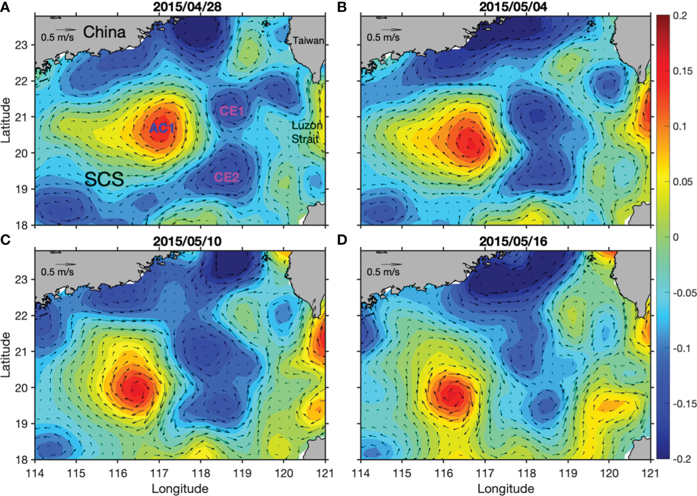
Time evolutions of SLA (units: m) overlaid by geostrophic current anomalies on 28 April (A), 04 May (B), 10 May (C) and 16 May 2015 (D).
Satellite-derived surface chlorophyll concentration showed clearly localized high patches with magnitude higher than 0.15 mg m-3 in the edge regions between CE1 and CE2, and between AC1 and the CEs (Figures 2A, B). Due to cloud contamination, we can only show four-day-averaged chlorophyll concentration, which is not fine enough to resolve detailed submesoscale dynamics. For the daily chlorophyll data, the mean cloud coverage in the study region in April and May was about 76% and it reduced to about 31% when using the four-day-averaged data. Unlike physical variables, it usually takes days for phytoplankton to show biological changes in response to dynamical forcings. Four-day-averaged chlorophyll is probably able to reflect biological changes to submesoscale dynamics, but locations might not be consistent with physical variables (Mahadevan, 2016; Lévy et al., 2018). The spatial decoupling between upwelling, phytoplankton new production, and export production across a submesoscale front has been reported (Estapa et al., 2015). Large horizontal stretching and straining represented by large FSLE calculated from altimeter data were found in the edge area between these eddies (Figures 2C, D). These regions are very dynamic where unstable and stable manifolds cross each other and are prone to frontogenesis that is accompanied with large vertical velocities (>10 m d-1; Lehahn et al., 2007; d’Ovidio et al., 2009).
Figure 2
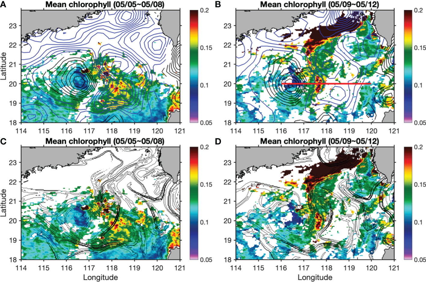
Surface chlorophyll concentration (units: mg m-3) overlaid by SLA (units: m; black contours for positive and blue ones for negative values) in (A, B), and overlaid by FSLE contours larger than 0.1 d-1 in (C, D) during 5-12 May. The red line in (B) denotes the position of the transect for further analysis.
A transect through the edge region between CE1 and CE2 also showed that chlorophyll concentration in the CE was generally higher than that in the AC. The highest chlorophyll was present in the edge region with small negative SLAs and large FSLE values (Figure 3). High strain between eddies may create submesoscale upwelling/downwelling motion that facilitates nutrient transport vertically. Because the surface NSCS in May is generally in a nutrient-limited condition, submesoscale nutrient transport is likely to stimulate phytoplankton growth and generate localized high chlorophyll patches.
Figure 3
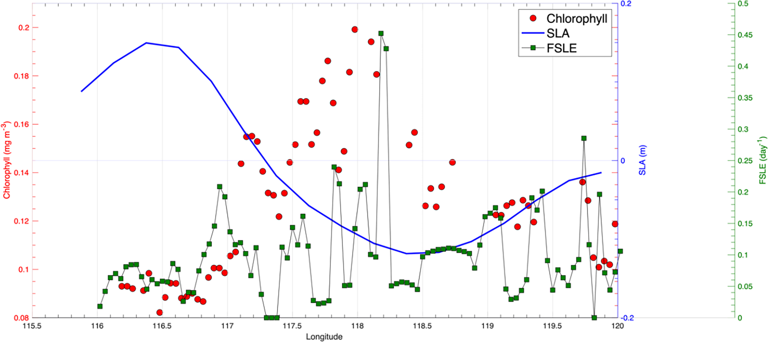
Spatial variability of SLA (units: m), surface chlorophyll concentration (units: mg m-3), and FSLE (units: day-1) along the transect shown in Figure 2B.
To investigate the existence of upwelling, movements of passive particles were tracked in the model. Although the model missed the SLA magnitudes slightly, it reproduced CE1, CE2 and AC1 reasonably well (Figure 4). On 4 May, over 50,000 passive particles were released in the model at 50 m in the area between CE1 and CE2, covering both the core and edge regions (Figure 4). The movements of these particles were tracked over time in the model. These particles were first stretched along the hyperbolic region and then advected away mostly at the eddy edge. Only a relatively small number of particles stayed in the eddy core as it propagated. We tracked those particles that entered the mixed layer after seven days from their release, and found that they were generally the ones released at the eddy edge regions (Figure 5). Consistent with this pattern, the probability of particles staying in the mixed layer during the one-month period is particularly higher at the eddy edge regions (Figure 6).
Figure 4
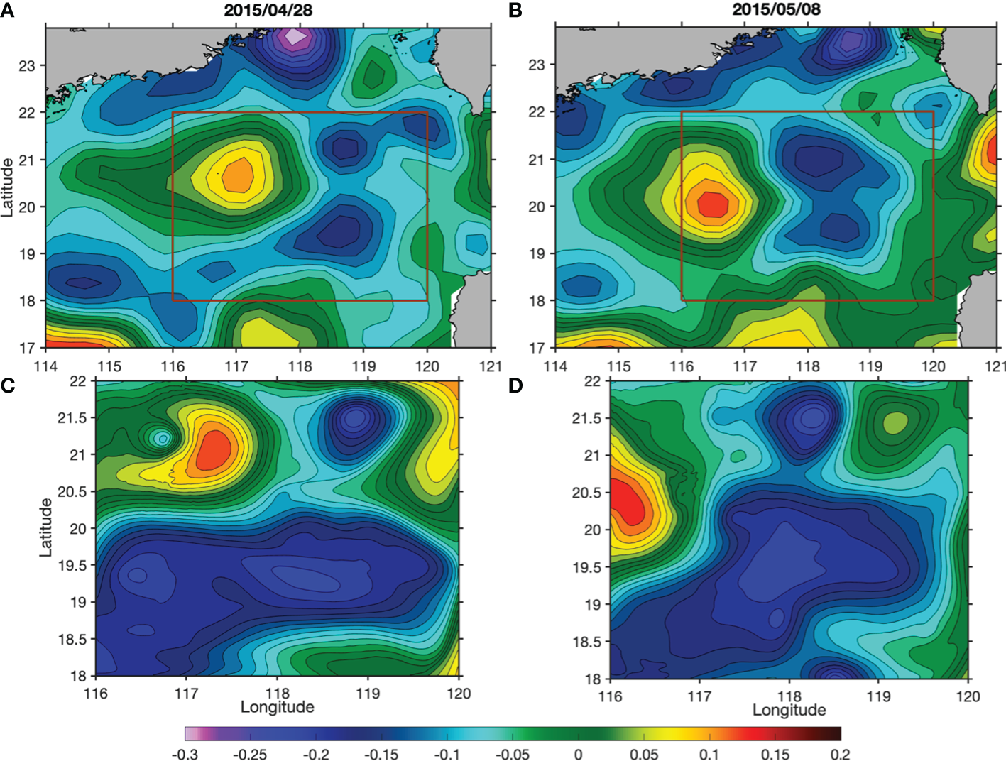
Comparisons of spatial distributions of SLA (units: m) from altimeter data (A, B) and the model outputs (C, D) on 28 April and 8 May. The red rectangles in (A, B) depict the domain of the model.
Figure 5
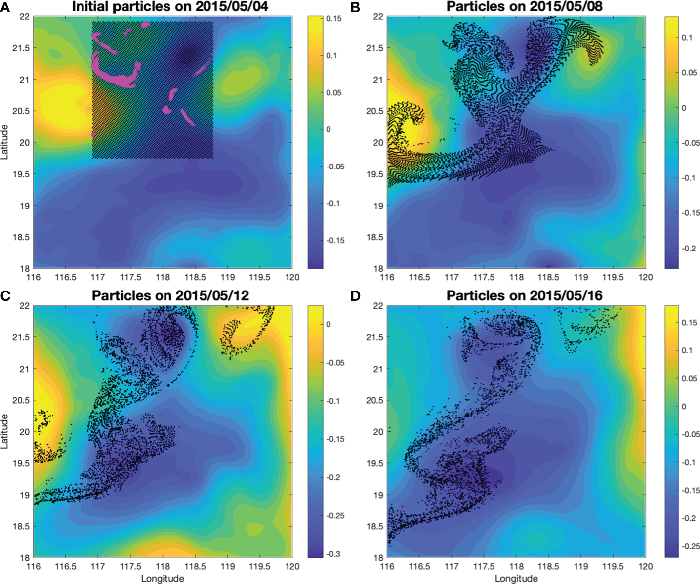
Lagrangian particle releasing results on 04 May (A), 08 May (B), 12 May (C) and 16 May 2015 (D). The particles were released at the surface of a depth of 50 m. The black dots show the particle locations on different days. The shadings are SLA (units: m). The magenta circles in (A) are the particles being brought into the mixed layer 7 days after being released.
Figure 6
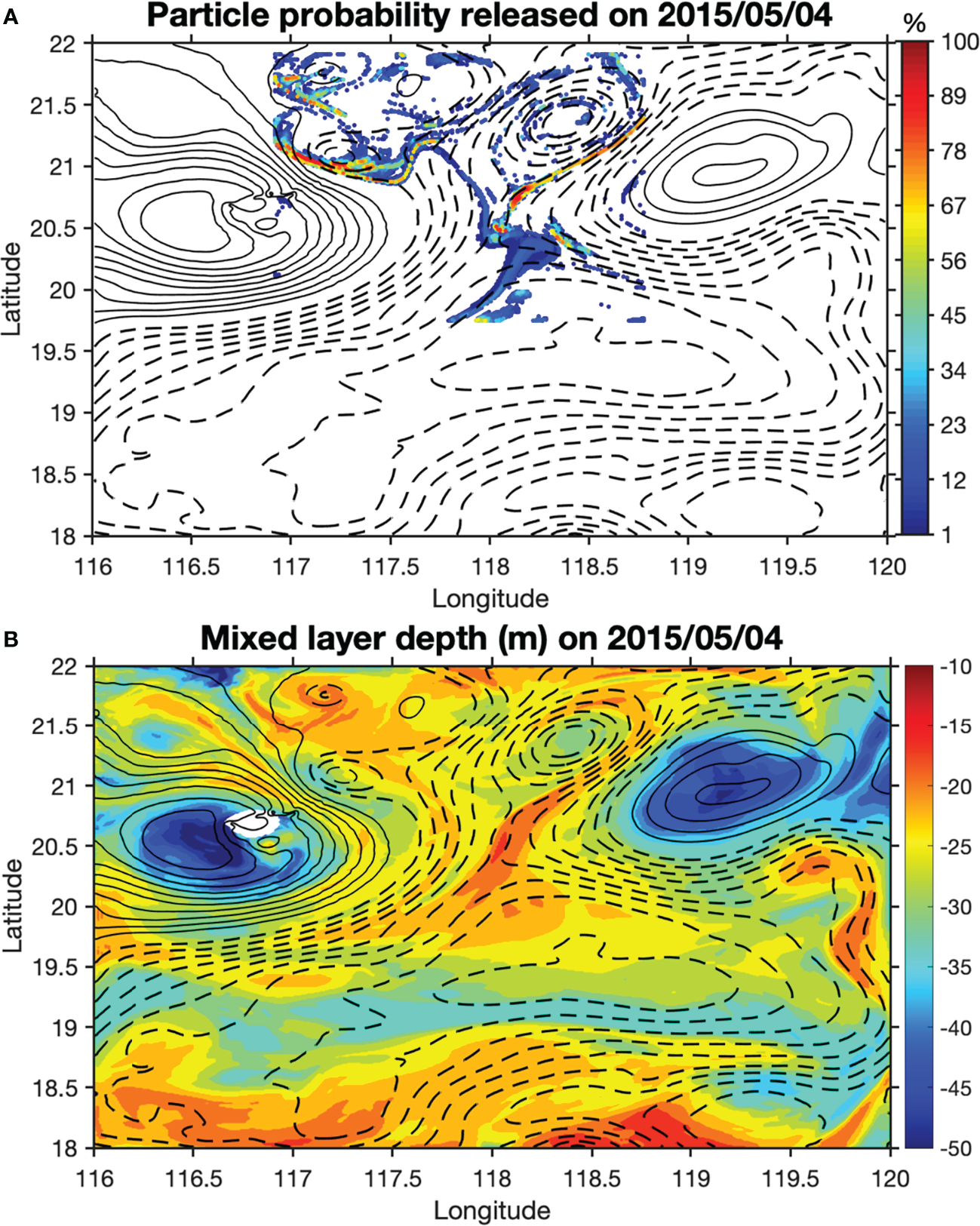
The spatial distribution of particle probability of staying in the mixed layer in May 2015 (A) and the spatial distribution of modeled mixed layer depth (m) on 4 May 2015 (B). The particles were released at 50-m depth on 4 May. The contours are the SLA isolines with solid and dashed lines denoting positive and negative values, respectively.
Driving mechanisms
The submesoscale nutrient transport was further examined in the model. On May 8, the nitrate concentration at 50 m showed localized high patches (Figure 7). These patches were at a submesoscale length scale and present around mesoscale eddies. To examine the physical processes driving these nitrate patches, two cases were chosen. We used two moving boxes (50×50 km) to encompass two nitrate patches and follow their movements (white box for case1, red box for case2).
Figure 7
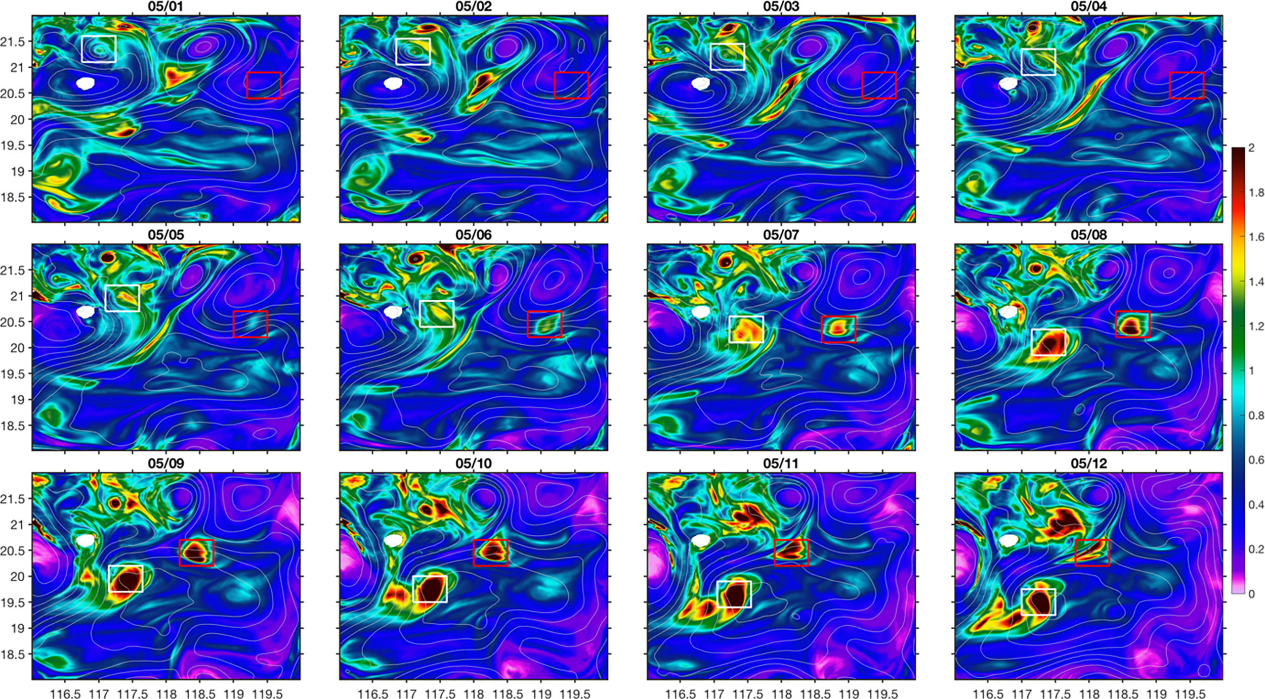
Spatial distributions of nitrate concentration (mmol m-3) at 50 m from the model outputs. The white and red rectangles mark the locations of two high nitrate patches for analysis.
For case1, the high nitrate patch was associated with a coherent submesoscale eddy that can be captured from surface SLA (Figure 7). This eddy has a radius of ~20 km. It was formed near the Dongsha Island, probably related to the current-topography interactions (Zhang et al., 2022). From 5 May, it was advected to the southwest by the current at the edge of mesoscale eddies. This submesoscale eddy associated with high nitrate concentration eventually merged into the mesoscale cyclonic eddy, CE2, providing a significant contribution of nitrate input flux to CE2. While the submesoscale eddy propagated, the distribution of vertical velocity (w) at 80 m displayed a diapole pattern with positive w at the leading edge and negative w at its trailing edge (Figure 8). The similar distribution pattern of current divergence (δ=ux+vy ; where u, v are the velocity components in x, y, i.e., east and north, directions) with positive and negative values corresponding to upwelling and downwelling, respectively, suggests that current divergence is the possible mechanism leading to the upwelling and downwelling processes (Figure 8).
Figure 8
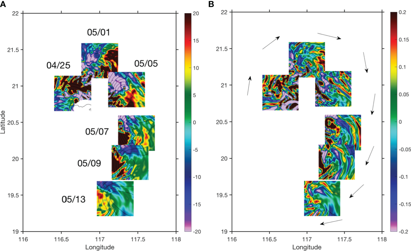
Distributions of vertical velocity (A units: m d-1) at 80 m and normalized current divergence (A) at 50 m following the propagation the submesoscale eddy of case1. The arrows in (B) illustrates the general moving directions of the box.
Following the propagation of the submesoscale eddy, both positive and negative w decreased with time in a similar manner, probably suggesting a connected circulation cell (Figure 9A). Nevertheless, the box-averaged w stayed positive during the eddy propagation, which also drives the positive nitrate flux vertically Figure. The vorticity (ζ=vx−uy ) normalized by the Coriolis frequency (f) indicated that the submesoscale eddy experienced both the developing stage before 29 April and the decay stage afterwards (Figure 9B). During its developing stage, nitrate level at 50 m was relatively stable and it started to increase during its decay stage while propagating (Figure 9C). During its propagation, the net nitrate flux was generally positive due to the relatively smaller negative horizontal flux, which resulted in the accumulation of nitrate concentration in the upper layer (Figure 9D). Following the movement of the submesoscale eddy, modeled mean chlorophyll concentration in the upper 50 m increased from 0.1 mg m-3 to 0.24 mg m-3, which was in a similar magnitude as the satellite data.
Figure 9
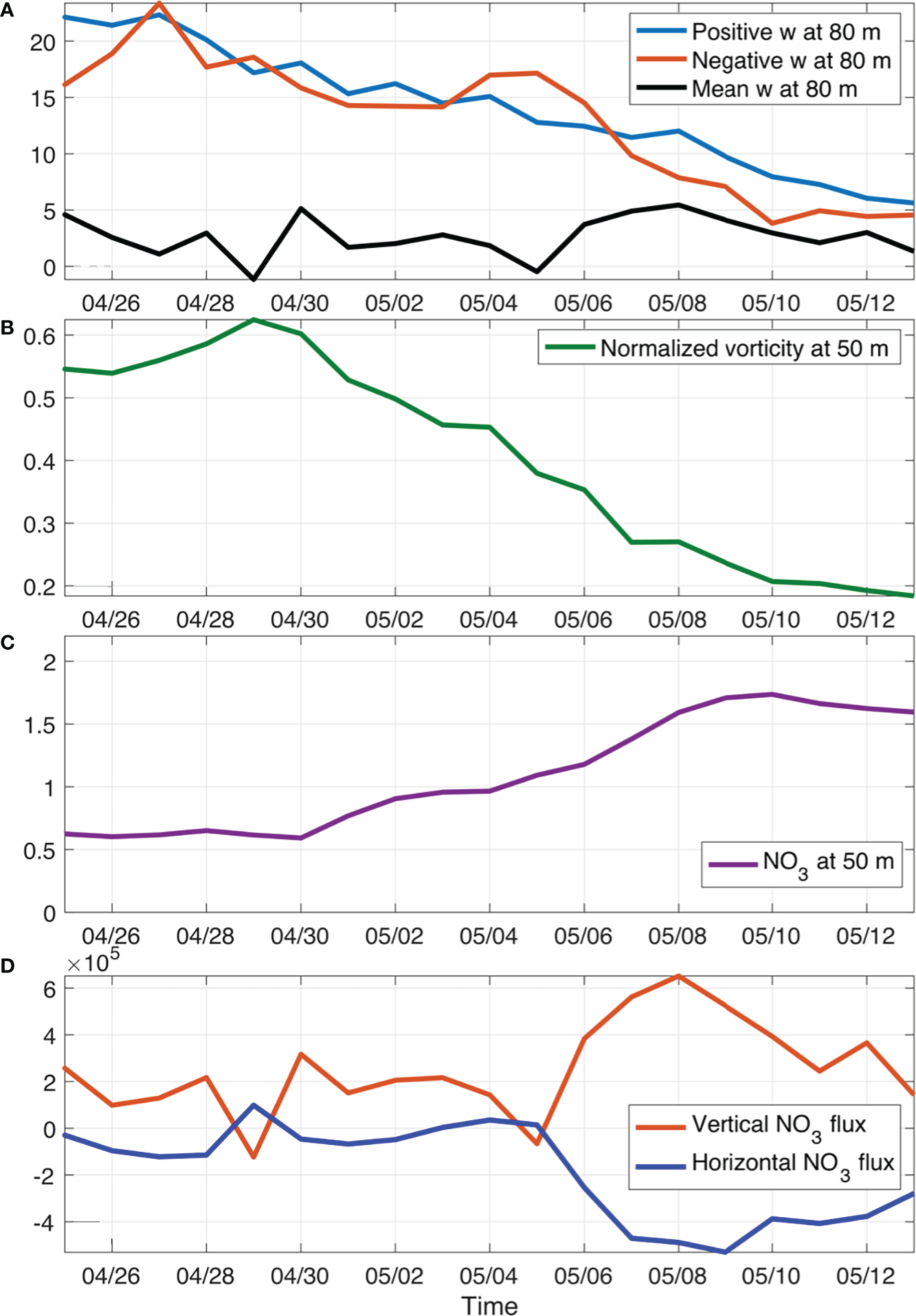
Temporal variations of box-averaged vertical velocities (A; units: m d-1), normalized vorticity by f(B), nitrate concentration (C; mmol m-3), and nitrate fluxes (D; units: mmol s-1) following the movement of case1 patch. Here, the horizontal nitrate flux was calculated from surface to 80 m and the vertical flux was calculated at 80 m.
For case2, the high nitrate patch that can reach higher than 2.0 mmol m-3 was not associated with any coherent circulation structures (red box in Figure 7). It showed up on 5 May and was eventually stretched away by the horizontal current between mesoscale eddies. The box averaged nitrate concentration showed a similar temporal pattern (Figure 10A). The increase of nitrate from 5 May was induced by the positive net nitrate flux (horizontal plus vertical flux) into the box that was largely driven by the increase of positive w (Figures 10B, C). On 4 May, there was an increase of north-south density gradient (Figure 10E), which can consequently lead to enhanced horizontal strain () and further induce secondary circulation with strong upward water motions (Figures 10B, D). This mechanism is consistent with frontal dynamics. We further composited the w at 80 m from 6 May to 12 May when the case2 patch moved generally in a zonal direction along the front between a mesoscale anticyclonic eddy in the north and a mesoscale cyclonic eddy in the south. The spatial distribution pattern of composited w demonstrated positive values in the north and negative values in the south in correspondence to the low density in the north and high density in the south, respectively (Figure 11). Therefore, the elevated nitrate concentration in case2 was mainly induced by the frontal dynamics. The modeled chlorophyll change in the case2 patch generally followed the change of nitrate concentration over time.
Figure 10
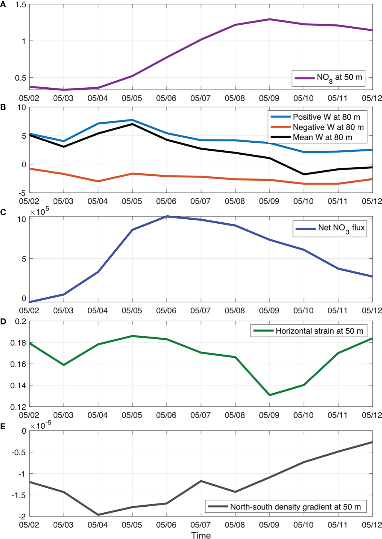
Temporal variations of box-averaged nitrate concentration (A; unit: mmol m-3), vertical velocities (B; units: m d-1), net nitrate advection flux (C; unit: mmol s-1), normalized horizontal strain by f(D), and north-south density gradient (E; unit: kg m-4) of case2 patch.
Figure 11
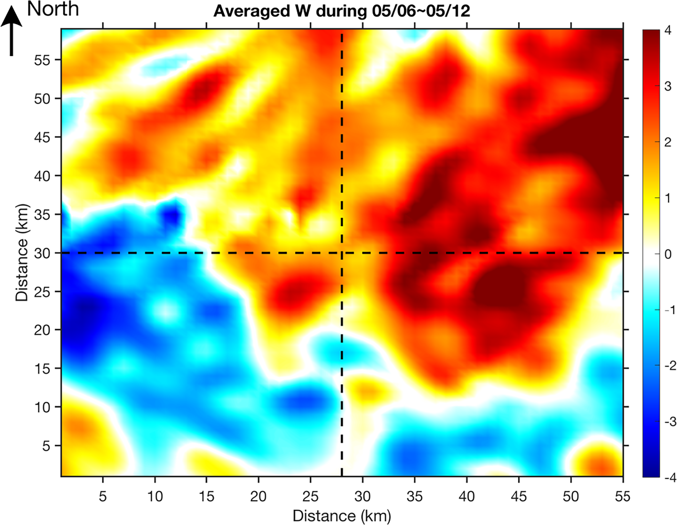
Composted mean of modeled vertical velocity (unit: m d-1) at 80 m for case2 during 6 May~12 May, 2015.
Discussion and conclusions
Mesoscale eddies are known to induce perturbations in biogeochemistry in the eddy core through mesoscale dynamics. In addition to mesoscale responses, high-resolution chlorophyll images often show patchy distribution patterns that vary over a distance of a few kilometers at a temporal scale of days, which are suggested to link to submesoscale dynamics. At submesoscale, the spatial and temporal variations of tracers such as phytoplankton chlorophyll is often related (Mahadevan, 2016). Thus, to resolve submesoscale structures, both spatial and temporal resolutions need to be fine enough.
Two mechanisms have been previously suggested to generate submesoscale structures. One is the mesoscale-driven frontogenesis (Lapeyre et al., 2006; Mahadevan and Tandon, 2006), and the other is the mixed-layer instability (MLI; Boccaletti et al., 2007). The vertical scale of MLI is the mixed layer depth. The mixed layer depth during the study period was generally shallower than 40 m, except in the regions where anticyclonic eddies were present (Figure 6B). From the model results, we found strong fluctuations of isopycnals and upwelling/downwelling motions below the mixed layer. These fluctuations of isopycnals were conspicuously observed in the edge region between mesoscale eddies, where enhanced shear and strain can sharpen existing horizontal density gradient and give rise to submesoscale upwelling/downwelling motions. It is thus likely that the submesoscale processes were induced by frontogenesis and baroclinic instabilities (Ramachandran et al., 2014; Zhang et al., 2021). Other studies also indicated that the frontogenesis plays a key role in generating submesoscale processes in the SCS (Zhong et al., 2017).
By simplifying the omega equation in a frontal region, we can obtain its two-dimensional version, that is,
This omega equation is derived by assuming that the x variation (along the front) in the data is much smaller than its y variation (across the front). It states that mesoscale flow can drive the growth of submesoscale density gradient associated with vertical velocity. With further simplification of this equation, Legal et al. (2007) derived an expression indicating the robust correlation between vertical velocity and density anomaly. It is consistent with the findings of this study, in which intense vertical velocity was illustrated by particle trajectories between eddies. The modeling results for submesoscale case2 have shown that such vertical motion is often linked with the vertical transport of tracers, such as nutrients, consistent with previous studies (Lévy et al., 2001; Lapeyre and Klein, 2006).
In addition, the modeling results showed that submesoscale eddy could be another mechanism inducing strong vertical nutrient transport at submesoscale. Although case1 was not generated at the eddy edge, it was carried away by the flow around the mesoscale eddy after formation. During its movements, divergence induced upwelling at the leading edge kept injecting nutrient from subsurface to the upper layer. Previous satellite study in the western SCS has observed such small-scale eddies associated with high surface chlorophyll concentrations (Liu et al., 2015). The submesoscale eddy could also be a potential nutrient source to mesoscale eddy once they merge together.
Biological responses to submesoscale processes are more complicated than physical tracers. Nutrients upwelled from subsurface can be taken up by different phytoplankton species that are further modulated by ecosystem dynamics and other biogeochemical processes, which are all subject to different temporal scales (Lévy et al., 2018). The short time scales associated with strong submesoscale vertical nutrient injections and the biological response time favour dominance by the large phytoplankton size class (diatoms) of the model (Figure 12; Lévy et al., 2012; Guo et al., 2022). Different physical dynamics between mesoscale and submesoscale processes can thus lead to spatial and temporal heterogeneities in community structure and ecosystem dynamics (d’Ovidio et al., 2010; Lévy et al., 2012; Clayton et al., 2014; Mousing et al., 2016; Clayton et al., 2017). Moreover, the intensity of nutrient injection induced by submesoscale processes is also determined by the background nutricline depths that are set by mesoscale or large-scale processes. Consequently, regions with high physical straining and stretching are not always associated with enhanced total chlorophyll concentration (e.g., Guo et al., 2022).
Figure 12
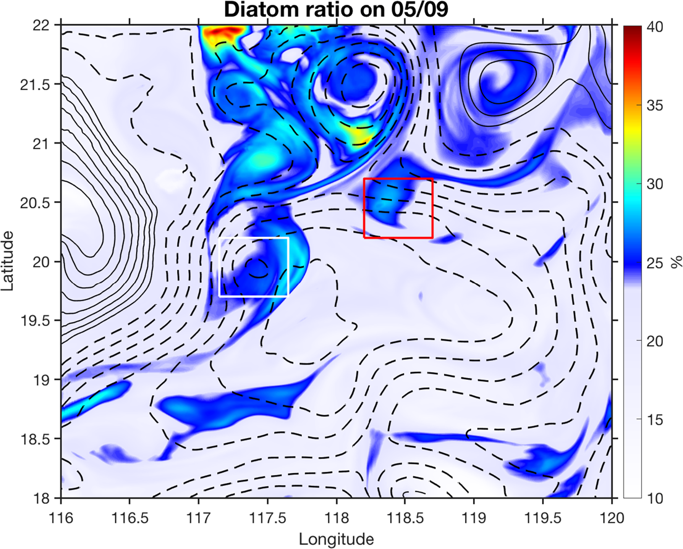
Modeled diatom ratio (%) in total phytoplankton averaged in the upper 50 m on 9 May 2015. The red and white rectangles depict two submesoscale nitrate patches. The contours are the SLA isolines with solid and dashed lines denoting positive and negative values, respectively.
In conclusion, with a high-resolution coupled model, we examined submesoscale processes between mesoscale eddies in the NSCS. By calculating the FSLE from altimeter data and tracking Lagrangian particles in the three-dimensional model, the submesoscale upwelling motion was revealed between eddies. We found that both frontal dynamics and submesoscale coherent eddies can inject subsurface nutrients into the upper layer, stimulate phytoplankton growth, and alter community structure. As the coupled model didn’t include data assimilation, model discrepancies were found in simulating the strength and locations of mesoscale and submesoscale features. This study can serve as a process-orientated study to investigate potential dynamics and impacts of submesoscale features on biology. This study shows the strong physical-biological links at submesoscale in the NSCS, highlighting the importance of submesoscale processes on marine ecosystem and the need for high-resolution observations.
Funding
This research was supported by the Key Special Project for Introduced Talents Team of Southern Marine Science and Engineering Guangdong Laboratory (Guangzhou) (GML2019ZD0305) and the National Natural Science Foundation of China (41890805, 41730536).
Acknowledgments
The Ocean Color Climate Change Initiative (OC-CCI, Version 3.1) data were obtained from http://www.esa-oceancolour-cci.org/. The Cross-Calibrated Multi-Platform (CCMP) Version-2.0 data were obtained from www.remss.com. Six-hourly NCEP/NCAR Reanalysis surface forcing data were obtained from https://www.esrl.noaa.gov/psd/. The SLA and FSLE data were obtained from https://www.aviso.altimetry.fr/.
Publisher’s note
All claims expressed in this article are solely those of the authors and do not necessarily represent those of their affiliated organizations, or those of the publisher, the editors and the reviewers. Any product that may be evaluated in this article, or claim that may be made by its manufacturer, is not guaranteed or endorsed by the publisher.
Statements
Data availability statement
The raw data supporting the conclusions of this article will be made available by the authors, without undue reservation.
Author contributions
Conceptualization: PX, WM; Methodology: LG, PX. Writing: PX. Review and editing: LG, WM. Funding acquisition: PX. All authors contributed to the article and approved the submitted version.
Conflict of interest
The authors declare that the research was conducted in the absence of any commercial or financial relationships that could be construed as a potential conflict of interest.
References
1
Boccaletti G. Ferrari R. Fox-Kemper B. (2007). Mixed layer instabilities and restratification. J. Phys. Oceanogr.37, 2228–2250. doi: 10.1175/JPO3101.1
2
Chai F. Dugdale R. C. Peng T. H. Wilkerson F. P. Barber R. T. (2002). One dimensional ecosystem model of the equatorial pacific upwelling system, part I: Model development and silicon and nitrogen cycle. Deep. Sea. Res. II.49, 2713–2745. doi: 10.1016/S0967-0645(02)00055-3
3
Chelton D. B. Gaube P. Schlax M. G. Early J. J. Samelson R. M. (2011). The influence of nonlinear mesoscale eddies on near-surface oceanic chlorophyll. Science334 (6054), 328–332. 10.1126/science.1208897
4
Chen Y.-L. Chen H.-Y. Lin I.-I. Lee M.-A. Chang J. (2007). Effects of cold eddy on phytoplankton production and assemblages in Luzon strait bordering the south China Sea. J. Oceanogr.671–683, 63. doi: 10.1007/s10872-007-0059-9
5
Clayton S. Dutkiewicz S. Jahn O. Hill C. Heimbach P. Follows M. J. (2017). Biogeochemical versus ecological consequences of modeled ocean physics. Biogeosciences14, 2877–2889. doi: 10.5194/bg-14-2877-2017
6
Clayton S. Nagai T. Follows M. J. (2014). Fine scale phytoplankton community structure across the kuroshio front. J. Plankton. Res.36 (4), 1017–1030. doi: 10.1093/plankt/fbu020
7
Dong J. Zhong Y. (2018). The spatiotemporal features of submesoscale processes in the northern south China Sea. Acta Oceanol. Sin.37 (11), 8–18. 10.1007/s13131-018-1277-2
8
Döös K. (1995). Interocean exchange of water masses. J. Geophys. Res.100, 13499–13514. doi: 10.1029/95JC00337
9
d’Ovidio F. De Monte S. Alvain S. Dandonneau Y. Lévy M. (2010). Fluid dynamical niches of phytoplankton types. Proc. Natl. Acad. Sci.107 (43), 18366. doi: 10.1073/pnas.1004620107
10
d’Ovidio F. Fernandez V. Hernandez-Garca E. Lopez C. (2004). Mixing structures in the Mediterranean Sea from finite-size lyapunoov exponent. Geophys. Res. Lett.31, L17203. doi: 10.1029/2004GL020328
11
d’Ovidio F. Isern-Fontanet J. López C. Hernández-García E. García-Ladona E. (2009). Comparison between eulerian diagnostics and finite-size lyapunov exponents computed from altimetry in the Algerian basin. Deep-Sea. Res. I.56, 15–31. doi: 10.1016/j.dsr.2008.07.014
12
Estapa M. L. Siegel D. A. Buesseler K. O. Stanley R. H. R. Lomas M. W. Nelson N. B. (2015). Decoupling of net community and export production on submesoscales in the Sargasso Sea. Global Biogeochem. Cycles.29, 1266–1282. doi: 10.1002/2014GB004913
13
Falkowski P. G. Ziemann D. Kolber Z. Bienfang P. K. (1991). Role of eddy pumping in enhancing primary production in the ocean. Nature352, 55–58. doi: 10.1038/352055a0
14
Frenger I. Bianchi D. Stührenberg C. Oschlies A. Dunne J. Deutsch C. et al . (2018). Biogeochemical role of subsurface coherent eddies in the ocean: Tracer cannonballs, hypoxic storms, and microbial stewpots? Global Biogeochem. Cycles.32 (2), 226–249. doi: 10.1002/2017GB005743
15
Gan J. Li H. Curchitser E. N. Haidvogel D. B. (2006). Modeling south China Sea circulation. response to seasonal forcing regimes. J. Geophys. Res.111, C06034. doi: 10.1029/2005JC003298
16
Gaube P. Chelton D. B. Strutton P. G. Behrenfeld M. J. (2013). Satellite observations of chlorophyll, phytoplankton biomass, and ekman pumping in nonlinear mesoscale eddies. J. Geophys. Res.: Oceans118, 6349–6370. doi: 10.1002/2013JC009027
17
Gula J. Blacic T. M. Todd R. E. (2019). Submesoscale coherent vortices in the gulf stream. Geophysical. Res. Lett.46, 2704–2714. doi: 10.1029/2019GL081919
18
Guo M. Chai F. Xiu P. Li S. Rao S. (2015). Impacts of mesoscale eddies in the south China Sea on biogeochemical cycles. Ocean. Dynamics.65, 1335–1352. doi: 10.1007/s10236-015-0867-1
19
Guo M. Xiu P. Xing X. (2022). Oceanic fronts structure phytoplankton distributions in the central south Indian ocean. J. Geophys. Res.: Oceans.127, e2021JC017594. doi: 10.1029/2021JC017594
20
He Q. Zhan H. Cai S. Li Z. (2016). Eddy effects on surface chlorophyll in the northern south China Sea: Mechanism investigation and temporal variability analysis. Deep-Sea. Res. I.112, 25–36. doi: 10.1016/j.dsr.2016.03.004
21
Huang B. Hu J. Xu H. Cao Z. Wang D. (2010). Phytoplankton community at warm eddies in the northern south China Sea. Deep-Sea. Res. II.57, 1792–1798. doi: 10.1016/j.dsr2.2010.04.005
22
Klein P. Lapeyre G. (2009). The ocean vertical pump induced by mesoscale and submesoscale turbulence. Annu. Rev. Mar. Sci.1, 351–375. doi: 10.1146/annurev.marine.010908.163704
23
Lapeyre G. Klein P. (2006). Impact of the small-scale elongated filaments on the oceanic vertical pump. J. Mar. Res.64, 835–851. doi: 10.1357/002224006779698369
24
Lapeyre G. Klein P. Hua B. L. (2006). Oceanic restratification forced by surface frontogenesis. J. Phys. Oceanogr.36, 1577–1590. doi: 10.1175/JPO2923.1
25
Lavender S. Jackson T. Sathyendranath S. (2015). The ocean color climate change initiative. Ocean. Challenge.21 (1).
26
Legal C. Klein P. Treguier A.-M. Paillet J. (2007). Diagnosis of the vertical motions in a mesoscale stirring region. J. Phys. Oceanogr.37 (5), 1413–1424. doi: 10.1175/JPO3053.1
27
Lehahn Y. d’Ovidio F. Lévy M. Heifetz E. (2007). Stirring of the northeast Atlantic spring bloom: A Lagrangian analysis based on multisatellite data. J. Geophys. Res.112, C08005. doi: 10.1029/2006JC003927
28
Lévy M. Ferrari R. Franks P. J. Martin A. P. Rivière P. (2012). Bringing physics to life at the submesoscale. Geophys. Res. Lett.39, L14602. doi: 10.1029/2012GL052756
29
Lévy M. Franks P. J. Smith K. S. (2018). The role of submesoscale currents in structuring marine ecosystems. Nat. Commun.9, 4758. doi: 10.1038/s41467-018-07059-3
30
Lévy M. Klein P. Treguier A.-M. (2001). Impact of sub-mesoscale physics on production and subduction of phytoplankton in an oligotrophic regime. J. Mar. Res.59, 535–565. doi: 10.1357/002224001762842181
31
Liu K. K. Chao S. Y. Shaw P. T. Gong G. C. Chen C. C. Tang T. Y. (2002). Monsoon-forced chlorophyll distribution and primary production in the south China Sea: observations and a numerical study. Deep. Sea. Res. I.49, 1387–1412. doi: 10.1016/S0967-0637(02)00035-3
32
Liu G. He Y. Shen H. Qiu Z. (2010). Submesoscale activity over the shelf of the northern south China Sea in summer: simulation with an embedded model. Chin. J. Oceanography. Limnology.28 (5), 1073–1079. doi: 10.1007/s00343-010-0030-2
33
Liu F. Tang S. Chen C. (2015). Satellite observations of the small-scale cyclonic eddies in the western south China Sea. Biogeosciences12, 299–305. doi: 10.5194/bg-12-299-2015
34
Liu F. Tang S. Huang R. Yin K. (2017). The asymmetric distribution of phytoplankton in anticyclonic eddies in the western south China Sea. Deep-Sea. Res. I.120, 29–38. doi: 10.1016/j.dsr.2016.12.010
35
Li C. Zhang Z. Zhao W. Tian J. (2017). A statistical study on the subthermocline submesoscale eddies in the northwestern pacific ocean based on argo data. J. Geophys. Res.: Oceans.122, 3586–3598. doi: 10.1002/2016JC012561
36
Lukas R. Santiago-Mandujano F. (2001). Extreme water mass anomaly observed in the Hawaii ocean time-series. Geophys. Res. Lett.28, 2931–2934. doi: 10.1029/2001GL013099
37
Mahadevan A. (2016). The impact of submesoscale physics on primary productivity of plankton. Annu. Rev. Mar. Sci.8, 17.1–17.24. doi: 10.1146/annurev-marine-010814-015912
38
Mahadevan A. D'Asaro E. Perry M.-J. Lee C. (2012). Eddy-driven stratification initiates north Atlantic spring phytoplankton blooms. Science3376090), 54–58. doi: 10.1126/science.1218740
39
Mahadevan A. Tandon A. (2006). An analysis of mechanisms for submesoscale vertical motion at ocean fronts. Ocean. Model.14, 241–256. doi: 10.1016/j.ocemod.2006.05.006
40
Martin A. P. Richards K. J. (2001). Mechanisms for vertical nutrient transport within a north Atlantic mesoscale eddy. Deep-Sea. Res. II.48, 757–773. doi: 10.1016/S0967-0645(00)00096-5
41
Ma W. Xiu P. Chai F. Li H. (2019). Seasonal variability of the carbon export in the central south China Sea. Ocean. Dynamics.69 (8), 955–966. doi: 10.1007/s10236-019-01286-y
42
McGillicuddy D. J. Anderson L. A. Bates N. R. Bibby T. Buesseler K. O. Carlson C. A. et al . (2007). Eddy/wind interactions stimulate extraordinary mid-ocean plankton blooms. Science316, 1021–1026. doi: 10.1126/science.1136256
43
McGillicuddy D. J. Robinson A. R. Siegel D. A. Jannasch H. W. Johnson R. Dickey T. D. et al . (1998). Influence of mesoscale eddies on new production in the Sargasso Sea. Nature394, 263–266. doi: 10.1038/28367
44
McWilliams J. C. (1985). Submesoscale, coherent vortices in the ocean. Rev. Geophysics.23, 165–182. doi: 10.1029/RG023i002p00165
45
Mousing E. A. Richardson K. Bendtsen J. Cetinić I. Perry M. J. (2016). Evidence of small-scale spatial structuring of phytoplankton alpha- and beta-diversity in the open ocean. J. Ecol.104 (6), 1682–1695. doi: 10.1111/1365-2745.12634
46
Ning X. Chai F. Xue H. Cai Y. Liu C. Zhu G. et al . (2004). Physical-biological oceanographic coupling influencing phytoplankton and primary production in the south China Sea. J. Geophys. Res.109, C10005. doi: 10.1029/2004JC002365
47
Ni Q. Zhai X. Wilson C. Chen C. Chen D. (2021). Submesoscale eddies in the south China. Geophys. Res. Lett.48, e2020GL091555. doi: 10.1029/2020GL091555
48
Omand M. M. D'Asaro E. A. Lee C. M. Perry M. J. Briggs N. Cetinic I. et al . (2015). Eddy-driven subduction exports particulate organic carbon from the spring bloom. Science348, 222–225. doi: 10.1126/science.1260062
49
Qiu C. Mao H. Liu H. Xie Q. Yu J. Su D. et al . (2019). Deformation of a warm eddy in the northern south China Sea. J. Geophys. Res.: Oceans.124, 5551–5564. doi: 10.1029/2019JC015288
50
Ramachandran S. Tandon A. Mahadevan A. (2014). Enhancement in vertical fluxes at a front by mesoscale- submesoscale coupling. J. Geophys. Res.: Oceans.119, 8495–8511. doi: 10.1002/2014JC010211
51
Shu Y. Xiu P. Xue H. Yao J. Yu J. (2016). Glider-observed anticyclonic eddy in northern south China Sea. Aquat. Ecosyst. Health Manage.19, 233–241. doi: 10.1080/14634988.2016.1208028
52
Siegel D. A. Peterson P. McGillicuddy D. J. Maritorena S. Nelson N. B. (2011). Bio-optical footprints created by mesoscale eddies in the Sargasso Sea. Geophys. Res. Lett.38, L13608. doi: 10.1029/2011GL047660
53
Wang L. Huang B. Laws E. A. Zhou K. Liu X. Xie Y. et al . (2018). Anticyclonic eddy edge effects on phytoplankton communities and particle export in the northern south China Sea. J. Geophys. Res.123 (11), 7632–7650. doi: 10.1029/2017JC013623
54
Xiu P. Chai F. (2011). Modeled biogeochemical responses to mesoscale eddies in the south China Sea. J. Geophys. Res. Oceans.116, C10006. doi: 10.1029/2010JC006800
55
Xiu P. Dai M. Chai F. Zhou K. Zeng L. Du C. (2019). On contributions by wind-induced mixing and eddy pumping to interannual chlorophyll variability during different ENSO phases in the northern south China Sea. Limnol. Oceanogr.64, 503–514. doi: 10.1002/lno.11055
56
Zhang Z. Tian J. Qiu B. Zhao W. Chang P. Wu D. et al . (2016). Observed 3D structure, generation, and dissipation of oceanic mesoscale eddies in the south China Sea. Sci. Rep.6, 24349. doi: 10.1038/srep24349
57
Zhang X. Zhang Z. McWilliams J. C. Sun Z. Zhao W. Tian J. (2022). Submesoscale coherent vortices observed in the northeastern south China Sea. J. Geophys. Res.: Oceans.127, e2021JC018117. doi: 10.1029/2021JC018117
58
Zhang Z. Zhang X. Qiu B. Zhao W. Zhou C. Huang X. et al . (2021). Submesoscale currents in the subtropical upper ocean observed by long-term high-resolution mooring arrays. J. Phys. Oceanogr.51, 187–206. doi: 10.1175/JPO-D-20-0100.1
59
Zhong Y. Bracco A. Tian J. Dong J. Zhao W. Zhang Z. (2017). Observed and simulated submesoscale vertical pump of an anticyclonic eddy in the south China Sea. Sci. Rep.7, 44011. doi: 10.1038/srep44011
60
Zhou K. Dai M. Kao S.-J. Wang L. Xiu P. Chai F. et al . (2013). Apparent enhancement of 234Th-based particle export associated with anticyclonic eddies. Earth Planetary. Sci. Lett.381, 198–209. doi: 10.1016/j.epsl.2013.07.039
Summary
Keywords
submesoscale process, mesoscale eddy, phytoplankton chlorophyll, nutrient flux, phytoplankton community
Citation
Xiu P, Guo L and Ma W (2022) Modelling the influence of submesoscale processes on phytoplankton dynamics in the northern South China Sea. Front. Mar. Sci. 9:967678. doi: 10.3389/fmars.2022.967678
Received
13 June 2022
Accepted
20 July 2022
Published
08 August 2022
Volume
9 - 2022
Edited by
Dilip Kumar Jha, National Institute of Ocean Technology, India
Reviewed by
Pankaj Verma, National Institute of Ocean Technology, India; Nithyanandam Marimuthu, Zoological Survey of India, India; Mehmuna Begum, National Centre for Coastal Research, India
Updates
Copyright
© 2022 Xiu, Guo and Ma.
This is an open-access article distributed under the terms of the Creative Commons Attribution License (CC BY). The use, distribution or reproduction in other forums is permitted, provided the original author(s) and the copyright owner(s) are credited and that the original publication in this journal is cited, in accordance with accepted academic practice. No use, distribution or reproduction is permitted which does not comply with these terms.
*Correspondence: Wentao Ma, wtma@sio.org.cn
This article was submitted to Marine Pollution, a section of the journal Frontiers in Marine Science
Disclaimer
All claims expressed in this article are solely those of the authors and do not necessarily represent those of their affiliated organizations, or those of the publisher, the editors and the reviewers. Any product that may be evaluated in this article or claim that may be made by its manufacturer is not guaranteed or endorsed by the publisher.