Abstract
Classifying the ocean into regions with distinct biogeochemical or physical properties may enhance our interpretation of ocean processes. High-resolution satellite-derived products provide valuable data to address this task. Notwithstanding, no regionalization at a regional scale has been attempted for the coastal and open oceans of British Columbia (BC) and Southeast Alaska (SEA), which host essential habitats for several ecologically, culturally, and commercially important species. Across this heterogeneous marine domain, phytoplankton are subject to dynamic ocean circulation patterns and atmosphere-ocean-land interactions, and their variability, in turn, influences marine food web structure and function. Regionalization based on phytoplankton biomass patterns along BC and SEA’s coastal and open oceans can be valuable in identifying pelagic habitats and representing a baseline for assessing future changes. We developed a two-step classification procedure, i.e., a Self-Organizing Maps (SOM) analysis followed by the affinity propagation clustering method, to define ten bioregions based on the seasonal climatology of high-resolution (300 m) Sentinel-3 surface chlorophyll-a data (a proxy for phytoplankton biomass), for the period 2016-2020. The classification procedure allowed high precision delineation of the ten bioregions, revealing separation between off-shelf bioregions and those in neritic waters. Consistent with the high-nutrient, low-chlorophyll regime, relatively low values of phytoplankton biomass (< 1 mg/m3) distinguished off-shelf bioregions, which also displayed, on average, more prominent autumn biomass peaks. In sharp contrast, neritic bioregions were highly productive (>> 1 mg/m3) and characterized by different phytoplankton dynamics. The spring phytoplankton bloom onset varied spatially and inter-annually, with substantial differences among bioregions. The proposed high-spatial-resolution regionalization constitutes a reference point for practical and more extensive implementation in understanding the spatial dynamics of the regional ecology, data-driven ocean observing systems, and objective regional management.
1 Introduction
Despite their highly dynamic nature, physical complexity, and rich biological activity, it is widely accepted that oceans can be partitioned into biogeographic provinces (Reygondeau and Dunn, 2019). The designation of provinces (also called ecological regions or bioregions) identifies coherent and relatively homogeneous biogeochemical regions with observable boundaries. Overall, regionalization is a valuable strategy for characterizing surface ocean variability, testing ecological hypotheses, contextualizing observations, and implementing practical and spatially relevant management and conservation programs (Krug et al., 2017; Reygondeau and Dunn, 2019).
In understanding ocean variability and implementing effective management, regionalization can be helpful for spatially constraining biological processes, including phytoplankton dynamics in response to environmental forcing. Phytoplankton biomass is a powerful indicator of productivity and ecosystem functioning on global and regional scales (Racault et al., 2014). One crucial dynamic is seasonality (or phenology) which can cause an imbalance between trophic levels with consequences for the marine ecosystem (Platt et al., 2007; Asch et al., 2019). Not surprisingly, the importance of phytoplankton and zooplankton phenology to fish stocks have been captured in the match-mismatch and other mechanistic hypotheses (Platt et al., 2003; Sydeman and Bograd, 2009). It is widely recognized that a warming climate may exacerbate phenological mismatches among trophic levels (Edwards and Richardson, 2004), underscoring the importance of phenology when considering ocean regionalization.
The Northeast Pacific is among the world marine regions where ocean surface temperatures have changed most rapidly in the past fifty years (Hobday and Pecl, 2014), and over the last decade, it has experienced increasing marine heatwaves (Di Lorenzo and Mantua, 2016; Amaya et al., 2020), with considerable implications for biomass decrease and shifts in the biogeography of fish stocks (Cheung and Frölicher, 2020; Laurel and Rogers, 2020). However, it has been suggested that upper ocean temperature may serve as a proxy for anomalies in other physical variables, and it is thus not the sole or primary cause of the observed biological variability (Mackas et al., 2007). Knowing the phytoplankton seasonality more accurately, especially in highly dynamic marine ecosystems, is necessary to assess whether higher trophic levels can find sufficient prey across the annual cycles, including during critical life-history stages (Platt et al., 2003; Platt et al., 2007). Along the coastal oceans of British Columbia (BC) and Southeast Alaska (SEA), several studies have examined the match/mismatch dynamics among both lower (i.e., phytoplankton and zooplankton) and upper trophic levels (i.e., fish populations) and their connection to changes in the physical environment (e.g., Mackas et al., 2013; Schweigert et al., 2013; Malick et al., 2015; Perry et al., 2021; Tommasi et al., 2021). More recently, Suchy et al. (2022) found that early/late spring phytoplankton blooms (due to higher/lower mean annual sea surface temperature) result in a mismatch with the phenology of larger crustacean zooplankton, resulting in lower overall crustacean biomass available for the higher trophic levels. The outcomes from these studies have highlighted how knowledge of regional patterns in ocean conditions is essential to understanding the response of regional fish stocks to changes in the pelagic ocean and the cumulative effects on species that migrate between different habitats (Espinasse et al., 2020; Shelton et al., 2021). In this context, delineating marine regions based on phytoplankton biomass patterns along BC and SEA’s coastal oceans is of value in identifying their heterogeneity, defining pelagic habitats, and representing a baseline for assessing future changes.
Due to their ecological relevance, the shapes of seasonal phytoplankton cycles (extracted from chlorophyll-a time series – a proxy for phytoplankton biomass) are commonly used to establish connections between physical changes in the environment and biological productivity and characterize global to regional biogeography, frequently using satellite data (e.g., Foukal and Thomas, 2014; Kheireddine et al., 2021). Indeed, while in situ observations can provide fine-scale and vertically resolved information, satellite-based oceanographic data, although limited to the ocean’s top layers, offers a synoptic view of the ocean, both spatially and temporally, allowing for systematic coverage of seasonality across highly dynamic areas (Foukal and Thomas, 2014; Huot et al., 2019). Previous studies have used coarse spatial resolution (i.e., ≥ 1 km) satellite data and global retrieval algorithms to examine the spatiotemporal variability of chlorophyll-a along the continental margin of the Northeast Pacific and its relationship with local and basin-scale changes in the environment (e.g., Ware and Thomson, 2005; Jackson et al., 2015; Suchy et al., 2019). However, none of these studies used an objective approach to categorize this region but employed grid cells (i.e., square) or predefined polygons when considering spatial variation. An objective regionalization approach allows identifying ecologically meaningful regional scale partitions for the coastal oceans of BC and SEA for the first time.
In this regard, our goal was to provide a regional biogeochemical partitioning that minimizes subjectivity and can be refined and continuously updated as more Sentinel-3A satellite data becomes available. Specifically, the main objectives of this study were to (1) delineate a biotic-based (i.e., using Sentinel-3A satellite-derived chlorophyll-a) partition of the BC and SEA coastal oceans into bioregions; (2) assess the resulting bioregions in the context of current knowledge of the basin’s oceanographic properties; and (3) evaluate their biological relevance in terms of variability of spring blooms onset. The operational advantage of using the Sentinel-3A satellite dataset lies in its high spatial resolution (Harshada et al., 2021) and the ability to use a continuous stream of data products that will allow continuity over the following decades (Donlon et al., 2012). Recently, Giannini et al. (2021) demonstrated the validity of 300 m spatial resolution Sentinel-3A OLCI chlorophyll-a estimates in the optically complex coastal waters of BC and SEA and showed the seasonal and latitudinal dynamics of chlorophyll-a values were within expected ranges for Northeast Pacific coastal waters. The coastal and open oceans of BC and SEA host rich assemblages of higher trophic level communities, including iconic marine mammals and productive fisheries with high cultural and economic value, while also supporting a growing aquaculture industry (Barth et al., 2019). Objective bioregionalization will facilitate the monitoring, management, and conservation of these ecosystems and activities.
2 Data and methods
The bioregionalization was conducted considering the coastal waters of British Columbia (BC) and, in part, those of Southeast Alaska (SEA), between 57°N – 47°N and 135°W – 122°W (Figure 1). The oceanographic region is highly complex, influenced by ocean circulation patterns and atmosphere-ocean-land processes (O’Neel et al., 2015). The target region is characterized by two distinct oceanic regimes (i.e., the more productive shelf and the oligotrophic offshore regime) with different phytoplankton dynamics, including seasonality and community composition (Boyd and Harrison, 1999). Satellite data processing, the objective bioregionalization method based on data mining, and the metric used to retrieve the spring bloom onset dates are presented in the following subsections.
Figure 1
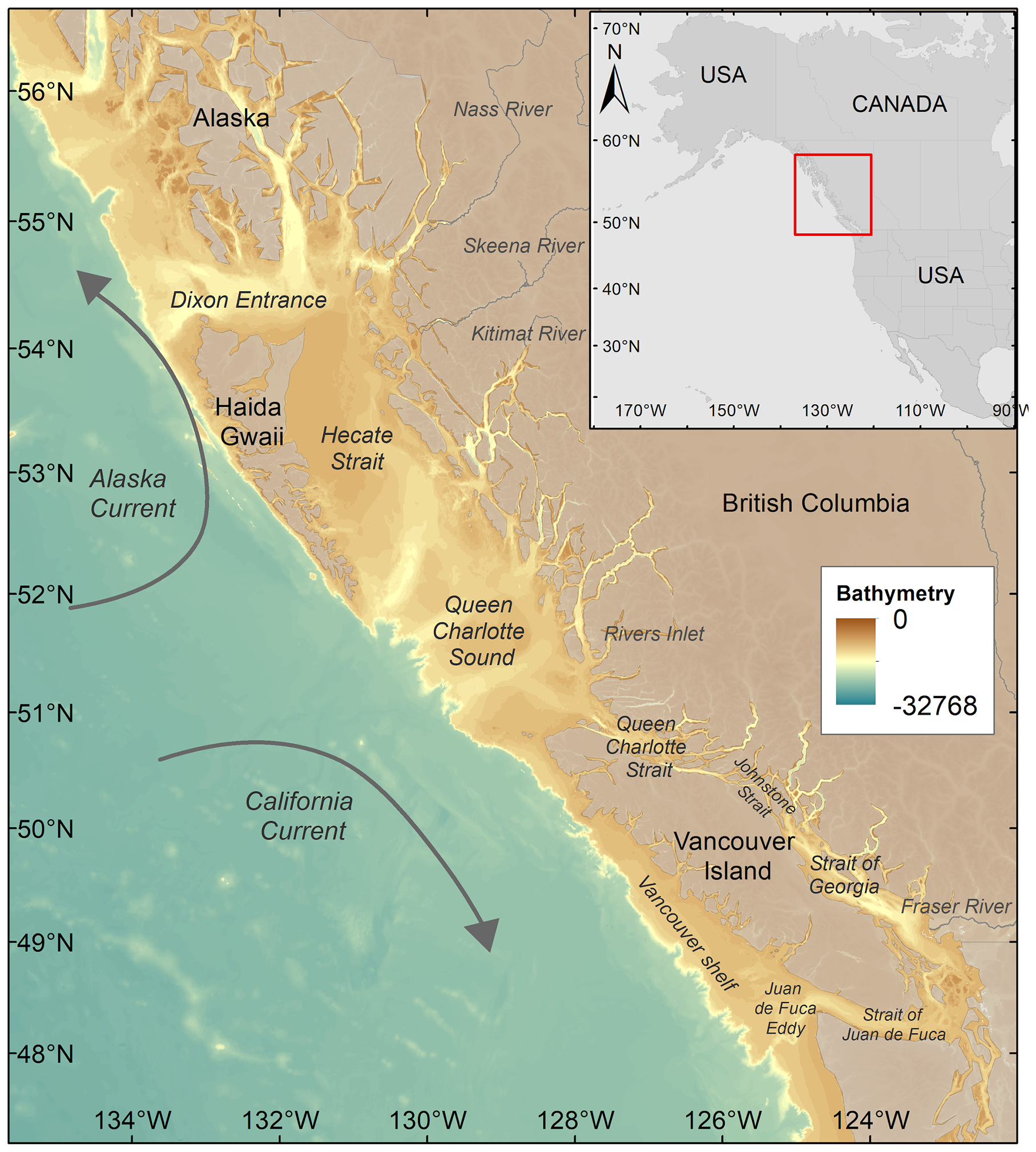
Study area map showing the two main currents (i.e., Alaska current and California current) and the bathymetry of the region. The names of the main rivers and locations cited in the text are also reported.
2.1 Satellite-derived time series of surface chlorophyll-a
The analysis was based on satellite-derived chlorophyll-a concentration from OLCI Sentinel-3A (ESA – European Space Agency) from April 2016 to December 2020. The Level-1 data were obtained from the EUMETSAT distribution through CODA (Copernicus Online Data Access). The Level-1 dataset was submitted to the atmospheric correction (AC; i.e., the process of removing the effects of the atmosphere on the reflectance values retrieved by satellite sensors.) using POLYMER processor (v 4.10), generating the Level-2 dataset. The recommended flags were applied on the daily products, i.e., ‘Cloud’, ‘L1 Invalid’, ‘Negative BB’, ‘Out-of-bounds’, ‘Exception’, ‘Thick Aerosol’, and ‘High Air Mass’ (Steinmetz et al., 2016) and the POLYMER “Case-2” flag was used to remove pixels where the chlorophyll-a estimates are known to be highly overestimated (Giannini et al., 2021). The “Case-2” flag indicates pixels where highly scattering turbid waters, occurring in coastal waters heavily influenced by terrestrial runoff during spring and summer (Phillips and Costa, 2017), generate poor reflectance retrievals, with substantial underestimation in the blue wavelengths, contributing to errors above 100% in chlorophyll-a (Giannini et al., 2021). Finally, the POLYMER Level-2 data were binned (note, the pixel-by-pixel median was preferred to the arithmetic mean to minimize the effect of possible outliers) into 8-day composites, generating the Level-3 dataset with 300 m spatial resolution for the entire study region. Overall, the POLYMER atmospheric correction algorithm can retrieve ocean color data under adverse conditions (i.e., high aerosol optical depths, high sun-glint, and thin clouds), providing a significantly improved coverage (Gittings et al., 2017). In addition, when applied to the Sentinel-3A data, the model provided the best performance when retrieving surface chlorophyll-a from Northeast Pacific coastal waters, outperforming other approaches, such as the C2RCC Neural Network (for further details, see the multi-metrics analysis in Giannini et al., 2021).
A workflow using the Microsoft Azure platform and Docker containers was developed to implement and optimize the data processing described above and create an automated tool for future analyses and monitoring programs (Figure 2). A total of ~8000 Level-1 daily scenes comprising the study area were downloaded in batch mode using a Python-based Sentinel satellite data downloader, developed by the Copernicus project for EUMETSAT, and stored in Blob Storage (i.e., a feature of Microsoft Azure that allows different types of data to be stored on the cloud) Level-1. The daily images were submitted to the AC using a pool of 100 nodes (working in parallel) in batch mode (Batch Pool AC; see Figure 2) executed in a specific POLYMER 4.10 Container. The atmospheric corrected chlorophyll-a Level-2 daily images were stored in the Blob Storage Level-2. Finally, the Level-3 Binning operation was executed in the SNAP application (v 7.0) implemented using a Docker container, using the 100 nodes of Batch Pool Binning (Figure 2). During the 8-day binning operation, the POLYMER quality flags were used, as recommended, to remove bad quality data (Steinmetz et al., 2016). The Level-3 weekly (8-day) data were then stored in the Blob Storage Level-3 and made available for further analysis (Figure 2).
Figure 2
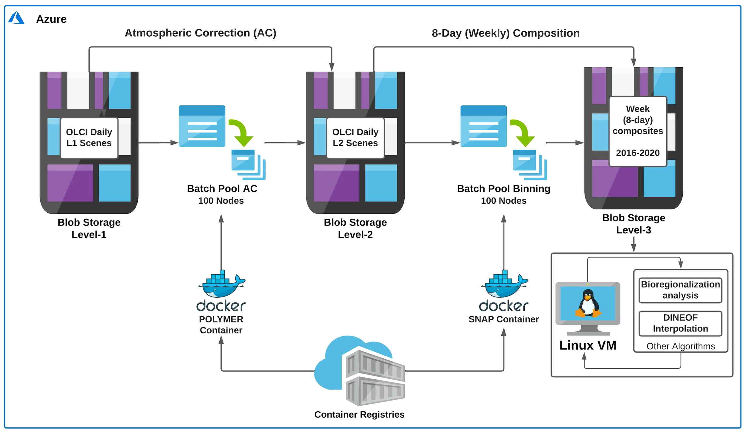
Workflow showing the main steps (i.e., atmospheric correction and binning) made on the Microsoft Azure cloud computing platform to obtain the Sentinel-3A Level-3 time series. The chlorophyll-a Level-1 dataset (~ 8000 scenes) was submitted to the atmospheric correction (AC) using POLYMER processor (v 4.10) to generate the Level-2 dataset. The latter was binned to create the 8-day chlorophyll-a Level-3 dataset with 300 m spatial resolution. All the tasks were made in parallel (i.e., using a pool of 100 CPU cores) and executed in specific containers. Finally, the DINEOF interpolation procedure and subsequent analyses were performed using a virtual machine within the Azure cloud platform. Note that the DINEOF output led to the generation of a cloud-free time series of 8-day composite chlorophyll-a images. For detailed information on the whole workflow, see section 2.1.
The above procedure resulted in a weekly (i.e., 8-day) composite time series with relatively high temporal resolution and limited missing data. Except for 2019, all years (i.e., 2016, 2017, 2018, and 2020) showed good spatiotemporal coverage (see Figure S1 in supplementary material). However, a Data Interpolating Empirical Orthogonal Functions (DINEOF) method (Beckers and Rixen, 2003) was applied to produce a gap-free chlorophyll-a time series. The DINEOF interpolation scheme (more details in supplementary material) has demonstrated effectiveness for filling spatial gaps in the remote sensing datasets (see Taylor et al., 2013) and was successfully applied to MODIS data for the Salish Sea on the south coast of British Columbia (Hilborn and Costa, 2018). This method allows a more accurate reconstruction of missing data without any a priori statistical information by identifying the dominant spatial and temporal patterns (Alvera-Azcárate et al., 2005). The 8-day gap-free time series (RMSE 0.16 mg/m3; 88.95% explained variance) was then used as input for the Self-Organizing Maps (SOMs) analysis (see next section). The interpolation procedure and all subsequent analyses were performed within the cloud platform using a virtual machine (Figure 2 – see small panel on the right).
2.2 Bioregionalization approach
The identification of bioregions across the coastal oceans of BC and SEA was based on a two-step classification procedure (Vesanto and Alhoniemi, 2000). First, we used a Self-Organizing Map (SOM) analysis to explore the spatiotemporal patterns of the input data (i.e., chlorophyll-a) and synthesize the most relevant features in a two-dimensional map. Subsequently, we used a clustering algorithm to reduce the number of units from the initial SOM partition into an objective number of clusters (i.e., bioregions). When the number of SOM units (or nodes) is significantly large, clustering the SOM units may facilitate the quantitative analysis of the map and data contained therein (Vesanto and Alhoniemi, 2000). A similar two-step classification procedure has been successfully used for partitioning different oceanic areas (e.g., Saraceno et al., 2006; Fendereski et al., 2014). Overall, the process leads to gathering regions that exhibit similarly shaped seasonal chlorophyll-a cycles. The procedure is schematically shown in Figure 3, while the primary two steps are discussed in the following subsections.
Figure 3
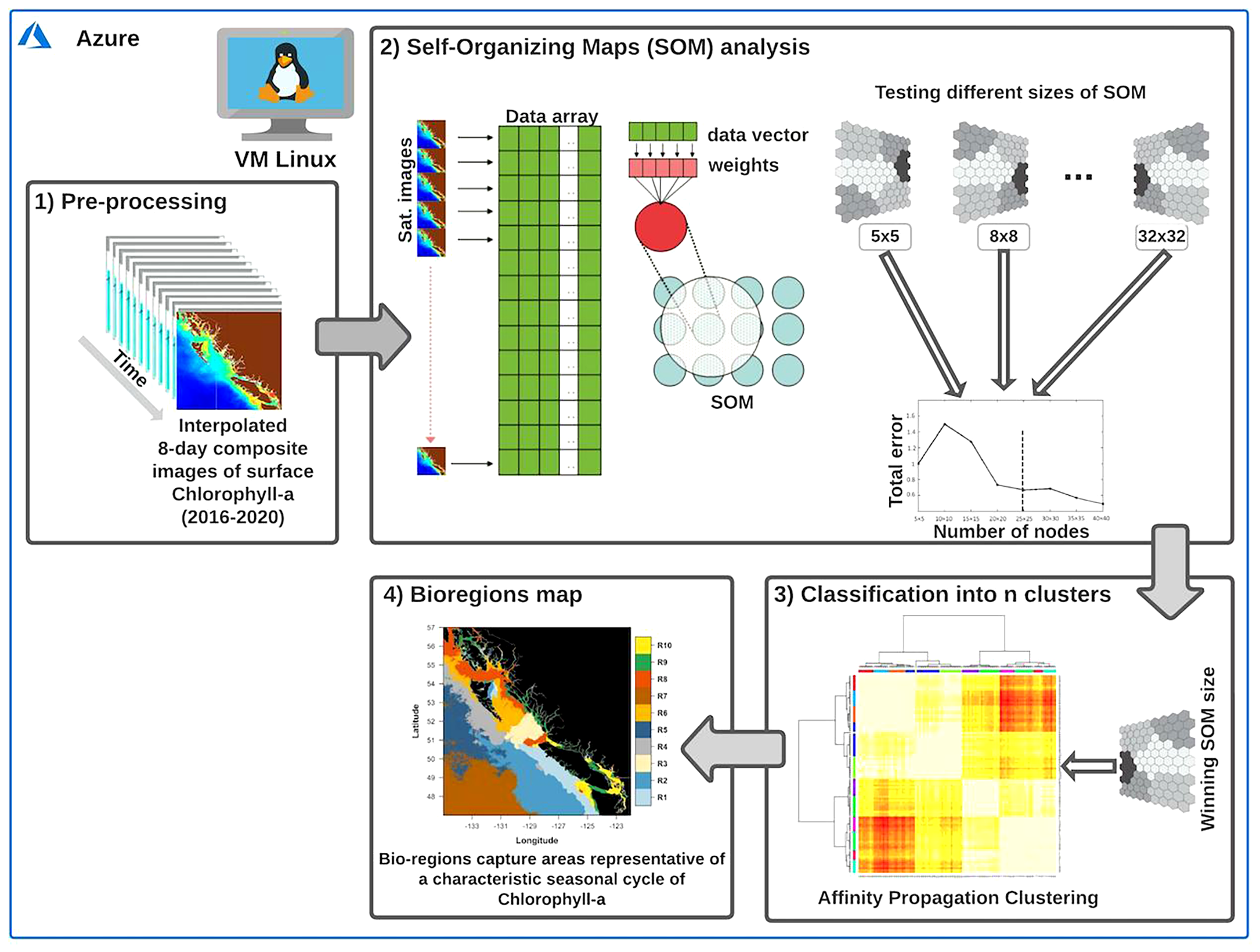
Outline of the two-step classification procedure performed on the Azure virtual machine to obtain the bioregions. The interpolated 8-day composite images of chlorophyll-a (box 1) represent the primary input for the Self-Organizing Map (SOM) analysis (box 2). As a second step, an Affinity Propagation clustering algorithm (box 3) was used to reduce the number of units (i.e., nodes) from the initial SOM partition into an objective number of clusters (box 4). For more detailed information on the two-step classification procedure, sees section 2.2. Modified from Liu and Weisberg (2011) and Fendereski et al. (2014).
2.2.1 Self-organizing maps analysis
The SOMs analysis (Figure 3 - Box 2) was developed by Teuvo Kohonen (Kohonen, 1982) and is a robust unsupervised neural network algorithm (i.e., no need for a priori, empirical, or theoretical description of the input-output relationships) designed to reduce large and high dimensional datasets to a 2D network of nodes (or units). SOM has been used for various applications in meteorology and oceanography fields (see Liu and Weisberg, 2011 for a review). More details on the SOM training algorithm, evaluation of its performance, and examples of applications in oceanography are provided by Richardson et al. (2003). One of the main characteristics of the SOM is the preservation of the topological relationships of the input data i.e., similar nodes are mapped close together on the neural network, facilitating pattern recognition in large and complex satellite datasets (Richardson et al., 2003). In other words, at the end of the learning process, while different patterns are located further apart, those similar are arranged to be neighboring units on the neural network.
The SOM analysis (Figure 3 - Box 2) was carried out using the R package “Kohonen” ver. 3.0.10 (Wehrens and Kruisselbrink, 2018). Before performing the SOM analysis, the chlorophyll-a time series (Figure 3- Box 1) was log-transformed, and an 8-day climatology was created by averaging the log10-transformed chlorophyll-a values. The rationale for using the log-transformed climatology as a learning database was two-fold: 1) to minimize the effect of very high chlorophyll-a values (especially in coastal areas) and to better consider the full range of variability, ranging from the lowest offshore chlorophyll-a values to the highest coastal ones, and 2) to capture the dominant seasonal cycle shapes of chlorophyll-a. To ensure differentiation of seasonal cycles of similar shape but with a different amplitude, the 8-day climatology was arranged into a matrix composed of pixel-normalized values. Specifically, the seasonal cycle was normalized at each pixel by the annual mean as in Foukal and Thomas (2014) and Huot et al. (2019). Since we were specifically interested in the temporal variability, we addressed the SOM analysis in the time domain (Liu et al., 2016). Consequently, input data vectors (i.e., observations) have been built using the climatological time-series at each grid point (i.e., pixel). Thereby, the SOM pools input data into subsets of similar chlorophyll-a temporal patterns, and all observations in a subset are thus assigned to a node.
Concerning the SOM’s grid parametrization, nodes (or units) were arranged on a hexagonal grid as it favors neither the horizontal nor the vertical direction. At the same time, a lower topographic error (i.e., a projection quality indicator) was ensured by using the Gaussian neighborhood function (Fendereski et al., 2014). Finally, the batch algorithm was selected to train the SOM, and the Euclidean distance was used to determine the similarity between nodes during the training phase. The latter requires selecting an optimal number of nodes (note that the number of nodes defines the dimension of the matrix and, thus, the size of the SOM – for example, 3x3 nodes give a map’s size of 9) and iterations (i.e., number of steps – at each step of the batch training process, all observations - input vectors - are presented to the SOM nodes before updating their values). Although no theoretical principle exists, the choice of the map size is of fundamental importance since it may affect the results (Richardson et al., 2003). As such, following Elizondo et al. (2021), a rough estimate of the optimal map size (M) was based on the total number of data points (i.e., pixels) in the dataset and computed with the following formula:
where w is the number of weeks, and ni s the number of data points in the dataset. Using equation (1), we obtained a value of M approaching a SOM of size ~32 x 32. Therefore, keeping the SOM dimension of 32 x 32 as a reference point, we trained SOMs of different dimensions (between 5 x 5 and 50 x 50) and compared them to another according to their total error changes (see Figure S2 in supplementary material). The total error, as in Fendereski et al. (2014), was defined as the sum of the topographic error (TE) and quantization error (QE). The optimal SOM size was thus based on a threshold criterion. Specifically, the first map size chosen had the least number of nodes, after which changes in total error did not decrease appreciably (> 5%) when more nodes were added (Fendereski et al., 2014; Elizondo et al., 2021). In our case, the cutoff criterion identified the dimension of 29 x 29 as the optimal SOM dimension (see also Figure S3 for a sample density plot for SOM map quality). Interestingly, the 29 x 29 SOM expressed more than 85% of the variance and was close to the map size (i.e., 32 x 32) suggested by equation (1). Regarding the number of iterations used to train the SOM, the batch-training algorithm converges significantly faster, and 350 steps were sufficient to converge the training processes toward a plateau. Additional tests showed that changes to different combinations of training parameters (e.g., the use of another distance metric or an increased number of steps) did not reduce the total error. However, by maintaining the same training parameter combinations, different learning procedure replications may yield slightly different node partitions. This is due to the initialization of the node’s weight vector and the order in which the data is thus presented (Solidoro et al., 2007). To minimize this effect, node weights were initialized using a PCA-based method, and the entire procedure was repeated twenty times. The resulting 29 x 29 SOMs were finally compared using the Fowlkes-Mallows (FM) similarity index (Fowlkes and Mallows, 1983). The comparison led to calculating a matrix of FM similarity indexes from which the SOM having the highest FM value was chosen and used for the next step.
2.2.2 Classification into n clusters (bioregions)
Clustering similar nodes can summarize the qualitative information provided by the SOM. We used the Affinity propagation (AP) clustering algorithm (Frey and Dueck, 2007 - see Figure 3 – Box3). Unlike other clustering algorithms (i.e., as K-means), AP does not require one to specify a priori the number of clusters. The AP algorithm is based on a “message passing” scheme in which items (i.e., data points) compete to become exemplars. Therefore, the algorithm identifies exemplars among data points and forms clusters of data points around these exemplars. The latter are data points that are the best representative of themselves and some other data points. The algorithm, simultaneously, considers all data points as potential exemplars and exchanges messages between them until a specific set of exemplars and corresponding clusters emerge. In other words, a cluster only has one exemplar (i.e., a cluster center), and all points associated with the same exemplar are placed in the same cluster (Frey and Dueck, 2007).
As an input, the algorithm requires information on 1) similarity and 2) preference. Similarity reflects how well-suited a data point is to be another one’s exemplar. The negative Euclidean distance, the default option in Frey and Dueck (2007), was used to measure similarity between pairs of data points. The number of identified exemplars (number of clusters) emerges from the message-passing procedure, but the values of the input preference also influence it. Specifically, low preference values lead to small numbers of exemplars, while high preference values lead to many exemplars. By default, the preference value is initialized to the median (q = 0.5) similarity value between all input pairs, resulting in a moderate number of clusters (Frey and Dueck, 2007). To be conservative (i.e., obtaining the lowest number of clusters), we set this value to the minimum (q = 0). The AP clustering algorithm on the previously chosen SOM of size 29 x 29 (see the previous subsection) led to the identification of ten clusters. The analysis was carried out using the R package “APCluster” ver. 1.4.8 (Bodenhofer et al., 2011).
Finally, to test whether bioregions differed in their biological characteristics (i.e., annual mean, maximum, timing of maximum, etc.), a non-parametric, one-way analysis of variance by ranks (Kruskal–Wallis H test) was performed (Fendereski et al., 2014; Ardyna et al., 2017). The biological characteristics were calculated from the 8-day climatology time series for each pixel within the same bioregion using standard R functions (i.e., mean, max, min). A significant result (p< 0.05) of the Kruskal-Wallis H test implies that at least one bioregion differs from all others. Moreover, a multi-step a posteriori pairwise testing procedure (i.e., Dunn’s test) was applied to identify which bioregions differ significantly from the others (Fendereski et al., 2014).
2.3 Timing of the spring bloom onset
The onset of the spring bloom can be a reasonably accurate indicator of the productivity of specific marine fish populations. For example, Malick et al. (2015) reported a statistically significant correlation between spring bloom timing and pink salmon productivity in Alaska and British Columbia populations. Different metrics are typically used to define the onset of spring bloom with remotely sensed data. These metrics may, for example, identify the time in which chlorophyll-a concentrations first reach a predefined absolute concentration (e.g., Jackson et al., 2015), and define the time when the maximum growth rate is attained (e.g., Marchese et al., 2019; Mayot et al., 2020), or when chlorophyll-a concentrations first rise above a threshold criterion (e.g., Zhai et al., 2011; Marchese et al., 2017; Suchy et al., 2022), with latter being the most widely used. The threshold criterion can be estimated from the remotely sensed chlorophyll-a time series by fitting a Gaussian function to the time series or carrying out a cumulative sum (CUSUM) of the chlorophyll-a concentration (see Racault et al., 2015, and the references therein). Given that our 8-day chlorophyll-a time series is well distributed in time (i.e., with no missing data), and to account for the full range of chlorophyll-a variability (i.e., ranging from the lowest off-shelf values to the highest on the coastal shelf), the start day of the spring bloom was estimated using the CUSUM method along with the utilization of a threshold criterion. More precisely, the time at which the cumulative biomass curve at each pixel reaches 15% of the total biomass was identified as the bloom initiation (Brody et al., 2013). The choice of the 15% threshold was based on tests done using other threshold percentages (i.e., 5%, 10%, and 20%) and comparing the results to each other (data not shown). Excluding the 5%, the different thresholds provided similar results, with 15% yielding estimates closer to those obtained in previous studies. Overall, the used method prevented the use of multiple absolute concentrations (e.g., Jackson et al., 2015); at the same time, it defined the bloom start date even when the chlorophyll-a increase was not distinctly noticeable (i.e., low seasonal variation), and its inherently smoothing nature helped to reduce short chlorophyll-a pulses and thus potential “noise” in the data (Chiba et al., 2012; Ferreira et al., 2014; Racault et al., 2015).
3 Results
This section is organized as follows: first, we present the chlorophyll-a monthly climatology estimated from five years (2016-2020) of Sentinel 3-A observations. Second, we introduce the ten bioregions obtained from the two-stage procedure and chlorophyll-a’s corresponding seasonal climatological cycles. Finally, we present the spring bloom onset results in the context of the bioregions.
3.1 Monthly climatology of chlorophyll-a
Monthly climatology estimated from five years (2016-2020) of Sentinel 3-A observations provided a comprehensive synoptic view of the seasonal chlorophyll-a variability over the area of interest (see Figure 4). High chlorophyll-a concentrations were found throughout the platform, where some productivity hotspots are most noticeable. For instance, regions of high chlorophyll-a concentration were observed in the Strait of Georgia (SoG) in the proximity of the Fraser River, along the Vancouver Island shelf, in Queen Charlotte Strait, north of Vancouver Island, and further north in the area surroundings Dixon Shelf and Hecate Strait. Moderate levels of phytoplankton biomass were found along the continental slope, while low mean chlorophyll-a concentrations, on the other hand, were observed in offshore waters. The monthly climatological cycle showed chlorophyll-a concentrations in February at ~0.3 mg/m3 in offshore waters and, generally, close to ~1 mg/m3 over the shelf. In March, an increase in chlorophyll-a concentrations (~1.3 mg/m3) was noticeable in the southern part of our study area (i.e., in the Strait of Georgia and Vancouver Island shelf). Further north, a similar increase in chlorophyll-a concentrations was visible on the east coast of Haida Gwaii. In April and May, chlorophyll-a concentrations were visibly enhanced across the continental shelf and remained relatively high in summer (i.e., from June to August), especially around Vancouver Island waters. Spring blooms were less noticeable in offshore waters (i.e., beyond the shelf-break), where chlorophyll-a concentrations were low (~0.3 mg/m3) and quasi-constant through the summer. In offshore waters, an increase in chlorophyll-a concentrations (~0.9 mg/m3) was visible only later in the fall (i.e., from September to mid-November). By mid-November, chlorophyll-a values were reasonably low throughout the area of interest, except for some strictly coastal areas where values were still relatively high. From late November through January, low incident sun angle and persistent cloud cover prevented examination of satellite-derived chlorophyll-a data.
Figure 4
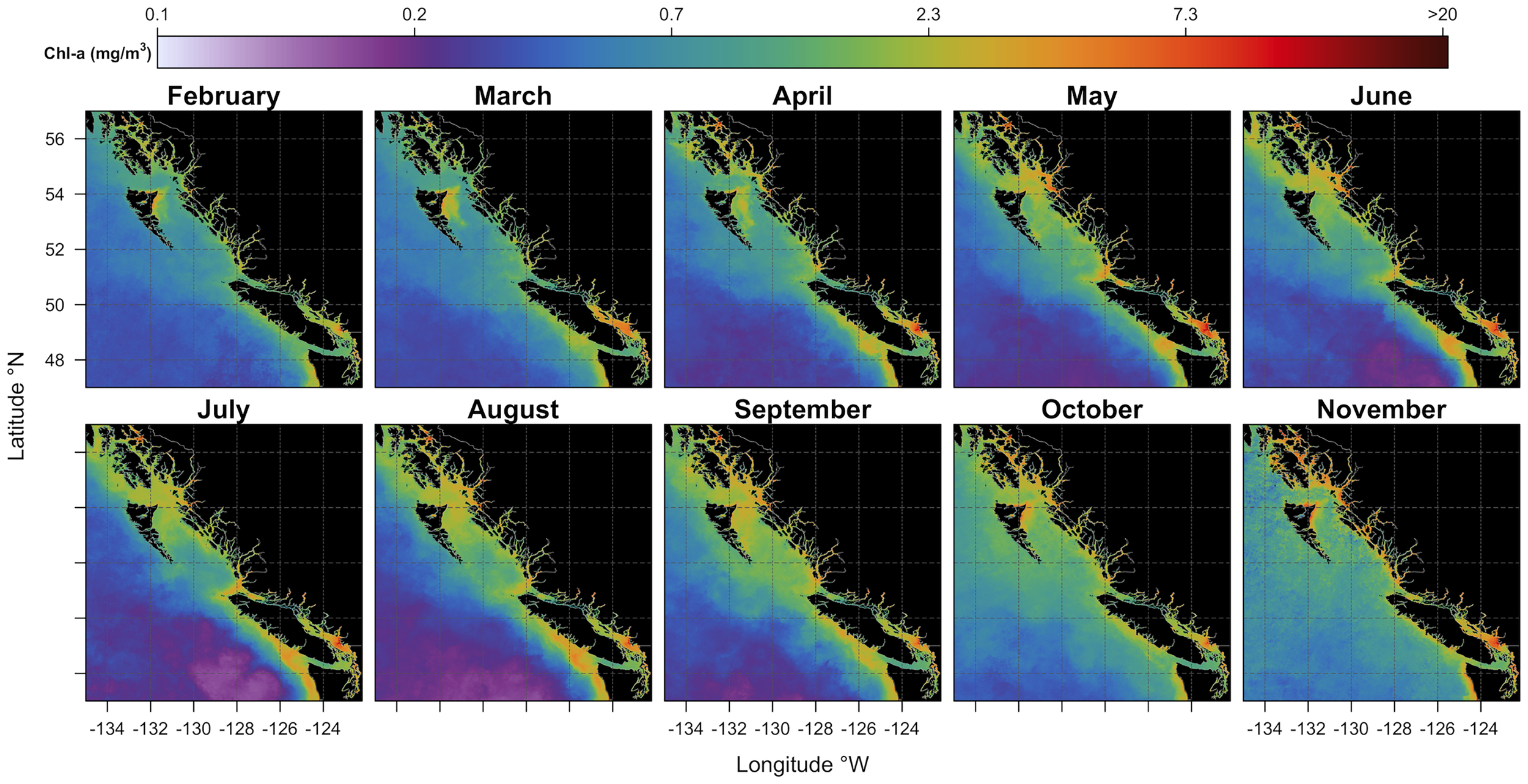
Monthly climatological (mean 2016-2020) maps of chlorophyll-a concentration expressed in mg/m3 (see the colored bar on the top). Black areas denote the land.
3.2 Bioregions and climatological seasonal cycles
The ten bioregions obtained from the two-step procedure and the climatological seasonal cycle of chlorophyll-a for each bioregion are shown in Figures 5 and 6, respectively. Bioregions were grouped into two broad classes, using the shelf break position (i.e., the 1000 m isobaths) as a discriminating criterion, defining the separation between off-shelf (i.e., #2, 4, 5, 7; Figure 6A) and neritic (i.e., #1, 3, 6, 8, 9, 10; Figure 6B) bioregions. The bioregions area coverage is shown in Figure S4 (supplementary material).
Figure 5
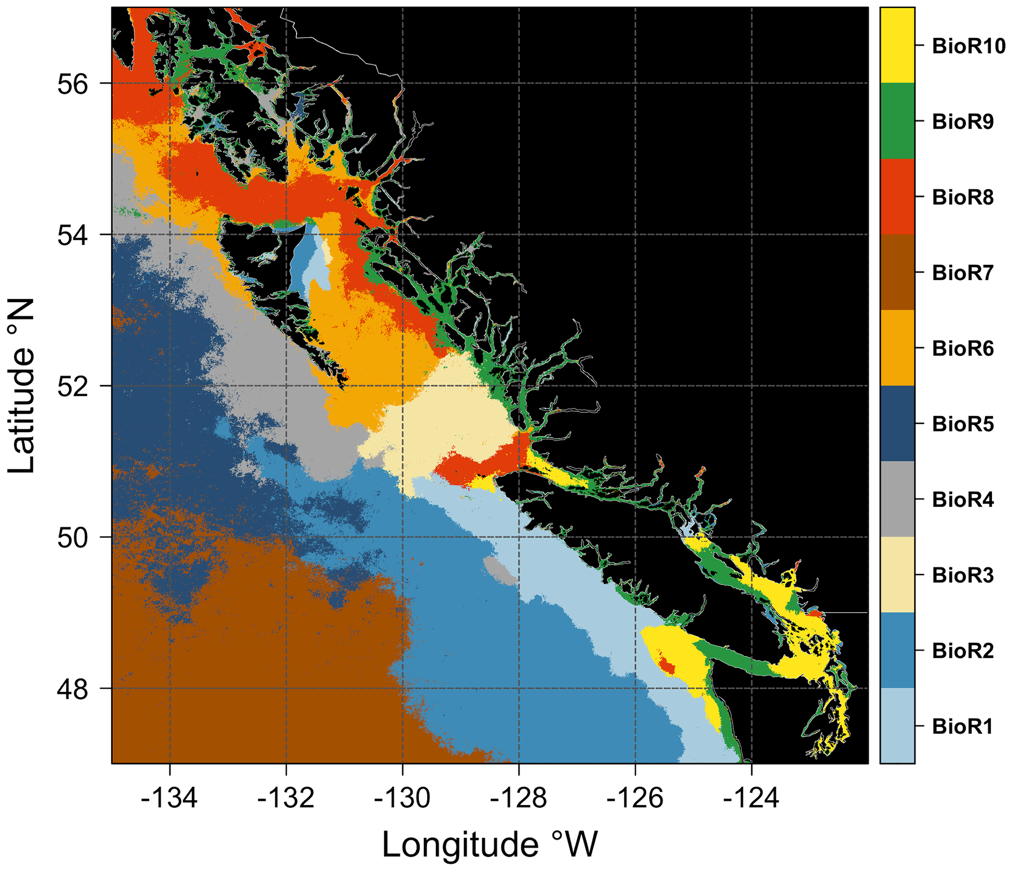
Maps showing the spatial distribution of the ten bioregions obtained from the two-step classification procedure (see Figure 3). Each bioregion is assigned a color (see the vertical bar on the left). Black areas denote the land.
Figure 6
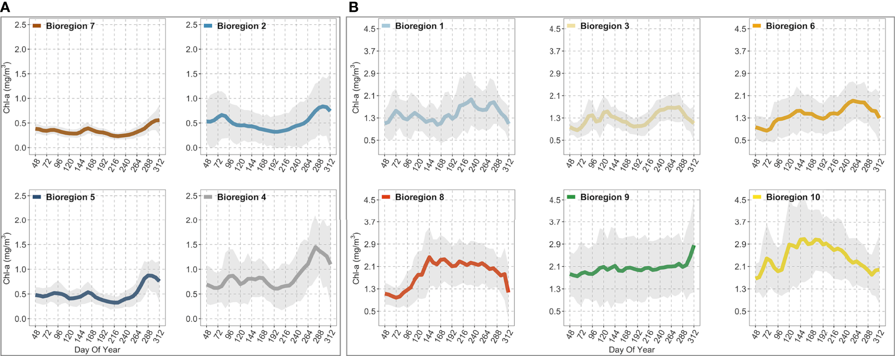
Figure showing the climatological seasonal cycles of chlorophyll-a (thicker colored lines) for each bioregion. (A) contains the four (i.e., #2, 4, 5, 7) off-shelf/shelf-break bioregions. (B) contains the six (i.e., #1, 3, 6, 8, 9, 10) neritic bioregions. The shaded areas represent the standard deviation (± SD). The seasonal cycles were obtained from 8-day composites of Sentinel-3 data over 5 years (2016-2020) spatially averaged over bioregions shown in Figure 5. The day of the year (DOY) is reported on the x-axis, while chlorophyll-a concentrations (mg/m3) are reported on the y-axis on different scales, depending on the box. Note that each color corresponds to that used in Figure 5 and identifies the same bioregion.
Off-shelf, the two outermost bioregions, i.e., #5 and #7, displayed the lowest chlorophyll-a concentrations during spring (i.e., peaks were below ~0.5 mg/m3 ± 0.32; Figure 6A). Later in mid-October, chlorophyll-a increased steadily to a maximum of about ~0.87 mg/m3 ± 0.26 in bioregion #5, but it remained lower (0.59 mg/m3 ± 0.31) in bioregion #7. Overall, both bioregions were characterized by weak seasonality, with chlorophyll-a remaining very low throughout the year with concentrations that, on average, were below 1.00 mg/m3. The seasonal chlorophyll-a cycles of the other two off-shelf bioregions, #2 and #4 (Figure 6A), although featuring slightly higher chlorophyll-a values than bioregions #5 and #7, were still characterized by a marked lack of spring bloom with concentrations below than 1.00 mg/m3. Specifically, bioregion #2 was characterized by a mean seasonal cycle of chlorophyll-a showing a peak around mid-March (~0.65 mg/m3 ± 0.48) and a second, more pronounced (~0.87 mg/m3 ± 0.6), in late October (Figure 6A). On the other hand, in bioregion #4, the spring bloom peaked slightly later in early April (~0.86 mg/m3 ± 0.54), while an autumn maximum (~1.48 mg/m3 ± 0.65) was reached around mid-October (Figure 6A). Compared to bioregion #2, the fall chlorophyll-a maximum was higher in bioregion #4 and occurred slightly earlier (see Figure 7E). Finally, among the off-shelf bioregions, the climatological seasonal cycle of bioregion #4 was characterized by higher chlorophyll-a concentrations (Figure 6 but see also Figures 7A–D).
Figure 7
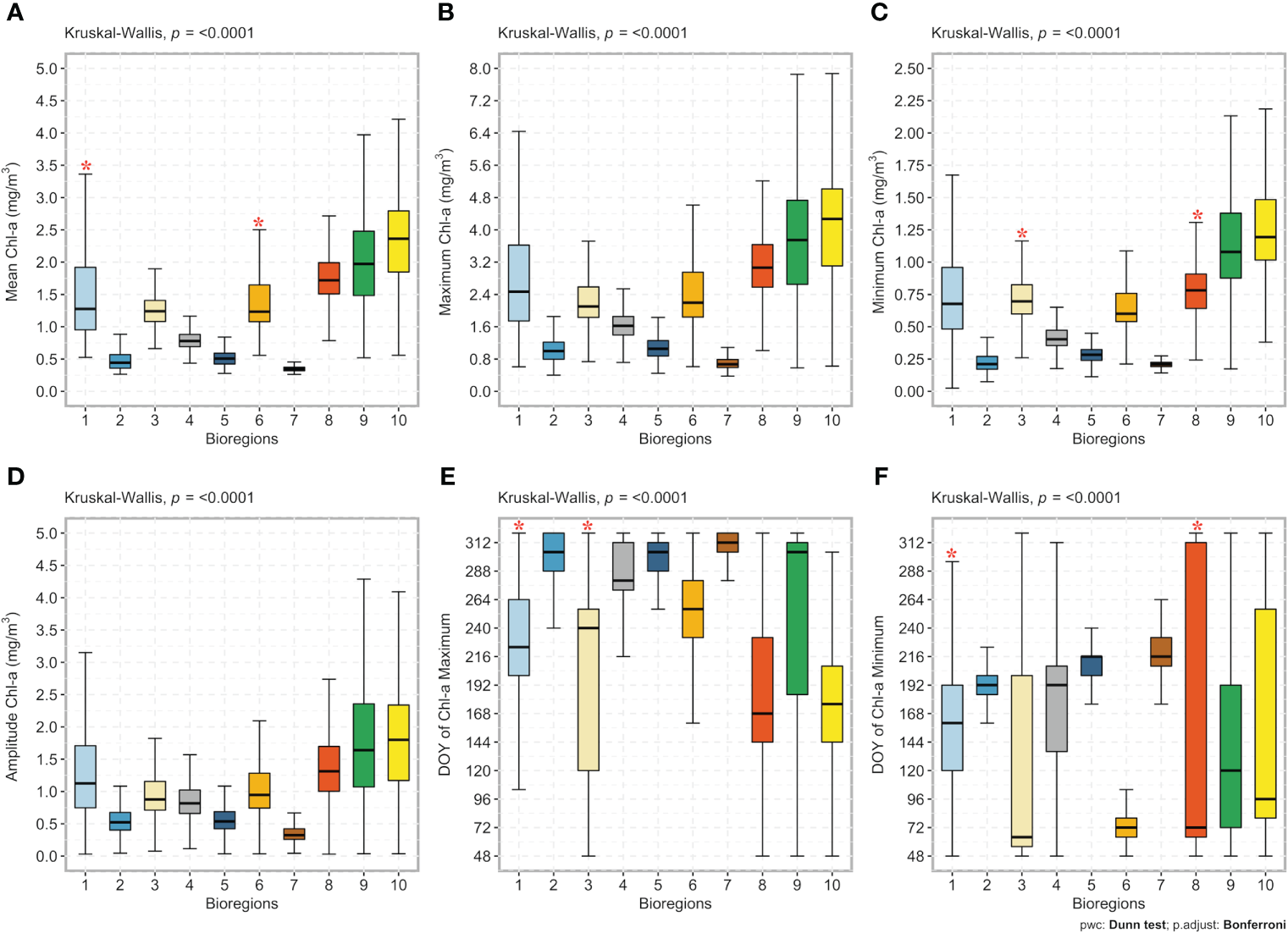
Box plots of the bioregions (1 to 10; x-axis) against (A) the annual mean chlorophyll-a concentration (mg/m3), (B) the annual chlorophyll-a maximum (mg/m3), (C) the annual chlorophyll-a minimum (mg/m3), (D) the annual amplitude (i.e., the difference between the annual maximum and the annual average; mg/m3), (E) the timing of the bloom maximum (day of the year - DOY), and (F) the timing of the bloom minimum (DOY; y-axis). The line in the middle of each box represents the median. The top and bottom limits of each box are the 25th and 75th percentiles, respectively. The lines extending above and below each box (i.e., whiskers) represent the full range of non-outlier observations for each variable beyond the quartile range. The Kruskal-Wallis H test results are shown on the top of each figure (A–E). A significant result (p < 0.05) of the Kruskal-Wallis H test implies that at least one bioregion differs from all others. The results of Dunn’s multiple comparison test are also shown. Red asterisks * depict bioregions (x-axis) without statistically significant differences between the climatological input variables (y-axis), whereas no asterisks depict significant differences at the 95% level (p < 0.05) between bioregions. Note that each box color corresponds to that used in Figure 5 and identifies the same bioregion.
Neritic bioregions (i.e., those along the continental shelf area) were, on average, marked by higher chlorophyll-a concentrations and more pronounced seasonal cycles (Figure 6B). Overall, bioregions #1, #3, and #6 were characterized by bimodal chlorophyll-a seasonal cycles (i.e., two annual peaks). In contrast, bioregions #8 and #10 were described by a single peak-bloom and thus exhibited different seasonal characteristics. Finally, bioregion #9 was marked by the absence of a clear seasonal cycle, displaying a gradual but slow increase in biomass with higher values reached in the fall (~2.86 mg/m3 ± 1.68). Specifically, bioregion #1 was characterized by two main maxima, the first in early March (~1.56 mg/m3 ± 0.78) and the second in late August-early September (~1.96 mg/m3 ± 0.92), after which values remained high until mid-October before beginning to decline (Figure 6B). Bioregion #3 exhibited a noticeable spring bloom that peaked in late April or early May (~1.53 mg/m3 ± 0.6), while the fall maximum, of similar amplitude (~1.66 mg/m3 ± 0.46), was reached in late September mid-October (Figure 6B). As with the seasonal cycles of bioregions #1 and #3, bioregion #6 follows similar behavior. In the latter, spring bloom peaked in late May (~1.56 mg/m3 ± 0.7) and reached an autumn maximum (~1.92 mg/m3 ± 0.7) in the second half of September, after which chlorophyll-a values dropped in October and November. In bioregion #8, the spring peak (~2.43 mg/m3 ± 1.05) was reached in late May, but it was not until late September that chlorophyll-a concentrations gradually decreased (Figure 6B). Finally, bioregion #10 showed a similar seasonal cycle shape to bioregion #8; however, the spring peak was reached between March (i.e., when a first peak was noticeable at ~2.3 mg/m3 ± 0.93) and May (~3.05 mg/m3 ± 1.51), while from July to November, chlorophyll-a values progressively decreased (Figure 6B).
The Kruskal-Wallis H test revealed the statistical differences of the six seasonal cycle characteristics (i.e., annual mean, maxima, minima, amplitude, and the timing of the bloom maximum and minimum), which were supported by the multi-step a posteriori pairwise (Dunn’s test) comparisons (Figure 7). Results showed significant differences in the annual mean chlorophyll-a concentration among all bioregions, except for bioregions #1 and #6 (Figure 7A). Significant differences were also found for the yearly chlorophyll-a maximum among all bioregions (Figure 7B) and annual amplitude (Figure 7D), and excluding bioregions #3 and #8, results also showed significant differences in the annual minimum (Figure 7C). Finally, except for bioregions #1 and #3 for the onset of the bloom maximum (Figure 7E) and bioregions #1 and #8 for the beginning of the bloom minimum (Figure 7F), the timing of minima and maxima differed significantly among the remaining bioregions. Except for a few cases, significant differences between bioregions were detected for all six seasonal cycle characteristics. Boxplots also showed that the highest chlorophyll-a concentrations were observed in bioregions #10 and, more broadly, in bioregions located on the continental shelf (i.e., neritic bioregions). Conversely, bioregions in the deep basin (i.e., #5 and 7) appeared to be the least productive. Further, in some bioregions, the annual maximum is reached in autumn, as highlighted in Figure 7.
3.3 Timing of the phytoplankton spring bloom
The mean time of the seasonal increase (i.e., the onset of the spring boom) in chlorophyll-a (estimated from the climatological average time series of chlorophyll-a in each pixel) is shown in Figure 8A. The seasonal increase in chlorophyll-a occurred, on average, earlier south of ~51°N of latitude. However, the study area also noticed localized zones characterized by earlier (later) phytoplankton blooms. South of ~51°N, the timing of the seasonal increase in chlorophyll-a generally happened from late February to late March (i.e., between days 64 and 88 of the year - Figure 8A). Specifically, locally distinct zones of earlier start dates were visible in the open ocean, in Juan de Fuca Strait, and in the northern part of the Strait of Georgia. Late blooms happened around the Juan de Fuca eddy region, the north tip of Vancouver Island, and in Queen Charlotte Strait. In Queen Charlotte Sound, between Vancouver Island and Haida Gwaii, the increased chlorophyll-a concentrations occurred between mid and late March (Figure 8A). Along the coast, north of ~52°N, the bloom started late on the west coast of Haida Gwaii, in Hecate Strait, and along Dixon Entrance, with dates ranging from the beginning of April to the beginning of May (i.e., between days 96 and 120 of the year - Figure 8A). Finally, a large area of earlier start dates (i.e., in March) was evident along the north end of the east coast of Haida Gwaii, around Dogfish Banks (Figure 8A).
Figure 8
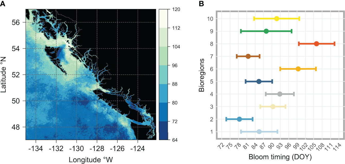
Figure showing (A) the climatological (2016-2020) spring bloom onset dates across the whole area of interest, and (B) for each bioregion (i.e., obtained averaging all pixels that are within each cluster). The vertical color bar in (A) indicates the day of the year (DOY), with colors ranging from dark blue (early bloom) to white (late bloom). In (B), the colored dots (each color corresponds to that used in Figure 5 and identifies the same bioregion) represent the mean, and the horizontal bars represent the standard deviation (± SD).
The latitudinal gradient in the bloom onset timing noted earlier (Figure 8A) was, to some extent, also noticeable at the bioregion level, with the average start date differing appreciably (Figure 8B; see also Table S1). South of~51°N, the spring bloom started earlier in bioregions #1 (DOY 85.43 ± 7.52) and #2 (DOY 78.35 ± 4.71), covering Vancouver Island shelf and the adjacent open ocean area. Also, bioregion #7, which occupies the offshore waters south of 51°N, was characterized by a relatively early (DOY 81.5 ± 4.09) spring bloom. Moving northward (roughly between 51°N and 53°N), the spring bloom started later in bioregions #3 (DOY 90.32 ± 4.5), #4 (DOY 92.82 ± 5.03), and #5 (DOY 85.33 ± 4.76). On the shelf, the spring bloom started even later in the two bioregions further north, #6 and #8, respectively DOY 99.38 ± 6.43 for bioregion #6 and DOY 106.03 ± 6.4 for bioregion #8. Lastly, the spring phytoplankton bloom began in late March (DOY 87.96 ± 9.07) for bioregion #9, which encompasses a wide latitudinal gradient and covers very coastal areas, most deep fjords, and inlet regions, and at the end of March/beginning of April (DOY 91.7 ± 8.09) for bioregion #10, occupying most of the Strait of Georgia and other peripheral areas.
Beyond the observed spatial trends in bloom timing, interannual variability and consistent spatial patterns are also noticeable, as shown in Figures 9 and 10. For instance, the area of earlier start dates along the north end of the east coast of Haida Gwaii appears to be a recurring pattern. On an interannual basis, the latitudinal gradient previously observed in the bloom start climatology (Figure 8A) was less evident, and more significant differences were apparent for 2019 and 2020. In 2019, the spring bloom began earlier in a large area south of ~51°N (Figure 9C). In contrast, in 2020, a noticeable delay in the spring bloom timing was observable in offshore waters (i.e., above 130°W) and along the entire latitudinal gradient (Figure 9D). These interannual differences were reflected, to some extent, across the bioregions (Figure 10). For example, in 2019, seven of the ten bioregions (i.e., #1, 2, 3, 4, 5, 6, 9) showed an earlier spring bloom, while for the year 2020, four of the ten bioregions (i.e., #4, 5, 6, 7) showed a later spring bloom (Figure 10). Interestingly, results also showed that although the initiation of the spring bloom onset may differ from year to year for the same bioregion (Figure 10), the range of temporal variability in bloom onset among the ten bioregions was very similar to that observed in climatology (Figure 8B, e.g., bioregions #1 and #2 have the earliest blooms, whereas bioregion #8 has late blooms).
Figure 9
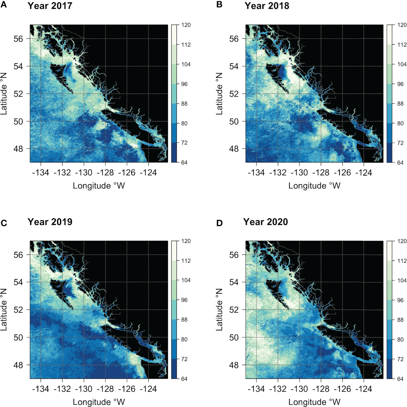
Maps showing the spring bloom onset dates across the study area for the years (A) 2017, (B) 2018, (C) 2019, and (D) 2020. The vertical color bar indicates the day of the year (DOY), with colors ranging from dark blue (early bloom) to white (late bloom).
Figure 10
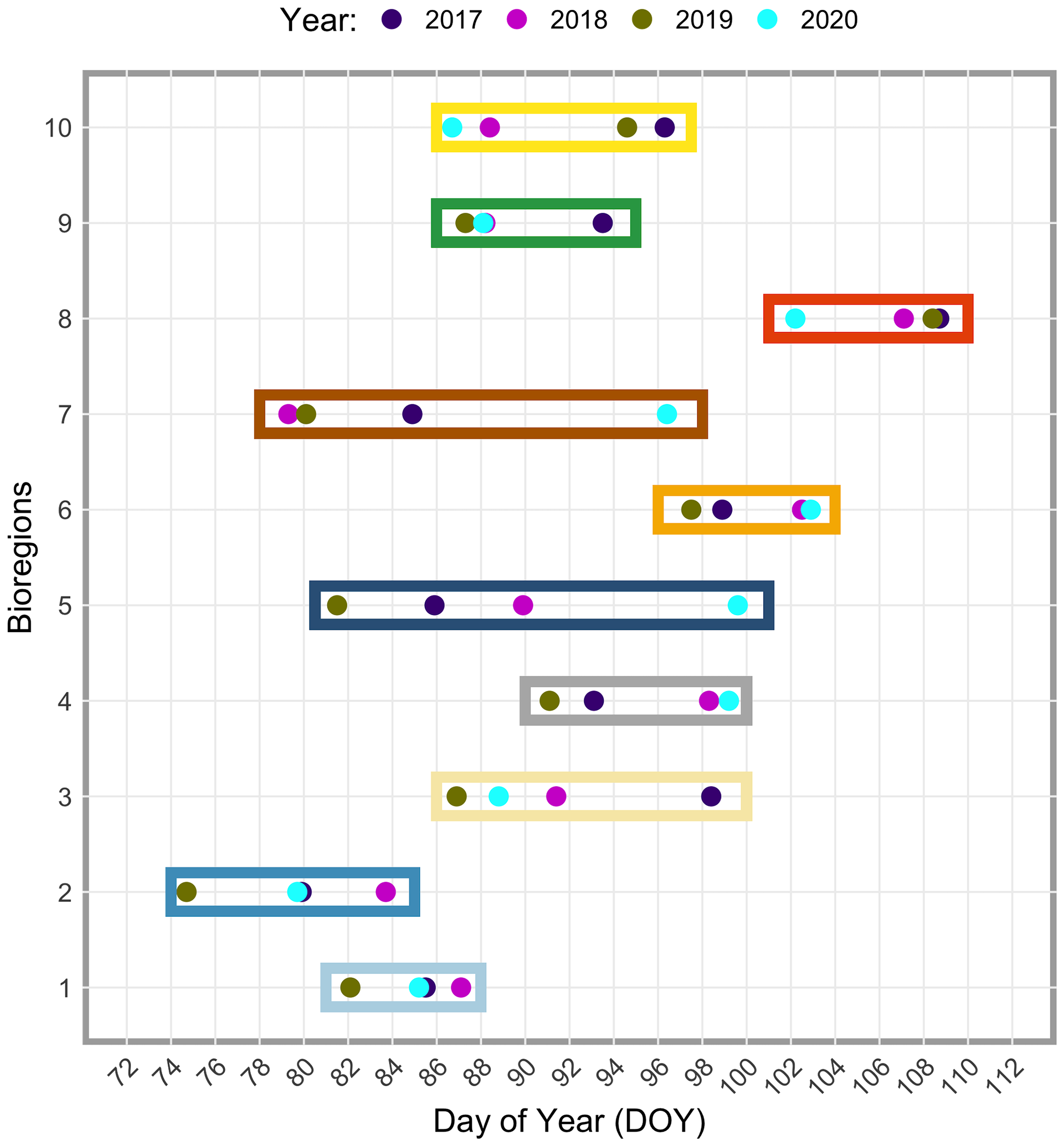
Inter-annual (2017-2020) differences in spring bloom onset date among the ten bioregions. Different years are indicated with different colored dots (see the top of the figure). The colored dots are grouped within a box corresponding to a specific bioregion (y-axis). Note that each color used for the boxes corresponds to that used in Figure 5 and identifies the same bioregion. The day of the year (DOY) is reported on the x-axis. See also Table S1 in the supplementary material.
4 Discussion
This study used objective analysis of Sentinel-3A data to identify ten bioregions in the coastal to offshore ocean waters of BC and SEA. The geographic location of the bioregions was partly coupled to the spatial distribution of chlorophyll-a concentrations (Figure 4). Oligotrophic bioregions, showing low mean values of chlorophyll-a concentrations, matched precisely with clusters #2, 4, 5, and 7. Bioregions #2 and #4, located immediately west of the continental shelf-break, defined a transition zone that marks the boundary between the more productive bioregions (i.e., #1, 3, 6, 8, 9, 10) on the continental shelf and the more oligotrophic deep basin (i.e., west of ~128°W). This onshore-offshore gradient is consistent with prior satellite studies in this region (Brickley and Thomas, 2004; Jackson et al., 2015; Giannini et al., 2021) and a recent regional coupled circulation-ecosystem model (Peña et al., 2019a). The ten bioregions identified by the two-step classification over the research domain were separated based on their chlorophyll-a seasonal cycle. Below we discuss the identified bioregion characteristics in detail, while Table 1 summarizes the main features of the off-shelf/shelf-break and neritic bioregions.
Table 1
| Bioregions | Main covered area | Main characteristics | |
|---|---|---|---|
|
Off-shelf bioregions
(i.e., oceanic area) |
Bioregion #7 | Offshore south | Bioregions beyond the shelf-break margin Characterized, on average, by low chlorophyll-a concentrations (< 1 mg/m3) Spring blooms slightly pronounced – onset between mid-March and early April Mixed Layer Depth (MLD) shoaling triggers the spring bloom initiation More prominent fall blooms (compared to spring blooms) Iron limitation restrains phytoplankton growth in spring and early summer Phytoplankton biomass accumulates in late summer/fall (reduced zooplankton grazing) |
| Bioregion #5 | Offshore north | ||
| Bioregion #4 | Northern shelf-break |
||
| Bioregion #2 | Southern Shelf-break |
||
|
Neritic bioregions
(i.e., continental shelf area) |
Bioregion #1 | Vancouver shelf | Bioregions located on the continental shelf Characterized by high chlorophyll-a concentrations (>> 1 mg/m3) Phytoplankton assemblage is usually dominated by large phytoplankton cells Presence of unimodal (one-peak) and bimodal (two-peaks) seasonal cycles Spring blooms onset, on average, between the end of March and the beginning of May The availability of nitrate may limit productivity Zooplankton grazing may also disrupt or delay phytoplankton blooms Upwelling, tidal mixing, and freshwater input shape phytoplankton blooms dynamic Basin-scale variations may also influence phytoplankton dynamics on the shelf |
| Bioregion #3 | Central BC shelf | ||
| Bioregion #6 | Northern shelf | ||
| Bioregion #8 | Inner northern shelf |
||
| Bioregion #9 | Inner coastal waters and fjord |
||
| Bioregion #10 | Strait of Georgia and Juan de Fuca Eddy |
Main characteristics of neritic and off-shelf bioregions.
Note that each color corresponds to that used in Figure 5 and identifies the same bioregion.
4.1 Off-shelf and shelf-break bioregions
Off-shelf bioregions (i.e., #5 and #7) together with the two bioregions of the transition zone (i.e., #2 and #4) occupied an area extending from the continental shelf-break (~1000 m) to the deep basin (> 3000 m). Interestingly, these bioregions intersect approximately at the point where the Subarctic Current splits (i.e., between 45°N – 50°N and 130°W – 150°W) into the clockwise flowing California Current and the anticlockwise flowing Alaska Current (see Figure 1). Relatively low values of biomass distinguished off-shelf bioregions, which also displayed autumn peaks that were generally more prominent than spring peaks. Low temporal variability in upper-layer chlorophyll-a concentrations has been previously reported at Ocean Station Papa (OSP; 50°N, 145°W) and along the offshore section of the Line P (Peña et al., 2019a). Similar to our findings, Yoo et al. (2008) reported that in the eastern subarctic Pacific, between ~40°N and ~55°N, the annual chlorophyll-a maximum occurs in the autumn. These findings were also confirmed by a later satellite-based study by Zhang et al. (2017) that revealed a seasonal pattern with a small peak in spring and chlorophyll-a reaching its maximum in fall/winter. Recently Zhang et al. (2021a), using observations from a biogeochemical-Argo float (BGC-Argo), showed that the seasonal variability in surface (~7 m) chlorophyll-a for this region was consistent with satellite observations: phytoplankton biomass begins to increase in late summer, reaching a distinct peak at the end of September before decreasing in late October and November. These bioregions occurred thus in waters characterized by iron-poor and nitrate-rich conditions (Martin et al., 1991; Boyd et al., 2004; Nishioka et al., 2021). Iron supply governs bloom dynamics in high-nitrate, low-chlorophyll (HNLC) areas, and Fe limitation prevents the occurrence of diatom blooms (i.e., large phytoplankton cells), which are frequent on the shelf (Ribalet et al., 2010), thus explaining the lack of marked spring phytoplankton blooms. The efficient grazing of micro-zooplankton can also impact spring phytoplankton blooms, and mesozooplankton consumption of micro-zooplankton may be an essential factor in the phytoplankton biomass accumulation that starts in late summer and peaks in autumn (Zhang et al., 2021a). Occasionally, higher abundances of diatoms are observed offshore, probably fostered by episodic supplies of Fe (Boyd and Harrison, 1999). Off-shelf bioregions may also receive iron from the atmosphere via dust (Martin et al., 1989) and the continental margin through strong tidal currents or the formation of westward-propagating eddies (Cullen et al., 2009). For instance, the region off the coast of the Haida Gwaai (~51°N, 134°W) is a marine area where anticyclonic mesoscale Haida eddies commonly form in the winter and early spring and move slowly westward, transporting nutrients and high iron coastal water offshore (Harrison et al., 2004; Crawford et al., 2005). Eddy formation could partially explain the slightly higher chlorophyll-a values (i.e., when compared to other off-shelf bioregions) in bioregion #5 and particularly in bioregion #4, which lie on the typical trajectory of these eddies. In contrast, the lower chlorophyll-a values in bioregions #2 and #7 were likely due to the influence of the California Current, which has a lower nutrient concentration than the Alaska current (Whitney et al., 2005), the tendency for shelf primary productivity to be entrained into the shelf-break current rather than exported to the open ocean, and the lack of eddy influence in these regions (Peña et al., 2019a). Overall, the shelf break/slope area (i.e., bioregions #2 and #4) defines a transition zone between iron-rich, nitrate-poor shelf waters to iron-poor, nitrate-rich offshore waters (Peña and Varela, 2007; Ribalet et al., 2010).
4.2 Neritic bioregions
The neritic bioregions (#1, 3, 6, 8, 9, and 10) were more productive than off-shelf bioregions and had a different seasonal cycle (see Figures 6 and 7 but also Figure S5 in supplementary material). Bioregion #1, covering the Vancouver Island shelf, had two chlorophyll-a peaks, the first in March-April and the second in mid-October, similar to satellite-based observations by Sackmann et al. (2004). Similarly, Jackson et al. (2015) associated the waters encompassing the south and the west of Vancouver Island with a seasonal cycle featuring a March-April peak and a higher intensity fall peak. Geographically, this same bioregion can be associated with the so-called “green” cluster found by Foukal and Thomas (2014), characterized by a seasonal cycle with a spring peak in April-May and a long, late summer elevated period from July through October. Therefore, this area appears to have long-term consistency in bloom dynamics. Overall, blooms dynamic in bioregion #1 generally follows wind-driven upwelling events that resupply nutrients into the euphotic zone through vertical advection (Sackmann et al., 2004; Foukal and Thomas, 2014; Cyr and Larouche, 2015; Jackson et al., 2015).
Bioregions #3 and #6 mainly covered the area of Queen Charlotte Sound and Hecate Strait (see Figure 1) and are described as a highly productive and iron-rich marine region (Whitney et al., 2005; Cullen et al., 2009; Jackson et al., 2015). Oceanographic conditions across these bioregions are determined primarily by winds, coastal runoff, and light levels (Whitney et al., 2005). Prevailing southeast winds force strong downwelling in winter, while a transition to northwest winds in April leads to cessation or weakening of downwelling, and the productive season starts. During the summer (June-August), the absence of strong winds and freshwater runoff promote stratification. Conditions change at the end of summer with winds increasing in strength and, by the end of October, deteriorate rapidly with the onset of storm activity (Thomson, 1981; Whitney et al., 2005). Not surprisingly, therefore, these bioregions showed a bimodal pattern in chlorophyll-a concentrations, with a spring peak in April-May and a second peak in September. Similar bimodal seasonal cycles were observed by Jackson et al. (2015) in Southern Alaska, Hecate Strait, and Queen Charlotte Sound and therefore associated under a single chlorophyll-a wide-shelf regime. Similarly, Waite and Mueter (2013), using model-based cluster analysis, identified, among other regions in the Gulf of Alaska (GOA), a coast-wide “eastern GOA” cluster characterized by relatively intense spring and fall blooms occurring in May and September. While bioregions #3 and # 6 shared a bimodal seasonal pattern, they had relevantly different seasonal cycles. These differences that can be seen in the slopes of the seasonal cycle curve and the summer minima highlight this area’s spatial complexity. Moreover, our analysis also identified bioregion #8, which in contrast to the previous regions (i.e., bioregions #3 and #6), was marked by a seasonal cycle with a single peak bloom at the end of May. This bioregion covered a narrow area on the inner shelf that stretched from the south to the north through Dixon Entrance. In inner shelf environments, prolonged production during the summer may be due to the sustained input of nutrients into the surface layer, possibly due to a continually mixed and re-stratified water column (Henson, 2007; O’Neel et al., 2015; Stabeno et al., 2016). Furthermore, bioregion #8 also included the area of Cook Bank, south of Queen Charlotte Sound and close to the northern tip of Vancouver Island, which receives well-mixed and nutrient-rich waters from Queen Charlotte Strait (Borstad et al., 2011; Tortell et al., 2012).
Bioregion #9, which included the Fraser River mouth, inner coast waters, and most of the complex fjord systems across the study area, was the only bioregion that did not show a clear seasonal cycle. We speculate that this was likely due to runoff-driven estuarine circulation resupplying nutrients which keeps chlorophyll-a concentrations relatively high and stable under an adequate light regime. Interestingly, the straits of Johnstone and Juan de Fuca were also included within bioregion #9. Well-mixed waters characterize both areas due to persistently weak stratification, high nutrients, and light-limited production with no clear blooms (Masson and Peña, 2009; McKinnell et al., 2014; Dosser et al., 2021; Mahara et al., 2021).
Finally, bioregion #10 covered most of the Strait of Georgia and the Juan de Fuca Eddy area (48.5°N, i.e., north of Washington and south of Vancouver Island). This bioregion had a spring peak, and chlorophyll-a concentration remained high through the summer. Previous studies of phytoplankton production in the SoG have shown that light conditions, river runoff, tides, wind, and complex nutrient and grazing dynamics shape its spatial and inter-annual variability (Yin et al., 1997; Li et al., 2000; Masson and Peña, 2009; Suchy et al., 2019). However, despite slight differences between northern, central, and southern SoG, average annual primary production and phytoplankton biomass cycles increase in spring and maintain relatively high summer primary production, a feature particularly evident in the central and south portion of the SoG, as evidenced by Peña et al. (2016) employing a coupled three-dimensional biophysical model. Recently, Suchy et al. (2019) also reported a lack of a bimodal pattern in the chlorophyll-a climatology in the central and northern SoG regions. The Juan de Fuca eddy area supports elevated nutrient concentrations that promote high phytoplankton biomass to the eddy margins (Hickey and Banas, 2008; MacFadyen et al., 2008). Using a model to simulate generalized plankton production, including diatoms, copepods, and euphausiids, Robinson et al. (1993) showed increased diatom biomass from a winter minimum to a spring maximum that remained relatively high throughout the summer before declining later in September from growth limitation by nutrients, light availability, and high zooplankton grazing. The phytoplankton bloom dynamic described above is consistent with the seasonal cycle observed for bioregion #10, although the latter also includes the SoG.
4.3 Variability in spring bloom timing
The dynamic of the bloom onset timing is of great ecological importance due to the interconnected effects between food webs and fisheries (Platt et al., 2003; Platt et al., 2007; Suchy et al., 2022). The method used in this paper to retrieve the spring bloom start dates across the BC and SEA coastal oceans provided results that reasonably agreed with previous estimates determined by other methods. Specifically, a latitudinal gradient with earlier blooms south of ~51°N latitude was observable in the climatology (Figure 8). However, results also showed spatial heterogeneity in bloom timing, which can be illustrated by analyzing and contextualizing the differences among the ten bioregions.
There was a minimal seasonal change in phytoplankton productivity in offshore waters, covered by bioregions #2, 4, 5, and 7. Our results showed that spring bloom initiation dates varied, on average, from early March to the beginning of April. Sasaoka et al. (2011) reported that chlorophyll‐a concentrations for an equivalent offshore region (i.e., group C - eastern North Pacific) were, on average, consistently low (< 1 mg/m3) and that the mean spring onset date of mid-March had considerable variability (DOY 77 ± 50). These authors speculated that the El Niño phase (warmer SST) and La Niña phase (cooler SST) might modulate water column stability (stratification) and thus blooms dynamic. For example, the cooler phase could induce vigorous mixing and an efficient supply of nutrients that would affect the peak bloom duration (Sasaoka et al., 2011). In situ measurements at the Ocean Station Papa (OSP; 50°N-145°W) showed that surface waters can be mixed down to ~120 m deep during the winter (Harrison, 2002). During winter, deep mixing leads to low light availability within the mixed layer. Only later in spring, as incident irradiance increases and the Mixed Layer Depth (MLD) decreases, do chlorophyll-a concentrations increase, and a nitrate drawdown begins in April (Harrison, 2002). In offshore waters, the contribution of tidal mixing and freshwater input is approximately equal to zero, and the MLD shoaling appears to be the main factor triggering the bloom initiation (Henson, 2007; Cole et al., 2015). However, Fe limitation can still restrict phytoplankton growth (Zhang et al., 2021b; Zhang et al., 2021a). Lam et al. (2006) showed that iron replenishment from the continental shelves could allow early (even as early as February) phytoplankton blooms in offshore waters given adequate light levels. Phytoplankton growth might therefore be enhanced by an increase in either irradiance or iron (Peña et al., 2019b). Further, mesoscale eddies may enhance nutrient transport, the spatiotemporal variance in the phytoplankton biomass and control the timing of spring phytoplankton blooms (Doney et al., 2003; Whitney et al., 2005; Maúre et al., 2017; Glover et al., 2018). Hence, across off-shelf bioregions, differences in bloom initiation dates could be due to changes in water column stability and mesoscale variability (e.g., eddies), which may drive shifts in phytoplankton bloom dynamics from a few days to weeks.
Overall, on the shelf, oceanographic features, such as freshwater runoff, upwelling, and tidal mixing, can cause notable shifts in bloom initiation times over short distances (Daly and Smith, 1993; Henson, 2007). Specifically, the northern continental shelf (i.e., north of ~51°N) was covered by bioregions #3, #6, and #8. Until March, large portions of this broad area are well mixed due to tidal mixing, and waters only start to stratify in mid-April (Henson, 2007). Similar to Jackson et al. (2015), the average spring bloom start date for bioregions #6 and #8 was mid-April. However, in bioregion #3, which was located slightly further south (i.e., central BC coast), the spring bloom start date fluctuated between March and April. North of ~51°N, both tidal and wind-driven mixing may modulate primary production pulses (Henson, 2007; Peña et al., 2019a). Hence, the balance between mixing (i.e., tide and wind) and buoyancy (i.e., heat and freshwater) processes appears to be crucial in triggering the bloom onset across these bioregions (Henson, 2007; O’Neel et al., 2015).
Moving further south, in bioregion #1 (Vancouver Island shelf), the spring bloom generally started at the end of March. This result is consistent with the average start month (i.e., March) of spring bloom indicated by Jackson et al. (2015) and mid-March to late April identified by Henson and Thomas (2008) for approximately the same region. Over this bioregion, the variability in the bloom onset is likely related to the timing of the beginning of upwelling-favorable winds (Henson and Thomas, 2008; Foukal and Thomas, 2014). Light seems to limit phytoplankton growth more strongly than nutrients on the Vancouver Island shelf (Peña et al., 2019a). As such, although episodes of favorable-upwelling winds may occur as early as February, the net daily light experienced by phytoplankton is still insufficient to support its growth (Henson and Thomas, 2008).
Finally, in our bioregionalization, the SoG was represented by bioregions #9 and #10, which, on average, were defined by spring bloom timing at the end of March. This is consistent with defined spring timing for this region based on different methods and temporal scales. For instance, Schweigert et al. (2013); Jackson et al. (2015), and Suchy et al. (2022), based on satellite chlorophyll-a estimates, found March as the dominant time of spring bloom initiation. Further, our results were consistent with the long-term (1968 to 2010) mean spring bloom start date in the Central SoG of March 25 found by Allen and Wolfe (2013) using a one-dimensional biophysical model. Peña et al. (2016), using a coupled three-dimensional biophysical model, observed that while the bloom peak is attained during the first two weeks of April, phytoplankton biomass typically starts to increase in February, and higher concentrations are reached in March, which is also consistent with our findings for bloom initiation. Given the dynamical differences in environmental conditions for phytoplankton growth in the SOG, the debate over which physical forcing most influences the spring bloom timing in SoG is still open. Indeed, while some authors (Collins et al., 2009; Allen and Wolfe, 2013) found that the spring bloom is controlled primarily by wind and that freshwater input has an insignificant effect on the timing of the bloom, other authors (Peña et al., 2016) indicate that, on average, the growth of phytoplankton starts when solar radiation increases, possibly before significant shoaling of the mixed layer and the development of stable stratification. Zooplankton grazing may also disrupt or delay phytoplankton blooms (Suchy et al., 2022).
The latitudinal gradient in bloom timing was less pronounced on an interannual basis (Figure 9). However, depending on the year, the recurrence of specific spatial patterns was still observable. For example, the area of earlier start dates along the north end of the east coast of Haida Gwaii is a recurrent pattern. Results also showed that the bloom starts slightly earlier each year in the northern part of the SoG. This feature was most likely associated with weaker winds and tidal currents, leading to calm conditions and increased stratification that characterize the north SoG (Peña et al., 2016; Del Bel Belluz et al., 2021). However, it has also been suggested that inlets could play a role in seeding the early bloom in the strait (Gower et al., 2013). Early spring blooms in Sechelt Inlet and Malaspina Strait appear to be a recurrent feature (e.g., 2005, 2008, 2009; Gower et al., 2013), which could fuel the main spring bloom in the SoG (Gower et al., 2013). Results also showed a marked difference in spring bloom timing between 2019 and 2020 (Figure 9). Winter oceanographic conditions in 2019 and 2020 differed in surface temperature (on average, the region during 2020 was cooler than in 2019), eddies formation, and circulation patterns (Pakhomov et al., 2022). To some extent, these interannual differences were captured by the identified bioregions (Figure 10). Compared to 2020, in 2019, large portions of the region displayed early seasonal increases in chlorophyll-a, with seven of the ten bioregions showing an earlier spring bloom. Albeit strongly influenced by localized dynamics, interannual differences in phytoplankton growth may also be correlated with fluctuations in large-scale climate indices (e.g., Pacific Decadal Oscillation [PDO], North Pacific Gyre Oscillation [NPGO], North Pacific Index [NPI]) and thus to basin-scale variations (Henson, 2007; Di Lorenzo et al., 2008; Peña et al., 2019a; Suchy et al., 2019). For instance, Suchy et al. (2022) recently found that spring bloom initiation in the SoG correlated with both SOI (positive correlation) and PDO (negative correlation): with warmer years leading to earlier and more intense spring blooms and colder years exhibiting average or late blooms.
5 Data and method caveats
Several caveats should be considered when interpreting our results. The approach’s constraints are primarily related to the inherent errors in the ocean color data. For instance, a considerable burden on our region is usually associated with cloud coverage. Although using a higher resolution (i.e., 300 m in our case) shows an improved cloud-free probability (Feng et al., 2017), daily images displayed a coverage, with few exceptions, below ~50% (data not shown). Reducing time resolution from daily to weekly (8-days) partially overcame this problem. Except for 2019, the percentage of valid data coverage in the 8-day composites time series ranged from 40% to over 90% (see Figure S1 in supplementary material), facilitating the interpolation. We recognize that daily temporal resolution may help resolve fine-scale ocean processes and more closely monitor the annual cycle of phytoplankton biomass. However, the 8-day composites time series represents an optimal compromise to reduce the computation times without renouncing a good spatiotemporal coverage (Cole et al., 2012). For instance, 8-day composite chlorophyll-a concentration images have been successfully used to characterize the biogeographical conditions of other oceanic areas (e.g., D’Ortenzio and Ribera d’Alcalà, 2009).
Satellite-derived chlorophyll-a estimates can also be affected by inorganic sediment and colored dissolved organic matter (CDOM) entering the BC and SEA coastal oceans via freshwater discharge (Carswell et al., 2017; Giannini et al., 2021). The high-turbidity waters in the study region are typically limited to a narrow band along the coast and in the proximity of river plumes. To minimize the influence of suspended sediments and CDOM, we followed the quality procedures suggested by Giannini et al. (2021). For instance, the POLYMER ‘Case-2’ pixels were removed, thus reducing the possible bias associated with turbid coastal waters and providing chlorophyll-a Sentinel-3A retrievals within expected ranges for the Northeast Pacific coastal waters (Giannini et al., 2021). It is also worth restating that although some degree of error might still be associated with the retrieved chlorophyll-a values (Giannini et al., 2021), the regionalization approach used in this work emphasizes differences in the shapes of the seasonal cycles rather than in the absolute values of the chlorophyll-a concentrations (Foukal and Thomas, 2014; Mayot et al., 2016; Ardyna et al., 2017). As such, we believe that the spatiotemporal patterns observed in this work were not significantly affected by either sediment or CDOM.
In our analysis, we assumed that similar (different) seasonality of surface chlorophyll-a reflected similar (different) mechanisms governing the functioning of the pelagic ecosystem. However, we recognize that with the present dataset (i.e., the use of satellite-derive surface chlorophyll-a data), it was impossible to account for subsurface patterns of phytoplankton biomass. A comparison of satellite data and in situ bottled chlorophyll-a samples conducted by Suchy et al. (2019) across the Strait of Georgia indicated that high chlorophyll-a concentrations, when present below the surface (e.g., 10 or 20 m), were also reflected in satellite surface measurements. Notwithstanding, discrepancies between surface and subsurface patterns could still arise, mainly when a deep-water chlorophyll-a maximum occurs (Suchy et al., 2019). A certain degree of error may also be associated with spring bloom start dates. This could be due to several factors (e.g., data gaps, different algorithms or models to retrieve chlorophyll data) and different methods and metrics (Ferreira et al., 2014). Although the technique employed in this study allowed us to obtain spring bloom onset dates that reasonably agreed with previous estimates from other studies, we recognize that the method used may have missed the primary bloom onset in some cases, for example, across the off-shelf bioregions where fall blooms were, on average, more prominent than spring peaks. The importance and impacts of both spring and fall bloom characteristics on the food web should be considered with more attention in future studies by employing a specific algorithm to retrieve metrics and map phytoplankton phenological changes. Nevertheless, the method employed to retrieve the bloom onset dates combined with the 300 m spatial resolution of the Sentinel-3A highlighted differences among bioregions while giving, for the first time, a high-resolution and large-scale picture of the spring phytoplankton bloom onset.
Finally, another concern/limitation is associated with the time series length (2016-2020). The extent to which this 5-year coverage may account for longer-term chlorophyll-a variability is unknown. A significantly longer time series (>20 years) would have allowed us, for example, to discriminate periods based on anomalies of critical environmental variables (e.g., Sea Surface Temperature – SST) or specific climate indices (e.g., NPGO). Such discrimination would have led to climatologies being useful for retrieving time-resolved bioregions under different environmental conditions. However, as the first step, the climatological bioregionalization performed in this study identified specific regions reflecting the dominant seasonal cycle shapes, thus laying the foundations for future and target ecosystem investigations.
6 Conclusion and outlook
Several biogeographic marine classifications have emerged in the past decades, considering different approaches and associated spatial scales and scopes (e.g., fisheries, environment, and conservation management). Within this context, on a global scale, our area of interest intersects, for example, with three broad provinces (i.e., Eastern Pacific subarctic gyres [PSAE], Alaska coastal downwelling [ALSK], and Coastal Californian current [CALC] – more details in Longhurst, 2010) or two large near-surface marine ecosystems (i.e., offshore northern Pacific and coastal areas – see Zhao et al., 2020), depending on the biogeographic classification considered. Our partitioning provided a higher level of spatial details and, as such, did not correspond with those obtained from global biogeographic classifications. This is normal as these global biogeographic classification systems provide a broad perspective, and their representation of Northeast Pacific coastal and shelf seas do not capture the dynamics of the coastal oceans of BC and SEA, which are geomorphologically and oceanographically complex (e.g., shallow and deep waters, straits, fjords). The complex marine ecosystems of Canada’s Pacific have also been partitioned at a regional scale into four major marine biogeographic units through a national science advisory process that considered oceanographic processes and bathymetric similarities (DFO, 2009). However, a critical factor in implementing a biogeographic framework based primarily on empirical evidence (i.e., datasets analysis and expert opinions) is the difficulty of incorporating new data and new insights as they arise. As a result, it may take time to redefine these units spatially by scaling them down (or up) into smaller (or larger) units that are still ecologically meaningful. For instance, in our bioregionalization, the large DFO Offshore Pacific biogeographic unit has been objectively subdivided into four bioregions (#2, 4, 5, 7). In addition, the datasets employed may lack completeness (i.e., data gaps) and consistency due to sampling in different seasons and years. In this regard, our goal was to provide a regional biogeochemical partitioning that minimizes subjectivity and can be refined and continuously updated as more Sentinel-3 data becomes available to address future bioregions change due to different environmental conditions.
Overall, this study was built on previous works that used remotely sensed chlorophyll-a data to achieve bioregionalization based on the analysis of phytoplankton biomass patterns (e.g., D’Ortenzio and Ribera d’Alcalà, 2009). To the best of our knowledge, this is the first bioregionalization of oceanic regions across the coastal oceans of BC and SEA using highly resolved chlorophyll-a satellite data and an objective classification approach. In particular, the ten bioregion-dependent phytoplankton seasonal cycles were consistent with recognized oceanographic conditions in the study area and thus valuable for deciphering their complexity and highly dynamic nature. The latter was emphasized by the spring bloom timing that differed markedly among bioregions and inter-annually due to different environmental conditions. Bioregions have been shown to capture spatiotemporal variability in bloom onset dates, making the differences displayed very compact and objective.
By highlighting the crucial role of physical forcing in regulating phytoplankton dynamics in a very narrow latitudinal range, the findings of this study strengthen the view that the coastal oceans of BC and SEA cannot be considered homogeneous entities. Therefore, the current research results support biotic data-based regionalization as a framework to improve our knowledge of phytoplankton dynamics and thus promote future comparative analyses among bottom-up versus top-down controls within the coastal oceans of BC and SEA. Looking to the future, when more high-resolution data are available, the application of the method, as expressed above, should consider variability (stability) in the spatial distribution of bioregions. Indeed, objectively defining the latter with satellite data can help dynamically identify changes in bioregion boundaries. Tracking such changes can be potentially helpful and vital for the phenological analysis of phytoplankton and zooplankton, which are essential information in fisheries management (Platt et al., 2007; Suchy et al., 2022). In this connection, the recent Sentinel-3 (2016 – ongoing) mission will ensure continuity and consistency of observations, supporting operational applications and monitoring purposes across the target area. Moreover, depending on the application field, more input variables (e.g., Sea Surface Temperature, Mixed Layer Depth) could be considered for a specific partitioning. In this regard, the method developed in this work is flexible in terms of input variables and can be employed using different spatial and temporal resolutions. We suggest that such a bioregionalization could be used to optimize fisheries management models by integrating bioregion dynamics. There are also applications to understanding population-specific and life-history experiences of higher trophic levels (e.g., fish, marine mammals) related to spatial habitat (bioregion) use. Beyond management applications, the provided bioregionalization can help optimize sampling strategy and identify target areas for the deployment of observation systems. Overall, the proposed regionalization may have a practical and extensive implementation, ranging from ecosystem modeling to environmental monitoring and management.
From an operational point of view, this work revealed how using the 300 m resolution from the OLCI sensor and the proposed methodology allowed delineating bioregion boundaries with much higher precision than previously possible. Accordingly, the spatial resolution of OLCI Sentinel-3 has proven to be more than adequate to characterize the bioregionalization of dynamic marine areas spanning from strictly coastal waters and inlets to the open ocean. It is also worth mentioning that the massive amount of remote sensing data used for this work was well beyond the limited memory capacity of a stand-alone computer. The utilization of a cloud computing platform allowed for the storage of the data and the automatization of its processing. Recently, the development of satellite technology and cloud computing platforms have combined to make the collection of spatially comprehensive environmental data and its efficient use attainable (Groom et al., 2019). The ability to parallelize tasks and quickly scale hardware resources can optimize computation time and costs, providing secure and flexible computing capabilities in utilizing massive high-dimensional remote sensing data. This study supports the view that in a “remote sensing big data era”, cloud computing platforms optimized for data-intensive loads and real-time processing are needed to manage environmental monitoring effectively (Ma et al., 2015).
Finally, although our work dealt with the coastal oceans of BC and SEA, the same methodological approach could be applied to allow a more precise regionalization of other coastal oceans, aiding the interpretation of oceanic processes and, specifically, phytoplankton dynamics and productivity. Considering rapid climate change and its predicted impact on marine biodiversity and ecosystem functioning (Ainsworth et al., 2011; Cheung et al., 2021; Friesen et al., 2021), yet limited resources for in situ observation, there is an urgent need for both alternative observation strategies and optimization of existing observation programs through the establishment of representative monitoring regions. Ocean-surface partitioning using remotely sensed data presents a valuable tool to address this task.
Funding
CM was supported by a UBC/UVic Hakai Coastal Initiative postdoctoral fellowship and a MEOPAR UVic Postdoctoral Fellowship Award (PDF-22-2020).
Acknowledgments
This work is a contribution to the NSERC DG to Costa, MEOPAR - Marine Environmental Observation, Prediction and Response Network; and the Canadian Space Agency (FAST 18FAVICB09) project “Use of ocean color satellites to characterize waters along the migration route of juvenile salmon in British Columbia and Southeast Alaska” to Costa. We thank Derek Jacoby for helping with the initial setup of the computing and cloud system for the remote sensing data processing. We also thank Lianna Gendall (Spectral Lab UVic) for providing Figure 1. We are very grateful to the reviewers for their helpful comments that significantly improved this manuscript.
Publisher’s note
All claims expressed in this article are solely those of the authors and do not necessarily represent those of their affiliated organizations, or those of the publisher, the editors and the reviewers. Any product that may be evaluated in this article, or claim that may be made by its manufacturer, is not guaranteed or endorsed by the publisher.
Statements
Data availability statement
The original contributions presented in the study are included in the article/Supplementary Material. Further inquiries can be directed to the corresponding author. The bioregions shapefile can be provided by MC (maycira@uvic.ca).
Author contributions
Conceptualization: CM, BH, and MC; methodology: CM; cloud computing setup: ME; software and data curation: CM, ME, and FG: formal analysis: CM; writing – original draft preparation: CM; writing – review and editing: CM, MC, BH, and FG; visualization: CM, FG, and ME; supervision: MC and BH; funding acquisition: MC and BH. All authors contributed to the article and approved the submitted version.
Conflict of interest
The authors declare that the research was conducted in the absence of any commercial or financial relationships that could be construed as a potential conflict of interest.
Supplementary material
The Supplementary Material for this article can be found online at: https://www.frontiersin.org/articles/10.3389/fmars.2022.968470/full#supplementary-material
References
1
Ainsworth C. H. Samhouri J. F. Busch D. S. Cheung W. W. L. Dunne J. Okey T. A. (2011). Potential impacts of climate change on northeast pacific marine foodwebs and fisheries. ICES J. Mar. Sci.68, 1217–1229. doi: 10.1093/icesjms/fsr043
2
Allen S. E. Wolfe M. A. (2013). ). hindcast of the timing of the spring phytoplankton bloom in the strait of Georgia 1968–2010. Prog. Oceanogr.115, 6–13. doi: 10.1016/j.pocean.2013.05.026
3
Alvera-Azcárate A. Barth A. Rixen M. Beckers J. M. (2005). Reconstruction of incomplete oceanographic data sets using empirical orthogonal functions: application to the Adriatic Sea surface temperature. Ocean Model.9, 325–346. doi: 10.1016/j.ocemod.2004.08.001
4
Amaya D. J. Miller A. J. Xie S.-P. Kosaka Y. (2020). Physical drivers of the summer 2019 north pacific marine heatwave. Nat. Commun.11, 1903. doi: 10.1038/s41467-020-15820-w
5
Ardyna M. Claustre H. Sallée J.-B. D’Ovidio F. Gentili B. van Dijken G. et al . (2017). Delineating environmental control of phytoplankton biomass and phenology in the southern ocean: Phytoplankton dynamics in the SO. Geophysical Res. Lett.44, 5016–5024. doi: 10.1002/2016GL072428
6
Asch R. G. Stock C. A. Sarmiento J. L. (2019). Climate change impacts on mismatches between phytoplankton blooms and fish spawning phenology. Glob Change Biol.25, 2544–2559. doi: 10.1111/gcb.14650
7
Barth J. A. Allen S. E. Dever E. P. Dewey R. K. Evans W. Feely R. A. et al . (2019). Better regional ocean observing through cross-national cooperation: A case study from the northeast pacific. Front. Mar. Sci.6. doi: 10.3389/fmars.2019.00093
8
Bodenhofer U. Kothmeier A. Hochreiter S. (2011). APCluster: an r package for affinity propagation clustering. Bioinformatics27, 2463–2464. doi: 10.1093/bioinformatics/btr406
9
Beckers J. M. Rixen M. (2003). EOF calculations and data filling from incomplete oceanographic datasets. J. Atmos. Ocean. Technol.20, 1839–1856. doi: 10.1175/1520-0426(2003)020<1839:ECADFF>2.0.CO;2
10
Borstad G. Crawford W. Hipfner J. Thomson R. Hyatt K. (2011). Environmental control of the breeding success of rhinoceros auklets at triangle island, British Columbia. Mar. Ecol. Prog. Ser.424, 285–302. doi: 10.3354/meps08950
11
Boyd P. Harrison P. J. (1999). Phytoplankton dynamics in the NE subarctic pacific. Deep Sea Res. Part II: Topical Stud. Oceanogr.46, 2405–2432. doi: 10.1016/S0967-0645(99)00069-7
12
Boyd P. W. Law C. S. Wong C. S. Nojiri Y. Tsuda A. Levasseur M. et al . (2004). The decline and fate of an iron-induced subarctic phytoplankton bloom. Nature428, 549–553. doi: 10.1038/nature02437
13
Brickley P. J. Thomas A. C. (2004). Satellite-measured seasonal and inter-annual chlorophyll variability in the northeast pacific and coastal gulf of Alaska. Deep Sea Res. Part II: Topical Stud. Oceanogr.51, 229–245. doi: 10.1016/j.dsr2.2003.06.003
14
Brody S. R. Lozier M. S. Dunne J. P. (2013). A comparison of methods to determine phytoplankton bloom initiation. J. Geophysical Research: Oceans118, 2345–2357. doi: 10.1002/jgrc.20167
15
Carswell T. Costa M. Young E. Komick N. Gower J. Sweeting R. (2017). Evaluation of MODIS-aqua atmospheric correction and chlorophyll products of Western north American coastal waters based on 13 years of data. Remote Sens.9, 1063. doi: 10.3390/rs9101063
16
Cheung W. W. L. Frölicher T. L. (2020). Marine heatwaves exacerbate climate change impacts for fisheries in the northeast pacific. Sci. Rep.10, 6678. doi: 10.1038/s41598-020-63650-z
17
Cheung W. W. L. Frölicher T. L. Lam V. W. Y. Oyinlola M. A. Reygondeau G. Sumaila U. R. et al . (2021). Marine high temperature extremes amplify the impacts of climate change on fish and fisheries. Sci. Adv.7, eabh0895. doi: 10.1126/sciadv.abh0895
18
Chiba S. Batten S. Sasaoka K. Sasai Y. Sugisaki H. (2012). Influence of the pacific decadal oscillation on phytoplankton phenology and community structure in the western north pacific. Geophysical Res. Lett.39, L15603. doi: 10.1029/2012GL052912
19
Cole H. Henson S. Martin A. Yool A. (2012). Mind the gap: The impact of missing data on the calculation of phytoplankton phenology metrics. J. Geophysical Research: Oceans117, n/a–n/a. doi: 10.1029/2012JC008249
20
Cole H. S. Henson S. Martin A. P. Yool A. (2015). Basin-wide mechanisms for spring bloom initiation: how typical is the north Atlantic? ICES J. Mar. Science: J. du Conseil72, 2029–2040. doi: 10.1093/icesjms/fsu239
21
Collins A. K. Allen S. E. Pawlowicz R. (2009). The role of wind in determining the timing of the spring bloom in the strait of Georgia. Can. J. Fish. Aquat. Sci.66, 1597–1616. doi: 10.1139/F09-071
22
Crawford W. R. Brickley P. J. Peterson T. D. Thomas A. C. (2005). Impact of haida eddies on chlorophyll distribution in the Eastern gulf of Alaska. Deep Sea Res. Part II: Topical Stud. Oceanogr.52, 975–989. doi: 10.1016/j.dsr2.2005.02.011
23
Cullen J. T. Chong M. Ianson D. (2009). British Columbian Continental shelf as a source of dissolved iron to the subarctic northeast pacific ocean. Global biogeochem. Cycles23, GB4012. doi: 10.1029/2008GB003326
24
Cyr F. Larouche P. (2015). Thermal fronts atlas of Canadian coastal waters. Atmosphere-Ocean53, 212–236. doi: 10.1080/07055900.2014.986710
25
Daly K. L. Smith W. O. (1993). Physical-biological interactions influencing marine plankton production. Annu. Rev. Ecol. Syst.24, 555–585. doi: 10.1146/annurev.es.24.110193.003011
26
Del Bel Belluz J. Peña M. A. Jackson J. M. Nemcek N. (2021). Phytoplankton composition and environmental drivers in the northern strait of Georgia (Salish Sea), British Columbia, Canada. Estuaries Coasts44, 1419–1439. doi: 10.1007/s12237-020-00858-2
27
DFO (2009). Development of a framework and principles for the biogeographic classification of Canadian marine areas. Can. Sci. Advis. Secret. Sci. Advis. Rep. 2009/056
28
Di Lorenzo E. Mantua N. (2016). Multi-year persistence of the 2014/15 north pacific marine heatwave. Nat. Clim. Change6, 1042–1047. doi: 10.1038/nclimate3082
29
Di Lorenzo E. Schneider N. Cobb K. M. Franks P. J. S. Chhak K. Miller A. J. et al . (2008). North pacific gyre oscillation links ocean climate and ecosystem change. Geophysical Res. Lett.35, L08607. doi: 10.1029/2007GL032838
30
Doney S. C. Glover D. M. McCue S. J. Fuentes M. (2003). Mesoscale variability of Sea-viewing wide field-of-view sensor (SeaWiFS) satellite ocean color: Global patterns and spatial scales. J. Geophysical Research: Oceans108, 3024. doi: 10.1029/2001JC000843
31
Donlon C. Berruti B. Mecklenberg S. Nieke J. Rebhan H. Klein U. et al . (2012). “The sentinel-3 mission: Overview and status,” in 2012 IEEE International Geoscience and Remote Sensing Symposium. (Munich, Germany: IEEE) 1711–1714. doi: 10.1109/IGARSS.2012.6351194
32
D’Ortenzio F. Ribera d’Alcalà M. (2009). On the trophic regimes of the Mediterranean Sea: a satellite analysis. Biogeosciences6, 139–148. doi: 10.5194/bg-6-139-2009
33
Dosser H. V. Waterman S. Jackson J. M. Hannah C. G. Evans W. Hunt B. V. P. (2021). Stark physical and biogeochemical differences and implications for ecosystem stressors in the northeast pacific coastal ocean. JGR Oceans126, e2020JC017033. doi: 10.1029/2020JC017033
34
Edwards M. Richardson A. J. (2004). Impact of climate change on marine pelagic phenology and trophic mismatch. Nature430, 881–884. doi: 10.1038/nature02808
35
Elizondo U. H. Righetti D. Benedetti F. Vogt M. (2021). Biome partitioning of the global ocean based on phytoplankton biogeography. Prog. Oceanogr.194, 102530. doi: 10.1016/j.pocean.2021.102530
36
Espinasse B. Hunt B. Finney B. Fryer J. Rubaev A. Pakhomov E. (2020). Stock specific high-seas distribution of maturing sockeye salmon in the north pacific. Ecol. Evol.10, 13555–13570. doi: 10.22541/au.157927292.26126702
37
Fendereski F. Vogt M. Payne M. R. Lachkar Z. Gruber N. Salmanmahiny A. et al . (2014). Biogeographic classification of the Caspian Sea. Biogeosciences11, 6451–6470. doi: 10.5194/bg-11-6451-2014
38
Feng L. Hu C. Barnes B. B. Mannino A. Heidinger A. K. Strabala K. et al . (2017). Cloud and sun-glint statistics derived from GOES and MODIS observations over the intra-americas Sea for GEO-CAPE mission planning. J. Geophys. Res. Atmos.122, 1725–1745. doi: 10.1002/2016JD025372
39
Ferreira A. S. Visser A. W. MacKenzie B. R. Payne M. R. (2014). Accuracy and precision in the calculation of phenology metrics. J. Geophysical Research: Oceans119, 8438–8453. doi: 10.1002/2014JC010323
40
Foukal N. P. Thomas A. C. (2014). Biogeography and phenology of satellite-measured phytoplankton seasonality in the California current. Deep Sea Res. Part I: Oceanographic Res. Papers92, 11–25. doi: 10.1016/j.dsr.2014.06.008
41
Fowlkes E. B. Mallows C. L. (1983). A method for comparing two hierarchical clusterings. J. Am. Stat. Assoc.78, 553–569. doi: 10.1080/01621459.1983.10478008
42
Frey B. J. Dueck D. (2007). Clustering by passing messages between data points. Science315, 972–976. doi: 10.1126/science.1136800
43
Friesen S. K. Rubidge E. Martone R. Hunter K. L. Peña M. A. Ban N. C. (2021). Effects of changing ocean temperatures on ecological connectivity among marine protected areas in northern British Columbia. Ocean Coast. Manage.211, 105776. doi: 10.1016/j.ocecoaman.2021.105776
44
Giannini F. Hunt B. P. V. Jacoby D. Costa M. (2021). Performance of OLCI sentinel-3A satellite in the northeast pacific coastal waters. Remote Sens. Environ.256, 112317. doi: 10.1016/j.rse.2021.112317
45
Gittings J. A. Raitsos D. E. Racault M.-F. Brewin R. J. W. Pradhan Y. Sathyendranath S. et al . (2017). Seasonal phytoplankton blooms in the gulf of Aden revealed by remote sensing. Remote Sens. Environ.189, 56–66. doi: 10.1016/j.rse.2016.10.043
46
Glover D. M. Doney S. C. Oestreich W. K. Tullo A. W. (2018). Geostatistical analysis of mesoscale spatial variability and error in SeaWiFS and MODIS/Aqua global ocean color data. J. Geophysical Research: Oceans123, 22–39. doi: 10.1002/2017JC013023
47
Gower J. King S. Statham S. Fox R. Young E. (2013). The malaspina dragon: A newly-discovered pattern of the early spring bloom in the strait of Georgia, British Columbia, Canada. Prog. Oceanogr.115, 181–188. doi: 10.1016/j.pocean.2013.05.024
48
Groom S. Sathyendranath S. Ban Y. Bernard S. Brewin R. Brotas V. et al . (2019). Satellite ocean colour: Current status and future perspective. Front. Mar. Sci.6. doi: 10.3389/fmars.2019.00485
49
Harrison P. J. (2002). Station papa time series: Insights into ecosystem dynamics. J. Oceanogr.58, 259–264. doi: 10.1023/A:1015857624562
50
Harrison P. J. Whitney F. A. Tsuda A. Saito H. Tadokoro K. (2004). Nutrient and plankton dynamics in the NE and NW gyres of the subarctic pacific ocean. J. Oceanogr.60, 93–117. doi: 10.1023/B:JOCE.0000038321.57391.2a
51
Harshada D. Raman M. Jayappa K. S. (2021). Evaluation of the operational chlorophyll-a product from global ocean colour sensors in the coastal waters, south-eastern Arabian Sea. Egyptian J. Remote Sens. Space Sci.24, 769–786. doi: 10.1016/j.ejrs.2021.09.005
52
Henson S. A. (2007). Water column stability and spring bloom dynamics in the gulf of Alaska. J. Mar. Res.65, 715–736. doi: 10.1357/002224007784219002
53
Henson S. A. Thomas A. C. (2008). A census of oceanic anticyclonic eddies in the gulf of Alaska. Deep Sea Res. Part I: Oceanographic Res. Papers55, 163–176. doi: 10.1016/j.dsr.2007.11.005
54
Hickey B. Banas N. (2008). Why is the northern end of the California current system so productive? Oceanography21, 90–107. doi: 10.5670/oceanog.2008.07
55
Hilborn A. Costa M. (2018). Applications of DINEOF to satellite-derived chlorophyll-a from a productive coastal region. Remote Sens.10, 1449. doi: 10.3390/rs10091449
56
Hobday A. J. Pecl G. T. (2014). Identification of global marine hotspots: sentinels for change and vanguards for adaptation action. Rev. Fish Biol. Fish.24, 415–425. doi: 10.1007/s11160-013-9326-6
57
Huot Y. Antoine D. Daudon C. (2019). Partitioning the Indian ocean based on surface fields of physical and biological properties. Deep Sea Res. Part II: Topical Stud. Oceanogr.166, 75–89. doi: 10.1016/j.dsr2.2019.04.002
58
Jackson J. M. Thomson R. E. Brown L. N. Willis P. G. Borstad G. A. (2015). Satellite chlorophyll off the British Columbia coast 1997-2010: SATELLITE CHLOROPHYLL BC COAST. J. Geophys. Res. Oceans120, 4709–4728. doi: 10.1002/2014JC010496
59
Kheireddine M. Mayot N. Ouhssain M. Jones B. H. (2021). Regionalization of the red Sea based on phytoplankton phenology: A satellite analysis. J. Geophys. Res. Oceans126, e2021JC017486. doi: 10.1029/2021JC017486
60
Kohonen T. (1982). Self-organized formation of topologically correct feature maps. Biol. Cybern.43, 59–69. doi: 10.1007/BF00337288
61
Krug L. A. Platt T. Sathyendranath S. Barbosa A. B. (2017). Ocean surface partitioning strategies using ocean colour remote sensing: A review. Prog. Oceanogr.155, 41–53. doi: 10.1016/j.pocean.2017.05.013
62
Lam P. J. Bishop J. K. B. Henning C. C. Marcus M. A. Waychunas G. A. Fung I. Y. (2006). Wintertime phytoplankton bloom in the subarctic pacific supported by continental margin iron. Global Biogeochem. Cycles20, n/a–n/a. doi: 10.1029/2005GB002557
63
Laurel B. J. Rogers L. A. (2020). Loss of spawning habitat and prerecruits of pacific cod during a gulf of Alaska heatwave. Can. J. Fish. Aquat. Sci.77, 644–650. doi: 10.1139/cjfas-2019-0238
64
Li M. Gargett A. Denman K. (2000). What determines seasonal and interannual variability of phytoplankton and zooplankton in strongly estuarine systems? Estuarine Coast. Shelf Sci.50, 467–488. doi: 10.1006/ecss.2000.0593
65
Liu Y. Weisberg R. H. (2011). “A review of self-organizing map applications in meteorology and oceanography,” in Self organizing maps - applications and novel algorithm design. Ed. MwasiagiJ. I. (London, United Kingdom: IntechOpen). doi: 10.5772/13146
66
Liu Y. Weisberg R. H. Vignudelli S. Mitchum G. T. (2016). Patterns of the loop current system and regions of sea surface height variability in the eastern gulf of Mexico revealed by the self-organizing maps. J. Geophys. Res. Oceans121, 2347–2366. doi: 10.1002/2015JC011493
67
Longhurst A. R. (2010). Ecological geography of the Sea, 3rd ed (Cambridge, MA, USA: Elsevier Academic Press).
68
MacFadyen A. Hickey B. M. Cochlan W. P. (2008). Influences of the Juan de fuca eddy on circulation, nutrients, and phytoplankton production in the northern California current system. J. Geophys. Res.113, C08008. doi: 10.1029/2007JC004412
69
Mackas D. L. Batten S. Trudel M. (2007). Effects on zooplankton of a warmer ocean: Recent evidence from the northeast pacific. Prog. Oceanogr.75, 223–252. doi: 10.1016/j.pocean.2007.08.010
70
Mackas D. Galbraith M. Faust D. Masson D. Young K. Shaw W. et al . (2013). Zooplankton time series from the strait of Georgia: Results from year-round sampling at deep water locations 1990–2010. Prog. Oceanogr.115, 129–159. doi: 10.1016/j.pocean.2013.05.019
71
Mahara N. Pakhomov E. A. Dosser H. V. Hunt B. P. V. (2021). How zooplankton communities are shaped in a complex and dynamic coastal system with strong tidal influence. Estuarine Coast. Shelf Sci.249, 107103. doi: 10.1016/j.ecss.2020.107103
72
Malick M. J. Cox S. P. Mueter F. J. Peterman R. M. (2015). Linking phytoplankton phenology to salmon productivity along a north–south gradient in the northeast pacific ocean. Can. J. Fish. Aquat. Sci.72, 697–708. doi: 10.1139/cjfas-2014-0298
73
Marchese C. Albouy C. Tremblay J.-É. Dumont D. D’Ortenzio F. Vissault S. et al . (2017). Changes in phytoplankton bloom phenology over the north water (NOW) polynya: a response to changing environmental conditions. Polar Biol.40, 1721–1737. doi: 10.1007/s00300-017-2095-2
74
Marchese C. Castro de la Guardia L. Myers P. G. Bélanger S. (2019). Regional differences and inter-annual variability in the timing of surface phytoplankton blooms in the Labrador Sea. Ecol. Indic.96, 81–90. doi: 10.1016/j.ecolind.2018.08.053
75
Martin J. H. Gordon M. Fitzwater S. E. (1991). The case for iron. Limnol. Oceanogr.36, 1793–1802. doi: 10.4319/lo.1991.36.8.1793
76
Martin J. H. Gordon R. M. Fitzwater S. Broenkow W. W. (1989). Vertex: phytoplankton/iron studies in the gulf of Alaska. Deep Sea Res. Part A. Oceanographic Res. Papers36, 649–680. doi: 10.1016/0198-0149(89)90144-1
77
Masson D. Peña A. (2009). Chlorophyll distribution in a temperate estuary: The strait of Georgia and Juan de fuca strait. Estuarine Coast. Shelf Sci.82, 19–28. doi: 10.1016/j.ecss.2008.12.022
78
Maúre E. R. Ishizaka J. Sukigara C. Mino Y. Aiki H. Matsuno T. et al . (2017). Mesoscale eddies control the timing of spring phytoplankton blooms: A case study in the Japan Sea. Geophysical Res. Lett.44, 11,115–11,124. doi: 10.1002/2017GL074359
79
Ma Y. Wu H. Wang L. Huang B. Ranjan R. Zomaya A. et al . (2015). Remote sensing big data computing: Challenges and opportunities. Future Generation Comput. Syst.51, 47–60. doi: 10.1016/j.future.2014.10.029
80
Mayot N. D'Ortenzio F. Ribera d'Alcalà M. Lavigne H. Claustre H. (2016). Interannual variability of the Mediterranean trophic regimes from ocean color satellites. Biogeosciences13, 1901–1917. doi: 10.5194/bg-13-1901-2016
81
Mayot N. Matrai P. A. Arjona A. Bélanger S. Marchese C. Jaegler T. et al . (2020). Springtime export of Arctic Sea ice influences phytoplankton production in the Greenland Sea. J. Geophys. Res. Oceans125, e2019JC015799. doi: 10.1029/2019JC015799
82
McKinnell S. Curchitser E. Groot K. Kaeriyama M. Trudel M. (2014). Oceanic and atmospheric extremes motivate a new hypothesis for variable marine survival of Fraser river sockeye salmon. Fish. Oceanogr.23, 322–341. doi: 10.1111/fog.12063
83
Nishioka J. Obata H. Hirawake T. Kondo Y. Yamashita Y. Misumi K. et al . (2021). A review: iron and nutrient supply in the subarctic pacific and its impact on phytoplankton production. J. Oceanogr.77, 561–587. doi: 10.1007/s10872-021-00606-5
84
O’Neel S. Hood E. Bidlack A. L. Fleming S. W. Arimitsu M. L. Arendt A. et al . (2015). Icefield-to-Ocean linkages across the northern pacific coastal temperate rainforest ecosystem. BioScience65, 499–512. doi: 10.1093/biosci/biv027
85
Pakhomov E. A. Figurkin A. Hunt B. P. V. Somov A. Mahara N. International TEAM 2019–2020 (2022) Oceanographic conditions during the gulf of Alaska 2019 and 2020 expeditions. north pacific anadromous fish commission technical report no. 18. Available at: https://npafc.org.
86
Peña M. A. Fine I. Callendar W. (2019a). Interannual variability in primary production and shelf-offshore transport of nutrients along the northeast pacific ocean margin. Deep Sea Res. Part II: Topical Stud. Oceanogr.169–170, 104637. doi: 10.1016/j.dsr2.2019.104637
87
Peña M. A. Masson D. Callendar W. (2016). Annual plankton dynamics in a coupled physical–biological model of the strait of Georgia, British Columbia. Prog. Oceanogr.146, 58–74. doi: 10.1016/j.pocean.2016.06.002
88
Peña M. A. Nemcek N. Robert M. (2019b). Phytoplankton responses to the 2014–2016 warming anomaly in the northeast subarctic pacific ocean. Limnol. Oceanogr.64, 515–525. doi: 10.1002/lno.11056
89
Peña M. A. Varela D. E. (2007). Seasonal and interannual variability in phytoplankton and nutrient dynamics along line p in the NE subarctic pacific. Prog. Oceanogr.75, 200–222. doi: 10.1016/j.pocean.2007.08.009
90
Perry R. I. Young K. Galbraith M. Chandler P. Velez-Espino A. Baillie S. (2021). Zooplankton variability in the strait of Georgia, Canada, and relationships with the marine survivals of Chinook and coho salmon. PloS One16, e0245941. doi: 10.1371/journal.pone.0245941
91
Phillips S. R. Costa M. (2017). Spatial-temporal bio-optical classification of dynamic semi-estuarine waters in western north America. Estuarine Coast. Shelf Sci.199, 35–48. doi: 10.1016/j.ecss.2017.09.029
92
Platt T. Fuentes-Yaco C. Frank K. T. (2003). Spring algal bloom and larval fish survival. Nature423, 398–399. doi: 10.1038/423398b
93
Platt T. Sathyendranath S. Fuentes-Yaco C. (2007). Biological oceanography and fisheries management: perspective after 10 years. ICES J. Mar. Sci.64, 863–869. doi: 10.1093/icesjms/fsm072
94
Racault M.-F. Platt T. Sathyendranath S. A irba E. Martinez Vicente V. Brewin R. (2014). Plankton indicators and ocean observing systems: support to the marine ecosystem state assessment. J. Plankton Res.36, 621–629. doi: 10.1093/plankt/fbu016
95
Racault M.-F. Raitsos D. E. Berumen M. L. Brewin R. J. W. Platt T. Sathyendranath S. et al . (2015). Phytoplankton phenology indices in coral reef ecosystems: Application to ocean-color observations in the red Sea. Remote Sens. Environ.160, 222–234. doi: 10.1016/j.rse.2015.01.019
96
Reygondeau G. Dunn D. (2019). “Pelagic biogeography,” in Encyclopedia of ocean sciences (Oxford: Academic Press), 588–598. doi: 10.1016/B978-0-12-409548-9.11633-1
97
Ribalet F. Marchetti A. Hubbard K. A. Brown K. Durkin C. A. Morales R. et al . (2010). Unveiling a phytoplankton hotspot at a narrow boundary between coastal and offshore waters. Proc. Natl. Acad. Sci.107, 16571–16576. doi: 10.1073/pnas.1005638107
98
Richardson A. J. Risien C. Shillington F. A. (2003). Using self-organizing maps to identify patterns in satellite imagery. Prog. Oceanogr.59, 223–239. doi: 10.1016/j.pocean.2003.07.006
99
Robinson C. L. K. Ware D. M. Parsons T. R. (1993). Simulated annual plankton production in the northeastern pacific coastal upwelling domain. J. Plankton Res.15, 161–183. doi: 10.1093/plankt/15.2.161
100
Sackmann B. Mack L. Logsdon M. Perry M. (2004). Seasonal and inter-annual variability of SeaWiFS-derived chlorophyll a concentrations in waters off the Washington and Vancouver island coasts 1998–2002. Deep Sea Res. Part II: Topical Stud. Oceanogr.51, 945–965. doi: 10.1016/S0967-0645(04)00094-3
101
Saraceno M. Provost C. Lebbah M. (2006). Biophysical regions identification using an artificial neuronal network: A case study in the south Western Atlantic. Adv. Space Res.37, 793–805. doi: 10.1016/j.asr.2005.11.005
102
Sasaoka K. Chiba S. Saino T. (2011). Climatic forcing and phytoplankton phenology over the subarctic north pacific from 1998 to 2006, as observed from ocean color data. Geophys. Res. Lett.38, L15609. doi: 10.1029/2011GL048299
103
Schweigert J. F. Thompson M. Fort C. Hay D. E. Therriault T. W. Brown L. N. (2013). Factors linking pacific herring (Clupea pallasi) productivity and the spring plankton bloom in the strait of Georgia, British Columbia, Canada. Prog. Oceanogr.115, 103–110. doi: 10.1016/j.pocean.2013.05.017
104
Shelton A. O. Sullaway G. H. Ward E. J. Feist B. E. Somers K. A. Tuttle V. J. et al . (2021). Redistribution of salmon populations in the northeast pacific ocean in response to climate. Fish Fish22, 503–517. doi: 10.1111/faf.12530
105
Solidoro C. Bandelj V. Barbieri P. Cossarini G. Fonda Umani S. (2007). Understanding dynamic of biogeochemical properties in the northern Adriatic Sea by using self-organizing maps and k-means clustering. J. Geophys. Res.112, C07S90. doi: 10.1029/2006JC003553
106
Stabeno P. J. Bond N. A. Kachel N. B. Ladd C. Mordy C. W. Strom S. L. (2016). Southeast alaskan shelf from southern tip of baranof island to kayak island: Currents, mixing and chlorophyll-a. Deep Sea Res. Part II: Topical Stud. Oceanogr.132, 6–23. doi: 10.1016/j.dsr2.2015.06.018
107
Steinmetz F. Ramon D. Deschamps P. Y. (2016). ATBD v1 - polymer atmospheric correction algorithm ref: D2.3 date: 23/12/2016 issue: 2.1. PML (United Kingdom: Plymouth Marine Laboratory (PML) for ESA/ESRIN). Available at: https://docs.pml.space/share/s/M05k8Lw3QLeXSIiA3X87UQ
108
Suchy K. D. Le Baron N. Hilborn A. Perry R. I. Costa M. (2019). Influence of environmental drivers on spatio-temporal dynamics of satellite-derived chlorophyll a in the strait of Georgia. Prog. Oceanogr.176, 102134. doi: 10.1016/j.pocean.2019.102134
109
Suchy K. D. Young K. Galbraith M. Perry R. I. Costa M. (2022). Match/Mismatch between phytoplankton and crustacean zooplankton phenology in the strait of Georgia, Canada. Front. Mar. Sci.9. doi: 10.3389/fmars.2022.832684
110
Sydeman W. Bograd S. (2009). Marine ecosystems, climate and phenology: introduction. Mar. Ecol. Prog. Ser.393, 185–188. doi: 10.3354/meps08382
111
Taylor M. H. Losch M. Wenzel M. Schröter J. (2013). On the sensitivity of field reconstruction and prediction using empirical orthogonal functions derived from gappy data. J. Climate26, 9194–9205. doi: 10.1175/JCLI-D-13-00089.1
112
Thomson R. E. (1981). Oceanography of the British Columbia coast. can. spec. publ. fish. aquat. sci Vol. 56 (Ottawa: Canada communication group), 291 p.
113
Tommasi D. Hunt B. P. V. Pakhomov E. A. (2021). Differential response of distinct copepod life history types to spring environmental forcing in rivers inlet, British Columbia, Canada. PeerJ9, e12238. doi: 10.7717/peerj.12238
114
Tortell P. D. Merzouk A. Ianson D. Pawlowicz R. Yelland D. R. (2012). Influence of regional climate forcing on surface water pCO2, ΔO2/Ar and dimethylsulfide (DMS) along the southern British Columbia coast. Continental Shelf Res.47, 119–132. doi: 10.1016/j.csr.2012.07.007
115
Vesanto J. Alhoniemi E. (2000). Clustering of the self-organizing map. IEEE Trans. Neural Netw.11, 586–600. doi: 10.1109/72.846731
116
Waite J. N. Mueter F. J. (2013). Spatial and temporal variability of chlorophyll-a concentrations in the coastal gulf of Alaska 1998–2011, using cloud-free reconstructions of SeaWiFS and MODIS-aqua data. Prog. Oceanogr.116, 179–192. doi: 10.1016/j.pocean.2013.07.006
117
Ware D. M. Thomson R. E. (2005). Bottom-up ecosystem trophic dynamics determine fish production in the northeast pacific. Science308, 1280–1284. doi: 10.1126/science.1109049
118
Wehrens R. Kruisselbrink J. (2018). Flexible self-organizing maps in kohonen 3.0. J. Stat. Soft.87 (7), 1–18. doi: 10.18637/jss.v087.i07
119
Whitney F. A. Crawford W. R. Harrison P. J. (2005). Physical processes that enhance nutrient transport and primary productivity in the coastal and open ocean of the subarctic NE pacific. Deep Sea Res. Part II: Topical Stud. Oceanogr.52, 681–706. doi: 10.1016/j.dsr2.2004.12.023
120
Yin K. Goldblatt R. Harrison P. StJohn M. Clifford P. Beamish R. (1997). Importance of wind and river discharge in influencing nutrient dynamics and phytoplankton production in summer in the central strait of Georgia. Mar. Ecol. Prog. Ser.161, 173–183. doi: 10.3354/meps161173
121
Yoo S. Batchelder H. P. Peterson W. T. Sydeman W. J. (2008). Seasonal, interannual and event scale variation in north pacific ecosystems. Prog. Oceanogr.77, 155–181. doi: 10.1016/j.pocean.2008.03.013
122
Zhai L. Platt T. Tang C. Sathyendranath S. Hernandez Walls R. (2011). Phytoplankton phenology on the scotian shelf. ICES J. Mar. Sci.68, 781–791. doi: 10.1093/icesjms/fsq175
123
Zhang H. Wang Y. Xiu P. Chai F. (2021a). Modeling the seasonal variability of phytoplankton in the subarctic northeast pacific ocean. Mar. Ecol. Prog. Ser.680, 33–50. doi: 10.3354/meps13914
124
Zhang H.-R. Wang Y. Xiu P. Qi Y. Chai F. (2021b). Roles of iron limitation in phytoplankton dynamics in the Western and Eastern subarctic pacific. Front. Mar. Sci.8. doi: 10.3389/fmars.2021.735826
125
Zhang M. Zhang Y. Qiao F. Deng J. Wang G. (2017). Shifting trends in bimodal phytoplankton blooms in the north pacific and north Atlantic oceans from space with the holo-Hilbert spectral analysis. IEEE J. Selected Topics Appl. Earth Observations Remote Sens.10, 57–64. doi: 10.1109/JSTARS.2016.2625813
126
Zhao Q. Basher Z. Costello M. J. (2020). Mapping near surface global marine ecosystems through cluster analysis of environmental data. Ecol. Res.35, 327–342. doi: 10.1111/1440-1703.12060
Summary
Keywords
sentinel-3A, phytoplankton, bioregionalization, self-organizing maps, Northeast Pacific, coastal oceans
Citation
Marchese C, Hunt BPV, Giannini F, Ehrler M and Costa M (2022) Bioregionalization of the coastal and open oceans of British Columbia and Southeast Alaska based on Sentinel-3A satellite-derived phytoplankton seasonality. Front. Mar. Sci. 9:968470. doi: 10.3389/fmars.2022.968470
Received
14 June 2022
Accepted
02 September 2022
Published
27 September 2022
Volume
9 - 2022
Edited by
Takafumi Hirata, Hokkaido University, Japan
Reviewed by
Hisatomo Waga, University of Alaska Fairbanks, United States; Albert J. Hermann, University of Washington, United States
Updates
Copyright
© 2022 Marchese, Hunt, Giannini, Ehrler and Costa.
This is an open-access article distributed under the terms of the Creative Commons Attribution License (CC BY). The use, distribution or reproduction in other forums is permitted, provided the original author(s) and the copyright owner(s) are credited and that the original publication in this journal is cited, in accordance with accepted academic practice. No use, distribution or reproduction is permitted which does not comply with these terms.
*Correspondence: Christian Marchese, c.marchese@oceans.ubc.ca
This article was submitted to Coastal Ocean Processes, a section of the journal Frontiers in Marine Science
Disclaimer
All claims expressed in this article are solely those of the authors and do not necessarily represent those of their affiliated organizations, or those of the publisher, the editors and the reviewers. Any product that may be evaluated in this article or claim that may be made by its manufacturer is not guaranteed or endorsed by the publisher.