Abstract
Physical and chemical trace metal speciation are important for our understanding of metal cycling and potential toxicity to marine life. Trace metals can behave differently in diffusion processes or particle-solution interactions and have different bioavailabilities depending on their physical and chemical forms, which often depend on redox conditions. Here we investigated dissolved (< 0.2 µm) and soluble (< 0.02 µm) concentrations of Mn, Co, Ni, Fe, Cu, V, Mo, U, Cd, and As in oxic and suboxic deep-sea sediments of the central equatorial Pacific Ocean. Vanadium, Mo, U, As, and Cd showed no significant concentration differences between their dissolved and soluble forms, suggesting that they are present as inorganic ionic species or organic complexes in the truly dissolved or small colloidal fraction. In contrast, the colloidal fraction (> 0.02 µm < 0.2 µm) of Mn, Co, Ni, and Cu increased with depth in oxic pore waters and Fe had the largest but variable colloidal pool. Soluble Mn, Co, and Ni were released in the uppermost 2-4 cm in the sediment because of reductive dissolution. The increasing colloidal fraction with depth suggests a decrease in the concentration of small organic ligands with depth, that are abundant in the surface sediment pore waters, and instead an increasing importance of larger (> 0.02 µm) inorganic nanoparticles and colloids such as Mn and Fe (oxyhydr)oxides that control Mn, Fe, and Co cycling at depths > 10 cm. The distribution of Ni and Cu cannot be exclusively explained by inorganic nanoparticles and a shift from low to larger high molecular weight organic ligands might occur. These findings provide new insights into trace metal distributions in the dissolved phase, highlighting the diversity of metal complexes and the need to incorporate these in future calculations of benthic metal fluxes and ecotoxicity assessments, especially in oxic pore waters.
1 Introduction
The release of potentially toxic metals to the water column during sediment removal and suspension is one of the main environmental concerns related to polymetallic nodule mining (e.g., Amon et al., 2022). To assess environmental impacts, i.e. behavior in the plume and bioavailability, a thorough understanding of natural trace metal cycling and an assessment of baseline conditions is of utmost importance. A detailed chemical and physical characterization of the “dissolved” (< 0.2 µm) pool is required to adequately assess impacts: for example, soluble (< 0.02 µm) organically complexed metals such as Cu will be less bioavailable compared to free or inorganically complexed Cu (also often < 0.02 µm) once released to the bottom seawater (Buck et al., 2007; Paul et al., 2021) and Mn and Fe (oxyhydr)oxide colloids (often > 0.02 µm) can scavenge soluble metals in the plume (Koschinsky et al., 2003). The fate and extent of spreading of especially the colloidal metal fraction once released to the seawater remains to be assessed (Hein et al., 2020).
In recent years, the differentiation of physical fractionation classes beyond the simply “dissolved” (< 0.2 µm or < 0.45 µm) pool in seawater and pore water has become more widely applied and furthered our understanding of trace metal cycling in the marine environment. Determining the physical fractionation of the dissolved pool (truly dissolved, soluble, colloidal; Figure 1) gives a first indication of metal complexation with e.g., smaller organic ligands or larger inorganic colloids. Roughly three types of colloids or molecules can be distinguished: organic molecules, inorganic colloids, and inorganic colloids associated with organic matter. The definition of dissolved, colloidal, soluble, and truly dissolved is operational and varies between disciplines and no single definition exists so far (Lead and Wilkinson, 2006; Jensen et al., 2020). For the work presented here, we define particulate as > 0.2 µm, large colloidal as between > 0.02 µm and < 0.2 µm, and soluble as < 0.02 µm (Figure 1). Our soluble fraction encompasses small colloids and molecules as well as the truly dissolved fraction < 1 kDa. Colloids are used as a description of a size fraction, as is frequently done in environmental systems (Lead and Wilkinson, 2006). As visualized in Figure 1, many inorganic colloids such as clays and Mn and Fe (oxyhydr)oxides can be largely removed from the soluble phase with a 0.02 µm pore size filter. Many organic complexes that interact with metals are, however, smaller than 0.02 µm and are found in the soluble pool. Dissolved organic matter (DOM) and consequently metal-DOM complexes can vary considerably in size depending on source material and biogeochemical processes (Aiken et al., 2011). Nanoparticles are particles with a diameter between 5 nm and 100 nm (Raiswell and Canfield, 2012) and therefore fall in the small and large colloidal categories used here, also showing that there is a continuum of colloids and that strict categories are difficult to determine. Nanoparticles are more reactive than larger particles of the same material because of their relatively larger surface area per volume or weight, and the many crystal lattice imperfections (Aiken et al., 2011).
Figure 1
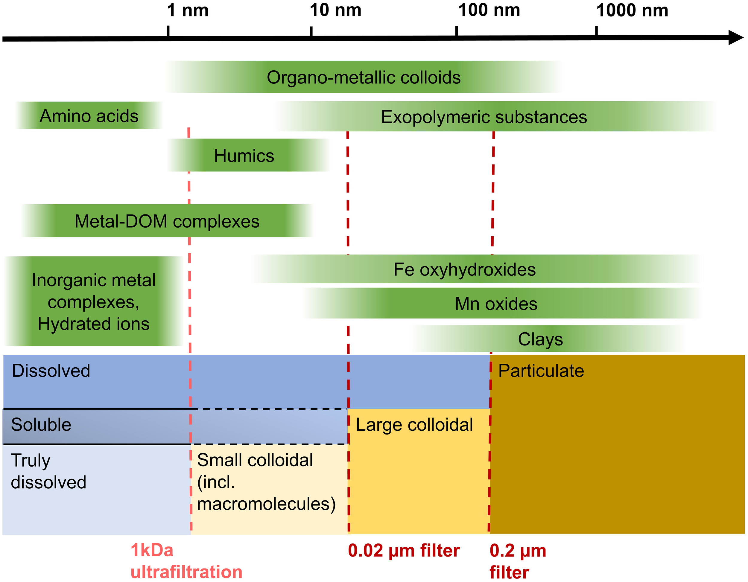
Overview of filtration steps, size classes as defined in this study, and examples of organic and inorganic compounds within this size schematic. Size information based on (Lead and Wilkinson, 2006). We use the size class “small colloidal” for all colloids and molecules between 1 kDa and 0.02 µm.
The size fractionation serves as a basis to unravel the complexity of the dissolved pool and the differentiation between the physical species is an important prerequisite for diffusion calculations, flux models, understanding and predicting chemical reactivity, and bioavailability assessments. Depending on the physical and chemical speciation, metals behave differently during biogeochemical cycling and speciation can also influence toxicity. While physical speciation does not directly relate to bioavailability, it can serve as an indication which chemical forms are likely present within the physical size pool (Figure 1). Additionally, exposure routes differ for soluble, colloidal, and particulate metals and will affect fauna in different ways (Simpson and Spadaro, 2016; Hauton et al., 2017). It is therefore a useful basis for ecotoxicological studies e.g., in the context of deep-sea mining, to know in which forms the metals are present in the natural system.
A further driver is to understand trace metal diffusion across the sediment-water-interface (SWI) that can impact bottom water trace metal cycling (Huerta-Diaz et al., 2007; Homoky et al., 2011). Depending on their physical and chemical speciation (e.g., free ion, organic complex, colloid), diffusion and reaction properties for metals will differ (Homoky et al., 2016; Baeyens et al., 2018). Diffusion coefficients that have been empirically determined for free ions might not be appropriate for colloidally bound metals and introduce uncertainty to benthic flux calculations (Homoky et al., 2016; Somes et al., 2021). Scally et al., 2006 discovered that the diffusion coefficients in diffusive gradients in thin film decreased as the ligand size increased and that diffusion coefficients for metal-ligand complexes were 20-30% lower than for simple organic ligands such as diglycolic acid or nitrilotriacetic acid. The much greater retardation of metals complexed by e.g., humic and fulvic substances compared to uncomplexed or inorganically complexed metals has been observed (Zhang and Davison, 1999; Scally et al., 2006; Balch and Guéguen, 2015) and diffusion coefficients are only 10-20% of the values of uncomplexed or inorganically complexed metals. Especially in oxic settings, colloidal species of e.g., Mn and Fe as well as associated metals will play an important role as a source of these elements from the pore water to the water column (Homoky et al., 2021) but are often still neglected in model simulations (Somes et al., 2021). Providing data on the fraction of colloids for a range of metals in abyssal, oxic pore waters will contribute significantly to the improvement of our understanding of benthic fluxes in these areas, especially because the abyssal deep ocean represents the largest area of pore water-seawater exchange (Homoky et al., 2016; Homoky et al., 2021).
Physical speciation of many trace metals is related to the redox conditions in the sediments: Mn and Fe can form (oxyhydr)oxide colloids in oxic pore waters, which are in turn sorbents for many other trace metals. Cationic metals such as Co and Ni are predominantly present as free ions or CoCl+/NiCl+ complexes in seawater when they are not organically complexed (Ćosović et al., 1982; Ellwood and Van den Berg, 2001; Koschinsky and Hein, 2003), and are often associated with Mn oxides (negative surface charge) (Shaw et al., 1990; Koschinsky and Halbach, 1995; Paul et al., 2018). Manganese and Fe colloids are not stable under reducing conditions for these elements (Froelich et al., 1979). The oxyanion-forming metals Mo, V, U and the metalloid As are mostly present as negatively charged complexes and stable in their oxidized, soluble forms: Mo6+ (as MoO42-), V5+ (as H2VO4- or HVO42-), U6+ (as UO2(CO3)34-) and As5+ (HAsO42-) (Andreae, 1979; Neff, 2002; Beck et al., 2008). Under reducing conditions, As can be desorbed from Mn and Fe oxides or released due to reduction of these host phases (Telfeyan et al., 2017). Arsenic readily adsorbs to positively charged Fe oxyhydroxides (Koschinsky and Halbach, 1995) when present as oxyanions, while adsorption onto negatively charged Mn oxides has mostly been observed at edge sites of Mn minerals (Schacht and Ginder-Vogel, 2018).
Trace metal size fractionation is increasingly assessed in the oceanic water column (Nishioka et al., 2001; Oldham et al., 2017; Jensen et al., 2020). Less frequently studied are the pore waters, which are traditionally more time-consuming to sample, especially under ultra-clean conditions, and sample volume is limited. The small volumes are a limitation for sequential filtration techniques to assess the different size pools of the dissolved fraction (colloidal, soluble, truly dissolved) because for ultrafiltration (1-10 kDa) usually 100 milliliters to liters are necessary. The typical focus in pore water has been on Fe because there is a large interest in its role as a bio-essential and climate influencing element (Homoky et al., 2011; Homoky et al., 2016; Homoky et al., 2021), but other bio-essential (Mn, Cu, Co, Ni, Cd) or potentially toxic (Cu, Mn, As, Cd) trace metals show a variety of behaviors. In our study, we present a comprehensive overview of the soluble and colloidal distributions of Mn, Co, Ni, Fe, Cu, V, U, Mo, As, and Cd in oxic to suboxic deep-sea pore waters.
2 Methods
2.1 Sampling
Samples were taken during RV SONNE cruise SO268 in the period between February and May 2019 as part of the JPI Oceans MiningImpact project (Haeckel and Linke, 2021). The cruise covered the German and Belgian license areas for manganese nodule prospection in the Clarion Clipperton Zone (CCZ), central equatorial Pacific (Figure 2; Table 1).
Figure 2
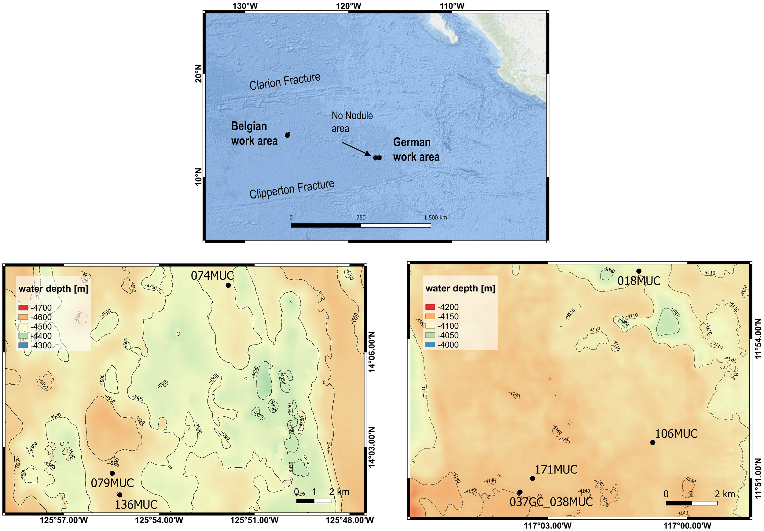
Map of sampling locations in the Belgian (left) and German (right) license areas in the CCZ. The ‘No Nodule’ area is not shown in a close-up map. Sources for ESRI Ocean base map: Esri, GEBCO, NOAA, National Geographic, DeLorme, HERE, Geonames.org, and other contributors. Close-up map data is from the multibeam echosounder EM 122 from RV SONNE (Gazis, 2020a; Gazis, 2020b). Maps were created with QGIS.
Table 1
| Sample ID | Work area | Latitude [N] | Longitude [W] | Water depth [m] |
|---|---|---|---|---|
| SO268 Leg 1 | ||||
| 018MUC | German license area – Trial site | 11° 55.454’ | 117° 01.039’ | 4092 |
| 037GC | German license area – Reference site | 11° 50.708’ | 117° 03.593’ | 4132 |
| 038MUC | German license area – Reference site | 11° 50.686’ | 117° 03.612’ | 4130 |
| 074MUC | Belgian license area – Trial site | 14° 08.105’ | 125° 51.819’ | 4509 |
| 079MUC | Belgian license area – Reference site | 14° 02.187’ | 125° 55.471’ | 4535 |
| SO268 Leg 2 | ||||
| 106MUC | German license area – Dredge site (pre-impact) | 11° 51.773′ | 117° 00.740′ | 4122 |
| 136MUC | Belgian license area – Reference site | 14° 01.505′ | 125° 55.234′ | 4542 |
| 157GC | German license area – No Nodule site | 11° 50.976′ | 117° 22.956′ | 4275 |
| 158ROV-PUC 8 | German license area – No Nodule site | 11° 50.971′ | 117° 22.930′ | 4278 |
| 171MUC | German license area – Reference site | 11° 51.003′ | 117° 03.323′ | 4122 |
Overview of cores sampled for trace metal analyses and MiningImpact project related work areas.
Surface sediments (ca. 20-30 cm) were collected with a multicorer (MUC) or ROV push core (ROV-PUC) and sediments down to ca. 5 m depth with a gravity corer (GC). Surface sediments up to ca. 75 cm were lost at the top of the GCs. The loss was variable among cores and could not be reconstructed. Therefore, all data shown here for the GCs are sampling depth within the core. Sediment cores were immediately transferred into the cold room of RV SONNE (4-7°C). The MUC bottom waters overlying the collected sediments in the liners were sampled with 0.1 M suprapure HCl and deionized water (DI; 18.2 MΩ•cm) pre-cleaned syringes and directly filtered through 0.2 µm polyethersulfone (PES; Chromafil, Macherey-Nagel) syringe filters that were pre-cleaned with DI during SO268 Leg 1 and with 0.1 M suprapure HCl and DI during SO268 Leg 2 (Table 1). Syringes were rinsed with samples first and the first drops of sample going through the filter were discarded. To sample the pore water, sediment was transferred into acid (technical grade 2% HNO3 and 0.2% HF) and DI cleaned 50 mL centrifuge tubes with acid (10% HNO3) and DI cleaned plastic spatulas. MUCs and the ROV PUC were sampled in 2 – 4 cm layers. For higher resolution dissolved and soluble pool comparisons, such as 136MUC and 171MUC, samples from the same depth intervals of two MUC liners were pooled to acquire sufficient pore fluids. Similarly looking cores were chosen. GCs were sampled upon eye inspection in different layers, approx. 3 samples per 1 m core section. All samples were centrifuged at 4°C, 2465 x g (3500 rpm), for 40 minutes to separate the pore water from the solid phase. The supernatant pore water was subsequently filtered through 0.2 µm PES syringe filters that were pre-cleaned with DI during SO268 Leg 1 and with 0.1 M suprapure HCl and DI during SO268 Leg 2 (Table 1). The syringes were always pre-cleaned with 0.1 M suprapure HCl and DI. Syringes were rinsed with sample first, which was discarded, and the first drops of sample filtered through the syringe filter were also discarded. For 0.02 µm filtration, sample was taken from the 0.2 µm filtrate with a clean syringe after pre-rinsing with 0.2 µm sample, and filtered through Anotop syringe filters (alumina based Anopore membrane; Whatman) directly after the 0.2 µm filtration was completed. This is well within the 24 h time range recommended by Jensen et al. (2020) to get reliable soluble and dissolved metal concentrations. Anotop filters were cleaned with DI during SO268 Leg 1 and 0.015 M suprapure HCl and DI during SO268 Leg 2. Filtration of oxic samples was performed in a clean bench. Based on the data of onboard ex-situ oxygen measurements (Haeckel and Linke, 2021), samples from suboxic GC sediments were filtered in a glove tent filled with nitrogen. Sediment subsampling of the 1 m GC liner sections was performed in ambient air as is standard procedure for GCs and has been successfully carried out in previous studies (Volz et al., 2018; Paul et al., 2019). Diffusion of oxygen is only a few mm in the 2-3 hours of sampling (Paul et al., 2019) and the few mm of air-exposed surface sediment were removed prior to sampling the sediment into the centrifuge tubes.
Trace metal samples were acidified with 1.5 µL ultrapure HCl per 1 mL sample to ~pH 1.8. Trace metal samples were stored in LDPE bottles or 5 mL PP vials cleaned with detergent, technical grade 2% HNO3 and 0.2% HF, and 1 M suprapure HCl and DI, at ca. 4-9°C until analysis.
2.2 Analytical
2.2.1 Direct ICP-MS analysis
Cadmium, U, V, Cu, As, and Mo, as well as Mn and Co in pore waters from the GCs, were determined at Jacobs University Bremen (JUB, Germany, now Constructor University) by single quadrupole Inductively-Coupled Plasma - Mass Spectrometry (ICP-MS, Perkin Elmer NexION 350X) coupled to an apex Q desolvating nebulizer (Elemental Scientific, ESI) for increased sensitivity and decreased background. Concentrations of these elements are sufficiently high (in comparison to blanks and the sensitivity of the ICP-MS) to be analyzed directly. Additionally, V, Mn, Co, Cu, As, and Mo were measured in the kinetic energy discrimination (KED) mode using He gas for the minimization of polyatomic interferences. Pore-water and bottom water samples were diluted 80-100 times and Ru was used as internal standard to correct for machine drift. Calibration standards and instrument blanks were matrix matched to the diluted pore-water samples with NaCl (Merck, suprapure). For quality control, certified reference materials (CRMs) for seawater NASS-7 and estuarine water SLEW-3 (both National Research Council of Canada; www.nrc-cnrc.gc.ca) were measured with the samples at the same dilution as the samples. As no pore-water CRM exists, an in-house pore water mix from the Peru Basin with realistic element concentrations for pore water was measured in every run. Accuracy for NASS-7 and/or SLEW-3 was within 5% for U, V, As, Mo, and Mn, 10% for Cu, 17% for Co and 30% for Cd. Precision was largely within 2-10% for all elements depending slightly on the CRM used, except for Co, Cu and As, which were for some CRMs 12-25%. For details on the detection limit (LOD) and CRM measurements see Table 2. Replicate analyses of 12 samples on different days showed a general agreement within ca. 8%, except for Cu and As (ca. 15%).
Table 2
| LOD [µg/kg] | LOD [nmol/kg] | NASS-7 [µg/kg] | SLEW-3 [µg/kg] | In-house [µg/kg] | ||||||
|---|---|---|---|---|---|---|---|---|---|---|
| 1certified 2reference | average measured | n | 1certified 2information | average measured | n | average measured | n | |||
| 0.002-0.03 | 0.018-0.27 | Cd | 0.0157 ± 0.00161 | 0.025 ± 0.007 | 5 | 0.047 ± 0.0041 | 0.061 ± 0.014 | 9 | 0.190 ± 0.004 | 9 |
| 0.001-0.04 | 0.004-0.02 | U | 2.81 ± 0.161 | 2.90 ± 0.22 | 9 | 1.82 | 1.75 ± 0.30 | 9 | 2.93 ± 0.08 | 9 |
| 0.007-0.31 | 0.14-6.09 | V | 1.27 ± 0.082 | 1.30 ± 0.09 | 9 | 2.54 ± 0.311 | 2.63 ± 0.12 | 9 | 7.52 ± 0.31 | 9 |
| 0.10-1.14 | 1.82-20.8 | Mn | 0.74 ± 0.061 | <LOD | 1.59 ± 0.221 | 1.58 ± 0.02 | 2 | 2.79 ± 0.17 | 2 | |
| 0.003-0.017 | 0.051-0.29 | Co | 0.0143 ± 0.00141 | <LOD | 0.040 ± 0.0101 | 0.033 ± 0.003 | 2 | 0.043 ± 0.011 | 2 | |
| 0.03-0.3 | 0.47-4.72 | Cu | 0.195 ± 0.0141 | <LOD | 1.53 ± 0.121 | 1.68 ± 0.39 | 12 | 4.10 ± 0.35 | 12 | |
| 0.01-1.7 | 0.13-22.7 | As | 1.23 ± 0.062 | 1.20 ± 0.16 | 9 | 1.34 ± 0.091 | 1.38 ± 0.16 | 8 | 1.97 ± 0.50 | 9 |
| 0.08-0.32 | 0.83-3.34 | Mo | 9.10 ± 0.401 | 9.53 ± 0.31 | 9 | 5.12 | 4.90 ± 0.33 | 9 | 14.1 ± 0.53 | 9 |
Overview of LOD and CRM measurements at Jacobs University Bremen.
Each CRM was measured several times per run and averages from each run were used to calculate the CRM average shown in the table. The in-house standard was measured once per run. n= number of ICP-MS runs.
2.2.2 SeaFAST offline preconcentration
Selected cores from Leg 2 (Table 1) which were sequentially filtered throughout the core (106MUC, 136MUC, 158ROV PUC8, and 171MUC) were additionally analyzed for Mn, Fe, Co, and Ni using the much more time intensive and costly seaFAST preconcentration. The samples were measured at GEOMAR (Kiel, Germany) with a high-resolution sector field ICP-MS (ElementXR, Thermo Scientific) after offline preconcentration using a SeaFAST (Elemental Scientific, ESI). The method was based on Rapp et al., 2017). In brief, samples were diluted with subboiling HNO3-DI of pH ~1.6 and loaded onto a chelating resin column (Nobias, ESI CF-N-0200 SeaFAST 200 µL) after buffering to pH 8.5 with acetic acid (HAc, ROMIL UpA) and ammonia (NH3, ROMIL UpA, 3 M) in the SeaFAST. Samples were subsequently eluted with 1 M HNO3. Prior to column loading, samples were UV digested for 4 h to destroy organic ligands that may prevent especially Co from quantitative loading onto the chelating resin. All elements were quantified by external calibration. Calibration standards were prepared in seawater from SO268 and preconcentrated with the SeaFAST prior to ICP-MS measurement. For quality control, CRMs for seawater CASS-6 and estuarine water SLEW-3 (both National Research Council of Canada; www.nrc-cnrc.gc.ca) were measured with the samples (Table 3). Accuracy was within 3-6% for Mn, Fe, Co, and Ni for CASS-6 and between 3-13% for SLEW-3. Precision was 3-7% for all elements.
Table 3
| LOD [nmol/L] | LOD [µg/L] | CASS-6 [µg/L] | SLEW-3 [µg/L] | |||||
|---|---|---|---|---|---|---|---|---|
| certified | average measured | n | certified | average measured | n | |||
| 0.013-0.198 | 0.0007-0.0109 | Mn | 2.22 ± 0.12 | 2.10 ± 0.47 | 2 | 1.61 ± 0.22 | 1.66 | 1 |
| 0.082-1.28 | 0.0046-0.072 | Fe | 1.56 ± 0.12 | 1.48 ± 0.07 | 3 | 0.568 ± 0.059 | 0.626 | 1 |
| 0.002-0.009 | 0.0001-0.0005 | Co | 0.0672 ± 0.0052 | 0.0653 ± 0.0019 | 3 | 0.042 ± 0.010 | 0.0474 | 1 |
| 0.081-0.494 | 0.0048-0.029 | Ni | 0.418 ± 0.04 | 0.394 ± 0.03 | 3 | 1.23 ± 0.07 | 1.32 | 1 |
Overview of LOD and CRM measurements at GEOMAR.
Each CRM was measured three times at the beginning of a sequence. The average per sequence was used for the overall calculation shown here. n=number of sequences.
2.2.3 Blanks and reporting
Field blanks (ship DI filtered the same way as the samples) were all considerably below the LOD for all elements except Mn, Fe, and Co and for the Anotop filters for Ni. Blanks were not subtracted from the samples because they were very variable. Anotop 0.02 µm blanks were generally 10-20 times higher than 0.2 µm PES blanks. No substantial difference for the filter blanks was noticed for the elements presented here for both cruise legs (acid vs. only DI cleaning), except for Co, for which the blanks of acid cleaned PES syringe filters were about 10 times lower.
The results for 0.02 µm filtration samples that were considerably higher than for 0.2 µm filtrations were excluded because the most likely explanation for this was contamination during the sequential filtration. This was mostly the case for Mn and Fe data: Of a total of 23 0.02 µm filtered samples analyzed for Mn, Fe, Co, and Ni at GEOMAR, 3 samples Mn and 1 sample Fe, Co, and Ni from 106MUC, 5 samples Fe, 4 samples Mn, and 3 samples Co and Ni from 136MUC, and 1 sample Mn and Fe from 171MUC were affected. The remaining 15 Mn, 17 Fe, and 19 Co and Ni samples were determined to be reliable because of the consistency of the data within cores, between cores, and in comparison to the 0.2 µm filtrates. The 51 0.02 µm samples analyzed at JUB for Cd, Cu, V, As, U, and Mo in the MUCs and the 8 samples analyzed for Mn, Co, and Cu in the GCs did not show any contamination issues. Solely two of these samples had calibration or interference problems for Mo, Cd, and U and were therefore ignored. Additionally, data for samples that could not be reproduced within the same institute and were extraordinarily high during the second measurement were also discarded due to possible contamination during sample handling (n=2).
Colloidal concentrations ([cMetal]) were calculated from the concentration difference [dMetal]-[sMetal], with [dMetal] being the dissolved metal concentration and [sMetal] being the soluble metal concentration.
3 Results
Dissolved Mn, dCo, dNi, dCu, and dV displayed a peak in the upper 6 cm, with highest concentrations usually at 2 cm depth, just below the SWI (Figures 3–5).
Figure 3
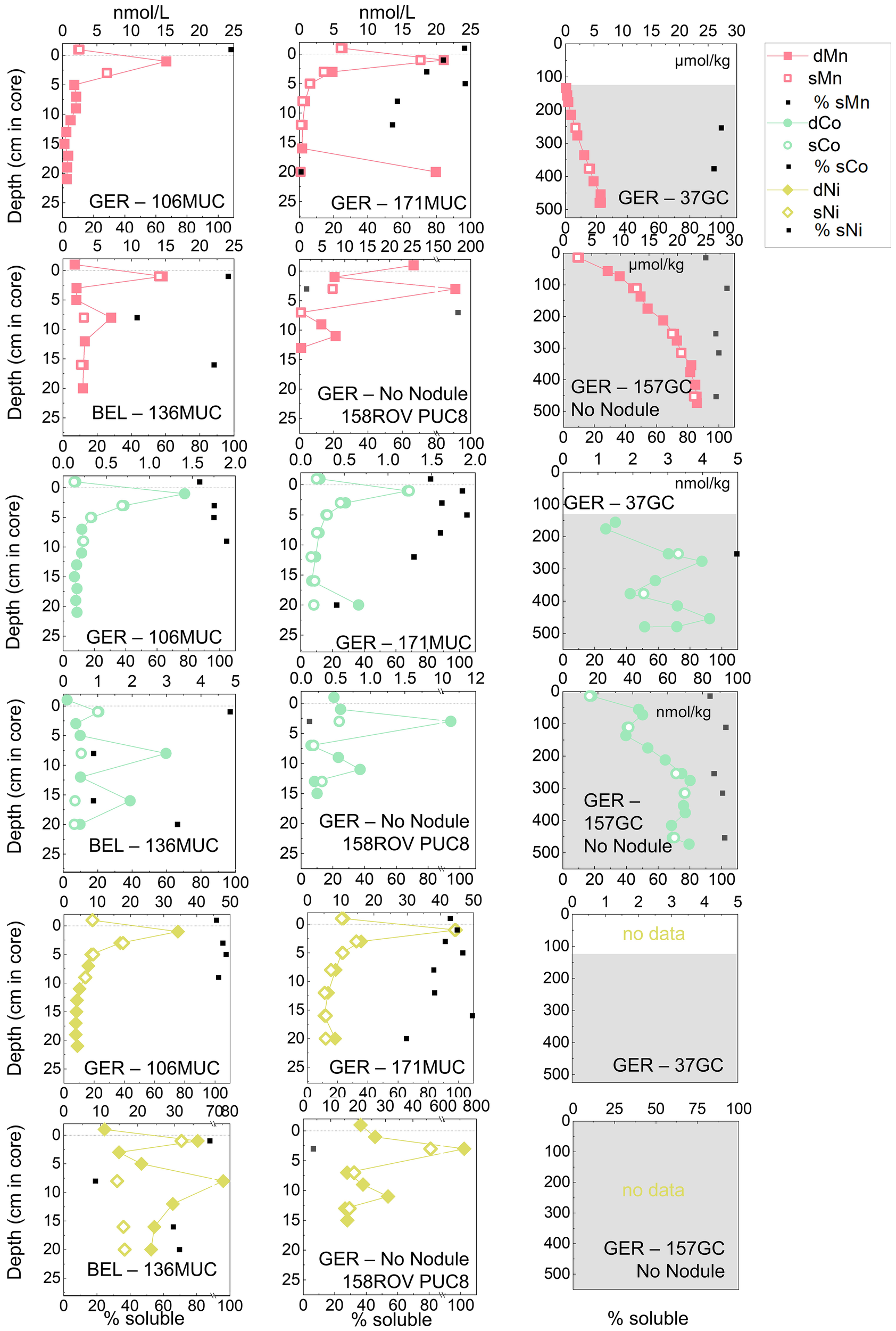
Dissolved (< 0.2 µm) and soluble (< 0.02 µm) Mn, Co, and Ni concentrations in pore waters of the German (GER) and Belgian (BEL) license areas. The difference between dissolved (< 0.2 μm) and soluble (< 0.02 μm) is shown as the percentage of sMetal of dMetal. The uppermost value of the MUC/PUC is the bottom water. The dotted line indicates the SWI. Note different y-axis for GCs and MUCs/PUC. The grey areas in the GC plots indicate suboxic conditions, correlating with the increase of dMn concentrations. For 37GC, Mn and Co in the oxic pore water were below the detection limit 20.8 and 0.29 nmol/kg, respectively.
Figure 4
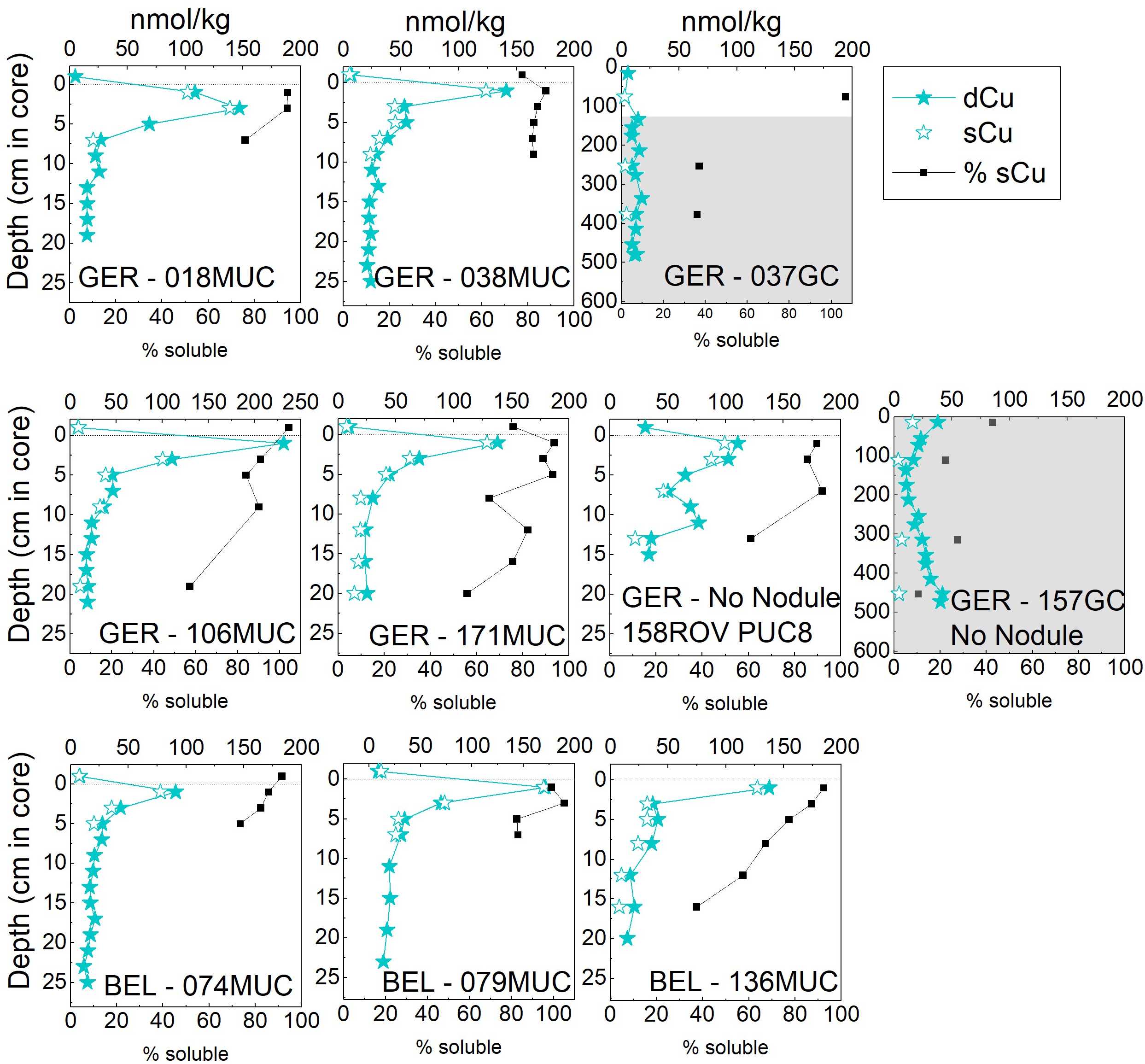
Dissolved (< 0.2 µm) and soluble (< 0.02 µm) Cu concentrations in pore waters of the German and Belgian license areas. The difference between dissolved (< 0.2 µm) and soluble (< 0.02 µm) is shown as the percentage of sCu of dCu. The uppermost value of the MUC/PUC is the bottom water. The dotted line indicates the SWI. Note different y-axis for GCs and MUCs/PUC. The grey areas in the GC plots indicate suboxic conditions. dCu data for 074MUC and 079MUC from (Paul and Koschinsky, 2021a; Paul and Koschinsky, 2021b).
Figure 5
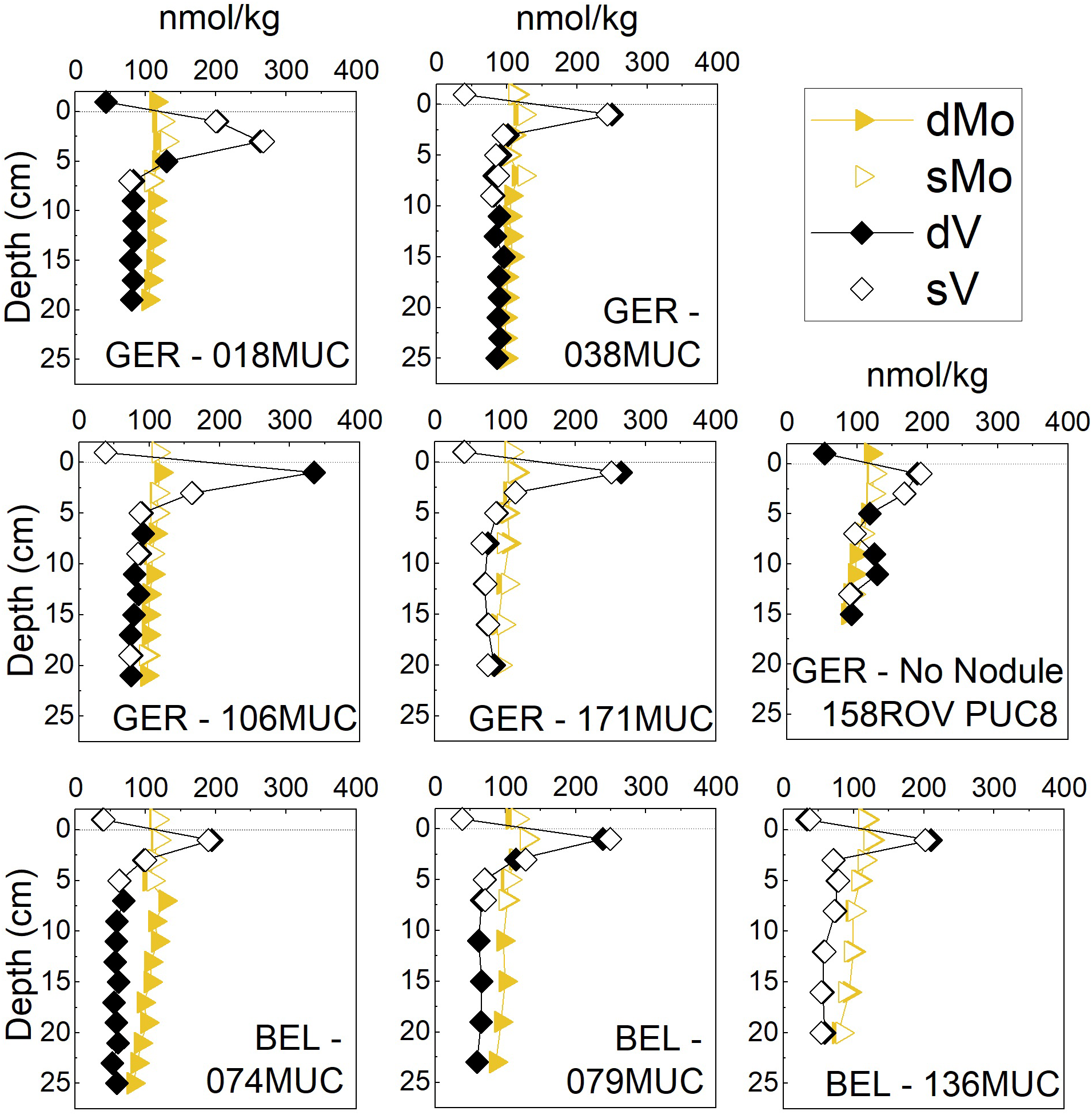
Dissolved (<0.2µm) and soluble (<0.02µm) concentrations of oxyanion forming metals V and Mo in the German (GER) and Belgian (BEL) license areas surface pore waters (ca. 25 cm). The uppermost value of the MUC/PUC is the bottom water. The dotted line indicates the SWI.
MUC bottom water dMn was 1.7 nmol/kg in the Belgian area and variable within the German area between 2-6 nmol/L and up to 25 nmol/L at the “No Nodule” site (Figure 3). In comparison, pore waters were enriched with 15-21 nmol/L in the Belgian and German areas and up to 177 nmol/L at 2-4 cm depths at the “No Nodule” site. With depth, dMn decreased to ca. 2-3 nmol/L in the Belgian area and to < 1 nmol/L in the German area, but remained highly variable at the “No Nodule” site (Figure 3). Dissolved Co and Ni showed similar trends, with bottom water dCo of 0.11-0.22 nmol/L and dNi of 9-11 nmol/L at the Belgian and German areas, except for higher concentrations at the “No Nodule” site with 0.48 nmol/L dCo and 21 nmol/L dNi. Pore-water concentrations were elevated up to 1.4 nmol/L dCo and 45 nmol/L dNi, with exceptionally high concentrations of 10.5 nmol/L dCo and 726 nmol/L dNi at 2-4 cm depth at the “No Nodule” site. Down to ca. 20 cm depth, concentrations of dCo and dNi remained higher in the Belgian area (~ 0.5 nmol/L dCo, 20-30 nmol/L dNi) compared to the German area (~ 0.1-0.2 nmol/L dCo, 4-10 nmol/L dNi), except for the “No Nodule” site (Figure 3). In the suboxic zone down to 5 m depths, Mn and Co concentrations increased substantially, Mn to the µmol/kg range and Co to up to 73 nmol/kg (Figure 3). Concentrations in the suboxic zone are considerably higher at the “No Nodule” site (157GC) compared to the other core from the German area (37GC). The “No Nodule” site therefore clearly deviates from the general trends in the German and Belgian work areas.
Manganese, Co, and Ni were predominantly present in the soluble phase (< 0.02 µm) in the bottom water (sMn 96-108%, sCo 82-87%, sNi 94-101%) and upper 10 cm of the oxic pore waters (sCo 88-105%, sNi 84-107%), with Mn showing the largest variability in the pore waters (sMn 57-97%, 158ROV PUC8 2-4 cm as an outlier with only 4% sMn) (Figure 3). Below 10-15 cm, the concentrations of sMn decreased to 54%, sCo and sNi to ca. 70%. The large peaks below 5 cm were largely colloidal while the soluble profiles were smooth (e.g., 136MUC at 8 cm, Figure 3). In the suboxic zone, however, dissolved and soluble concentrations of Mn and Co were indistinguishable (GCs Figure 3). Nickel was not determined for the GCs.
Bottom water dCu concentrations were on average 12.3 ± 9.3 nmol/kg and 8.5 ± 0.3 nmol/kg in the German and Belgian area, respectively (Figure 4). Concentrations for dCu maxima in the subsurface pore water were between 103 and 232 nmol/kg at the German area and slightly lower between 91 and 172 nmol/kg at the Belgian area. Copper concentrations decreased with depth and dCu was generally below the detection limit (ca. 3 nmol/kg) for the GCs in the Belgian area and below 20-50 nmol/kg in the German area GCs. While ca. 80-100% of dCu was sCu in the top 5-10 cm at all sites, at around 10 cm depth sCu made up only ca. 60% of the dCu pool. The colloidal pool between 0.02 and 0.2 µm gained importance and was the dominant dCu pool with over 50% cCu below ca. 15 cm in the Belgian area and ca. 1 m in the German area (Figure 4). The bottom water cCu pool was in the same range as the cCu pool in the upper ca. 10 cm with sCu 76-104% of dCu except for one outlier of 131% for 79MUC, which needs to be treated with caution and was therefore also not shown in the % soluble plot in Figure 4.
Vanadium concentrations in the bottom water were 43.1 ± 5.6 nmol/kg in the German area and 38.7 ± 0.7 nmol/kg in the Belgian area. Subsurface maxima of dV in the upper 2 cm were considerably enriched with 185-334 nmol/kg and 195-239 nmol/kg in the German and Belgian areas, respectively. Dissolved V concentrations then decreased to 70-90 nmol/kg with depth in the German area and to 55-75 nmol/kg in the Belgian area (Figure 5).
The subsurface peak was less clearly visible for dFe, but all cores showed a peak in the upper 2-4 cm (Figure 6). Dissolved Fe concentrations generally varied between 4-40 nmol/L. The two maxima of ca. 350 nmol/L (171MUC) and 3.5 µmol/L (158ROV PUC8) were only present in the dissolved fraction but not in the soluble fraction, therefore they must be due to Fe colloids present at specific layers (Figure 6).
Figure 6
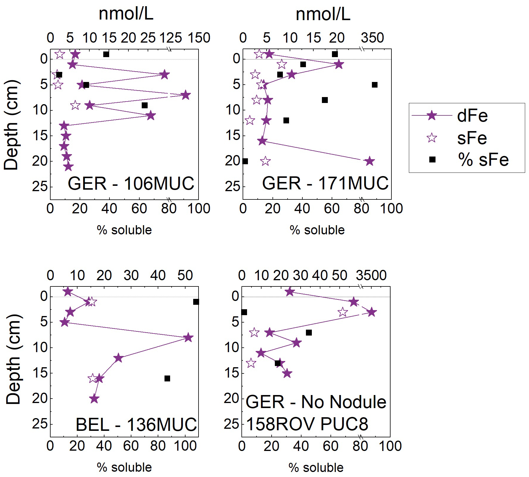
Dissolved (< 0.2 µm) and soluble (< 0.02 µm) Fe concentrations in pore waters of the German (GER) and Belgian (BEL) license areas. The difference between dissolved (< 0.2 μm) and soluble (< 0.02 μm) is shown as the percentage of sFe of dFe. The uppermost value of the MUC/PUC is the bottom water. The dotted line indicates the SWI. Iron was not determined for the GCs.
The subsurface peak was less pronounced for As, but all cores except the one from the ‘No Nodule’ site also show a peak-trend in the upper 2-4 cm (Figure 7). Dissolved and soluble Cd pore-water concentrations were considerably enriched (ca. 1.3-2 nmol/kg) throughout the upper ca. 25 cm compared to bottom seawater [average 1.01 ± 0.04 nmol/kg and 0.88 ± 0.04 nmol/kg in the German and Belgian areas, respectively (Figure 8)]. The pore-water Cd concentrations in the German area were on average higher (1.66 ± 0.17 nmol/kg) compared to the Belgian area (1.33 ± 0.12 nmol/kg).
Figure 7
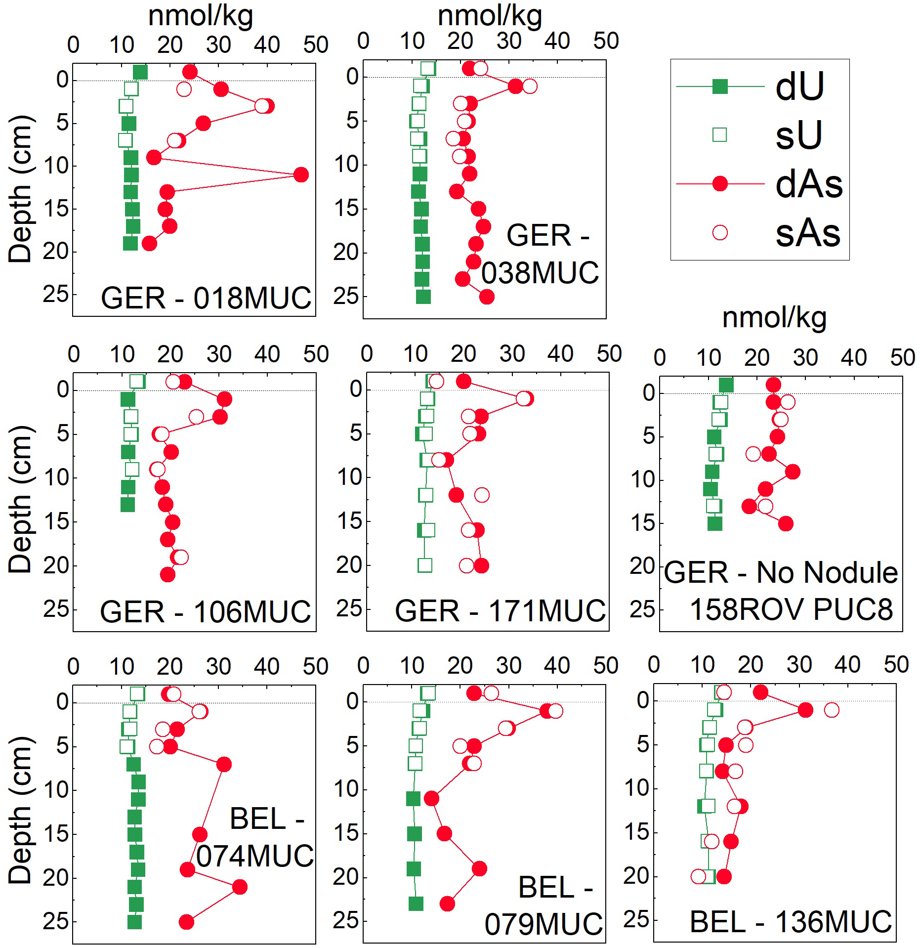
Dissolved (<0.2µm) and soluble (<0.02µm) concentrations of oxyanion forming metal(loid)s U and As in the German (GER) and Belgian (BEL) license areas surface pore waters (ca. 25 cm). The uppermost value of the MUC/PUC is the bottom water. The dotted line indicates the SWI.
Figure 8
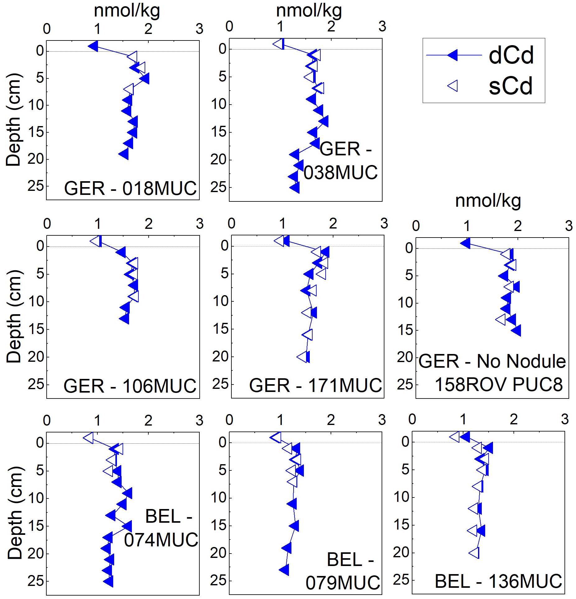
Dissolved (<0.2µm) and soluble (<0.02µm) concentrations of Cd in the German (GER) and Belgian (BEL) license areas surface pore waters (ca. 25 cm). The uppermost value of the MUC/PUC is the bottom water. The dotted line indicates the SWI.
At all sites, Mo and U displayed straight pore-water profiles in the surface pore waters (upper ca. 25 cm) (Figures 5 and 7); Mo in the same concentration range (ca. 90-120 nmol/kg) as MUC bottom water (ca. 112-114 nmol/kg) in both work areas and U at slightly lower concentrations (ca. 12 nmol/kg) compared to seawater (ca. 13 nmol/kg). However, Mo concentrations decreased steadily with depth by 13-35%, most strongly at the ‘No Nodule’ site and the Belgian area.
The dissolved and soluble concentrations for V, As, Cd, Mo, and U were the same and within analytical precision and no major differences in concentration and profile pattern could be discerned in the oxic surface pore waters (Figures 5, 7, 8).
Overall, most metals presented here (Mn, Co, Ni, Fe, Cu, V, Cd) were enriched in oxic pore waters compared to bottom seawater. The enrichment was slightly more variable in the German area but the upper 2 cm peak concentrations were also usually higher in the German compared to the Belgian area. The “No Nodule” site in the German area displayed most variable concentrations for Mn, Co, Ni, and Cu. The colloidal pool (0.02-0.2 µm) increased with depth for Mn, Co, Ni, and Cu.
4 Discussion
4.1 Subsurface Mn, Co, and Ni peaks
The pore waters in surface sediments (< 25 cm) were oxic and aerobic respiration largely controlled organic matter degradation in the sediments shallower than 1 m (Volz et al., 2018). Suboxic conditions (absence of oxygen, co-occurrence of nitrate and elevated (µM range) pore-water Mn, absence of sulfide) occurred at depths > 1 m and were variable between the study sites (Volz et al., 2018). The area was characterized by low but variable inputs of organic matter and the total organic carbon (TOC) content in surface sediments was 0.2-0.6 wt.% (Volz et al., 2018). Reductive dissolution of Mn oxides only occurred at depths of ca. 1 to 10 m (Volz et al., 2018) which is also indicated by increasing Mn concentrations to the µmol/kg range for two examples from the German area (GCs Figure 3). Manganese and Fe (oxyhydr)oxide colloids must therefore be stable in the oxic CCZ surface pore waters.
Manganese, Co, and Ni showed similar depth profiles (Figure 3) because Co and Ni are often adsorbed or incorporated onto or into Mn oxide minerals and then these elements are cycled together between the solid and dissolved as well as between the colloidal and soluble phase (Klinkhammer, 1980; Sawlan and Murray, 1983; Shaw et al., 1990; Koschinsky and Halbach, 1995). All three elements displayed a peak in the upper 6 cm in the dissolved and soluble fractions, with highest concentrations at ca. 2 cm, just below the SWI (Figure 3). This is due to the release of these metals during organic matter degradation, which has been shown for Cu and V in oxic pore waters (Klinkhammer, 1980; Heggie et al., 1986; Shaw et al., 1990; Paul et al., 2018), but rarely for Mn, Co, and Ni, and the exact mechanisms were not discussed in these previous publications. In the case of Mn, Co, and Ni, this peak was often not discoverable, potentially due to a lack of analytical sensitivity or because studies were mostly conducted in areas with a more condensed redox zonation (e.g., shelves) where the Mn, Co, and Ni peaks at the oxic-suboxic boundary dominated the profiles (Klinkhammer, 1980; Sawlan and Murray, 1983; Shaw et al., 1990). Heggie et al. (1986) observed Mn and Ni peaks in oxic pore waters at the SWI. They attributed the Mn peak to the reduction of solid-phase Mn oxides through dissolved organic matter (Heggie et al., 1986). In the solid phase of the cores presented in this study, Mn was also enriched in the upper ca. 5 cm (Supplementary Figure S1), sometimes considerably in the upper ca. 3 cm, suggesting the presence of Mn micronodules. The solid-phase Mn oxide enrichment can therefore be a source for the reductive Mn (and associated metal) release to the pore waters. Alternatively, in anoxic microenvironments, different forms of Mn oxides that are more easily reduced, or different types of organic matter have been suggested as possible reasons for the metal release at the SWI (Kalhorn and Emerson, 1984; Burdige, 1993). For some organic matter break-down processes, MnO2 might be the preferred electron acceptor even though O2 is present (Kalhorn and Emerson, 1984). Additionally, nitrite maxima of up to 0.6 µM in the uppermost cm were observed at the same sites (Volz et al., in prep; Haeckel and Linke, 2021), suggesting that nitrification or denitrification are occurring, releasing nitrite into the pore water at the same depth as the metals are released. The co-occurrence of nitrite and dMn peaks have previously been reported for the oxygen minimum zones of the Pacific and Arabian Sea, linking denitrification and Mn reduction based on the same noticeable profiles we observed in the CCZ pore waters (Klinkhammer and Bender, 1980; Saager et al., 1989). In the pore waters, nitrite is, however, usually produced by oxidation of ammonia and not by denitrification (Volz et al., 2018). The coinciding nitrite and Mn peaks could therefore also suggest that Mn oxides are utilized for ammonia oxidation (“Mn-anammox”) in these Mn oxide-rich sediments (Mogollón et al., 2016) (Supplementary Figure S1), subsequently releasing nitrite and sMn into the pore waters. The oxidation of ammonia by Mn oxides in the presence of oxygen has been previously described for surface sediments at the Nova Scotia margin (Luther et al., 1997).
Manganese mobilization has also been observed as reprecipitation of Mn oxide on burrow walls from mobilization of oxygen-depleted microenvironments rich in organic matter (Jung and Lee, 1999) and the enrichment of Mn in the shallow subsurface proves this (recent) Mn mobilization, likely in local microenvironments.
In summary, the release of predominantly soluble Mn, Co, and Ni just below the SWI is related to specific conditions and types of Mn oxides or organic matter that allow for reductive dissolution of Mn oxides in this shallow layer of high reactivity.
Once the labile organic matter has been consumed or Mn oxides are not the preferred electron acceptor anymore, the “usual” electron acceptor sequence consisting of O2, NO3-, and MnO2 continues downcore (Froelich et al., 1979). The data from Heggie et al. (1986), redrawn in Burdige (1993) at a higher resolution, clearly show the difference between Mn reduction at the SWI in the oxic sediments and in the “main” Mn reduction zone. As the “normal” Mn reduction zone is reached below 30 cm or at several m in the CCZ (Volz et al., 2018), the small Mn reduction zone at the SWI may play an especially important role in trace metal cycling between the pore water and water column, as diffusion from high concentration suboxic pore waters is not occurring – in contrast to sediments underlying more productive surface waters with a narrow redox zonation. However, the peak at 2 cm suggests a benthic flux to the overlying bottom water, likely fueling polymetallic nodule formation as the oxic diagenetic flux. This flux and its contribution to polymetallic nodule formation has been previously suggested for Mn (Kalhorn and Emerson, 1984; Heggie et al., 1986) but we could here also show it for Co and Ni, two of the major metals of interest in polymetallic nodules (Hein et al., 2013) – to our knowledge for the first time.
4.2 Downcore increase of the colloidal fractions of Mn, Co, and Ni in oxic pore waters
Manganese, Co, and Ni were predominantly present in the soluble phase (sMn 57-97%, sCo 88-105%, sNi 84-107%) in the upper 10 cm of the oxic pore waters (Figure 3). Soluble Mn, Co, and Ni can either be present as the free ions or bound in the small colloidal fraction < 0.02 µm e.g., to organic ligands. The formation of e.g., Mn(III)-ligands which have been previously found in the < 0.02 µm fraction could result from the interaction of Mn with organic matter (Oldham et al., 2017). These Mn(III)-ligands can be produced during ligand-promoted reductive dissolution of Mn oxides (Oldham et al., 2015; Oldham et al., 2020), potentially another pathway for Mn oxide dissolution at the SWI.
Below 10-15 cm, the concentrations of sMn decreased to 54%, sCo and sNi to ca. 70%, indicating that with increasing depth, colloids are becoming more important. Moreover, there were single layers (e.g., 171MUC 20 cm, 136MUC 8 cm) with up to 99% colloidal fraction, which were special microenvironments, potentially in the form of Mn oxides or adsorbed to Fe nanoparticles (also see Figure 6) originating from buried polymetallic nodules in the surrounding sediment. Overall, the dissolved concentrations of all three metals were, however, decreasing with depth. The smallest decrease was visible for sNi and dNi concentrations were higher than dMn and dCo concentrations, indicating that dNi cannot only be controlled by Mn (oxides). A large fraction of dNi is likely controlled by organic ligands, which can be up to 50% in seawater of the tropical South East Pacific Ocean (Boiteau et al., 2016) and might also be important in controlling pore-water Ni. Besides from Mn oxides, Ni is also released during organic matter degradation and silica dissolution at the sediment water interface (Heggie et al., 1986), which would explain the higher concentrations here.
Our results for the colloidal pool in the top 10 cm corroborate findings from a study of contaminated beach sands in which ca. 80-85% Mn and ca. 70% of Co were soluble (Huerta-Diaz et al., 2007) but it needs to be recognized that the setting was considerably different. The dominance of the soluble pool in the top 10 cm also reflects observations for seawater in which only ca. 4% of Mn is in the colloidal phase (1 kDa-0.2 µm) (Wells et al., 2000), in line with our bottom water results (sMn 96-108%). Our results for colloidal Mn at depths > 10 cm were in line with results from Homoky et al. (2011) who found on average 61% of Mn in the colloidal phase in oxic deep-water sediments around the Crozet Islands (Indian Ocean sector of the Southern Ocean). The occurrence and extent of colloidal Mn is therefore likely related to the prevalent lithology. The increase of the colloidal fraction with depth might be related to a decrease of organic ligand concentrations that can bind Mn, Co, and Ni and the substitution by larger inorganic colloids or for Ni also a shift from low to high molecular weight (HMW) organic ligands. Additionally, as suggested above, there might be a thin layer of Mn oxide reduction at the SWI, where the Mn oxide colloids are not thermodynamically stable, but below this ca. 2-6 cm layer, Mn oxide colloids are more stable again. In deeper suboxic pore waters, Mn oxide colloids are not stable (sMn=dMn and sCo=dCo; Figure 3 GCs) due to reductive dissolution of MnO2, as has also been shown e.g., in Homoky et al. (2011).
The suboxic Mn and Co concentrations are especially high at the “No Nodule” site, up to 23 µmol/kg and 73 nmol/kg, respectively. Oxygen penetration is shallowest leading to elevated pore-water Mn (and Co) concentrations below 20 cm (Figure 3). Similar trends have been observed at another “No Nodule” site in the German area (Mewes et al., 2014), highlighting that the geochemistry of the “No Nodule” site is different from the nodule covered areas in the Belgian and German areas. The reasons could, however, not be unraveled yet and there are no clear trends from TOC or sedimentation rate data (Mewes et al., 2014) on what the reasons for the different redox zonation could be.
4.3 Abundant Fe colloids
The dFe profiles (Figure 6) showed some exceptionally high peaks for oxic pore waters (up to 3.5 µmol/L). These maxima were only present in the dissolved fraction but not in the soluble fraction, therefore they must be due to Fe colloids present in specific layers (see 158ROV PUC8 and 171MUC, Figure 6). The sFe profiles were smoother (Figure 6), showing the same subsurface peak as Mn, Co, Ni, Cu, and V. Hence, Fe must also be released during organic matter degradation at the SWI through co-release with other metals or by reductive dissolution of Fe (oxyhydr)oxides in this microenvironment – similar to Mn (section 4.1). Reductive dissolution is likely because sFe was also present but non-reductive dissolution has been suggested to release dFe to oxic pore waters (Homoky et al., 2021). On average, only 40% of dFe was sFe (excluding the peaks where we suspect nanoparticles where the colloidal fraction is even larger), showing that the dominant fraction of dFe in these oxic pore waters was colloidal. This is consistent with findings from Homoky et al. (2021); Homoky et al. (2011), who found a large range of 17-99% of colloidal Fe in oxic pore waters. For the water column, it has been shown that dFe can be mainly colloidally bound, e.g., up to 50% in the North Pacific predominantly below 200 m depth, but this is seasonally and spatially variable throughout the oceans (Nishioka et al., 2001).
Similar to MnO2 colloids, Fe (oxyhydr)oxides and nanoparticles can form and persist in oxic pore waters. In the CCZ sediments investigated here, Fe (oxyhydr)oxides are not even reduced at several meters depth, as only Mn reduction is occurring but not Fe reduction (Heller et al., 2018). Hence, Fe (oxyhydr)oxide colloids can persist even in the suboxic pore waters. In oxic sediments with low organic C supply and a gradually declining O2 gradient [as is the case for the CCZ (Volz et al., 2018)], and therefore slow diagenetic reactions over years/decades/centuries, goethite is the favored Fe (oxyhydr)oxide (Homoky et al., 2011) with higher stability than the less crystalline Fe (oxyhydr)oxide ferrihydrite, which is often assumed to be the dominant Fe (oxyhydr)oxide in marine sediments (Thamdrup, 2000). As this goethite is nanoparticulate with an average size of 5 nm (van der Zee et al., 2003), it is in the colloidal range and can even occur in the operationally defined soluble phase < 20 nm. As colloids tend to aggregate (Honeyman and Santschi, 1988; Jensen et al., 2020), colloidal aggregates exceeding 20 nm, i.e. the 0.02 µm filter pore size, including colloidal goethite, can be found in our 0.02-0.2 µm fraction. In contrast to redox sensitive Fe (oxyhydr)oxides, Fe-bearing clay colloids can exist in suboxic pore waters irrespective of redox conditions. Fe-bearing smectite is a common clay colloid and especially stable in pore waters with high Si (> 500 µM) (Florindo et al., 2003; Homoky et al., 2011). The CCZ pore waters reach concentrations of 400-550 µmol/kg dSi at depth in the GCs from the German area (37GC and 157GC), and around 300-400 µmol/kg in the Belgian area (84GC) (data not shown). These concentrations are sufficiently high to make smectite colloids likely, especially at several meters depth in the GCs. Fe-bearing clay colloids might therefore be important inorganic sorbents for other trace metals once organic ligands are less abundant and MnO2 is not stable anymore. Mineralogical data (not shown) for the sediments revealed that smectite was present in the CCZ surface sediments. The persisting Fe colloids can scavenge metals, some of which (e.g., Co) might have been previously adsorbed to MnO2 colloids. These inorganic Fe colloids are also competing with organic ligands, which become less abundant with depth in the pore water (Paul et al., 2021).
Fe-binding organic ligand analyses in seawater detected 99% Fe(III) bound to organic ligands in the dissolved phase at analytical pH 6.9, which could be slightly less at pH 8 because of different behavior of especially inorganic Fe at the slightly lower analytical pH (Gledhill and van den Berg, 1994). Combined approaches using electrochemical analyses and sequential filtrations (0.4 and 0.02 µm) indicated that the organic ligands are found in the soluble and colloidal pools, but that an additional significant amount of inorganic Fe colloids must be present, which could potentially be Fe (oxyhydr)oxides (Cullen et al., 2006; Fitzsimmons et al., 2015). The differentiation between organic and inorganic ligands/sorbents in seawater has not been straight forward (Boye et al., 2010) and the most prominent and likely explanation is therefore that Fe (oxyhydr)oxides in combination with organic matter are the predominant colloid (Raiswell and Canfield, 2012). There is a continuum of organic-inorganic-nanoparticle-colloid formation and how the metals are bound in each step (Aiken et al., 2011). Processes involving organic and inorganic material include sorption of organic material onto inorganic surfaces and heterogenic precipitation of organic-inorganic clusters/nanoparticles/colloids (Aiken et al., 2011). Adsorption of organic matter onto colloids can change their surface charge and alter their reactivity (Tiller and O’Melia, 1993; Aiken et al., 2011). A complex combination of organic-inorganic ligand complexation of Fe in pore waters is likely and a lot of questions remain about the nature of Fe colloids. More research is needed to explain the variability of the Fe colloidal pool which was also visible in our sFe and dFe data (Figure 6).
4.4 Copper complexation by organic ligands and inorganic colloids
Copper was predominantly soluble in the upper 10 cm of the pore waters and predominantly colloidal at greater depths (Figure 4). Huerta-Diaz et al. (2007) found that the subsurface peak of Cu was only present in the small colloidal fraction (3 kDa-0.45 µm) but not in the truly dissolved phase (< 3 kDa). Therefore, Cu released during organic matter degradation at the SWI appears to be stabilized in the small colloidal size fraction, but likely smaller than 0.02 µm as our results here suggest.
Dissolved and soluble Cu concentrations generally showed the same trends in the depth profiles (Figure 4), but the percentage of soluble Cu decreased with increasing depth at all sites. While ca. 80-100% of dCu was sCu in the top 5-10 cm at all sites, around 10 cm the sCu made up only ca. 60% of the dCu pool. With increasing depth, the fraction of colloidal Cu became dominant, which was already at ca. 15 cm depth in the Belgian area and below roughly 1 m in the German area. This was similar to the behavior of Mn, Co, and Ni, but the colloidal fraction was larger at depth for Cu.
In the German area the colloidal Cu fraction increased at depth, in the suboxic zone (GCs), to up to 90% (157GC, Figure 4). In the Belgian area (136MUC), sCu was already considerably decreased to 23% within the MUC in the oxic pore water. Therefore, the change in Cu complexation was likely not related to redox conditions but to a decreasing and more refractory organic matter content with depth. The shift from soluble to the colloidal pool might be due to the lack of low molecular weight (LMW) organic ligands that keep Cu in the soluble pool. As shown in Figure 1, organic ligands are predominantly present in the soluble fraction. In surface seawater, Cu is up to 99% complexed by organic ligands (Coale and Bruland, 1988). Recently, it was also shown that deep-sea surface pore water Cu is predominantly complexed by organic ligands (Paul et al., 2021), which had previously been reported for Chesapeake Bay pore waters (Skrabal et al., 1997). The analysis of the upper 20-30 cm pore waters showed, however, that the ligand excess decreases with depth similar to dCu profiles, with highest concentrations in the upper 10 cm (Paul et al., 2021). While still > 99% Cu was complexed by organic ligands, the overall ligand concentration decreased with depth. Our findings here corroborate that Cu complexation changes and that while organic ligands (small colloidal size fraction) might become less available, larger inorganic colloids or HMW organic ligands gain importance as Cu ligands. The shift from predominantly soluble to colloidal Cu does not correspond to the redox zonation, so that the physical speciation of Cu might not be related to differences in redox zonation, as it is partly the case for Mn and Fe, but to the availability of small organic ligands. In the deeper layers, Cu could be partially adsorbed to Fe colloids, which are ubiquitous as shown above (Figure 6), but dCu concentrations exceed dFe concentrations, requiring another Cu host-phase or HMW ligand.
4.5 Oxyanion forming metal(loid)s (Mo, V, U, As) and Cd
Pore-water concentrations of As and V in surface sediments were elevated by a factor of 1.3 and 6, respectively, in the upper 2 cm compared to bottom seawater. Vanadium is therefore released during organic matter degradation at the SWI, like Mn, Ni, Co, Fe, and Cu. This is in line with results from other studies and which suggested that V is stabilized by organic material in this layer as V4+ (Wehrli and Stumm, 1989; Emerson and Huested, 1991). The reduced V species (often present as VO2+ or VO(OH)+) is more particle reactive and likely to bind to reactive surfaces (Wehrli and Stumm, 1989), wherefore V could also be released from MnO2 during reductive dissolution at the SWI as explained in section 4.1. The same is possible for As, which can be cycled with Mn as well (Telfeyan et al., 2017) and usually shows a small peak in the upper 2-4 cm (Figure 7).
The dissolved and soluble concentrations for Mo, V, U, As, and Cd were indistinguishable (Figures 5, 7, 8). They are predominantly present as negatively charged complexes and stable in their oxidized, soluble form: Mo6+ (as MoO42-), U6+ (as UO2(CO3)34-), V5+ (as H2VO4- or HVO42-), As5+ (Andreae, 1979; Beck et al., 2008), therefore not found in the colloidal fraction. Vanadium could also be present in the reduced form stabilized by dissolved organic complexes, as described above (Wehrli and Stumm, 1989; Emerson and Huested, 1991). The consistent concentration of dV and sV with depth below ca. 4 cm – unlike for Cu, for which the sCu fraction decreases with depth – could, however, suggest inorganic speciation as more likely. Vanadium does not seem to be affected by changes in organic ligand availability. Vanadium was also found to be in the soluble phase by Huerta-Diaz et al. (2007), while Mo, U, and As were not studied there. In contrast to Huerta-Diaz et al. (2007), Cd is fully soluble in the pore waters studied here, while Cd was up to 60% colloidal in pore waters in the literature comparison conducted by the authors.
5 Conclusions
The oxic deep-sea pore-water samples from the German and Belgian license areas for polymetallic nodule mining in the CCZ showed variable size fractionation for trace metals. Colloidal Fe was present in the pore waters at variable concentrations, while V, Mo, U, As, and Cd were found predominantly in the soluble (< 0.02 µm) fraction. Most interestingly, Mn, Co, Ni, and Cu were completely or mainly soluble in ca. the upper 10 cm, while the percentage of the colloidal fraction increased below 10 cm, most strongly for Cu. These metals must therefore experience a change in complexation and we propose that this is due to the decreasing availability of soluble organic ligands with depth (especially for Cu) and an increase of inorganic complexation e.g., with Fe colloids or a shift to HMW organic ligands. The same might explain the similar distribution of Mn, Co, and Ni. Alternatively, Mn oxides might be less stable in the upper 2-6 cm where a Mn oxide reducing microenvironment might persist. Soluble Mn, Co, and Ni are released to the pore water there and are present at elevated concentrations, fueling the benthic flux of these elements and likely contributing to polymetallic nodule formation. Below this surface layer, Mn oxides incorporating Co and partly Ni form and persist. The distribution of metals between the colloidal and soluble or even truly dissolved phase can have impacts on the diffusion behavior and therefore rates across the SWI (Huerta-Diaz et al., 2007) and needs to be taken into account for flux calculations and further studied. Considering the vastness of the abyssal plains and their large areal contribution to the ocean stresses the importance of these findings to take into account various physical and chemical forms of metals when calculating the global budget of element fluxes across the SWI in the future. To achieve this, diffusion coefficients for various inorganic and organic metal complexes must be experimentally determined first. Furthermore, more research is required in analyzing the organic ligands, nanoparticles, and colloids to fully understand their nature and involvement in particle-solution reactions, which was not possible based on the small sample volumes from this study. The different size fractionations of some metals (e.g., Mn, Cu) in seawater and pore water also showed that the behavior from oxic seawater cannot be easily applied to oxic pore waters and that it is therefore important to thoroughly study pore waters. Understanding the composition of the dissolved pore-water pool is also essential for the assessment of anthropogenic activities – such as deep-sea mining and bottom trawling fisheries – and their impacts on the seafloor environment. Speciation of trace metals will have an influence on the uptake pathways, potential bioavailability, and toxicity of these elements released from the surface pore water by the disturbance. Additionally, the removal of surface sediments during deep-sea mining will impact in which form the metals are released to the bottom seawater: in natural conditions, the here studied metals (except Fe) will be predominantly in the soluble fraction when they diffuse from the pore waters, while post-disturbance an increased colloidal fraction will be part of the benthic flux of Mn, Co, Ni, and Cu until a new equilibrium has been reached because of the increase in the percentage of the colloidal fraction downcore.
Statements
Data availability statement
The datasets presented in this study can be found in online repositories. The names of the repository/repositories and accession number(s) can be found below: Pangaea (Paul et al., 2024).
Author contributions
SP: Conceptualization, Data curation, Formal analysis, Investigation, Writing – original draft. KS: Conceptualization, Investigation, Resources, Writing – review & editing. EA: Writing – review & editing. AK: Conceptualization, Funding acquisition, Supervision, Writing – review & editing.
Funding
The author(s) declare financial support was received for the research, authorship, and/or publication of this article. This work was funded by the German Federal Ministry of Education and Research in the framework of the JPI Oceans project MiningImpact2 (grant number 03F0812G).
Acknowledgments
We thank Pedro Martínez Arbizu (DZMB) and his team, Freia Hauquier (Ghent University), Asmus Petersen, Thorsten Schott, Kristin Hamann (GEOMAR) and Jessica Volz (AWI) for help with MUC and GC sampling. We thank the ROV Kiel 6000 team (GEOMAR) for PUC sampling. We are grateful to Annika Moje (JUB) for help with sampling onboard and cruise preparation, as well as Miriam Wulf and Erika Kurahashi for help in the JUB lab. We thank Tim Steffens and Dominik Jasinski who conducted the SeaFAST measurements at GEOMAR. We also thank the chief scientists Matthias Haeckel and Peter Linke as well as captain Lutz Mallon and the crew of RV SONNE for their tireless support during SO268.
Conflict of interest
The authors declare that the research was conducted in the absence of any commercial or financial relationships that could be construed as a potential conflict of interest.
The author(s) declared that they were an editorial board member of Frontiers, at the time of submission. This had no impact on the peer review process and the final decision.
Publisher’s note
All claims expressed in this article are solely those of the authors and do not necessarily represent those of their affiliated organizations, or those of the publisher, the editors and the reviewers. Any product that may be evaluated in this article, or claim that may be made by its manufacturer, is not guaranteed or endorsed by the publisher.
Supplementary material
The Supplementary Material for this article can be found online at: https://www.frontiersin.org/articles/10.3389/fmars.2024.1339772/full#supplementary-material
References
1
Aiken G. R. Hsu-Kim H. Ryan J. N. (2011). Influence of dissolved organic matter on the environmental fate of metals, nanoparticles, and colloids. Environ. Sci. Technol.45, 3196–3201. doi: 10.1021/es103992s
2
Amon D. J. Gollner S. Morato T. Smith C. R. Chen C. Christiansen S. et al . (2022). Assessment of scientific gaps related to the effective environmental management of deep-seabed mining. Mar. Policy138 (105006). doi: 10.1016/j.marpol.2022.105006
3
Andreae M. O. (1979). Arsenic speciation in seawater and interstitial waters: The influence of biological-chemical interactions on the chemistry of a trace element. Limnol Oceanogr24, 440–452. doi: 10.4319/lo.1979.24.3.0440
4
Baeyens W. Gao Y. Davison W. Galceran J. Leermakers M. Puy J. et al . (2018). In situ measurements of micronutrient dynamics in open seawater show that complex dissociation rates may limit diatom growth. Sci. Rep.8, 1–11. doi: 10.1038/s41598-018-34465-w
5
Balch J. Guéguen C. (2015). Effects of molecular weight on the diffusion coefficient of aquatic dissolved organic matter and humic substances. Chemosphere119, 498–503. doi: 10.1016/j.chemosphere.2014.07.013
6
Beck M. Dellwig O. Schnetger B. Brumsack H. J. (2008). Cycling of trace metals (Mn, Fe, Mo, U, V, Cr) in deep pore waters of intertidal flat sediments. Geochim Cosmochim Acta72, 2822–2840. doi: 10.1016/j.gca.2008.04.013
7
Boiteau R. M. Till C. P. Ruacho A. Bundy R. M. Hawco N. J. McKenna A. M. et al . (2016). Structural characterization of natural nickel and copper binding ligands along the US GEOTRACES eastern Pacific zonal transect. Front. Mar. Sci.3, 1–16. doi: 10.3389/fmars.2016.00243
8
Boye M. Nishioka J. Croot P. Laan P. Timmermans K. R. Strass V. H. et al . (2010). Significant portion of dissolved organic Fe complexes in fact is Fe colloids. Mar. Chem.122, 20–27. doi: 10.1016/j.marchem.2010.09.001
9
Buck K. N. Ross J. R. M. Flegal A. R. Bruland K. W. (2007). A review of total dissolved copper and its chemical speciation in San Francisco Bay, California. Environ. Res.105, 5–19. doi: 10.1016/j.envres.2006.07.006
10
Burdige D. J. (1993). The biogeochemistry of manganese and iron reduction in marine sediments. Earth Sci. Rev.35, 249–284. doi: 10.1016/0012-8252(93)90040-E
11
Coale K. H. Bruland K. W. (1988). Copper complexation in the northeast pacific. Limnol Oceanogr33, 1084–1101. doi: 10.4319/lo.1988.33.5.1084
12
Ćosović B. Degobbis D. Bilinski H. Branica M. (1982). Inorganic cobalt species in seawater. Geochim Cosmochim Acta46, 151–158. doi: 10.1016/0016-7037(82)90242-3
13
Cullen J. T. Bergquist B. A. Moffett J. W. (2006). Thermodynamic characterization of the partitioning of iron between soluble and colloidal species in the Atlantic Ocean. Mar. Chem.98, 295–303. doi: 10.1016/j.marchem.2005.10.007
14
Ellwood M. J. Van den Berg C. M. G. (2001). Determination of organic complexation of cobalt in seawater by cathodic stripping voltammetry. Mar. Chem.75, 33–47. doi: 10.1016/S0304-4203(01)00024-X
15
Emerson S. R. Huested S. S. (1991). Ocean anoxia and the concentrations of molybdenum and vanadium in seawater. Mar. Chem.34, 177–196. doi: 10.1016/0304-4203(91)90002-E
16
Fitzsimmons J. N. Carrasco G. G. Wu J. Roshan S. Hatta M. Measures C. I. et al . (2015). Partitioning of dissolved iron and iron isotopes into soluble and colloidal phases along the GA03 GEOTRACES North Atlantic Transect. Deep Sea Res. 2 Top. Stud. Oceanogr116, 130–151. doi: 10.1016/j.dsr2.2014.11.014
17
Florindo F. Roberts A. P. Palmer M. R. (2003). Magnetite dissolution in siliceous sediments. Geochemistry Geophysics Geosystems4. doi: 10.1029/2003GC000516
18
Froelich P. N. Klinkhammer G. P. Bender M. L. Luedtke N. Heath G. R. Cullen D. et al . (1979). Early oxidation of organic matter in pelagic sediments of the eastern equatorial Atlantic: suboxic diagenesis. Geochim Cosmochim Acta43, 1075–1090. doi: 10.1016/0016-7037(79)90095-4
19
Gazis I.-Z. Processed EM122 multibeam swath bathymetry collected during SONNE cruise SO268/1 inside the Belgian License Area in Clarion Clipperton Zone, Pacific. Pangaea. (2020a). doi: 10.1594/PANGAEA.915767
20
Gazis I.-Z. Processed EM122 multibeam swath bathymetry collected during SONNE cruise SO268/1 inside the German License Area in Clarion Clipperton Zone, Pacific. Pangaea. (2020b). doi: 10.1594/PANGAEA.915764
21
Gledhill M. van den Berg C. M. G. (1994). Determination of complexation of iron(III) with natural organic complexing ligands in seawater using cathodic stripping voltammetry. Mar. Chem.47, 41–54. doi: 10.1016/0304-4203(94)90012-4
22
Haeckel M. Linke P. (2021). RV SONNE fahrtbericht/cruise report SO268 assessing the impacts of nodule mining on the deep-sea environment, GEOMAR Report No. 59. Kiel, Germany: GEOMAR Helmholtz Centre for Ocean Research Kiel.
23
Hauton C. Brown A. Thatje S. Mestre N. C. Bebianno M. J. Martins I. et al . (2017). Identifying toxic impacts of metals potentially released during deep-sea mining-A synthesis of the challenges to quantifying risk. Front. Mar. Sci.4, 1–13. doi: 10.3389/fmars.2017.00368
24
Heggie D. Kahn D. Fischer K. (1986). Trace metals in metalliferous sediments, MANOP Site M: interfacial pore water profiles. Earth Planet Sci. Lett.80, 106–116. doi: 10.1016/0012-821X(86)90023-3
25
Hein J. R. Koschinsky A. Kuhn T. (2020). Deep-ocean polymetallic nodules as a resource for critical materials. Nat. Rev. Earth Environ.1, 158–169. doi: 10.1038/s43017-020-0027-0
26
Hein J. R. Mizell K. Koschinsky A. Conrad T. A. (2013). Deep-ocean mineral deposits as a source of critical metals for high- and green-technology applications: Comparison with land-based resources. Ore Geol Rev.51, 1–14. doi: 10.1016/j.oregeorev.2012.12.001
27
Heller C. Kuhn T. Versteegh G. J. M. Wegorzewski A. V. Kasten S. (2018). The geochemical behavior of metals during early diagenetic alteration of buried manganese nodules. Deep Sea Res. 1 Oceanogr Res. Pap142, 16–33. doi: 10.1016/j.dsr.2018.09.008
28
Homoky W. B. Conway T. M. John S. G. König D. Deng F. Tagliabue A. (2021). Iron colloids dominate sedimentary supply to the ocean interior. PNAS118. doi: 10.1073/pnas.2016078118
29
Homoky W. B. Hembury D. J. Hepburn L. E. Mills R. A. Statham P. J. Fones G. R. et al . (2011). Iron and manganese diagenesis in deep sea volcanogenic sediments and the origins of pore water colloids. Geochim. Cosmochim. Acta75, 5032–5048. doi: 10.1016/j.gca.2011.06.019
30
Homoky W. B. Weber T. Berelson W. M. Conway T. M. Henderson G. M. van Hulten M. et al . (2016). Quantifying trace element and isotope fluxes at the ocean–sediment boundary: a review. Philosophical Transactions of the Royal Society A, 374. doi: 10.1098/rsta.2016.0246
31
Honeyman B. D. Santschi P. H. (1988). Metals in aquatic systems. Environ. Sci. Technol.22, 862–871. doi: 10.1021/es00173a002
32
Huerta-Diaz M. A. Rivera-Duarte I. Sañudo-Wilhelmy S. A. Flegal A. R. (2007). Comparative distributions of size fractionated metals in pore waters sampled by in situ dialysis and whole-core sediment squeezing: Implications for diffusive flux calculations. Appl. Geochemistry22, 2509–2525. doi: 10.1016/j.apgeochem.2007.07.001
33
Jensen L. T. Wyatt N. J. Landing W. M. Fitzsimmons J. N. (2020). Assessment of the stability, sorption, and exchangeability of marine dissolved and colloidal metals. Mar. Chem.220, 103754. doi: 10.1016/j.marchem.2020.103754
34
Jung H. S. Lee C. B. (1999). Growth of diagenetic ferromanganese nodules in an oxic deep-sea sedimentary environment, northeast equatorial Pacific. Mar. Geol157, 127–144. doi: 10.1016/S0025-3227(98)00154-6
35
Kalhorn S. Emerson S. (1984). The oxidation state of manganese in surface sediments of the deep sea. Geochim Cosmochim Acta48, 897–902. doi: 10.1016/0016-7037(84)90182-0
36
Klinkhammer G. P. (1980). Early diagenesis in sediments from the eastern equatorial Pacific, II. Pore Water metal results. Earth Planet Sci. Lett.49, 81–101. doi: 10.1016/0012-821X(80)90151-X
37
Klinkhammer G. P. Bender M. L. (1980). The distribution of manganese in the Pacific Ocean. Earth Planet Sci. Lett.46, 361–384. doi: 10.1016/0012-821X(80)90051-5
38
Koschinsky A. Halbach P. (1995). Sequential leaching of marine ferromanganese precipitates: Genetic implications. Geochim Cosmochim Acta59, 5113–5132. doi: 10.1016/0016-7037(95)00358-4
39
Koschinsky A. Hein J. R. (2003). Uptake of elements from seawater by ferromanganese crusts: Solid-phase associations and seawater speciation. Mar. Geol198, 331–351. doi: 10.1016/S0025-3227(03)00122-1
40
Koschinsky A. Winkler A. Fritsche U. (2003). Importance of different types of marine particles for the scavenging of heavy metals in the deep-sea bottom water. Appl. Geochemistry18, 693–710. doi: 10.1016/S0883-2927(02)00161-0
41
Lead J. R. Wilkinson K. J. (2006). Aquatic colloids and nanoparticles: Current knowledge and future trends. Environ. Chem.3, 159–171. doi: 10.1071/EN06025
42
Luther G. W. Sundby B. Lewis B. L. Brendel P. J. Silverberg N. (1997). Interactions of manganese with the nitrogen cycle: Alternative pathways to dinitrogen. Geochim. Cosmochim. Acta61, 4043–4052. doi: 10.1016/S0016-7037(97)00239-1
43
Mewes K. Mogollón J. M. Rühlemann C. Kuhn T. Nöthen K. Kasten S. (2014). Impact of depositional and biogeochemical processes on small scale variations in nodule abundance in the Clarion-Clipperton Fracture Zone. Deep Sea Res. 1 Oceanogr Res. Pap91, 125–141. doi: 10.1016/j.dsr.2014.06.001
44
Mogollón J. M. Mewes K. Kasten S. (2016). Quantifying manganese and nitrogen cycle coupling in manganese-rich, organic carbon-starved marine sediments: Examples from the Clarion-Clipperton fracture zone. Geophys. Res. Lett.43, 7114–7123. doi: 10.1002/2016GL069117
45
Neff J. M. (2002). “Chapter 3 - Arsenic in the ocean,” in Bioaccumulation in Marine Organisms (Elsevier), 57–78.
46
Nishioka J. Takeda S. Wong C. S. Johnson W. K. (2001). Size-fractionated iron concentrations in the northeast Pacific Ocean: Distribution of soluble and small colloidal iron. Mar. Chem.74, 157–179. doi: 10.1016/S0304-4203(01)00013-5
47
Oldham V. E. Lamborg C. H. Hansel C. M. (2020). The spatial and temporal variability of mn speciation in the coastal northwest atlantic ocean. J. Geophys Res. Oceans125. doi: 10.1029/2019JC015167
48
Oldham V. E. Mucci A. Tebo B. M. Luther G. W. (2017). Soluble Mn ( III )– L complexes are abundant in oxygenated waters and stabilized by humic ligands. Geochim Cosmochim Acta199, 238–246. doi: 10.1016/j.gca.2016.11.043
49
Oldham V. E. Owings S. M. Jones M. R. Tebo B. M. Luther G. W. (2015). Evidence for the presence of strong Mn(III)-binding ligands in the water column of the Chesapeake Bay. Mar. Chem.171, 58–66. doi: 10.1016/j.marchem.2015.02.008
50
Paul S. A. L. Gaye B. Haeckel M. Kasten S. Koschinsky A. (2018). Biogeochemical regeneration of a nodule mining disturbance site: trace metals, DOC and amino acids in deep-sea sediments and pore waters. Front. Mar. Sci.5, 1–17. doi: 10.3389/fmars.2018.00117
51
Paul S. A. L. Haeckel M. Bau M. Bajracharya R. Koschinsky A. (2019). Small-scale heterogeneity of trace metals including rare earth elements and yttrium in deep-sea sediments and porewaters of the Peru Basin, southeastern equatorial Pacific. Biogeosciences16, 4829–4829. doi: 10.5194/bg-16-4829-2019
52
Paul S. A. L. Koschinsky A. (2021a). Dissolved copper in deep-sea pore waters from multi corer SO268/1_74-1, central equatorial Pacific Ocean. Pangaea. doi: 10.1594/PANGAEA.929443
53
Paul S. A. L. Koschinsky A. (2021b). Dissolved copper in deep-sea pore waters from multi corer SO268/1_79-1, central equatorial Pacific Ocean. Pangaea. doi: 10.1594/PANGAEA.929442
54
Paul S. A. L. Zitoun R. Noowong A. Manirajah M. Koschinsky A. (2021). Copper binding ligands in deep sea pore waters of the Pacific Ocean and potential impacts of polymetallic nodule mining on the copper cycle. Sci. Rep.11, 1–17. doi: 10.1038/s41598-021-97813-3
55
Paul S. A. L. Schmidt K. Achterberg E. P. Koschinsky A. (2024). Pore-water and solid-phase trace metals from sediment cores during SONNE cruises SO268/1 and SO268/2, central Pacific. PANGAEA. doi: 10.1594/PANGAEA.965035
56
Raiswell R. Canfield D. E. (2012). The iron biogeochemical cycle past and present. European Association of Geochemistry (EAG).Geochemical Perspect. 1, 1–220. doi: 10.7185/geochempersp.1.1
57
Rapp I. Schlosser C. Rusiecka D. Gledhill M. Achterberg E. P. (2017). Automated preconcentration of Fe, Zn, Cu, Ni, Cd, Pb, Co, and Mn in seawater with analysis using high-resolution sector field inductively-coupled plasma mass spectrometry. Anal. Chim. Acta976, 1–13. doi: 10.1016/j.aca.2017.05.008
58
Saager P. M. De Baar H. J. W. Burkill P. H. (1989). Manganese and iron in Indian Ocean waters. Geochim Cosmochim Acta53, 2259–2267. doi: 10.1016/0016-7037(89)90348-7
59
Sawlan J. J. Murray J. W. (1983). Trace metal remobilization in the interstitial waters of red clay and hemipelagic marine sediments. Earth Planet Sci. Lett.64, 213–230. doi: 10.1016/0012-821X(83)90205-4
60
Scally S. Davison W. Zhang H. (2006). Diffusion coefficients of metals and metal complexes in hydrogels used in diffusive gradients in thin films. Anal. Chim. Acta558, 222–229. doi: 10.1016/j.aca.2005.11.020
61
Schacht L. Ginder-Vogel M. (2018). Arsenite depletion by manganese oxides: A case study on the limitations of observed first order rate constants. Soil Syst.2, 39. doi: 10.3390/soilsystems2030039
62
Shaw T. J. Gieskes J. M. Jahnke R. A. (1990). Early diagenesis in differing depositional environments: The response of transition metals in pore water. Geochim Cosmochim Acta54, 1233–1246. doi: 10.1016/0016-7037(90)90149-F
63
Simpson S. L. Spadaro D. A. (2016). Bioavailability and chronic toxicity of metal sulfide minerals to benthic marine invertebrates: implications for deep sea exploration, mining and tailings disposal. Environ. Sci. Technol.50, 4061–4070. doi: 10.1021/acs.est.6b00203
64
Skrabal S. A. Donat J. R. Burdige D. J. (1997). Fluxes of copper-complexing ligands from estuarine sediments. Limnol Oceanogr42, 992–996. doi: 10.4319/lo.1997.42.5.0992
65
Somes C. J. Dale A. W. Wallmann K. Scholz F. Yao W. Oschlies A. et al . (2021). Constraining global marine iron sources and ligand- mediated scavenging fluxes with GEOTRACES dissolved iron measurements in an ocean biogeochemical model. Global Biogeochem Cycles35, e2021GB006948. doi: 10.1029/2021GB006948
66
Telfeyan K. Breaux A. Kim J. Cable J. E. Kolker A. S. Grimm D. A. et al . (2017). Arsenic, vanadium, iron, and manganese biogeochemistry in a deltaic wetland, southern Louisiana, USA. Mar. Chem.192, 32–48. doi: 10.1016/j.marchem.2017.03.010
67
Thamdrup B. (2000). “Bacterial manganese and iron reduction in aquatic sediments,” in Advances in Microbial Ecology. Ed. SchinkB. (New York: Kluwer Academic/Plenum Publisher), 41–84.
68
Tiller C. L. O’Melia C. R. (1993). “Natural organic matter and colloidal stability: models and measurements” in Colloids in the Aquatic Environment (Elsevier), 89–102.
69
van der Zee C. Roberts D. R. Rancourt D. G. Slomp C. P. (2003). Nanogoethite is the dominant reactive oxyhydroxide phase in lake and marine sediments. Geology31, 993–996. doi: 10.1130/G19924.1
70
Volz J. B. Mogollón J. M. Geibert W. Martínez Arbizu P. Koschinsky A. Kasten S. (2018). Natural spatial variability of depositional conditions, biogeochemical processes and element fluxes in sediments of the eastern Clarion-Clipperton Zone, Pacific Ocean. Deep Sea Res. 1 Oceanogr Res. Pap140, 159–172. doi: 10.1016/j.dsr.2018.08.006
71
Wehrli B. Stumm W. (1989). Vanadyl in natural waters: Adsorption and hydrolysis promote oxygenation. Geochim Cosmochim Acta53, 69–77. doi: 10.1016/0016-7037(89)90273-1
72
Wells M. L. Smith G. J. Bruland K. W. (2000). The distribution of colloidal and particulate bioactive metals in Narragansett Bay, RI. Mar. Chem.71, 143–163. doi: 10.1016/S0304-4203(00)00046-3
73
Zhang H. Davison W. (1999). Diffusional characteristics of hydrogels used in DGT and DET techniques. Analytica Chimica Acta398, 329–340. doi: 10.1016/S0003-2670(99)00458-4
Summary
Keywords
colloids, trace metals, deep-sea pore water, biogeochemical cycling, speciation
Citation
Paul SAL, Schmidt K, Achterberg EP and Koschinsky A (2024) The importance of the soluble and colloidal pools for trace metal cycling in deep-sea pore waters. Front. Mar. Sci. 11:1339772. doi: 10.3389/fmars.2024.1339772
Received
16 November 2023
Accepted
16 January 2024
Published
21 February 2024
Volume
11 - 2024
Edited by
Miguel Caetano, Portuguese Institute for Sea and Atmosphere (IPMA), Portugal
Reviewed by
Antonio Cobelo-Garcia, Spanish National Research Council (CSIC), Spain
Pedro Brito, Portuguese Institute for Sea and Atmosphere (IPMA), Portugal
Updates
Copyright
© 2024 Paul, Schmidt, Achterberg and Koschinsky.
This is an open-access article distributed under the terms of the Creative Commons Attribution License (CC BY). The use, distribution or reproduction in other forums is permitted, provided the original author(s) and the copyright owner(s) are credited and that the original publication in this journal is cited, in accordance with accepted academic practice. No use, distribution or reproduction is permitted which does not comply with these terms.
*Correspondence: Sophie A. L. Paul, spaul@geomar.de
Disclaimer
All claims expressed in this article are solely those of the authors and do not necessarily represent those of their affiliated organizations, or those of the publisher, the editors and the reviewers. Any product that may be evaluated in this article or claim that may be made by its manufacturer is not guaranteed or endorsed by the publisher.