Abstract
Marine heatwaves (MHWs), prolonged periods of abnormally high sea temperature, have greater devastating impacts on marine ecosystem services and socioeconomic systems than gradual long-term ocean warming. Despite growing evidence of increases in MHW frequency, duration, and intensity, their interseasonal variations remain unclear. Using satellite-derived daily sea surface temperature (SST) data from 1982 to 2022, this work reveals a strong seasonality in MHWs. Typically, the highest cumulative intensity, characterizing total impacts on ecosystems, occurs during the local warm seasons in most oceans, leading to a significant interseasonal difference between warm and cold seasons. The interseasonal difference is predominantly driven by air-sea heat flux, rather than oceanic horizontal advection and vertical process. An increase in these interseasonal differences is observed in mid and high latitudes, with a significant increase in the warm season and a weaker trend in the cold season. In the Equatorial Pacific and Western Equatorial Indian Ocean, intense MHWs are primarily exacerbated by the El Niño-Southern Oscillation (ENSO), which also determines interseasonal variations in MHWs. Understanding the seasonality of MHWs can help better formulate corresponding policies to reduce economic and ecological losses caused by these events and can improve the accuracy of future predictions.
1 Introduction
Marine heatwaves (MHWs) are prolonged periods of extremely high sea surface temperature (SST) lasting several days to months or even longer (Hobday et al., 2016a; Oliver et al., 2021). These events have severe impacts on the world’s oceans, including causing coral bleaching, altering the behavior and distribution of marine species, and disrupting marine ecosystems (Frolicher and Laufkotter, 2018; Hughes et al., 2018; Smale et al., 2019). Furthermore, MHWs intensify the negative impacts of climate change, impairing the resilience and adaptive capacity of marine species (Cheung and Frolicher, 2020). The economic impacts of MHWs have been severe, with accumulated losses exceeding $38.2 billion since 2011 (Smith et al., 2021). These losses are largely due to the degradation of vital ecosystem services, impacting sectors like fisheries, coastal protection, and marine tourism (Ferriss et al., 2017; Curnock et al., 2019; Rogers-Bennett and Catton, 2019).
The life cycle of marine organisms is particularly vulnerable to MHWs, with different seasons presenting distinct challenges (Atkinson et al., 2020). For example, summer MHWs are more likely to exceed the thermal survival limits, leading to widespread attention to significant ecological disruptions (McRae et al., 2022). This phenomenon can result in substantial mortality events and ecological shifts, as evidenced in several recent studies (Cavole et al., 2016; Garrabou et al., 2022). In autumn, MHWs can disrupt these migration patterns of species moving to temperate oceans (Smith et al., 2023). This disruption often triggers earlier migrations, affecting species’ behavior and potentially leading to genetic adaptions and declines in affected species (Smith et al., 2023). In winter and spring, MHWs can critically affect the survival rate of early-stage fish (Ling et al., 2009). These changes are particularly concerning as they can have long-lasting effects on fish populations, putting future generations at risk (Pershing et al., 2015).
Despite their significance, most seasonal analyses have focused on coastal regions (Yao and Wang, 2021; Thoral et al., 2022), highlighting the need to examine the seasonal characteristics of MHWs in the open ocean. Discussions about the global MHWs have mainly focused on interannual mean state and trends (Oliver et al., 2018; von Kietzell et al., 2022; Yao et al., 2022), with observations revealing a consistent rise in both the duration and frequency of MHWs over the years (Oliver et al., 2018). Since 1970, MHW occurrences have increased rapidly, reaching a fourfold increase by 2010 (von Kietzell et al., 2022). The entire globe is projected to approach a permanent MHW state by 2100 under the RCP8.5 scenario (Darmaraki et al., 2019; Yao et al., 2022; Kumar et al., 2024). While decadal increasing MHWs are driven by long-term SST increases rather than SST variability (Xu et al., 2022), the relationship between seasonal changes of MHWs and SST variability remains unclear. Addressing this gap in research on the seasonal behavior of MHWs is crucial for improving seasonal predictive capabilities and developing strategies to mitigate the ecological and economic impacts of these warming events (Hobday et al., 2016b; Spillman et al., 2021; Jacox et al., 2022; Koul et al., 2023).
MHWs can be caused by multiple factors, including human-induced climate change, natural climate variability, and local physical processes (Holbrook et al., 2019; Holbrook, 2020; Sen Gupta et al., 2020). Local physical processes involve air-sea heat interactions, advection of ocean currents, and water mixing in both horizontal and vertical directions (Wang and McPhaden, 1999). Natural climate variability, notably the El Niño-Southern Oscillation (ENSO), affects regional MHWs by regulating global SST, atmospheric heating, and changing current transport (Santoso et al., 2017; Lin et al., 2023). The years with the most frequent extreme MHWs coincide with El Niño events, especially in the Equatorial Pacific Ocean and Indian Ocean (Oliver et al., 2018; Holbrook et al., 2019). However, the annual assessment of the effects of ENSO on MHWs tends to ignore the relationships between ENSO and MHWs across different seasons, leading to an incomplete understanding of the specific impacts of ENSO on these extreme events.
Our study aims to assess the seasonal patterns, emerging trends, and underlying mechanisms of global MHWs. The urgency of our study is underscored by the fact that recent MHWs have exhibited record-breaking durations and intensities in various regions under climate change (Benthuysen et al., 2018; Frolicher et al., 2018; Piatt et al., 2020; Kajtar et al., 2022; Simon et al., 2022; Tan et al., 2022). With the ocean temperature warming rate increasing 4.5 times the long-term mean in the past decade (Garcia-Soto et al., 2021), accurately detecting MHWs becomes challenging. The selection of a baseline (i.e., moving or fixed) for MHW detection is debatable under these warming conditions (Chiswell, 2022; Rosselló et al., 2023). Both moving and fixed baselines have merits, and the choice depends on the application of the specific study (Jacox, 2019). The detection method using a fixed baseline is more susceptible to the impacts on specific marine organisms such as corals, whereas the moving baseline assumes the species have a certain adaption ability to the long-term warming and is more relevant for identifying the specific physical drivers (Oliver et al., 2021). To accurately detect MHWs and avoid overestimation from general warming (Amaya et al., 2023), we use detrended SST data. We also use seasonally varying thresholds to highlight the distinct characteristics of MHWs across different seasons. We further explore the seasonality of MHWs across different ocean regions, their dominant physical processes, and the effect of ENSO on the seasonality of MHWs in equatorial regions.
2 Materials and methods
2.1 Data
We used daily SST data at a resolution of 0.25° × 0.25° from 1982 to 2022, sourced from the National Oceanic and Atmospheric Administration (NOAA) Optimum Interpolation SST version 2.1 (OISST v2.1) dataset (Schlax et al., 2007; Banzon et al., 2016; Huang et al., 2021a). The high spatial resolution and continuous temporal coverage of the data ensure accurate identification of the MHWs at both global and regional scales. For regional analysis, we examined 22 typical case-study regions known for extreme MHWs (Holbrook et al., 2019) (Figure 1A). These regions are categorized into four types, including mid and high latitude regions, tropical latitude regions, eastern boundary current regions, and western boundary current regions. Mid and high latitude regions include the Mediterranean Sea (MED), Bering Sea (BS), Northwest Atlantic Ocean (NWatl), Northeast Pacific Ocean (NEpac), and South-Central Pacific Ocean (SCpac). Tropical latitude regions include the Great Barrier Reef (GBR), Seychelles Islands (SEY), Galapagos Islands (GAL), Bay of Bengal (Bob), and Caribbean Sea (Carib). Eastern boundary current regions include California Current (Cal), Canary Current (Can), Humboldt Current (Hum), Benguela Current (Ben), and Leeuwin Current (LEEU). Western boundary current regions include Kuroshio-Oyashio (KC), Brazil-Malvinas Confluence (BRZ), Gulf Stream (GS), East Australian Current (EAC), EAC Extension (EACx), Agulhas Current (AGH), and Agulhas Retroflection (AGRET).
Figure 1
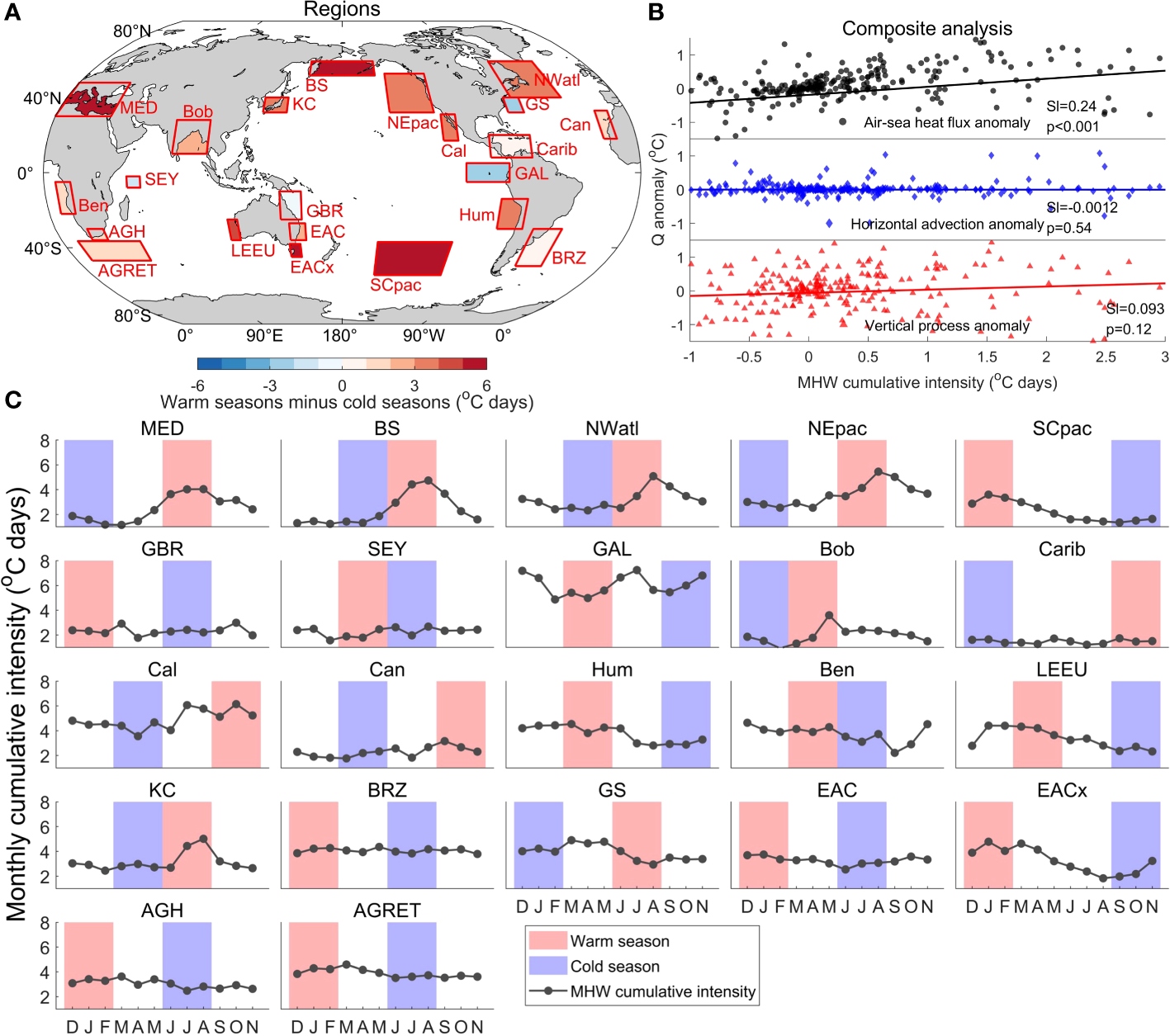
Seasonality of regional MHW cumulative intensity and primary physical processes related to interseasonal difference. Panel (A) shows the interseasonal difference (warm seasons minus cold seasons) in MHW cumulative intensity for 22 typical regions with strong MHWs (Holbrook et al., 2019). Panel (B) shows the result of the composite analysis, which illustrates the correlation between the interseasonal difference in three main physical processes from the heat budget equation and the interseasonal difference in MHW cumulative intensity. Each point indicates an annual interseasonal difference per region. Black dots represent air-sea heat flux anomalies, blue diamonds represent horizontal advection anomalies, and red triangles vertical process anomalies including mainly vertical entrainment and mixing. The Theil-Sen slope (Sl, unit: °C per °C days) and its p-value from the Mann-Kendall test represent the relative correlation among the three processes and corresponding significance. Panel (C) displays the multi-year average of monthly MHW cumulative intensity in the studied regions from 1982 to 2022. The interseasonal difference between warm and cold seasons in MHWs is heightened, particularly in the BS, NEpac, and EACx. Air-sea heat flux is identified as the dominant factor driving the peak of MHWs in the warm season and influencing interseasonal differences.
All daily data required for the heat budget analysis in Section 2.4, including sea surface temperature (SST), net air-sea heat flux, horizontal current velocity, and mixed layer depth used in heat budget analysis are obtained from the Estimating the Circulation and Climate of the Ocean (ECCO) dataset (Forget et al., 2015; ECCO Consortium, 2021; 2024). The ECCO dataset defines the mixed layer depth as the depth at which the temperature difference reaches 0.8°C relative to a 10 m reference depth (Kara et al., 2003). This dataset covers the period from 1992 to 2017.
2.2 MHW definition and characteristics
In this study, we initially subtracted the linear trend of SST to remove the effect of overall warming on MHW detection. We found that the choice of detrending method does not significantly affect the result (Supplementary Figure S1). An MHW at each grid is defined by the detrended SST exceeding the seasonally varying 90th percentile threshold for at least 5 consecutive days (Supplementary Figure S1) (Hobday et al., 2016a). We calculated thresholds using an 11-day window centered on each calendar day across all years to obtain a unique threshold for each day. The seasonally varying threshold allows the identification of anomalously warm events throughout the year, rather than only during the warmest months. The choice of an 11-day window is to ensure a sufficient sample size for percentile estimation. Similarly, climatology is calculated using a multi-year average rather than the 90th percentile. The climatological and threshold baseline period is 30 years from 1982 to 2011. Although the baseline period can affect the magnitude of MHWs, it does not their spatial distribution (Dinesh et al., 2023). By removing the long-term warming, the choice of the specific baseline year becomes less critical. Moreover, gaps of two days or fewer between subsequent events lasting five days or more are regarded as one continuous event.
Based on the detected MHW events, we have defined several characteristics. “MHW days” represents the total number of days MHW events occur per season, which combines the characteristics of MHW frequency and duration (Oliver et al., 2018). “MHW maximum intensity” refers to the highest SST anomaly relative to the climatological mean during a single MHW event, reflecting the most extreme temperature within each season. “MHW cumulative intensity” is the sum of daily SST anomalies in each season, serving as a standardized intensity measure for comparison between seasons. Since we focus on seasonal characteristics and related drivers, we have chosen cumulative intensity as the core standardized indicator in the regional and physical processes analysis across different seasons. We define a season as three months, with four seasons in total: December to February (DJF), March to May (MAM), June to August (JJA), and September to November (SON). We calculate the mean SST for each region in each season, with warm and cold seasons defined based on the maximum and minimum multi-year averaged SST from 1982 to 2022, respectively. The warm and cold seasons vary by region (Figure 1C). Specifically, the warm season is DJF in the Southern Hemisphere high latitudes (i.e., SCpac, GBR, EAC, EACx, AGH, and AGRET), MAM in tropical latitudes (i.e., SEY, GAL, and Bob) and Southern Hemisphere low latitudes (i.e., Hum, Ben, and LEEU), JJA in Northern Hemisphere high latitudes (i.e., MED, BS, NWatl, and NEpac), and SON in Northern Hemisphere low latitudes (i.e., Carib, Cal, and Can). The cold season is DJF (i.e., MED, NEpac, Bob, and Carib) and MAM (i.e., BS, NWatl, Cal, Can, and KC) in Northern Hemisphere, and JJA (i.e., GBR, SEY, Ben, BRZ, EAC, AGH, and AGRET) and SON (i.e., SCpac, GAL, Hum, and LEEU) in Southern hemisphere and tropical latitudes. For 22 typical regions, we compute the cumulative intensity at each grid point for each season, then calculate the area-weighted grid average of these values to determine the regional cumulative intensity.
We modified the MATLAB toolbox (Zhao and Marin, 2019) for MHW detection and matrix calculation. We excluded partial polar regions from the analysis, because the presence of ice cover results in a low SST standard deviation (Huang et al., 2021b), typically less than 0.5°C, making it challenging to accurately identify MHWs in these regions.
2.3 Trend calculation
We examined the temporal trend at each grid and compared their patterns across different regions. The trend was estimated based on the Theil-Sen slope estimator and its statistical significance was tested using the Mann-Kendall test (Sen, 1968; Hussain and Mahmud, 2019). The Theil–Sen trend estimation method is insensitive to outliers and suitable for discontinuous MHW metrics. The Theil-Sen trend and Mann-Kendall test are also used in the following heat budget composite analysis.
2.4 Heat budget equation
The heat budget equation for the mixed layer is a useful tool for attributing changes in MHWs to various physical processes (Stevenson and Niiler, 1983). The mixed layer temperature tendency over a time-varying layer can be mainly controlled by three major processes including horizontal advection, air-sea heat flux, and vertical processes as shown below:
The horizontal advection term, representing the transport of heat by ocean currents is a function of the horizontal velocity fields, calculated by , where u is the horizontal current and is the gradient of SST in the horizontal direction. The air-sea heat flux term is calculated by , where Q is the net surface heat flux composed of four different components including longwave radiation, shortwave radiation, latent heat flux, and sensible heat flux at the ocean surface, Qd is the shortwave radiation penetrating below the mixed layer, h represents the mixed layer depth, ρ is the water density for constant, and Cp is the heat capacity of seawater constant. The residual term is calculated by subtracting the air-sea heat flux and horizontal advection from the temperature tendency, mainly representing vertical entrainment and mixing. For each process, we calculate the anomaly based on the 1992-2017 climatology. Due to the availability of reliable current velocity data with high spatial and temporal resolution since 1992, the time span of our heat budget analysis is limited to the ECCO data coverage from 1992 to 2017. To match ECCO resolution, we re-grid MHWs into a 0.5-degree grid for the heat budget analysis.
2.5 ENSO index
To better understand the influence of ENSO on MHWs across different years, we conducted a comparative analysis among 14 El Niño years, 14 La Niña years, and 13 normal years. El Niño years are identified based on a 3-month moving average of the Niño3.4 index greater than 0.5°C for at least 5 successive months (Santoso et al., 2017). In contrast, La Niña years meet the same criteria, but with an index less than -0.5°C (Santoso et al., 2017). The El Niño years in our study include 1982, 1986, 1987, 1991, 1994, 1997, 2002, 2004, 2006, 2009, 2014, 2015, 2018, and 2019, while the La Niña years include 1983, 1984, 1985, 1988, 1995, 1998, 1999, 2007, 2010, 2011, 2017, 2020, 2021, and 2022. We consider the duration of El Niño and La Niña events often last across years. Therefore, we define the duration of each event from June of the starting year to May of the following year to capture the entire period. This approach is applied to both El Niño and La Niña, as well as to normal years. All calculations for the Niño3.4 index use SST data from the OISST dataset, which is the also dataset used for MHWs analysis.
3 Results
3.1 Seasonal characteristics and trends of global MHWs
Marine heatwaves (MHWs) demonstrate pronounced seasonality in days, maximum intensity, and cumulative intensity (Figure 2). Our analysis from 1982 to 2022 reveals that during June to August (JJA), most mid and high latitudes in the Northern Hemisphere typically experience the highest number of MHW days, with an average of more than 7 days per season (Figures 2B, C). Similarly, parts of the Northeast Pacific Ocean and Northwest Atlantic Ocean peak in MHW days from September to November (SON). Conversely, the Equatorial Eastern Pacific (EEP) and the mid and high latitudes of the Southern Hemisphere experience MHW days mainly in December to February (DJF), also averaging more than 7 days per season. The maximum intensity of MHWs usually peaks in the local summer across most regions, while the cumulative intensity peaks in the summer but extends to autumn in parts of the Northeast Pacific Ocean and Northwest Atlantic Ocean, similar to the pattern observed for MHW days (Figures 2E–I). During these local warm seasons, the global mean of MHW maximum intensity is 3.27°C, with a cumulative intensity of 11.82°C days per season. These values are approximately 1.49 and 1.65 times higher than those recorded in cold seasons, which are 2.20°C and 7.17°C days per season, respectively. In summary, global MHWs consistently exhibit their most severe and prolonged effects during the warm seasons.
Figure 2
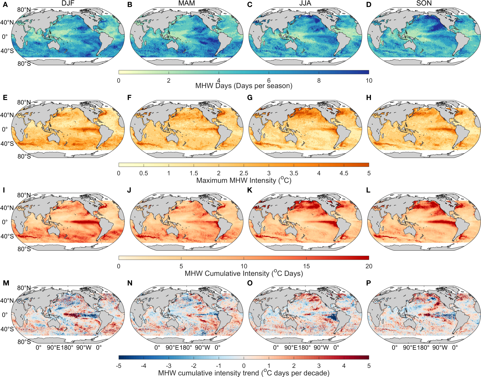
Characteristics of global MHWs in each season from 1982 to 2022. Panels show the seasonal distribution of MHW characteristics: total MHW days (A–D), maximum MHW intensity (E–H), MHW cumulative intensity (I–L), and trends in cumulative intensity using Sen’s slope (M–P), analyzed using the Theil-Sen slope. Red and blue colors in the trend panels (M–P) represent increasing and decreasing cumulative intensity, respectively. Seasons are presented from left to right as December-February (DJF), March-May (MAM), June-August (JJA), and September-November (SON). The results reveal a pronounced seasonality in MHWs, typically reaching their peak intensity during the local warm seasons in most regions. In addition, they also display large spatial heterogeneity, with areas experiencing high intensity showing a significant increasing trend.
In addition to seasonality, the global observation of MHW days and intensity also exhibit an uneven spatial distribution. Certain regions experience longer and high-intense MHWs, including the northeast and northwest Pacific, EEP, northwest and southwest Atlantic, Arctic subpolar regions, eastern Australia, and the Southern Ocean south of Africa (Figure 2). In these regions, the cumulative intensity during warm seasons exceeds 21.85°C days per season, which is more than double of that in other regions. While the spatial distribution of maximum and cumulative intensity of MHWs is consistent within each season, the spatial variations are larger during warm seasons due to the stronger intensity in these specific areas during warm seasons.
MHWs in large areas of the globe are associated with high SST variability, indicating that regions with the most intense MHWs generally correspond to regions with large SST fluctuations. The relationship is reflected in the Pearson correlation coefficient between seasonal mean cumulative intensity and SST variability, which is significant (p<0.001) in JJA (0.76), DJF (0.70), SON (0.66), and March to May (MAM, 0.59) (Supplementary Figure S2). This implies that regions with high SST variability are more likely to experience large-intensity MHWs in all seasons, as larger SST variances lead to more extreme conditions (Supplementary Figure S2).
Globally, MHWs are exhibiting an increasing trend across all seasons, with areas already experiencing stronger MHWs demonstrating an even more pronounced trend. From 1982 to 2022, the global MHW cumulative intensity increased significantly, peaking in JJA with an increase rate of 1.35°C days per season per decade (p<0.01). The increasing cumulative intensity trend holds even after accounting for long-term warming (Supplementary Figure S3). In all seasons, more than half of the world’s oceans show increasing MHW cumulative intensity, with the largest increase ratio in JJA at 58.9%, and 11.1% of these areas showed a statistically significant increase (p<0.05) (Figure 2N). The most significant increases predominantly occurred in regions with high-intensity MHWs, with an increase of more than 3.47°C days per decade during the last 40 years. Despite the overall positive global trend of MHWs, MHWs in EEP show a notable declining trend in contrast to the central equatorial Pacific across all seasons. Especially in DJF, the spatial pattern resembles that of El Niño events. This observation aligns with the studies showing a faster growth of central El Niño events while the EEP suffers more La Niña periods (Shin et al., 2022).
3.2 Seasonality and interseasonal difference in MHWs by region
Large interseasonal differences in MHWs between warm and cold seasons are observed in mid and high latitude and boundary current regions, while tropical latitudes exhibit a small difference except Galapagos Islands (GAL) and Bay of Bengal (Bob) (Figure 1). High latitude regions, such as the Mediterranean Sea (MED), Bering Sea (BS), Northwest Atlantic Ocean (NWatl), Northeast Pacific Ocean (NEpac), and South-Central Pacific Ocean (SCpac), exhibit MHW cumulative intensity that is greater than 3°C days per season higher in the warm season compared to the cold season. Similarly, in the eastern and western boundary current areas, the interseasonal difference increases with latitude. Particularly, for the California Current (Cal), Humboldt Current (Hum), Leeuwin Current (LEEU), Kuroshio-Oyashio (KC), and EAC Extension (EACx), the interseasonal difference also surpasses 3°C days per season. Conversely, tropical latitudes show minimal interseasonal differences. Notably, the difference in the GAL and Bob is larger compared to other tropical regions such as the Great Barrier Reef (GBR), Seychelles Islands (SEY), and Caribbean Sea (Carib), likely due to the stronger influence of El Niño-Southern Oscillation (ENSO) in GAL and Bob, as discussed further in Section 3.3 (Holbrook et al., 2019; Lin et al., 2023).
The interseasonal difference in MHWs is primarily driven by substantial air-sea heat flux anomalies, according to our composite analysis (Figure 1B). A robust positive correlation is observed between the interseasonal difference in air-sea heat flux anomalies and MHWs (p<0.001) (Figure 1B). Consequently, regions with a large interseasonal difference in air-sea heat flux anomaly demonstrates a more pronounced interseasonal difference in MHWs. The correlations between horizontal advection and vertical process are not statistically significant. While previous research has suggested that ocean advection is the primary driver for the development and decline of MHWs in the eastern and western boundary current areas, as well as for the formation of the deepest MHWs (Zhang et al., 2021, 2023; Bian et al., 2024), our research shows that air-sea heat flux dominates its interseasonal difference. We found that interseasonal difference in MHWs shows little correlation with ocean advection and vertical processes (Figure 1B).
Over the past four decades, the interseasonal difference of MHWs has increased in most regions (Figure 3A). The trend of MHW cumulative intensity in the warm season is significantly increasing, while the trend of MHW cumulative intensity in the cold season is weak in most regions. This combination of a strong increasing trend in the warm season and a weak trend in the cold season leads to an increasing interseasonal difference in MHWs. In the BS, NWatl, NEpac, and EACx, the significant increase in MHW cumulative intensity in the warm season plays a more crucial role in the trend in interseasonal difference (Figure 3A). In the Brazil-Malvinas Confluence (BRZ) and Agulhas Retroflection (AGRET), MHWs have intensified in both warm and cold seasons, while the interseasonal difference remains relatively unchanged.
Figure 3
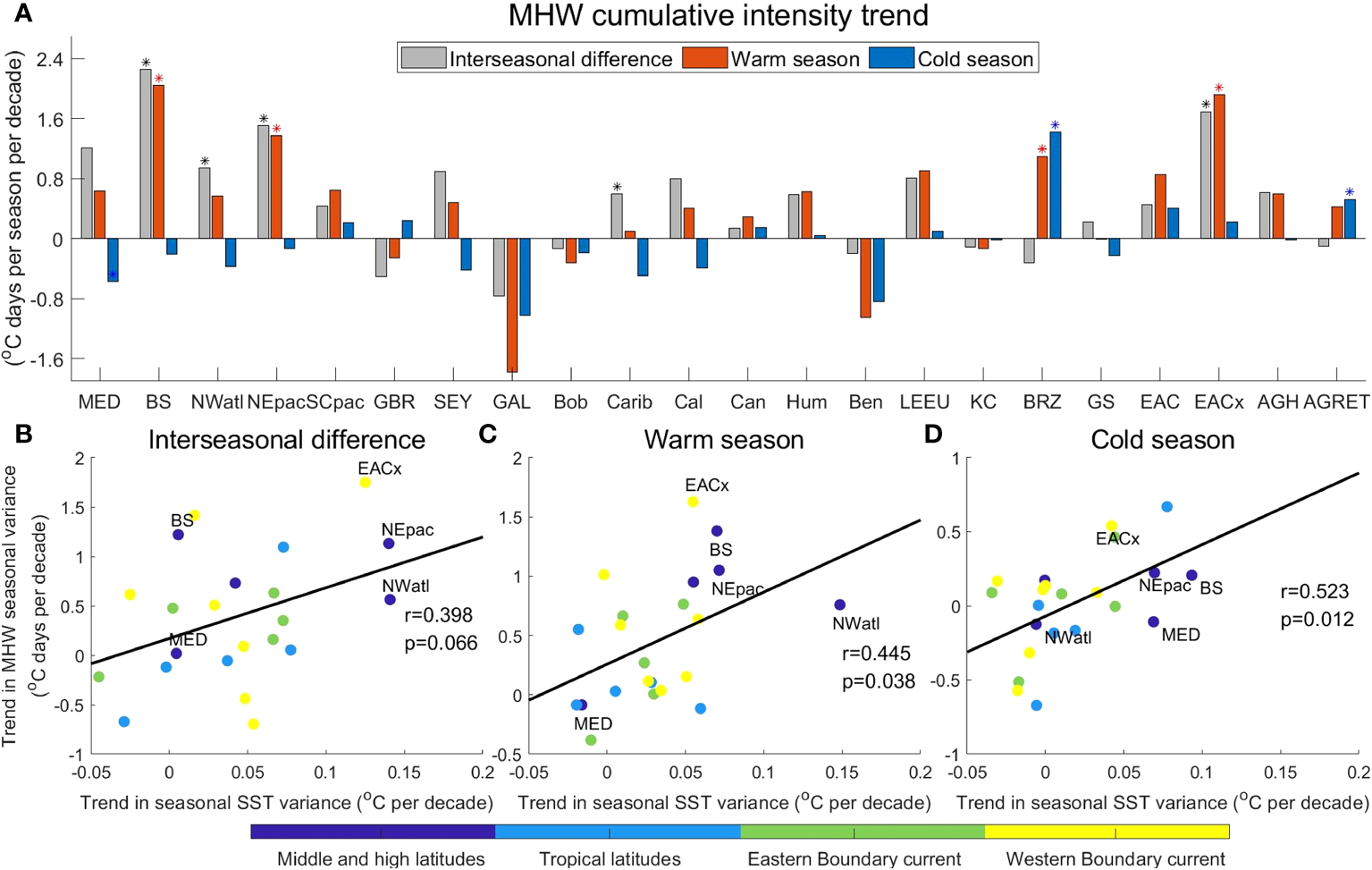
Trend in the interseasonal difference of MHW cumulative intensity. Panel (A) presents the linear trend of interseasonal difference in MHW cumulative intensity (grey bars) and MHW trend in warm seasons (red bars) and cold seasons (blue bars), respectively. The asterisk (*) indicates the trend is significant at a 95% confidence level. Panels (B–D) show the correlation between the trend of MHWs and the trend of SST variance in the interseasonal difference, warm season, and cold season, respectively. The results reveal the enhanced interseasonal difference in MHWs is strongly correlated with the increasing trend in SST variance, particularly in warm seasons.
Furthermore, the increasing interseasonal difference in MHWs is strongly correlated with the increasing interseasonal difference in SST variance. The trend of interseasonal difference in MHWs shows a positive correlation with the trend of interseasonal SST variance (r=0.398, p=0.066) (Figures 3B–D). Specifically, the significantly positive relationship is strong in both warm (r=0.445, p<0.05) and cold seasons (r=0.523, p<0.05), respectively. This suggests that the pronounced interseasonal difference in MHWs, particularly in areas such as EACx, NEPac, and NWatl, is significantly influenced by the substantial increase in SST variance.
3.3 The effect of ENSO on MHWs
When comparing MHWs after removing the linear Niño3.4 index with those not removed, it is evident that ENSO significantly exacerbates the MHW cumulative intensity in the tropical regions (Figure 4). Specifically, after removing the Niño3.4 index, MHW cumulative intensity in the Eastern Equatorial Pacific (EEP) decreases to 6.14°C days per season, a significant 53% reduction compared to the 12.96°C days before the removal of the Niño3.4 index. During El Niño years, the impact of ENSO becomes even more pronounced on MHWs in the EEP (Figure 4A). These El Niño periods are characterized by weakened trade winds, leading to a shallower mixed layer and reduced cold oceanic upwelling, which can amplify sea surface warming (Newman et al., 2018). During La Niña period, ENSO has no significant impact on MHWs in the EEP (Figure 4B). Meanwhile, ENSO has almost no persistent impact that lasts into normal years (Figure 4C). In the Western Equatorial Indian Ocean, we observe an average decrease of 0.42°C days per season of MHW cumulative intensity after removing the Niño3.4 index, which further decreased by 2.80°C days during El Niño years. Conversely, during La Niña years, the effects of inhibiting MHWs in the Indian Ocean are relatively small and not statistically significant (Figure 4B).
Figure 4
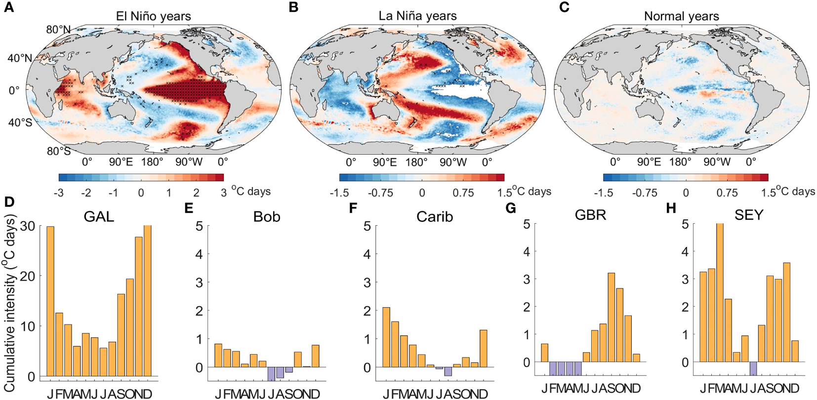
The effects of ENSO on MHWs. The monthly mean cumulative intensity (°C days) of MHWs is calculated by detrended SST, subtracting MHWs calculated from SSTs that are processed by both detrending and removing linear Niño3.4 index. Panels (A–C) show a synthetic average of different typical years: (A) El Niño years, (B) La Niña years, and (C) normal years, as detailed in the methods. Black dots indicate a statistically significant effect of ENSO on MHWs, as determined by a t-test with p-values less than 0.05. Panels (D–H) show the effects of ENSO in different seasons in equatorial regions: Galápagos (GAL), Bay of Bengal (Bob), Caribbean Sea (Carib), Great Barrier Reef (GBR), and Seychelles (SEY). Yellow bars indicate a positive effect of ENSO on MHWs, while purple bars mean inhibition. ENSO significantly exacerbates MHW cumulative intensity in the equatorial regions, especially during winter in El Niño years, serving as the primary driver for the strong MHWs from December to February.
The effects of ENSO are most pronounced from December to February, with notable interseasonal variations observed in the GAL, Bob, Carib, GBR, and SEY (Figures 4D–H and Supplementary Figure S4). In the GAL, ENSO is the dominant factor accounting for the interseasonal influence in MHWs since the interseasonal influence of ENSO is consistent with the seasonal cycle of MHWs (Figure 4D). Furthermore, in the Indian Ocean (i.e., SEY and Bob), two peaks of MHW in DJF and MAM are likely related to ENSO (Figures 4E, H). One peak is influenced by the contemporaneous impact of ENSO, while the other is affected by the Indian Ocean Dipole lagging behind ENSO. The consistent results from regional studies (i.e., Western equatorial Indian Ocean and North Indian Ocean) confirm that the interseasonal variations in MHWs in the Indian Ocean are influenced by ENSO (Xie et al., 2016; Qi et al., 2022).
4 Discussions and conclusions
Our study enhances the understanding of the seasonal characteristics of marine heatwaves (MHWs) in different regions and the dominant physical processes involved. We found that air-sea heat flux is a key factor explaining the peak cumulative intensity of MHWs in warm seasons for most regions. The cumulative intensity reflects the most ecological impacts, combining both MHW duration and intensity. At the same cumulative intensity, more frequent but milder MHW days may have different impacts compared to fewer but more intense MHW days, depending on the affected species and communities. Furthermore, the increasing interseasonal difference of MHWs, mainly dominated by the increasing trend in warm season MHWs, is strongly correlated with the increasing interseasonal SST variance. Strong SST variations may be attributed to anomalous advection caused by the fast, narrow, and unstable boundary current, as seen in western boundary currents. These currents are marked by enhanced horizontal heat advection and high eddy kinetic energy (Ma et al., 2016; Elzahaby et al., 2021). In the equatorial regions, ENSO exacerbates MHWs in the Eastern Equatorial Pacific, especially during El Niño winters, and drives two peak MHWs in winter and subsequent spring in the Western Equatorial Indian Ocean. Since we synthesize different typical years to distinguish the effects of different phases of ENSO in various seasons on MHWs, specific processes associated with individual events are omitted. We propose further studies focus on the continuous tracking of the effects of a single large El Niño or La Niña event on MHWs. Simultaneously, whether El Niño events should be included in MHWs is also a controversial issue. It is necessary to refine a reasonable definition of MHWs based on the relationship between ENSO and MHWs as we discussed above.
In our methodology for detecting MHWs, we account for a long-term warming trend to ensure that our identification of MHWs is not influenced by the overall increase in global average SST. Compared to using raw time series to directly identify MHWs, our results for characteristics including MHW days, maximum intensity, and cumulative intensity are more conservative than using raw SST (37%, 26%, and 52% less) (Supplementary Figure S5). The strong correlation between MHW cumulative intensity and SST variability supports our detrend MHWs detection method, which effectively removes the long-term warming while retaining the changes in SST variability. Although the long-term warming is subtracted, the increasing rate remains significant in most oceans, and the high-intensity regions remain extreme. This conservative MHW detection helps rationally assess the impact of MHW on ecosystems and highlights the extreme regions, emphasizing the urgent need for more attention. Moreover, we recognize the reasonability of using a fixed baseline for studies focusing on the slow adaption and immobile species, such as corals (Smith et al., 2023).
We recognize the complexity of attributing MHWs to specific physical processes due to the limitations of our approach, which does not differentiate between short-term and long-term MHWs. Some studies adopt non-uniform identification methods such as high-pass filtering to obtain the time range of the physical processes corresponding to the wind (Cooley et al., 2022). The detection method depends on the physical processes they are concerned about. Our method aims for universality in analyzing global MHWs across different oceans. However, there needs to be a clear distinction between high- and low-frequency MHWs, which will support comprehensive studies on global physical processes.
In conclusion, our detecting approach provides valuable insights into the seasonal characteristics of MHWs. These insights not only provide a more conservative MHW estimation but also pave the way for better-informed policies and a more thorough understanding of MHWs’ economic and ecological impacts. This work contributes to making accurate future models and the development of reasonable environmental protection policies.
Statements
Data availability statement
Data used in the analysis were obtained from publicly available sources as cited. OISST V2.1 sea surface temperature data was obtained from https://www.ncei.noaa.gov/data/sea-surface-temperature-optimum-interpolation/v2.1/access/avhrr/. ECCOv4r4 was provided by NASA/JPL from http://ecco-group.org/products-ECCO-V4r4.htm.
Author contributions
YW: Writing – review & editing, Writing – original draft, Visualization, Data curation, Conceptualization. YZ: Writing – review & editing, Writing – original draft, Supervision, Funding acquisition, Conceptualization.
Funding
The author(s) declare financial support was received for the research, authorship, and/or publication of this article. This research was supported by the National Natural Science Foundation of China (42341201, 42276201) and the Oceanic Interdisciplinary Program of Shanghai Jiao Tong University (SL2022PT204).
Acknowledgments
We thank the National Oceanic and Atmospheric Administration (NOAA) for providing the production, availability, and maintenance of NOAA Optimum interpolation 0.25° daily sea surface temperature analysis. We also thank NASA’s ECCO project for providing the sea surface temperature (SST), net air-sea heat flux, horizontal current velocity, and mixed layer depth data.
Conflict of interest
The authors declare that the research was conducted in the absence of any commercial or financial relationships that could be construed as a potential conflict of interest.
Publisher’s note
All claims expressed in this article are solely those of the authors and do not necessarily represent those of their affiliated organizations, or those of the publisher, the editors and the reviewers. Any product that may be evaluated in this article, or claim that may be made by its manufacturer, is not guaranteed or endorsed by the publisher.
Supplementary material
The Supplementary Material for this article can be found online at: https://www.frontiersin.org/articles/10.3389/fmars.2024.1406416/full#supplementary-material
References
1
Amaya D. J. Jacox M. G. Fewings M. R. Saba V. S. Stuecker M. F. Rykaczewski R. R. et al . (2023). Marine heatwaves need clear definitions so coastal communities can adapt. Nature616, 29–32. doi: 10.1038/d41586-023-00924-2
2
Atkinson J. King N. G. Wilmes S. B. Moore P. J. (2020). Summer and winter marine heatwaves favor an invasive over native seaweeds. J. Phycol.56, 1591–1600. doi: 10.1111/jpy.13051
3
Banzon V. Smith T. M. Chin T. M. Liu C. Hankins W. (2016). A long-term record of blended satellite and in situ sea-surface temperature for climate monitoring, modeling and environmental studies. Earth Syst. Sci. Data8, 165–176. doi: 10.5194/essd-8-165-2016
4
Benthuysen J. A. Oliver E. C. J. Feng M. Marshall A. G. (2018). Extreme marine warming across tropical Australia during austral summer 2015–2016. J. Geophys. Res.: Oceans123, 1301–1326. doi: 10.1002/2017jc013326
5
Bian C. Jing Z. Wang H. Wu L. (2024). Scale-dependent drivers of marine heatwaves globally. Geophys. Res. Lett.51, e2023GL107306. doi: 10.1029/2023gl107306
6
Cavole L. Demko A. Diner R. Giddings A. Koester I. Pagniello C. et al . (2016). Biological impacts of the 2013–2015 warm-water anomaly in the northeast Pacific: winners, losers, and the future. Oceanography29, 273–285. doi: 10.5670/oceanog.2016.32
7
Cheung W. W. L. Frolicher T. L. (2020). Marine heatwaves exacerbate climate change impacts for fisheries in the northeast Pacific. Sci. Rep.10, 6678. doi: 10.1038/s41598-020-63650-z
8
Chiswell S. M. (2022). Global trends in marine heatwaves and cold spells: the impacts of fixed versus changing baselines. J. Geophys. Res.: Oceans127, e2022JC018757. doi: 10.1029/2022jc018757
9
Cooley K. M. Fewings M. R. Lerczak J. A. O’Neill L. W. Brown K. S. (2022). Role of sea surface physical processes in mixed-layer temperature changes during summer marine heat waves in the Chile-Peru current system. J. Geophys. Res.: Oceans127, e2021JC018338. doi: 10.1029/2021JC018338
10
Curnock M. I. Marshall N. A. Thiault L. Heron S. F. Hoey J. Williams G. et al . (2019). Shifts in tourists’ sentiments and climate risk perceptions following mass coral bleaching of the Great Barrier Reef. Nat. Climate Change9, 535–541. doi: 10.1038/s41558-019-0504-y
11
Darmaraki S. Somot S. Sevault F. Nabat P. Cabos Narvaez W. D. Cavicchia L. et al . (2019). Future evolution of marine heatwaves in the Mediterranean Sea. Climate Dyn.53, 1371–1392. doi: 10.1007/s00382-019-04661-z
12
Dinesh A. S. Mishra A. K. Dubey A. K. Kumari S. Anand A. (2023). Comparative changes in seasonal marine heatwaves and cold spells over the Tropical Indian Ocean during recent decades and disentangling the drivers of highly intense events. Int. J. Climatol.43, 7428–7446. doi: 10.1002/joc.8272
13
ECCO Consortium F. ,. I. Wang O. Fenty I. Forget G. Heimbach P. Ponte R. M. (2021). (2021, February 10). Synopsis of the ECCO central production global ocean and sea-ice state estimate (Version 4 release 4). doi: 10.5281/zenodo.4533349
14
ECCO Consortium F. ,. I. Wang O. Fenty I. Forget G. Heimbach P. Ponte R. M. (2024) ECCO Central Estimate (Version 4 Release 4). Available online at: http://ecco-group.org/products-ECCO-V4r4.htm.
15
Elzahaby Y. Schaeffer A. Roughan M. Delaux S. (2021). Oceanic circulation drives the deepest and longest marine heatwaves in the east Australian current system. Geophys. Res. Lett.48, e2021GL094785. doi: 10.1029/2021gl094785
16
Ferriss B. E. Marcinek D. J. Ayres D. Borchert J. Lefebvre K. A. (2017). Acute and chronic dietary exposure to domoic acid in recreational harvesters: A survey of shellfish consumption behavior. Environ. Int.101, 70–79. doi: 10.1016/j.envint.2017.01.006
17
Forget G. Campin J. M. Heimbach P. Hill C. N. Ponte R. M. Wunsch C. (2015). ECCO version 4: an integrated framework for non-linear inverse modeling and global ocean state estimation. Geosci. Model. Dev.8, 3071–3104. doi: 10.5194/gmd-8-3071-2015
18
Frolicher T. L. Fischer E. M. Gruber N. (2018). Marine heatwaves under global warming. Nature560, 360–364. doi: 10.1038/s41586-018-0383-9
19
Frolicher T. L. Laufkotter C. (2018). Emerging risks from marine heat waves. Nat. Commun.9, 650. doi: 10.1038/s41467-018-03163-6
20
Garcia-Soto C. Cheng L. Caesar L. Schmidtko S. Jewett E. B. Cheripka A. et al . (2021). An overview of ocean climate change indicators: sea surface temperature, ocean heat content, ocean pH, dissolved oxygen concentration, Arctic sea ice extent, thickness and volume, sea level and strength of the AMOC (Atlantic meridional overturning circulation). Front. Mar. Sci.8. doi: 10.3389/fmars.2021.642372
21
Garrabou J. Gomez-Gras D. Medrano A. Cerrano C. Ponti M. Schlegel R. et al . (2022). Marine heatwaves drive recurrent mass mortalities in the Mediterranean Sea. Global Change Biol.28, 5708–5725. doi: 10.1111/gcb.16301
22
Hobday A. J. Alexander L. V. Perkins S. E. Smale D. A. Straub S. C. Oliver E. C. J. et al . (2016a). A hierarchical approach to defining marine heatwaves. Prog. Oceanogr.141, 227–238. doi: 10.1016/j.pocean.2015.12.014
23
Hobday A. J. Spillman C. M. Paige Eveson J. Hartog J. R. (2016b). Seasonal forecasting for decision support in marine fisheries and aquaculture. Fisheries Oceanogr.25, 45–56. doi: 10.1111/fog.12083
24
Holbrook N. J. Claar D. C. Hobday A. J. McInnes K. L. Oliver E. C. J. Gupta A. S et al . (2020). ENSO-Driven Ocean Extremes and Their Ecosystem Impacts. In El Niño Southern Oscillation in a Changing Climate (eds McPhadenM. J.SantosoA.CaiW). doi: 10.1002/9781119548164.ch18
25
Holbrook N. J. Scannell H. A. Sen Gupta A. Benthuysen J. A. Feng M. Oliver E. C. J. et al . (2019). A global assessment of marine heatwaves and their drivers. Nat. Commun.10, 2624. doi: 10.1038/s41467-019-10206-z
26
Huang B. Liu C. Banzon V. Freeman E. Graham G. Hankins B. et al . (2021a). Improvements of the daily optimum interpolation sea surface temperature (DOISST) version 2.1. J. Climate34, 2923–2939. doi: 10.1175/jcli-d-20-0166.1
27
Huang B. Wang Z. Yin X. Arguez A. Graham G. Liu C. et al . (2021b). Prolonged marine heatwaves in the arctic: 1982–2020. Geophys. Res. Lett.48, e2021GL095590. doi: 10.1029/2021gl095590
28
Hughes T. P. Anderson K. D. Connolly S. R. Heron S. F. Kerry J. T. Lough J. M. et al . (2018). Spatial and temporal patterns of mass bleaching of corals in the Anthropocene. Science359, 80–83. doi: 10.1126/science.aan8048
29
Hussain M. Mahmud I. (2019). pyMannKendall: a python package for non parametric Mann Kendall family of trend tests. J. Open Source Softw.4, 1556.
30
Jacox M. G. (2019). Marine heatwaves in a changing climate. Nature571, 485–487. doi: 10.1038/d41586-019-02196-1
31
Jacox M. G. Alexander M. A. Amaya D. Becker E. Bograd S. J. Brodie S. et al . (2022). Global seasonal forecasts of marine heatwaves. Nature604, 486–490. doi: 10.1038/s41586-022-04573-9
32
Kajtar J. B. Bachman S. D. Holbrook N. J. Pilo G. S. (2022). Drivers, dynamics, and persistence of the 2017/2018 Tasman sea marine heatwave. J. Geophys. Res.: Oceans127, e2022JC018931. doi: 10.1029/2022jc018931
33
Kara A. B. Rochford P. A. Hurlburt H. E. (2003). Mixed layer depth variability over the global ocean. J. Geophys. Res.: Oceans108, 3079. doi: 10.1029/2000jc000736
34
Koul V. Brune S. Akimova A. Düsterhus A. Pieper P. Hövel L. et al . (2023). Seasonal prediction of Arabian sea marine heatwaves. Geophys. Res. Lett.50, e2023GL103975. doi: 10.1029/2023gl103975
35
Kumar P. Dinesh A. S. Mishra A. K. Pandey L. K. Sein D. V. Ryabchenko V. A. (2024). Marine heatwaves intensification, expansion and departure into the permanent state over the Tropical Indian Ocean: A regional earth system model assessment. Dyn. Atmos. Oceans105, 101408. doi: 10.1016/j.dynatmoce.2023.101408
36
Lin X. Qiu Y. Wang J. Teng H. Ni X. Liang K. (2023). Seasonal diversity of el niño-induced marine heatwave increases in the bay of Bengal. Geophys. Res. Lett.50, e2022GL100807. doi: 10.1029/2022gl100807
37
Ling S. D. Johnson C. R. Ridgway K. Hobday A. J. Haddon M. (2009). Climate-driven range extension of a sea urchin: inferring future trends by analysis of recent population dynamics. Global Change Biol.15, 719–731. doi: 10.1111/j.1365-2486.2008.01734.x
38
Ma X. Jing Z. Chang P. Liu X. Montuoro R. Small R. J. et al . (2016). Western boundary currents regulated by interaction between ocean eddies and the atmosphere. Nature535, 533–537. doi: 10.1038/nature18640
39
McRae C. J. Keshavmurthy S. Meng P.-J. Rosset S. L. Huang W.-B. Chen C. A. et al . (2022). Variable responses to chronic and acute elevated temperature of three coral species from reefs with distinct thermal regimes. Mar. Biol.169, 97. doi: 10.1007/s00227-022-04071-6
40
Newman M. Wittenberg A. T. Cheng L. Compo G. P. Smith C. A. (2018). The extreme 2015/16 el niño, in the context of historical climate variability and change. Bull. Am. Meteorol. Soc.99, S16–S20. doi: 10.1175/bams-d-17-0116.1
41
Oliver E. C. J. Benthuysen J. A. Darmaraki S. Donat M. G. Hobday A. J. Holbrook N. J. et al . (2021). Marine heatwaves. Annu. Rev. Mar. Sci.13, 313–342. doi: 10.1146/annurev-marine-032720-095144
42
Oliver E. C. J. Donat M. G. Burrows M. T. Moore P. J. Smale D. A. Alexander L. V. et al . (2018). Longer and more frequent marine heatwaves over the past century. Nat. Commun.9, 1324. doi: 10.1038/s41467-018-03732-9
43
Pershing A. J. Alexander M. A. Hernandez C. M. Kerr L. A. Le Bris A. Mills K. E. et al . (2015). Slow adaptation in the face of rapid warming leads to collapse of the Gulf of Maine cod fishery. Science350, 809–812. doi: 10.1126/science.aac9819
44
Piatt J. F. Parrish J. K. Renner H. M. Schoen S. K. Jones T. T. Arimitsu M. L. et al . (2020). Extreme mortality and reproductive failure of common murres resulting from the northeast Pacific marine heatwave of 2014-2016. PloS One15, e0226087. doi: 10.1371/journal.pone.0226087
45
Qi R. Zhang Y. Du Y. Feng M. (2022). Characteristics and drivers of marine heatwaves in the western equatorial Indian ocean. J. Geophys. Res.: Oceans127, e2022JC018732. doi: 10.1029/2022jc018732
46
Rogers-Bennett L. Catton C. A. (2019). Marine heat wave and multiple stressors tip bull kelp forest to sea urchin barrens. Sci. Rep.9, 15050. doi: 10.1038/s41598-019-51114-y
47
Rosselló P. Pascual A. Combes V. (2023). Assessing marine heat waves in the Mediterranean Sea: a comparison of fixed and moving baseline methods. Front. Mar. Sci.10. doi: 10.3389/fmars.2023.1168368
48
Santoso A. McPhaden M. J. Cai W. (2017). The defining characteristics of ENSO extremes and the strong 2015/2016 el niño. Rev. Geophys.55, 1079–1129. doi: 10.1002/2017rg000560
49
Schlax M. G. Casey K. S. Chelton D. B. Liu C. Smith T. M. Reynolds R. W. (2007). Daily high-resolution-blended analyses for sea surface temperature. J. Climate20, 5473–5496. doi: 10.1175/2007jcli1824.1
50
Sen P. K. (1968). Estimates of the regression coefficient based on Kendall’s Tau. J. Am. Stat. Assoc.63, 1379–1389. doi: 10.1080/01621459.1968.10480934
51
Sen Gupta A. Thomsen M. Benthuysen J. A. Hobday A. J. Oliver E. Alexander L. V. et al . (2020). Drivers and impacts of the most extreme marine heatwaves events. Sci. Rep.10, 19359. doi: 10.1038/s41598-020-75445-3
52
Shin N.-Y. Kug J.-S. Stuecker M. F. Jin F.-F. Timmermann A. Kim G.-I. (2022). More frequent central Pacific El Niño and stronger eastern pacific El Niño in a warmer climate. NPJ Climate Atmos. Sci.5, 101. doi: 10.1038/s41612-022-00324-9
53
Simon A. Plecha S. M. Russo A. Teles-MaChado A. Donat M. G. Auger P.-A. et al . (2022). Hot and cold marine extreme events in the Mediterranean over the period 1982-2021. Front. Mar. Sci.9. doi: 10.3389/fmars.2022.892201
54
Smale D. A. Wernberg T. Oliver E. C. J. Thomsen M. Harvey B. P. Straub S. C. et al . (2019). Marine heatwaves threaten global biodiversity and the provision of ecosystem services. Nat. Climate Change9, 306–312. doi: 10.1038/s41558-019-0412-1
55
Smith K. E. Burrows M. T. Hobday A. J. King N. G. Moore P. J. Sen Gupta A. et al . (2023). Biological impacts of marine heatwaves. Annu. Rev. Mar. Sci.15, 119–145. doi: 10.1146/annurev-marine-032122-121437
56
Smith K. E. Burrows M. T. Hobday A. J. Sen Gupta A. Moore P. J. Thomsen M. et al . (2021). Socioeconomic impacts of marine heatwaves: Global issues and opportunities. Science374, eabj3593. doi: 10.1126/science.abj3593
57
Spillman C. M. Smith G. A. Hobday A. J. Hartog J. R. (2021). Onset and decline rates of marine heatwaves: global trends, seasonal forecasts and marine management. Front. Climate3. doi: 10.3389/fclim.2021.801217
58
Stevenson J. W. Niiler P. P. (1983). Upper ocean heat budget during the Hawaii-to-Tahiti shuttle experiment. J. Phys. Oceanogr.13, 1894–1907. doi: 10.1175/1520-0485(1983)013<1894:Uohbdt>2.0.Co;2
59
Tan H. Cai R. Wu R. (2022). Summer marine heatwaves in the South China Sea: Trend, variability and possible causes. Adv. Climate Change Res.13, 323–332. doi: 10.1016/j.accre.2022.04.003
60
Thoral F. Montie S. Thomsen M. S. Tait L. W. Pinkerton M. H. Schiel D. R. (2022). Unravelling seasonal trends in coastal marine heatwave metrics across global biogeographical realms. Sci. Rep.12, 7740. doi: 10.1038/s41598-022-11908-z
61
von Kietzell A. Schurer A. Hegerl G. C. (2022). Marine heatwaves in global sea surface temperature records since 1850. Environ. Res. Lett.17, 084027. doi: 10.1088/1748-9326/ac81db
62
Wang W. McPhaden M. J. (1999). The surface-layer heat balance in the equatorial Pacific Ocean. Part I: mean seasonal cycle*. J. Phys. Oceanogr.29, 1812–1831. doi: 10.1175/1520-0485(1999)029<1812:Tslhbi>2.0.Co;2
63
Xie S.-P. Kosaka Y. Du Y. Hu K. Chowdary J. S. Huang G. (2016). Indo-western Pacific ocean capacitor and coherent climate anomalies in post-ENSO summer: A review. Adv. Atmos. Sci.33, 411–432. doi: 10.1007/s00376-015-5192-6
64
Xu T. Newman M. Capotondi A. Stevenson S. Di Lorenzo E. Alexander M. A. (2022). An increase in marine heatwaves without significant changes in surface ocean temperature variability. Nat. Commun.13, 7396. doi: 10.1038/s41467-022-34934-x
65
Yao Y. Wang C. (2021). Variations in summer marine heatwaves in the South China Sea. J. Geophys. Res.: Oceans126, e2021JC017792. doi: 10.1029/2021jc017792
66
Yao Y. Wang C. Fu Y. (2022). Global marine heatwaves and cold-spells in present climate to future projections. Earth’s Future10. doi: 10.1029/2022ef002787
67
Zhang Y. Du Y. Feng M. Hobday A. J. (2023). Vertical structures of marine heatwaves. Nat. Commun.14, 6483. doi: 10.1038/s41467-023-42219-0
68
Zhang Y. Du Y. Feng M. Hu S. (2021). Long-lasting marine heatwaves instigated by ocean planetary waves in the tropical Indian ocean during 2015–2016 and 2019–2020. Geophys. Res. Lett.48, e2021GL095350. doi: 10.1029/2021gl095350
69
Zhao Z. Marin M. (2019). A MATLAB toolbox to detect and analyze marine heatwaves. J. Open Source Softw.4, 1124. doi: 10.21105/joss.01124
Summary
Keywords
marine heatwaves, seasonality, air-sea heat flux, interseasonal difference, ENSO
Citation
Wang Y and Zhou Y (2024) Seasonal dynamics of global marine heatwaves over the last four decades. Front. Mar. Sci. 11:1406416. doi: 10.3389/fmars.2024.1406416
Received
25 March 2024
Accepted
29 April 2024
Published
04 June 2024
Volume
11 - 2024
Edited by
Toru Miyama, Japan Agency for Marine-Earth Science and Technology, Japan
Reviewed by
Alok Kumar Mishra, Agricultural Research Organization (ARO), Israel
François Thoral, University of Waikato, New Zealand
Updates
Copyright
© 2024 Wang and Zhou.
This is an open-access article distributed under the terms of the Creative Commons Attribution License (CC BY). The use, distribution or reproduction in other forums is permitted, provided the original author(s) and the copyright owner(s) are credited and that the original publication in this journal is cited, in accordance with accepted academic practice. No use, distribution or reproduction is permitted which does not comply with these terms.
*Correspondence: Yuntao Zhou, ytzhou@sjtu.edu.cn
Disclaimer
All claims expressed in this article are solely those of the authors and do not necessarily represent those of their affiliated organizations, or those of the publisher, the editors and the reviewers. Any product that may be evaluated in this article or claim that may be made by its manufacturer is not guaranteed or endorsed by the publisher.