Fine-scale hydrodynamics around St. John, U.S. Virgin Islands. Part II: variability in residence time in coastal bays

Coastal currents can vary dramatically in space and time, influencing advection and residence time of larvae, nutrients and contaminants in coastal environments. However, spatial and temporal variabilities of the residence time of these materials in coastal environments, such as coastal bays, are rarely quantified in ecological applications. Here, we use a particle tracking model built on top of the high-resolution hydrodynamic model described in Part 1 to simulate the dispersal of particles released in coastal bays around a key and model island study site, St. John, USVI without considering the impact of surface waves. Motivated to provide information for future coral and fish larval dispersal and contaminant spreading studies, this first step of the study toward understanding fine-scale dispersal variability in coastal bays aimed to characterize the cross-bay variability of particle residence time in the bays. Both three-dimensionally distributed (3D) and surface-trapped (surface) particles are considered. Model simulations show pronounced influences of winds, intruding river plumes, and bay orientation on the residence time. The residence times of 3D particles in many of the bays exhibit a clear seasonality, correlating with water column stratification and patterns of the bay-shelf exchange flow. When the water column is well-mixed, the exchange flow is laterally sheared, allowing a significant portion of exported 3D particles to re-enter the bays, resulting in high residence times. During stratified seasons, due to wind forcing or intruding river plumes, the exchange flows are vertically sheared, reducing the chance of 3D particles returning to the bays and their residence time in the bays. For a westward-facing bay with the axis aligned the wind, persistent wind-driven surface flows carry surface particles out of the bays quickly, resulting in a low residence time in the bay; when the bay axis is misaligned with the wind, winds can trap surface particles on the west coast in the bay and dramatically increase their residence time. The strong temporal and inter-bay variation in the duration of particles staying in the bays, and their likely role in larval and contaminant dispersal, highlights the importance of considering fine-scale variability in the coastal circulation when studying coastal ecosystems and managing coastal resources.

1 Introduction

The environmental conditions (e.g., currents, temperature, salinity) of coastal habitats are vital to the biology of local communities and their biogeochemical constituents. Geometry and bathymetry of a coastal region can directly influence the hydrodynamic environment and the consequent residence time of water and other materials in the regions, including coastal bays. Affected by local circulation and forcings, water residence time along coastlines and within bays can vary dramatically in both space and time, underscoring that related hydrodynamic evaluations should ideally consider all four-dimensions (e.g., Zhang et al., 2010).

Bays in particular pose an intriguing consideration because their physical shape and topography are generally expected to play a dominant role in hydrodynamics and water resident times. Owing to variations in circulations and thus the exchange processes with the open coastal region, materials released at the same site in a bay but at different times will stay in that bay for different durations. Similarly, materials released at different sites within a bay at the same time can also remain in the bay for different durations. Residence times can directly impact ecosystems in the bays through affecting nutrient delivery, disease spreading, larval dispersal, and contaminant spreading. For instance, high residence time in a bay presumably increases the chance of coral larvae settling in the bay, while low residence time offers larvae more chances to leave a non-ideal location and/or seed a wide region. Quantifying the residence time of waters and materials in coastal bays could thus help improve the efficiency of conservation and restoration of marine ecosystems in coastal regions. This includes conservation of mangrove forests and restoration coral reefs, by, for instance, identifying regions of more suitable habitat with high water quality or larvae aggregation.

Yet these residence time parameters, particularly for important coastline structures like bays, are rarely considered, in part because we often lack the high-resolution data or models to support those evaluations. One area where such information is particularly informative is tropical islands with coral reefs and adjacent sea grass and mangrove habitats. Coral reefs are among our most biodiverse but imperiled ecosystems, holding ca. 25% of all marine life, but are greatly affected by multiple stressors including disease (e.g., Harborne et al., 2017). Mangrove and sea grass communities are similarly declining, but as key carbon sinks, their preservation and restoration could be critical to climate change mitigation (e.g., Waycott et al., 2009; Hejnowicz et al., 2015; Friess et al., 2019). Within all these communities, larval dispersal plays a critical role in replenishing populations (e.g., McMahon et al., 2014; Van der Stocken et al., 2019). Further, understanding disease transport is key to managing these communities under stress. Consequently, hydrodynamics and residence time are key factors to supporting effective management and conservation strategies.

The island of St. John, US Virgin Islands (Figure 1), is one of the many islands at the northeast Caribbean Sea that hosts diverse marine ecosystems with vibrant communities of mangroves, seagrasses, corals, and fishes (e.g., Kendall et al., 2016; Tsounis and Edmunds, 2017; Rogers, 2017; Becker et al., 2020; Valdez et al., 2021; Godard et al., 2024). The region experiences strong oceanographic influences from both the Caribbean Sea and the open Atlantic Ocean (Gordon, 1967; Gonzalez-Lopez, 2015; Pringle et al., 2019; Seijo-Ellis et al., 2019). As demonstrated in Part I of this study, hydrodynamic conditions in the shallow near-shore regions around St. John are affected by tides, atmospheric forcing, including solar radiation and winds, as well as river plumes from South America. Tides drive strong oscillatory flows in the channels to the west and northeast of St. John, and transient eddies of 1-2 km in diameters at some headlands. Solar radiation heats up water in the shallow coastal regions and drives evaporation, causing cross-shore gradients in temperature and salinity. Prevailing trade winds from the east (Figure 1B) drive a mean westward flow around the island (Centurioni and Niiler, 2003; Gonzalez-Lopez, 2015). Meanwhile, winds tend to fluctuate more with stronger north-south components in winter than in summer (Figure 2). These wind fluctuations, including storms, drive temporal variation in local circulation (Joyce et al., 2019) and intermittent mixing of the coastal water with water on the open shelf. Intrusion of the relatively fresh plumes of Amazon and Orinoco Rivers in the region (Froelich et al., 1978; Seijo-Ellis et al., 2023) in summer and fall not only decreases water salinity on the south shore of St. John, but also helps establish vertical stratification in the shallow region. Together, these processes causes pronounced spatial and temporal variabilities in the coastal hydrodynamic environment around St. John and establish direct connections between the coastal regions and the open ocean. This baseline, long-term understanding, the biodiversity present, and its management priority as a key local resource (e.g., including coastal protection and tourism) and U.S. National Park, makes St. John an important model site for understanding bay influences of hydrodynamics.

Figure 1

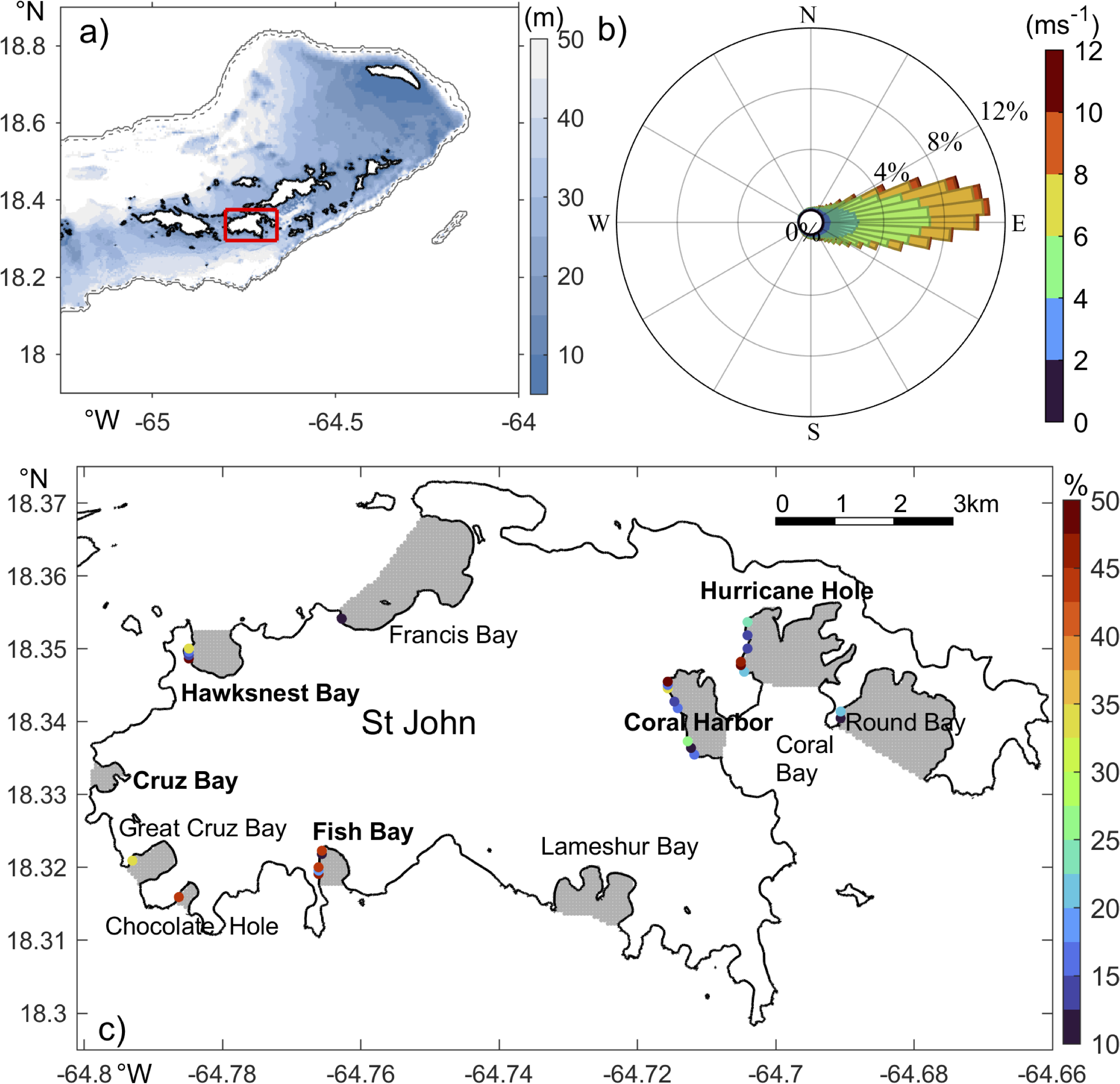
Figure 1. Maps of (A) the model domain and bathymetry and (C) the St John study region, and (B) wind rose of 2016-2022 ERA5 hourly wind, with 5° directional beam. Thick black lines in (A, C) mark coastlines. In (A), gray dashed and solid lines are 100 and 300 m isobath contours, respectively; The red rectangle marks area of (B, C), Gray areas mark regions of particle release in 10 targeted bays; The bays with names in bold are selected for detailed dynamic analysis; Colored dots in the bays indicate spots of surface particle accumulation with the color depicting percentage of surface particle remaining in the bay 10 days after release (note the lower cutoff limit of 10% for display).

Figure 2

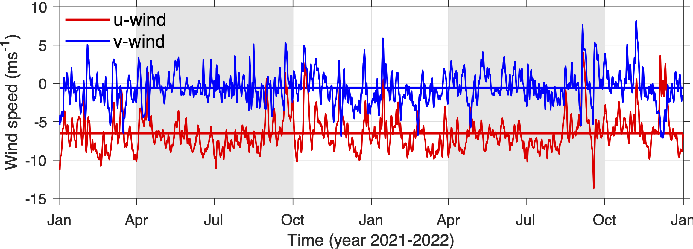
Figure 2. Time series of daily mean eastward (u) and northward (v) winds. Thick lines are the 2-year mean winds. The gray shadings mark summer seasons.

The shoreline of St. John is complex and incised by numerous shallow bays of different shapes and sizes (Figure 1C). The largest one is Coral Bay to the southeast of the island, with a width of ~3 km and depth of<20 meters. It contains several smaller inner bays of ~1 km wide and<10 m deep, including Coral Harbor, Hurricane Hole, and Round Bay. Other bays around the island are mostly 500-1500 m in width. Some prominent ones are Lameshur Bay and Fish Bay on the south shore, Chocolate Hole, Great Cruz Bay, and Cruz Bay on the west shore, and Hawksnest Bay and Francis Bay on the north shore. Because of the different shapes, sizes, and orientations, hydrodynamic conditions in the bays presumably vary. However, the exact hydrodynamic differences across the bays remain unclear. Meanwhile, characteristics of ecosystems in the coastal bays differ. For instance, the Coral Bay region has a high coverage of coral reefs, while the bottom of Fish Bay is mostly covered by seagrasses (Zitello et al., 2009). Induced by changes in local and large-scale processes, the marine habitats in those coastal bays are also undergoing major changes, such as rapid degradation of the coral reefs (e.g., Rogers and Miller, 2006; Edmunds, 2013; Becker et al., 2020; Levitan et al., 2023; Godard et al., 2024). It is thus important to understand the changes in those bays and their connection to the large-scale oceanographic processes.

This study is motivated by the long-term goal to provide a detailed description of the spatiotemporal variability of the physical environment in the coastal bays around St. John for ecological studies and effective resource management. As a first step toward the goal, this work focuses on bay-averaged residence time and investigates its temporal and cross-bay variability in bays of different hydrodynamic conditions. We also investigate the impacts of major forcings on the variation in the residence time of the bays. The realistic high-resolution numerical ocean model described in Part I (Zhang et al., 2025) and a particle tracking model are used here. Section 2 provides details of the model configuration and analysis methods. Modeled particle dispersal in local bays is then described in Section 3, followed by a discussion of impacts of major forcing in Section 4. A summary of the results is provided in Section 5.

2 Methods

The realistic high-resolution St. John hydrodynamic model described in Part I (Zhang et al., 2025) is also used in this study. It is based on the Regional Ocean Modeling System (ROMS; Shchepetkin and McWilliams, 2005; Haidvogel et al., 2008) and covers the shelf around Virgin Islands (Figure 1A) with a horizontally uniform grid resolution of 50 m around St. John and 25 terrain-following vertical layers. To parameterize vertical mixing, the model uses a general length scale turbulence closure k-kl scheme (Warner et al., 2005). Chapman (1985) and Flather (1976) boundary conditions are applied on all 4 open boundaries to simulate the evolution of sea level and 2-dimensional momentum. Fourteen tidal constitutes, including K₁, O₁, P₁, M₂, S₂, N₂, Q₁ are imposed on the open boundaries. To incorporate the large-scale oceanic forcing, bias-corrected velocity, temperature, and salinity fields from the Hybrid Coordinate Ocean Model (HYCOM) global ocean forecasting system (Cummings and Smedstad, 2013), are prescribed on the open boundaries. The temporally evolving 3-dimensional HYCOM temperature and salinity fields are also prescribed in a boundary nudging zone (see Part I for details). The model is forced on the surface by momentum, heat, and salt fluxes computed from the hourly ERA5 meteorological conditions (Hersbach et al., 2020) using bulk parameterization (Fairall et al., 2003). Note that surface waves that can affect particle dispersal through Stoke drift and vertical mixing are not considered in this work and will be included in future studies. As demonstrated in Part I, the model captures observed spatial and temporal variability of tides, temperature, and salinity around St. John. Modeled hydrodynamic fields in 2021-2022 are used in the analysis here.

An offline particle tracking model, ROMSPath (Hunter et al., 2022), is used to simulate the dispersal of particles in the coastal regions around St. John. Built upon the Lagrangian TRANSport (LTRANS) model (North et al., 2008), ROMSPath was designed to complement ROMS output and calculate particle trajectories with high accuracy. In this study, 3-dimensional hourly velocity field from the ROMS-based St. John model is used to drive the ROMSPath calculation of particle trajectories with a time step of 60 s. A total of 725 particle tracking simulations are conducted, with one simulation starting on each of the days between January 5, 2021, and December 31, 2022. In each simulation, particles are released at every model grid within the 10 target bays around St. John (Figure 1C) at the GMT mid-night of each day. Their trajectories are then tracked for 30 days, and particles released in different bays are counted separately. The 30-day simulation window is within the duration range of planktonic larval phase of typical coral species in the region (Miller et al., 2020). Note that the number of particles released in each bay changes with the bay area or volume, depending on the particle type (see below). However, because this study focuses on statistical analyses of particle cluster quantities normalized by particles numbers, the results do not depend on particle numbers.

Two different types of particles, 3-dimensionally distributed (3D) particles and surface-trapped particles (hereafter referred to as surface particles), are used in this study. The 3D particles are neutrally buoyant and released throughout the water column with a 1‐m interval. They move in the water volume following the 3-dimensional currents from the St. John model. These 3D particles represent neutrally buoyant materials, such as dissolved contaminants and pathogens. Due to bay volume differences, the numbers of 3D particles released in the bays in each simulation vary from 158 to 10003. The surface particles are released at the sea surface and remain at the surface at all times. They move with the modeled surface currents only and represent positively buoyant materials, such as floating sea weeds (e.g., sargassum) and early stage of coral larvae (Szmant and Meadows, 2006). The numbers of surface particles released in the bays in each simulation varied from 30 to 727. Random walk is applied in ROMSPath to mimic the impact of unresolved subgrid-scale turbulence on particle dispersal. The magnitude of random walk in the vertical direction is determined by ROMS-simulated vertical viscosity. In the horizontal directions, a constant turbulence viscosity value of 0.01 m²s^-1 is used. The use of the horizontal random walk also prevents some of the surface- particles from being trapped at the coast.

Ten bays representing different environmental and geographic settings (Figure 1) are selected for the analysis. To estimate residence time of materials remaining in the target bays, we compute the flushing time of the bays from simulated particles. Flushing time, as a measure of mean residence time, is a bay-averaged bulk parameter that describes the general exchange characteristics of a waterbody, such as a bay, with the surroundings (Monsen et al., 2002). Following previous studies (Thomann and Mueller, 1987; Monsen et al., 2002), the flushing time of a bay is defined here as the time at which 37% (e^-1, e‐folding) of the particles released in the bay remains inside (gray lines in Figure 3). It is computed for each simulation with particles released at GMT midnight each day.

Figure 3

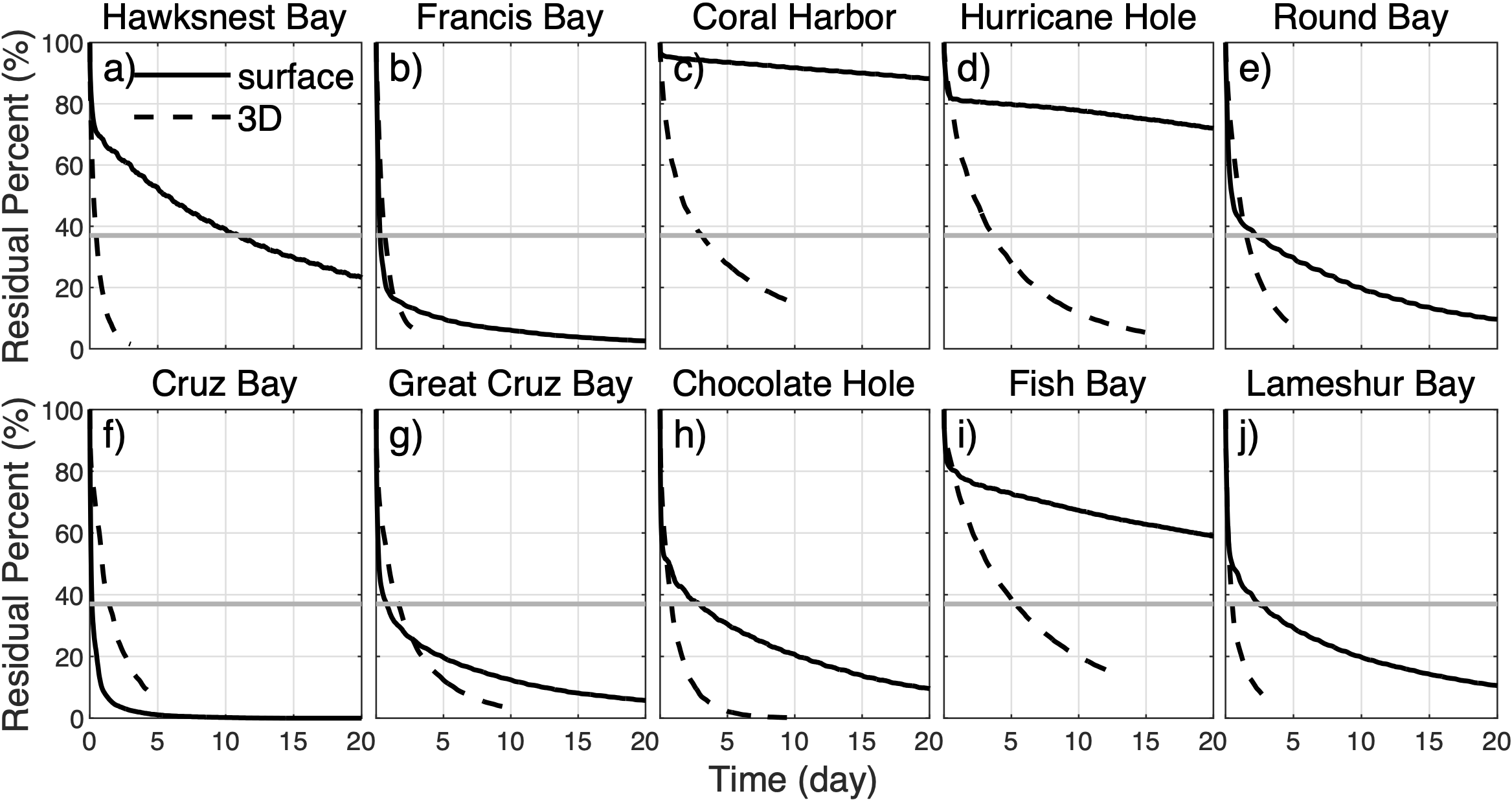
Figure 3. (A–J) Time series of the percentage of surface (black solid line) and 3D (dashed line) particles remaining in the bays after release. The results presented here were computed from all the release simulations in 2021-2022 and represent a two-year mean. The solid gray lines highlight the 37% threshold that the mean flushing times of the bays are defined at (see text).

Material exchange between a bay and the coastal ocean is driven by flows in and out of the bay. However, the calculation of flushing time does not provide any specifics on the exchange flows. To characterize the exchange processes and analyze their dynamics and variability, we compute Lateral Alignment Index (LAI) of the exchange flows (Whitney and Codiga, 2011). LAI is a dimensionless number to quantify the cross-sectional pattern of the exchange flow between a bay and coastal ocean. Following Whitney and Codiga (2011), we first compute the net flux ratio- ($N_f$) of the flow at a site on a cross-bay section,

$\begin{array}{ll}{N}_f=\frac{\left|{\int }_{-h}^{\eta }udz\right|}{{\int }_{-h}^{\eta }\left|u\right|dz}, & (1)\end{array}$

where z is the vertical coordinate, η is sea surface height, h is water depth, and u = u(z) is the velocity normal to the section. $N_f$ equals 1 if the flow at the site consists of pure inflow or outflow over the water column. $N_f$ equals 0 when the inflow completely balances the outflow, resulting in a net flux of 0 at the site. LAI is the cross‐sectional average of $N_f$, that is,

$\begin{array}{ll}LAI=\frac{1}{L}\underset{0}{\overset{L}{\int }}{N}_{f}dx.& (2)\end{array}$

Here, x is the coordinate in the cross-bay direction, and L is the width of the bay at the site. Thus, LAI is also between 0 and 1. A small LAI indicates that the exchange flow has a strong vertical shear with inflows being either over or below outflows. Conversely, LAI being close to 1 signifies a laterally sheared exchange flow with inflows and outflows running side by side.

To understand the mechanism of surface flow driving strong temporal variation in the flushing time of surface particles, Self-organizing Map analysis is used to identify major patterns in the spatial distribution of surface particles in some of the bays. Self-organizing Map is an unsupervised machine learning technique used to produce a low-dimensional representation of a higher-dimensional data set while preserving the topological structure of the data. Essentially, it is a type of neural net clustering analysis (Kohonen, 2001). The method has been successfully used in physical oceanography to identify clusters of flow patterns from temporally-varying spatially-distributed velocities (e.g., Liu and Weisberg, 2005; Meza-Padilla et al., 2019). Here, the number of surface particles in each model grid within a target bay is counted 3 hours after release to generate a daily distribution map of the particles. After that, an empirical 2 $\times$ 2 self-organizing map is applied to the 725 daily distributions of surface particles to give physical meaningful clusters. The training algorithm assigns each of the 725 days to one of the four clusters. To examine the cluster patterns, the modeled distributions of particles 3 hours after release on all days in the same cluster are averaged, resulting in 4 distinct particle distribution patterns in the source bay. Additionally, the modeled hourly surface velocity fields and ERA winds on all days in the same clusters are also averaged to examine the influence of surface flows and winds on the particle distribution.

3 Results

3.1 General pattern of residence time of 3D particles

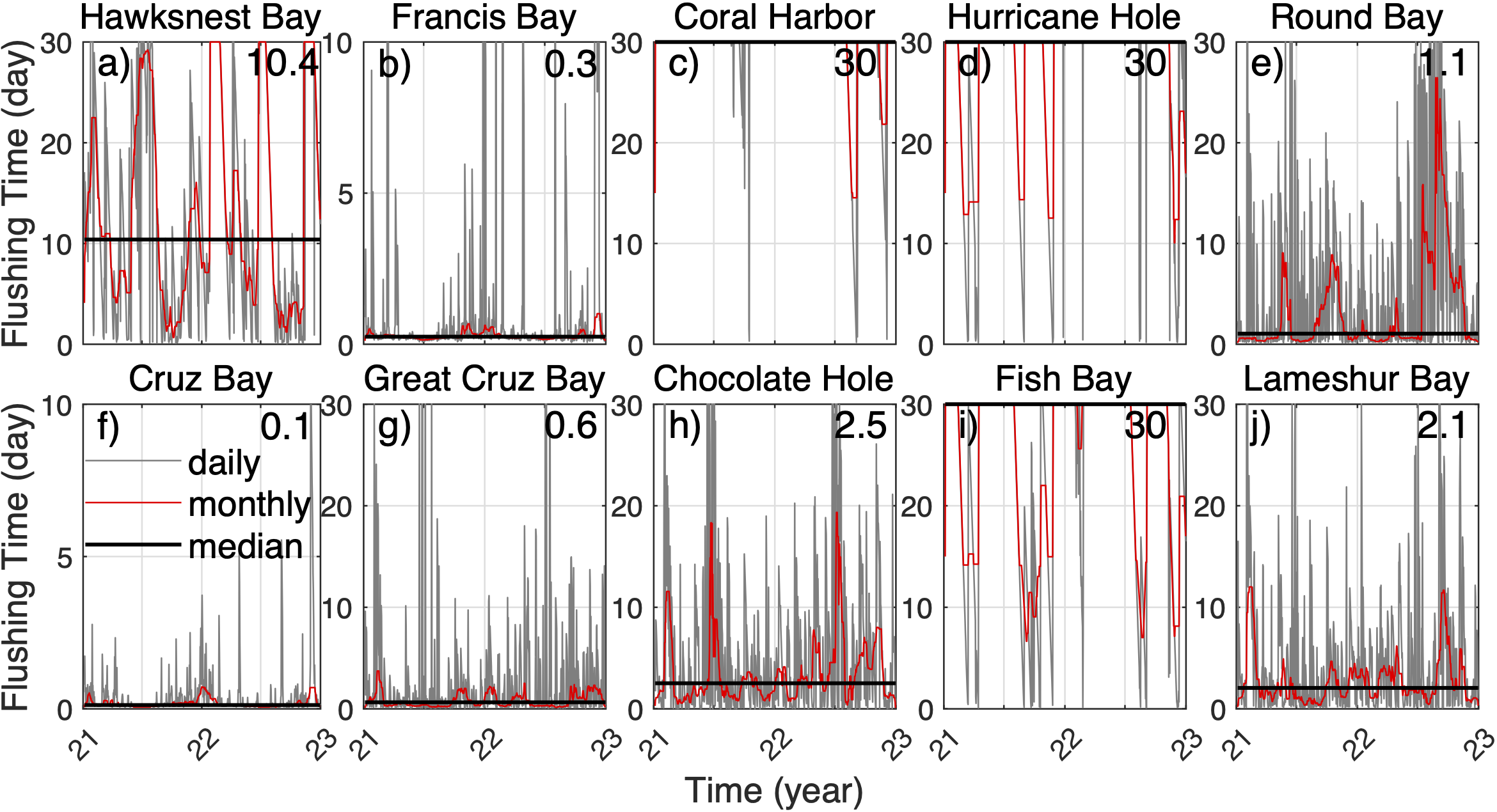
After being released in the St. John coastal bays, neutrally buoyant 3D particles are gradually carried out of the bays by the bay-shelf exchange flow, and the percentages of particles remaining in their source bays gradually decrease (Figure 3). The rates of decrease vary dramatically between different bays. To understand the particle dispersal pattern, we quantify the mean residence time, i.e., flushing time, of 3D particles in the coastal bays of St. John and analyze the mechanisms of variability in flushing time. Flushing times of 3D particles in the bays in 2021‐2022 show significant variability among the bays. The median flushing time is about 1 day in most of the bays (thus relatively high water turnover), 3 days in Coral Harbor, 4 days in Hurricane Hole, and 6 days in Fish Bay (thus relatively low water turnover; Figure 4). These bays vary in size, ranging from 0.15 to 1.82 km². Notably, Francis Bay is 4 times the size of Hawksnest Bay and 12 times the size of Cruz Bay, yet all three bays have a similar flushing time of approximately 1 day. Fish Bay, which is only 1.4 times the size of Cruz Bay, exhibits a mean flushing time about 4 times longer, with a maximum flushing time ~12 days.

Figure 4

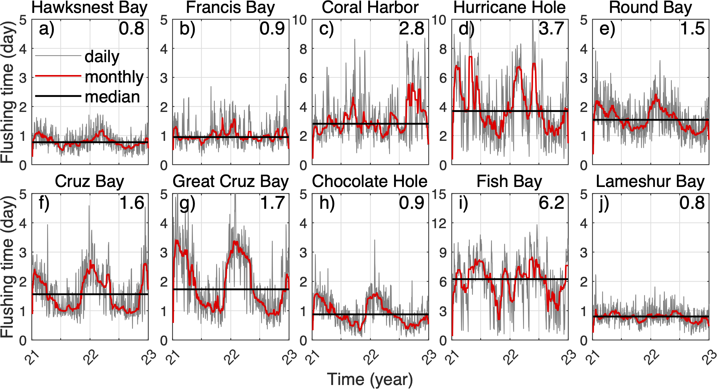
Figure 4. (A–J) Time series of the flushing time of 3D particles at selected bays on each day in 2021-2022 (grey lines), the monthly mean (red lines), and the median value (black lines). The numbers on the upper-right corners of the panels indicate the median values.

The flushing time of 3D particles in most of the bays exhibits distinct seasonal patterns, except for Lameshur Bay (Figure 4). In most of the bays, flushing time is shorter in summer and longer in winter, except in Coral Harbor and Fish Bay. However, the exact timing of these seasonal shifts, the durations of long and short flushing times, and the magnitude of the seasonal variation differ among the bays. For example, flushing times of Hawksnest Bay reach their annual high in February and annual low in July. Cruz Bay, Great Cruz Bay, Chocolate Hole, and Round Bay have the longest flushing time in January and the shortest in November. Hurricane Hole exhibits an annual high‐to‐low ratio of ~10, with two peaks each year. In Fish Bay and Coral Harbor, there are strong variations in flushing time over synoptic time scales. In Coral Harbor, there remains a general tendency of low flushing time in spring and summer and high flushing time in fall. In Fish Bay, despite the large-amplitude high-frequency variation, flushing time is generally high in summer and low in fall and winter (although the median flushing time is comparatively high overall). This can be explained by the key role of winds, besides seasonal variation of the density field, in regulating the bay exchange flows (Section 3.4). Conversely, the variation in flushing time in Lameshur Bay is very small, with no clear seasonal pattern.

3.2 Volume fluxes

Variations in seasonality of flushing time in the bays suggest different processes driving water exchange between the bays and the coastal ocean. To identify the mechanisms, five bays with bold names in Figure 1C and representing different residence time characteristics are selected to investigate the exchange flows, particularly volume fluxes at the bay mouths. For clarity, a 7‐day low-pass filter is applied to all computed volume flux time series. The total outflow fluxes on the bay mouth cross-sections (Figures 5D–F, 6C, D) are computed first. Note that any inflow on the cross-section is neglected in the calculation. The outflow fluxes of Cruz Bay and Hurricane Hole show clear seasonality, but not those of other three bays. In the westward-facing Cruz Bay, the maximum outflow occurs in June-July and the minimum in December-January. This is consistent with the seasonal variation of the zonal wind: persistent easterly winds in summer and large-amplitude fluctuations in winter (Figure 2). That is, persistent easterly winds enhance westward outflow in Cruz Bay, while oscillatory winds result in weak westward outflow there. In Hurricane Hole, situated at the north end of Coral Bay, the maximum outflow occurs in the fall and the minimum in the spring. Examination of the model results shows that the maximum outflow in the fall results from arrivals of the relatively fresh Amazon and Orinoco plume waters from offshore at Coral Bay, which establishes vertical stratification during the fall (Figure 6G) and enhances baroclinic exchange flows between Hurricane Hole and Coral Bay (see Section 3.4).

Figure 5

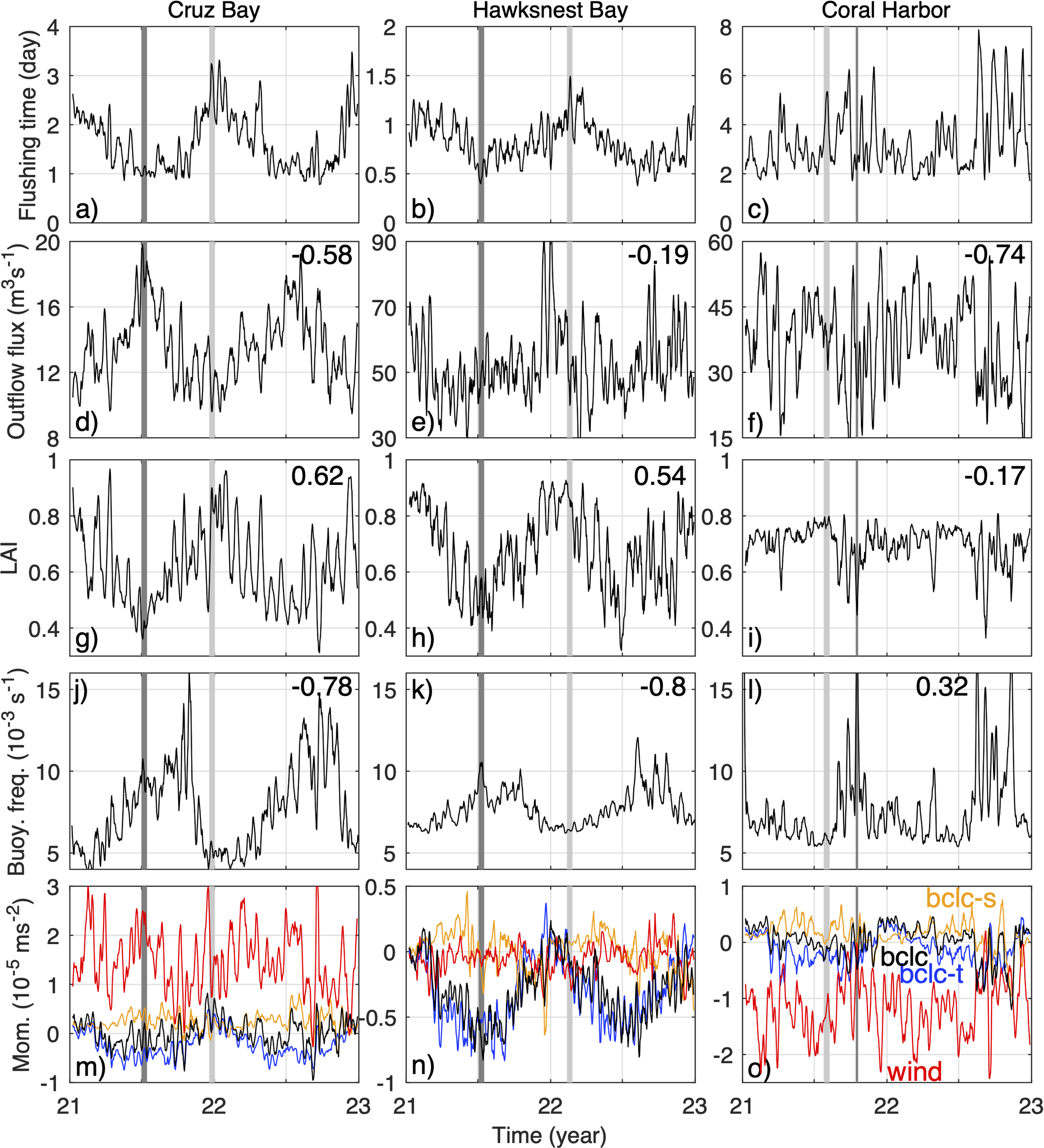
Figure 5. From top to bottom: time series of 7-day averaged flushing time (A–C), outflow flux (D–F), lateral alignment index (LAI) (G–I), Brunt-Väisälä frequency (i.e., buoyancy frequency) (J–L), and along-bay axis momentum terms (Mom.) (M–O) of Cruz Bay (left), Hawksnest Bay (middle), and Coral Harbor (right). The outflow flux, LAI, buoyancy frequency, and moment terms are all averaged on the cross-sections at the bay mouths. For the bottom panel, down-bay is positive; red and black lines denote the along-axis wind stress (wind) and total baroclinic (bclc) terms (two major terms in the flow momentum balance along the bay axes, see text in Section 3.4) in the bays, respectively; the orange and blue lines are the salinity (bclc-s) and temperature (bclc-t) contributions in the baroclinic term. Dark gray and light gray bars in all panels denote selected periods of short and long flushing time, respectively. Numbers at the upper right corners of the panels in the middle three rows depict correlation of the displayed variables with flushing time at the corresponding bay.

Figure 6

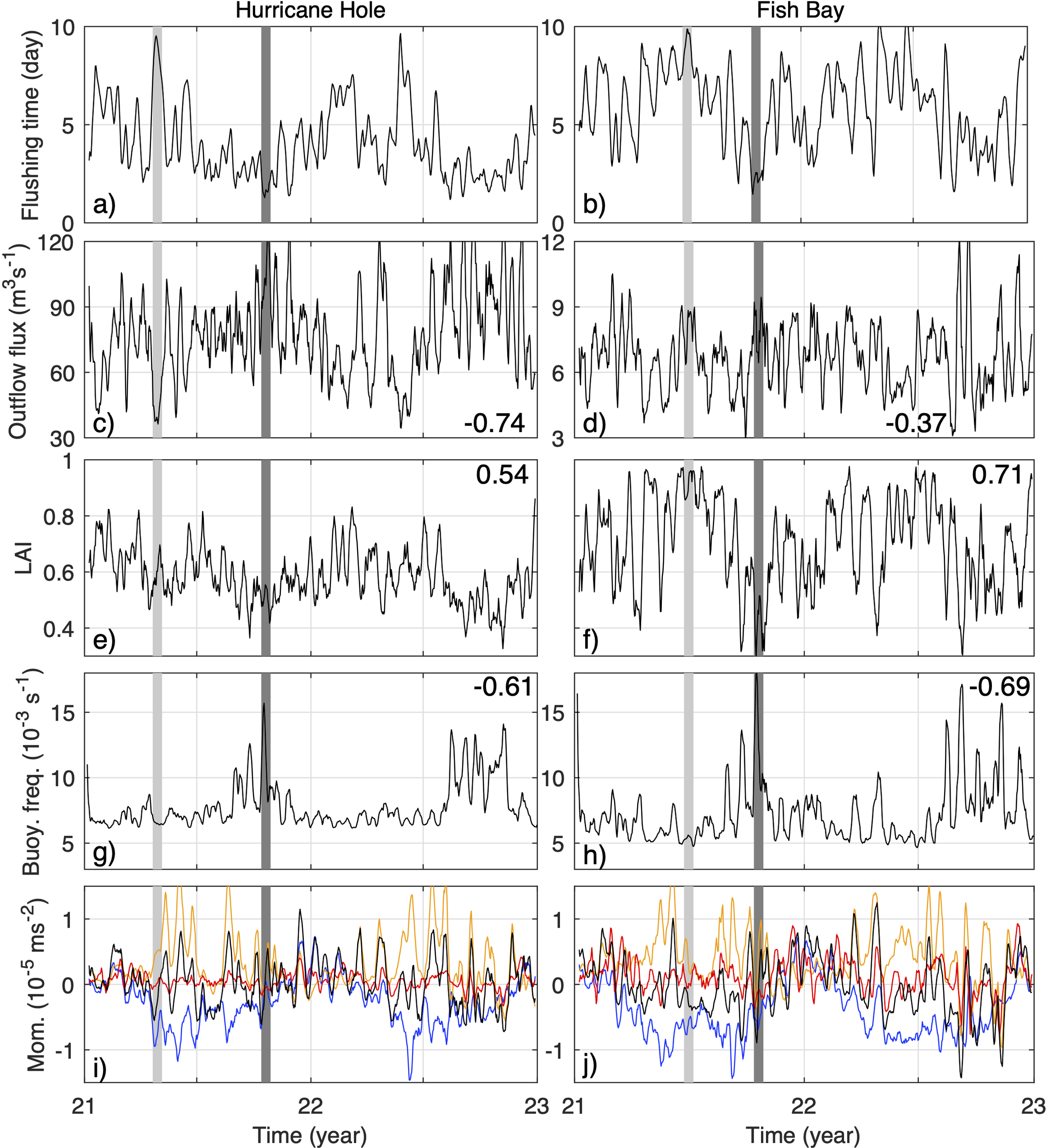
Figure 6. The same as Figure 5 but for Hurricane Hole (A, C, E, G, I) and Fish Bay (B, D, F, H, J).

There are significant negative temporal correlations between the outflow flux on the bay mouth cross-sections and flushing time at Cruz Bay, Coral Harbor, and Hurricane Hole, with respective correlation coefficients of ‐0.58, -0.74, and ‐0.74 and all P-values< 1×10^-10. The negative correlations reflect the expected associations of strong outflow with short flushing times and weak outflow with long flushing times. The lack of strong outflow seasonality at Hawksnest Bay and Fish Bay is likely due to their complex geometry and orientation. Although inverse relationships between outflow flux and flushing time exist in those bays, the correlations are weak, -0.19 and ‐0.37, with respective P-values of 2.6×10^-7 and 1.3×10^-24. Therefore, variations in outflows only contribute weakly to seasonal variations of flushing time in those bays. This is counter-intuitive and will be addressed below.

The lateral alignment index (LAI) of the exchange flows at bay mouths reveals insight into the association of vertical and lateral shear (indicated by small LAI and large LAI, respectively) of the exchange flow with flushing time. Differing from the correlation between outflow and flushing time, the correlation between LAI and flushing time is high in most of the bays, except for Coral Harbor (see Section 3.4 for explanation). For instance, in Hawksnest Bay and Fish Bay, the correlation between LAI and flushing time is 0.5-0.7, much higher than the correlation between outflow and flushing time of 0.2-0.4. In all five bays, LAI exhibits a positive correlation with flushing time, suggesting that vertically sheared exchange flows at the bay mouth shortens the duration of the 3D particles staying in the bay. Conversely, laterally sheared exchange flow tends to keep particles in the bay for longer. To understand this correlation, we selected representative events of short and long flushing time at each bay (dark gray and light gray bars in Figures 5, 6) and examine structure of the exchange flow (Figure 7), particle fluxes (Figure 8), and stratification (Figure 7) during those events. The chosen events are 7 to 15 days in duration, and model quantities are averaged over those periods for analysis.

Figure 7

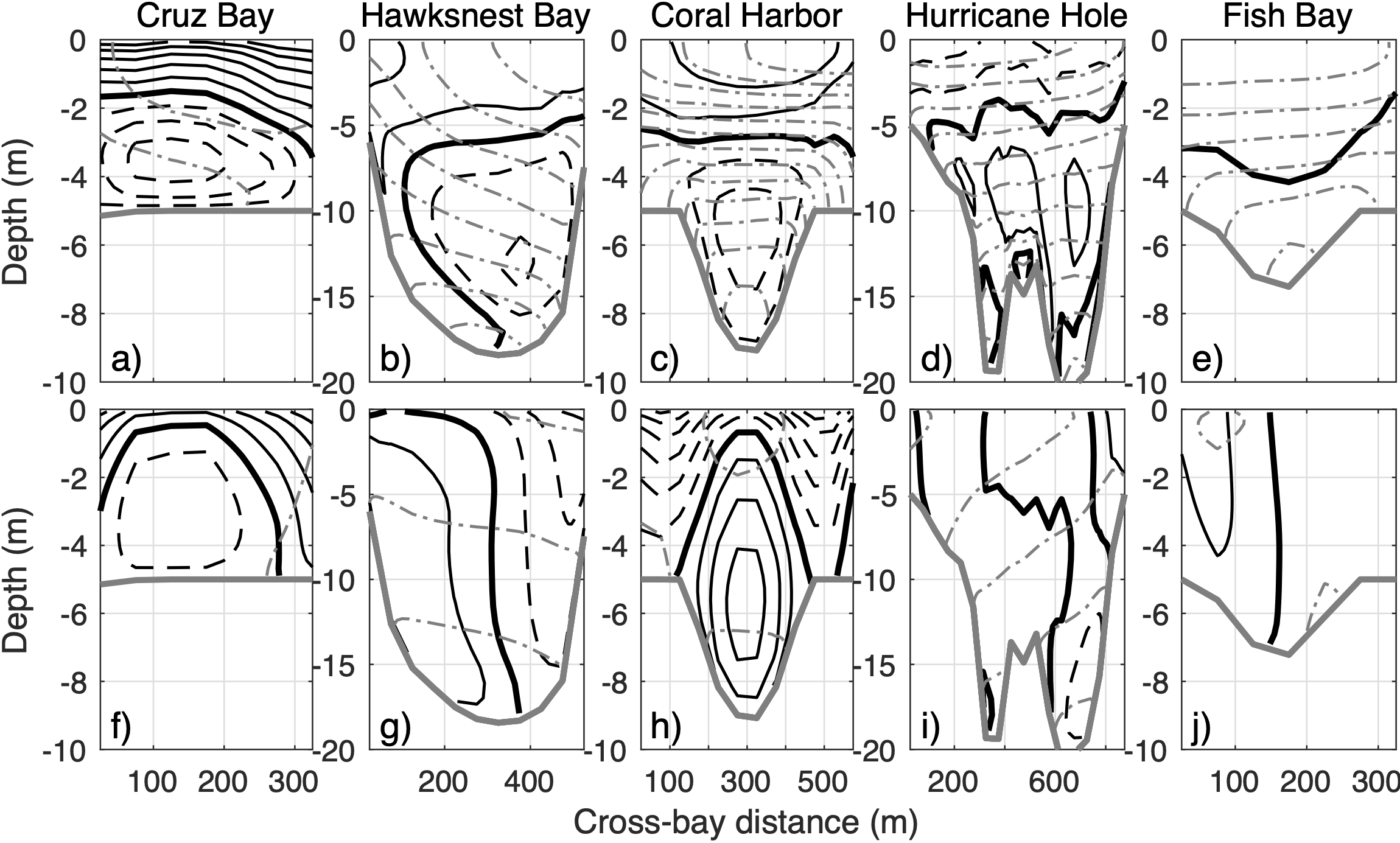
Figure 7. Cross-bay sections of (A–E) outflow (solid black contours with 0.01 m s^-1 interval), (F–J) inflow (dashed black contours), and isopycnals (gray contours with 0.03 kg m^-3 interval) averaged in periods of short (top panels; dark gray bars in Figures 5, 6) and long (bottom panels; light gray bars in Figures 5, 6) flushing time at selected bays. The thick gray line denotes the bottom.

Figure 8

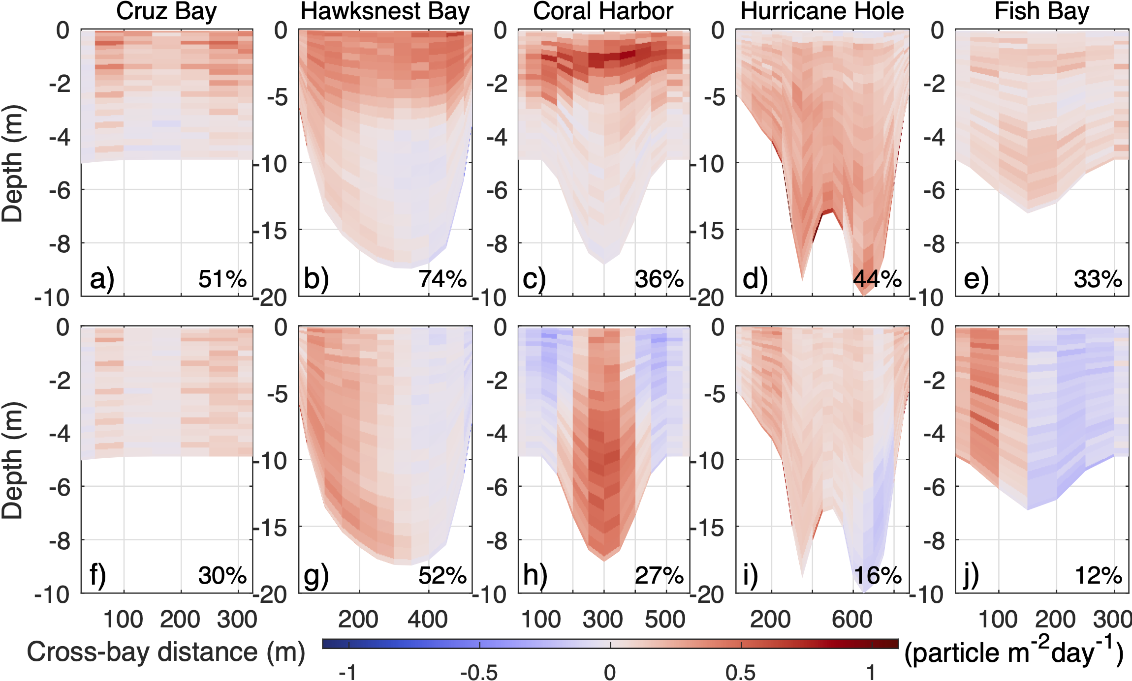
Figure 8. Cross-bay sections of particle outward flux during the first 24 hours after release, averaged over periods (dark gray and light gray bars on Figures 5, 6) of short (A–E) and long (F–J) flushing time. Positive (negative) value means outward (inward) flux. Numbers at lower right corners denote the net percentage of particles across each section leaving the bay averaged over the corresponding periods.

Comparison of the flow cross-sections indicates that, during periods of short flushing time, the exchange flows tend to be vertically sheared with relatively strong vertical stratification on the cross-sections (Figures 7A–E), whereas during periods of long flushing time, the exchange flows are more horizontally sheared with weaker or no stratification in the vertical (Figures 7F–J). In each scenario, cross-sectional distributions of inflows and outflows also differ among the bays. During periods of short flushing time with a stratified water column, vertically sheared exchange flows in most of the bays exhibit a two-layer structure with outflow above and inflow below. However, in the relatively deep Hurricane Hole, the exchange flow is separated into three vertical layers with outflow in the middle and inflow above and below (Figure 7D). Detail analysis indicates that the top-layer inflow in Hurricane Hole results from surface intrusion of the relatively fresh river plume water from offshore. Together with the wind-driven exchange flows below, it forms the 3-layer structure (see Section 3.4 for more explanation). Similarly, during periods of long flushing time, horizontal distribution of the inflow and outflow differ among the bays. In Cruz Bay, the inflow is located in the middle of the channel and outflow on both side flanks (Figure 7F), which is opposite to the exchange flow pattern in Coral Harbor (Figure 7H). In the other three bays, the cross-sections are roughly separated into two lateral sections with inflow and outflow each occupying half.

To quantify the correspondence between stratification and flushing time (Figure 7), we calculated their correlation with the cross-sectionally averaged buoyancy frequency at the bay mouth, which measures mean vertical stratification (Figures 5G–I, 6E, F). Generally, flushing time and stratification have an inverse relationship, meaning that short flushing times occur under high stratification conditions, and vice versa. In particular, the correlation is significant at most of the bays, except for Coral Harbor (numbers in third rows of Figures 5, 6). This is similar to the correction of LAI with flushing time being insignificant only at Coral Harbor. That is, in Coral Harbor, neither vertical shear of the flow nor stratification are significantly correlated with flushing time of 3D particles. The reason for this lack of correlation will be explained later.

3.3 Particle fluxes

To understand the mechanism of stratification and vertical flow shear enhancing particle transport out of most of the bays, we examined the cross-sectional distributions of particle flux at the bay mouths. The fluxes are calculated within the first 24 hours of each particle release simulation and then averaged over the chosen periods of short or long flushing time. In both short and long flushing time scenarios, outward particle flux concentrates in the part of the cross-section having strong outflow (comparing Figures 7, 8). Additionally, the comparison of the panels in each column of Figure 8 shows that the percentage of net particle export on the cross-section (number of outward moving particles minus number of inward moving particles, then divide by the total released particles) at each bay is consistently higher during the short flushing time period than during the long flushing time period.

There are two causes of the differences in net particle export. The first one is directly related to the strength of the outflow, as seen in the case of Cruz Bay. During the short flushing time period, the outflow in the top layer is strong (Figure 7A), resulting in more particles being transported out of the bay (Figure 8A). Conversely, during the long flushing time period, the outflow on the side of the cross-section is relatively weak (Figure 7F), leading to fewer particles being exported there (Figure 8F). This is consistent with the strongly negative correlation between outflow flux and flushing time in Cruz Bay (Figure 5D).

The second cause, as shown in the other four bays, involves the inflow flux (Figures 7B–E, G–J, 8B–E, G–J). Essentially, during long flushing time periods, some of the exported particles are transported back into the bay by the inflow. Notably, in the case of Coral Harbor, the percentage of outward-moving particles on the cross-section is comparable between the long flushing time period (42%) and the short flushing time period (44%). However, during the long flushing time period, 15% of total particles are transported back into Coral Harbor by the inflows on the flanks of the cross-section, nearly double that in the short flushing time condition. Note that 3D particles in Fish Bay can sometimes have flushing time longer than 10 days. During such periods, the ratio of outward to inward moving particle numbers can reach a minimum value of 1.3, significantly lower than the normal range of 2.2 to 5.3 observed in the other cases. This indicates that a significant portion of the particles released in Fish Bay can be carried back into the bay, resulting in long flushing time of 3D particles in the bay at times.

To illustrate this effect of re-entry of 3D particles on flushing time, we use Hawksnest Bay on the north shore as an example and examine the pattern of particles crossing the bay mouth section in the selected periods of short and long flushing times, July 04, 2021, and February 20, 2022, respectively. On July 04, 2021, among the 1262 particles crossing the bay mouth section, 1210 (96%) exit the bay (Figure 9A), and only 52 (4%) re-enter the bay (Figure 9B). In contrast, on February 20, 2022, among the 986 particles crossing the bay mouth section, 769 (78%) exit the bay (Figure 9C), and 19% reenter the bay. Therefore, reentry of the particles greatly increases the overall flushing time of 3D particles in the bay.

Figure 9

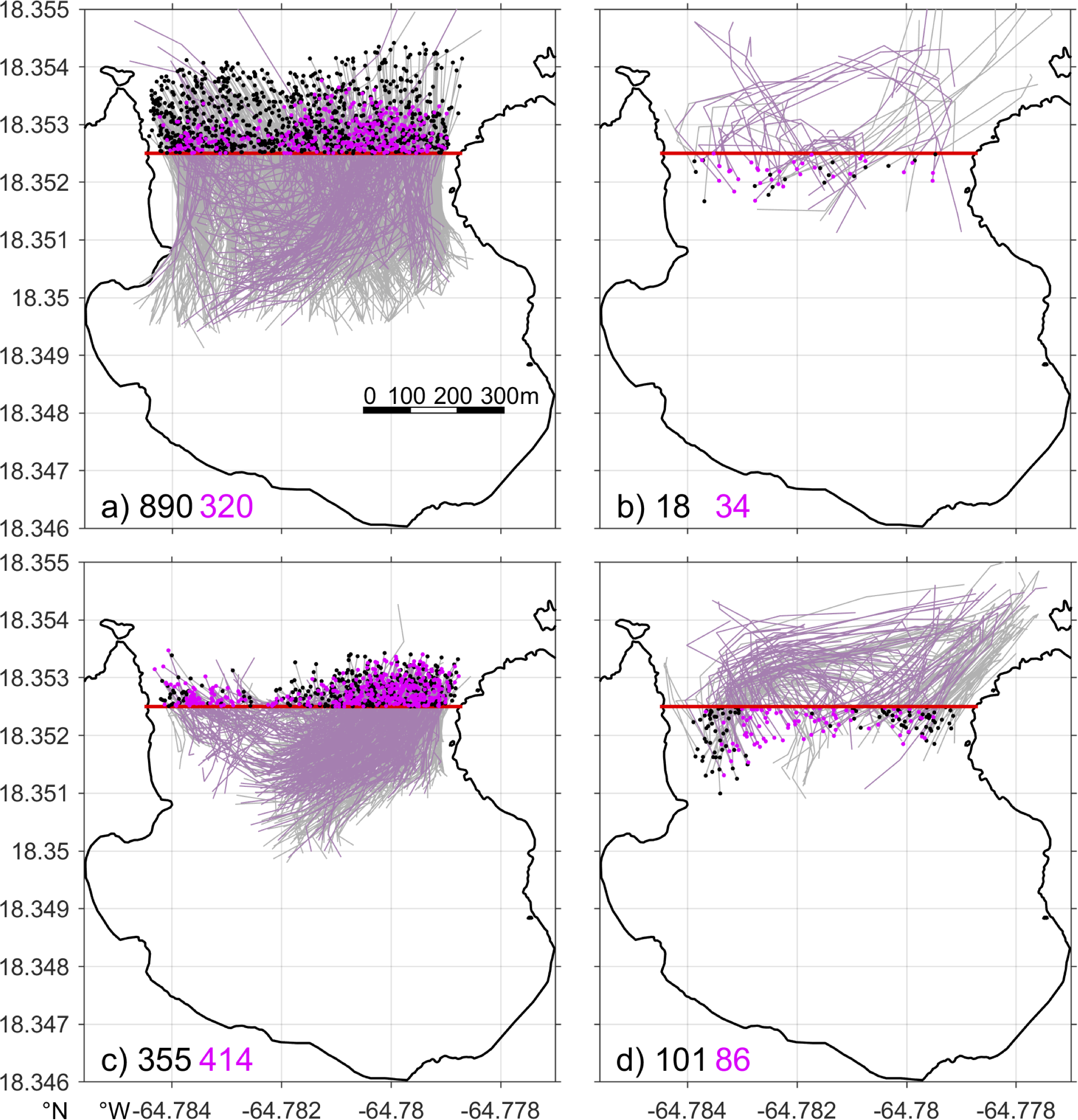
Figure 9. Trajectories of 3D particles in 2-hour windows around the times of the particles crossing the mouth of Hawksnest Bay either leaving (A, C) or re-entering (B, D) the bay on July 04, 2021 (top; dark gray in Figure 5B) and February 20, 2022 (bottom; light gray in Figure 5B). Red thick lines denote the bay mouth section; gray and light magenta lines denote trajectories of the particles that cross the bay mouth section at a vertical position above and below the 5 m depth, respectively; black and magenta dots denote the positions of the corresponding particles after crossing the section; numbers at lower left corners denote the corresponding particle numbers depicted in the panels.

3.4 Momentum analysis

To understand the driver of the temporal variabilities of volume fluxes, particle fluxes, and flushing time described above, we examine the roles of wind stress and baroclinic pressure gradient force, two major forces in the flow momentum balance along the bay axes. These forces are averaged on the cross-sections at the bay mouths. The baroclinic pressure gradient force is decomposed into contributions of salinity and temperature variation. According to the relative strengths of the forces (bottom panels in Figures 5, 6), dynamics of the bay exchange flow can be separated into two types: wind‐dominant or baroclinic‐dominant, with the orientations of the bays being a major determining factor.

Wind-dominant bays include Cruz Bay and Coral Harbor, both of which have axes lying mostly parallel to the dominant easterly wind direction. Comparisons of the flow moment terms show that the primary driving force of flows in those bays is wind stress (Figures 5M, O). For instance, in Cruz Bay, the along-axis wind stress is more than 4 times greater than the total baroclinic pressure gradient term. However, the along-axis wind stress shows only weak seasonal variation, inconsistent with the seasonally varying flushing time (Figure 5A). Their correlation is only 0.07 and insignificant. Meanwhile, the relatively weak baroclinic term shows a clear seasonality, primarily driven by seasonal changes in temperature.

Detailed analysis indicates that this apparent inconsistency results from the interaction between winds and temperature induced stratification in the bay. Winds in the summer, despite being slightly stronger, cannot fully break the water column stratification, which allows temperature-induced stratification to establish a vertically sheared exchange flow. Easterly winds in the summer are thus able to drive westward surface outflow in Cruz Bay (Figure 7A), which facilitates rapid particle export from the bay and lowers the flushing time. In contrast, during winter, stratification breaks down and the wind-driven exchange flow becomes laterally sheared (Figure 7F). It allows some particles to be carried back into the bay and increases the flushing time, as stated in Section 3.3. Therefore, even though winds primarily drive the circulation in Cruz Bay, temperature-induced stratification determines the structure of the exchange flow and then temporal variation of the flushing time.

In Coral Harbor, dominant easterly winds are aligned with the up‐bay direction, creating inflow on the surface and the shallow flanks, as well as a subsurface outflow in the deep channel (Figure 7H). While the subsurface outflow carries particles out of the bay, the inflow on the flanks brings many of the exported particles back into the bay, resulting in a relatively long flushing time (Figure 7H). The wind-driven surface inflow also induces a sea level set up in the bay and an eastward barotropic pressure gradient force pointing out of the bay, primarily balanced by the westward surface wind stress (not shown). When the easterly wind weakens or reverses direction, the barotropic pressure gradient force associated with the sea level setup in the bay drives an eastward outflow on the surface. Meanwhile, the along-axis baroclinic pressure gradient associated with the temperature difference inside (warmer) and outside (colder) of the bay drives a subsurface inflow (Figure 7C). This pattern resembles the estuarine exchange flow (MacCready and Geyer, 2010). The associated surface outflow tends to carry a large number of particles out of the bay (Figure 8C), resulting in a shorter flushing time. These wind-fluctuation-induced changes in exchange flow differ from the relatively persistent stratification-induced exchange flow and are not completely vertically or horizontally sheared. Consequently, flushing time of 3D particles in Coral Harbor is only weakly correlated with LAI and stratification (Figures 5I, L).

In Hawksnest Bay, Hurricane Hole, and Fish Bay, which are oriented mostly in the north-south direction perpendicular to the dominant easterly wind direction, the main force driving flow is the baroclinic pressure gradient force along the bay axis. For instance, in Hawksnest Bay, the exchange flow is primarily driven by temperature‐induced baroclinicity (Figure 5N). During summer, such as, on July 04, 2021, water in the shallow bay warms up more rapidly than water on the deeper shelf. As a result, the relatively cold and dense shelf water intrudes into the bay at the bottom, while the warmer bay water exits from the surface (Figure 7B). The surface outflow drives most of the particle export (Figure 8B). On July 04, 2021, 890 (75%) of the 1210 particles leaving the bay cross the bay mouth in the surface 5 m (grey lines in Figure 9A). After leaving the bay, most of the particles remain in the surface layer on the shelf because the shelf water column is also stratified during the period. Since the intruding shelf water is concentrated in the bottom layer, most of the exported particles cannot re-enter the bay. Consistently, among the 52 particles that re-enter the bay on that day, 34 (65%) cross the bay mouth section in the bottom layer. Thus, the vertically sheared exchange flow results in a relatively short flushing time.

In winter, when the temperature difference between the bay and shelf waters reduces, vertical stratification mostly disappears, and the density‐driven exchange flow is weakened. It causes the bay-shelf exchange flow and the particle outflux to be laterally partitioned (Figures 7G, 8G). Correspondingly, the numbers of particles leaving the bay in the surface and bottom layers are similar (Figure 9C), so are the particles re-entering the bay (Figure 9D). Therefore, weak vertical stratification and flow shear in the bays and shelf allow more particles to re-enter the bays and lead to long flushing times of 3D particles in the bays.

In the south-facing Hurricane Hole and Fish Bay, the exchange flow is influenced by both local temperature changes and the influx of fresher water from the south. During late spring and early summer, before the vertical thermal stratification develops in the bays, the arrival of low-salinity water from the Amazon River plume generates an along-axis baroclinic pressure gradient force in the bays, opposing the along‐axis baroclinic force induced by the temperature difference between the bay and shelf waters (Figures 6I, J). The competition of the along-axis temperature and salinity gradients causes strong temporal fluctuations of vertically-sheared exchange flows and, at times, complications in the vertical structure of the exchange flow, such as the three-layer structure at Hurricane Hole (Figure 7D). These factors together drive strong fluctuation in the flushing time of 3D particles (Figures 6A, B). In summer and fall, when vertical thermal stratification is well‐established in the bay, the arrival of the low-salinity water from the Orinoco River plume is unable to overcome the thermal stratification and significantly alter the vertically sheared exchange flow. This results in a relatively persistent, vertically sheared exchange flow and then relatively low flushing time (Figures 6A, B). That is, few particles can re-enter the bays after they are advected out. In winter, when the bay and shelf waters have similar temperature and salinity with weak lateral density difference, the exchange flow slows down, which reduces the rate of particles being advected out of the bays and leads to a generally high flushing time.

To summary, a general pattern observed here is the strong connection of vertical shear in the bay-shelf exchange flow and vertical stratification with the flushing time of 3D particles: stronger stratification and vertical shear of the exchange flow, as indicated by smaller LAI, are associated with a short flushing time of 3D particles in the bays, while weaker stratification and vertical shear are associated with a long flushing time. This connection is driven by the vertical stratification and lateral mixing in the open coastal region outside of the bays. Essentially, during unstratified seasons, the influx and outflux of particles are laterally separated at the bay mouths (e.g., Figures 7F, G, I, J). The 3D particles are distributed throughout the water column. Once the particles leave a bay, they are mixed on the open shelf, and a substantial amount of the particles are entrained into the inflows and return to the bay. This results in a long flushing time of 3D particles in the bay. However, during stratified seasons with either temperature- or salinity-driven stratification, waters in the bay and on the open shelf are all stratified. The exchange flows at the bay mouths are vertically sheard with low LAI. That is, the outflow is concentrated in the surface layer, and the inflow is mostly in the deeper layer. The 3D particles are carried out of the bays in the surface layer. After leaving the bay, most of them remain in the surface layer of the stratified shelf. Since the water flowing into the bay from the shelf is from the subsurface, few particles can return to the bay. This results in a short flushing time of 3D particles in the bay.

3.5 Surface-trapped particles

Simulations of surface particles show that their rates of leaving the source bays differ from those of the 3D particles. The leaving rates of surface particles are slower in some of the bays, such as Hawksnest Bay, Coral Harbor, Hurricane Hole, Chocolate Hole, Fish Bay and Lameshur Bay, but faster in the other bays (Figure 3). These differences are also reflected in the flushing times of surface particles (Figure 10), which are different from those of 3D particles (Figure 4). Flushing times of surface particles also show temporal variation over a wide range (Figure 10). In particular, bays with a wide westward opening, such as Cruz Bay and Francis Bay, typically have median flushing time of surface particles less than 0.5 days, albeit with occasional occurrences of much longer flushing times. In contrast, bays with a southward or eastward opening have significantly longer median flushing time. Notably, Fish Bay, Coral Harbor, and Hurricane Hole have flushing time exceeding the simulation period of 30 days (Figures 10C, D, I).

Figure 10

Figure 10. (A–J) Time series of the flushing time of surface particles at selected bays on each day in 2021-2022 (grey lines), the monthly mean (red lines), and the median value (black lines). The numbers on the upper-right corners indicate the median values. Note that in some of the bays, the flushing time is sometimes longer than the 30-day simulation period.

A detailed analysis shows that surface trapping of the particles is the primary factor responsible for the vast difference in flushing times in the bays. In the bays with a wide westward opening, surface particles are quickly carried out of the bays by the dominant westward surface flows driven by the prevailing easterly winds. Consistent with the seasonal variation in the easterly wind strength (Figure 2), flushing times in those bays, such as Francis Bay and Cruz Bay, show clear seasonality with short flushing time in summer and long flushing time in winter (e.g., Figures 10B, F).

In Round Bay, which has a southwestward opening, the median flushing time of surface particles is relatively low, but the flushing time changes dramatically over time (Figure 10E). To understand the dynamics, we examine the clusters of surface particle distributions in Round Bay obtained from the self-organizing map analysis and correlate them with winds and surface flows over the same days (Figure 11). The first two clusters show bands of concentrated particles in the bay mouth aligned with strong outflow (Figures 11A, B). Winds during those days are generally southwestward, approximately aligned with the bay axis. This indicates that the southwestward wind drives a strong surface outflow, which carries much of the surface particles out of the bay. Correspondingly, the flushing times during those days are short, with median values of 0.3-0.4 days (Figures 11A, B). This pattern is similar to the process causing low flushing time in the aforementioned westward-facing bays.

Figure 11

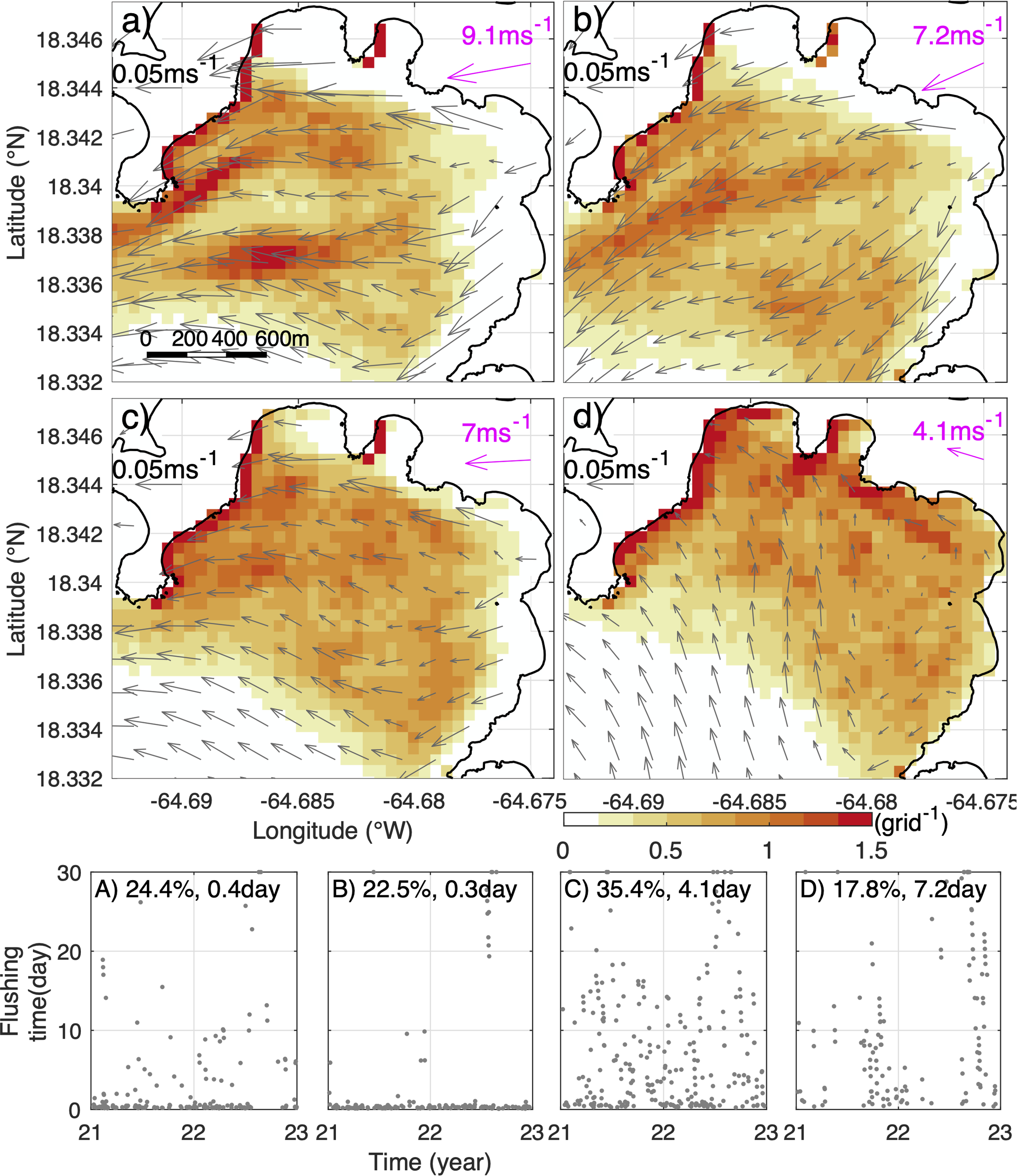
Figure 11. (a-d) Mean distribution of the surface particles (colored) 3 hours after release in Round Bay given by a 2×2 Self-Organizing Map applied on results of daily particle tracking simulations in 2021-2022. Gray arrows denote mean surface currents during the corresponding times with the scales provided at the upper-left corners. Magenta arrows and numbers depict the corresponding mean wind speed and direction. (A–D) flushing times of the surface particles released on the days under different patterns characterized by the Self-Organizing Map analysis. Numbers at the top of (A–D) are the percentage of times captured by each pattern and the median flushing time of the releases on the days in each pattern.

The other two clusters in Round Bay show a high concentration of surface particles on the northwest coast of the bay (Figures 11C, D). In Cluster 3, both winds and surface flows are mostly westward, while they are mostly northwestward in Cluster 4. This suggests that, during those periods, surface particles released in Round Bay are pushed to the western ends of the bay and trapped there (colored dots in Figure 1C) by the persistently westward or northwestward surface flows driven by the easterly or southeasterly winds. Because the particles are surface-trapped, they cannot move downward into deeper part of the bay with the water and are thus stuck to the coast, accumulating there. This differs from the 3D particles that can move into the deeper part of the water column and then be transported out of the bays. As a consequence of the wind-induced trapping on the west coast of the bay, flushing times of surface particles in Round Bay in Clusters 3 and 4 are long with median values of 4 and 7.2 days, respectively (Figures 11C, D).

A similar pattern of surface particle distributions exists in Great Cruz Bay and Chocolate Hole. Interestingly, flushing times of surface particles in Great Cruz Bay and Chocolate Hole show seasonality, with longer flushing in summer and shorter in winter (Figures 10G, H). This results from the persistent easterly winds in summer pushing a small amount of the surface particles to the western end of the bays and keeping them there (colored dots in Figure 1C). In winter, the fluctuating winds allow the particles being pushed to the western end to be unstuck and then transported out of the bay.

In Hawksnest Bay, Coral Harbor, Hurricane Hole, and Fish Bay, with a northward, eastward, southward, and southward opening, respectively, a substantial amount of the released surface particles remains in the bays for a long time. Consequently, flushing times of the particles are persistently high in these bays (Figures 10A, C, D, I). Examination of the model results confirms that surface particles released in those bays are trapped at the western ends of the bays (colored dots in Figure 1C) by the persistent westward surface flows driven by the prevailing easterly winds.

Therefore, easterly winds have competing impacts on the flushing time of surface particles in the bays around St. John. Easterly winds can drive surface particles out of a bay quickly, resulting in a short flushing time if the bay has a westward opening. Conversely, they can trap particles at the western end of a bay and cause long flushing time of the particles in the bay if the opening of the bay is not completely westward.

4 Discussion

This study demonstrates significant temporal and cross-bay variability in the exchange processes between coastal bays around St. John and the open shelf, driven by temporal variation in stratification, winds, and bay orientation. Changes in the exchange processes result in strong variations in the flushing time of both 3D and surface particles in the bays. As demonstrated in Section 3, intrusion of the Amazon and Orinoco River plumes can modify the near-shelf density structure and affect particle transport. Other factors, such as tides and waves, could also affect the dispersal of the particles. The wave impact will be considered in future studies. Here, we provide quantitative measures of the potential impact of tides and the river plumes.

4.1 Tides

As demonstrated in Part I, tides have a strong impact on the flows in the open coastal regions around St. John. However, tides do not appear to be a major driver of the water exchange between the bays and the shelf. One way to estimate the influence of tides on the flushing time of water in a bay is to apply the tidal prism method, using information on bay geometry and tidal ranges (Dyer, 1973). The flushing time driven by tidal flows can be estimated as

$\begin{array}{ll}{T}_t=\frac{VT}{(1-b)P}& (3)\end{array}$

where, V is the bay volume, T is the tidal period, P is the tidal prism, defined as the volume between high and low tidal elevations, and b is an empirical factor between 0 and 1, describing the fraction of exported water returning to the bay at each tidal cycle. Assuming the bay has a uniform depth h and no returning water (i.e., b = 0, which gives the shortest flushing time), the flushing time driven by the tides with tidal range of R is

$\begin{array}{ll}{T}_f=\frac{h}{R}T& (4)\end{array}$

The mean depth of most St. John bays is h = 5 m, and the tidal range during a spring tide period is R = 0.4 m. These give $T_f$ = 13 days, which is much longer than mean flushing times of 3D particles in all bays (Figure 4) and those of surface particles in most of the bays (Figure 10). This suggests that tides are not a major driver of water exchange process between the bays and the open coastal region around St. John. Even in the bays with surface particle flushing time longer than the tidally-driven flushing time, the prolonged particle flushing time is caused by wind-driven trapping of the surface particles on the west coast of the bays. Consequently, tidal flows are unable to move the trapped particles.

4.2 River plumes

Intrusion of the Amazon and Orinoco River plumes from the south during summer and fall can influence the exchange flows of the bays on the south shore of St. John, creating spatial inhomogeneity in the coastal environmental condition. Our model simulations show that plume-induced density gradient can greatly affect the exchange flow of the bays on the south shore. We aim to quantify the influence of the intruding plume on the exchange flow dynamics in these bays by comparing the plume-induced baroclinic pressure gradient force with wind stress, another major force in the along-axis momentum balance.

The model shows that in Hurricane Hole and Fish Bay, wind stresses, ${\tau }_x$, in the along-axis direction of the bays, x, are mostly less than 5×10^-6 m s^-2. For simplicity, we use a linear equation of state, $\text{Δ}\rho =\alpha \text{Δ}T+\beta \text{Δ}S$, to estimate potential temperature and salinity contributions to the baroclinic pressure gradient force. Here, the thermal expansion coefficient α $\approx$ -0.338 kg m^-3°C^-1, haline contraction coefficient β $\approx$ 0.75 kg m^-3 at the temperature and salinity ranges of interests, ΔT is the temperature variation, and ΔS is salinity variation. The vertical integrated baroclinic pressure gradient force in the along-axis momentum balance is

$\begin{array}{ll}P{G}_{bc}=-\frac{g}{{\rho }_{0}h}\underset{-h}{\overset{0}{\int }}(\frac{\partial }{\partial x}\underset{z}{\overset{0}{\int }}\rho dz)dz& (5)\end{array}$

where g is the gravitational acceleration, ρ₀ = 1000 kg m^-3 is the reference water density, and $h\approx 5 m$ is the mean water depth. Assuming the force exerted by a wind stress of -5×10^-6 m s^-2 having the same magnitude as the baroclinic pressure gradient force generated by the along-axis density gradient, and apply the force to the left hand of (3) gives $\partial \rho /\partial x$ $\approx$ 2×10^-4 kg m^-4. Here, we assume a constant along-axis density gradient, $\partial \rho /\partial x$, in the along-axis and vertical directions. The required $\partial \rho /\partial x$ is equivalent to $\partial T/\partial x$ $\approx$ 6×10^-4 °C m^-1 when there is no horizonal salinity gradient (i.e., $\partial S/\partial x=0$), or to $\partial S/\partial x$ $\approx$ 2.7×10^-4 psu m^-1 when there is no horizonal temperature gradient (i.e., $\partial T/\partial x=0$). The St. John bays have a length scale of 500m. Therefore, to balance the wind stress would require a temperature difference between the bay and open coast of 0.3°C when salinity is uniform, or a salinity difference of 0.14 psu when temperature is uniform. The required salinity difference is less than a typical salinity variation of 0.5-1 psu induced by the intrusion of the river plumes. This is consistent with the modeled salinity-driven baroclinic term being dominant in Hurricane Hole and Fish Bay in the summer and fall when the plumes arrive (Figures 6I, J). Therefore, intrusion of the Amazon and Orinoco River plumes from the south can strongly impact the exchange flow and thus water flushing time in the bays on the south shore whose axes are not aligned with the wind direction.

Note that, in bays oriented mostly along the wind direction, such as Cruz Bay and Coral Harbor (e.g., Figures 5M, O) mean wind stresses are at least three times the density-induced baroclinic force. Circulation in those bays is thus mostly wind-driven and substantially less influenced by intruding river plumes.

4.3 Ecosystem implications

The residence time variabilities and the associated drivers demonstrated here have direct implications for differential reef ecosystem dynamics around St. John. The model output is relevant to local biological research, ecological conservation and resource management. Further, this study provides an important framework for other island and coastal communities interested in using hydrodynamic information to guide restoration, conservation and other management activities. Below, we discuss several examples and hypotheses of ecosystem implications.

The timing of the influence of Amazon and Orinoco River plume waters is particularly striking because this summer-fall period of greater intrusions coincides with the general period of spawning and consequent larval dispersal for many fishes and coral in the area (Goodbody-Gringley, 2010; Suca et al., 2020). It is thus possible that greater river plume influx could help move fish and coral larvae out of some of the bays that are directly influenced by the plume waters (e.g., Fish Bay, Lameshur Bay, etc.). For those coral species with relatively short competency periods and able to settle in hours, the intruding plume waters may have a lesser overall effect. For instance, larvae from colonies of the rapidly competent brooding coral, Porites asteroides in Lameshur Bay (Fadlallah, 1983; Edmunds, 2010) might be able to settle quickly before being flushed out by the exchange flows. However, for other spawning coral species with longer development times, there may be more genetic dispersal and overall lower abundances due to larvae being quickly washed out from the bays.

Variation in flushing times in coastal bays likely affect contaminant and disease spread. Stony coral tissue loss disease (SCTLD), a waterborne disease (Walton et al., 2018), has recently impacted the reefs of St. John, resulting in significant coral mortality around the island (Brandt et al., 2021). Disease spreading rates and impact on resident corals varied, which are likely related to the local hydrodynamics. Indeed, some bays, such as parts of Coral Bay, saw a delayed spread of SCTLD, suggesting that the currents noted here were slow to bring the disease to those populations (Brandt et al., 2021). Future studies focusing on finer-scale pathogen/contaminant trajectories and residence times variation using hydrodynamic models covering a larger region will be useful for resource managers to better prioritize mitigation or treatment efforts to certain bays or coastal areas.

This type of high-resolution particle dispersal model can also support restoration activities. For example, it may be most informative to plant corals or consider rebuilding reefs where larvae tend to aggregate or have time to settle, particularly with the development of larval attraction such as sound (Aoki et al., 2024). This could help maintain high reef populations (see particle aggregations in Figure 11). Conversely, management agencies may choose not to put initial resources in areas where larvae may likely to be flushed away. Overall, this information on the physical environment can be vital as managers and stakeholders allocate valuable, limited resources.

One next step of the study is to quantify larval connectivity among key habitats around St. John and the neighboring islands as well as the temporal variability of the connectivity using a high-resolution model covering a larger area. As larval movements in near-shore regions are controlled by fine-scale flow patterns, having a high-resolution hydrodynamic model is key in accurately resolving the transport of larvae from one near-shore region to another (Saint-Amand et al., 2023). Meanwhile, having a sufficiently large model domain covering direct and indirect larval transport pathways is necessary for answering ecological questions related to connectivity among sites far away from each other. The result of this type of model will help reef conservation effort by providing information on which part of the habitat is more effective at seeding the neighboring regions and thus more important for targeted protection (e.g., Storlazzi et al., 2017).

5 Conclusions

Building upon the high-resolution hydrodynamic simulation of the physical environmental conditions around St. John, USVI in Part I, this Part II of the study uses a particle tracking model to simulate dispersal of particles released in coastal bays around St. John without considering the influence of surface waves. Two types of particles are considered in this study, i) three-dimensionally distributed (3D) particles, and ii) surface-trapped (surface) particles. The former could represent neutrally buoyant materials, including dissolved chemical constituents and pathogen, while the latter could represent buoyant materials, such as early-stage coral larvae and Sargassum. Motivated by the long-term goal of providing high-resolution hydrodynamic variability for coral conservation and coastal resource management, this work aims to characterize variabilities of the bay-averaged residence time (i.e., flushing time) of the particles in the bays. Analysis of the model results shows pronounced influences of winds, intruding river plumes, and bay orientation on the residence time of both types of particles.

Mean flushing times of 3D particles in the bays vary from 1 to 6 days, with most of the bays having flushing time of 1-2 days. Flushing time in Coral Harbor and Hurricane Hole in the Coral Bay is 3-4 days, as water in them exhibits a slower exchange rate with the open shelf. Fish Bay on the south shore has the longest mean flushing time of 6 days.

The flushing time of 3D particles in most of the bays display clear seasonality, with a strong correlation with the exchange flow pattern at bay mouths. Short flushing time generally coincides with vertically sheared exchange flow and strong stratification, while long flushing time accompanies laterally sheared exchange flow and weak stratification. The long flushing time results from re-entry of the particles into the bays. During the stratified season, stratification in the open coastal region reduces the chances of exported particles returning to the bay, thereby decreasing the flushing time of the particles within the bays. Momentum analysis shows that exchange flow of a bay with the open coastal region is mostly wind-driven when the bay, such as Cruz Bay and Coral Harbor, aligns with the predominant easterly winds. In bays on the north shore with axes normal to the wind direction, the exchange flows are mostly driven by temperature-induced density differences in and out of the bays. Conversely, in bays on the south shore with axis normal to the wind direction, the exchange flows during the stratified season are mostly driven by surface intrusion of the low-salinity Amazon and Orinoco River plumes from the south.

Simulations of surface particles demonstrate significant variations in their flushing times within bays around St. John, primarily influenced by the opposing effects of the prevailing easterly winds. In bays like Francis Bay and Cruz Bay that face westward, wind-driven westward surface flows quickly carry surface-trapped particles out of the bays through their westward-facing openings, thereby reducing the flushing time. Conversely, in most other bays where the bay axes do not align with the wind direction, the persistent westward surface flows induced by easterly winds cause the surface-trapped particles to accumulate along the western shorelines of the bays, leading to a dramatic increase in flushing time.

The inter-bay and temporal variability of material flushing time in the coastal bays described in this study constitute an integral aspect of the complex hydrodynamic environment around St. John. Characterizing this type of fine-scale variability and understanding the underlying mechanisms are crucial for studying the dispersion of materials, including pathogens, larvae, and contaminants, within the ecologically sensitive coastal environment. The information can also be used to guide environmental conservation efforts, such as pollution mitigation, seagrass restoration, and coral reef conservation. Moreover, it can enhance the efficiency of these efforts through the selection of more effective marine protected areas or restoration sites.

Data availability statement

The original contributions presented in the study are included in the article/Supplementary Material. Further inquiries can be directed to the corresponding author.

Author contributions

YJ: Conceptualization, Data curation, Formal analysis, Investigation, Methodology, Software, Visualization, Writing – original draft, Writing – review & editing. WZ: Conceptualization, Formal analysis, Funding acquisition, Investigation, Methodology, Project administration, Resources, Supervision, Writing – original draft, Writing – review & editing. AA: Conceptualization, Funding acquisition, Project administration, Writing – review & editing. TM: Conceptualization, Funding acquisition, Project administration, Writing – review & editing.

Funding

The author(s) declare that financial support was received for the research and/or publication of this article. This work is sponsored by an internal grant of the Woods Hole Oceanographic Institution to the Reef Solutions Catalyst and Reef Solutions Initiative. We also thank Mr. Manuel Gutierrez for the generous support in the development of the hydrodynamic model. Funding for this work was also provided by National Science Foundation grants in Biological Oceanography and the Ocean Technology and Interdisciplinary Coordination (OCE-1536782; 2133029 and 2024077).

Acknowledgments

Field work that provided the measurements for model validation in Part I was conducted under National Park Service Scientific Research and Collecting Permits VIIS-2017-SCI-0019, and we thank the Park staff for their support. We also thank the field logistical support provided by the University of the Virgin Islands’ staff and their support of the Virgin Islands Environmental Resource Station on St. John, USVI.

Conflict of interest

The authors declare that the research was conducted in the absence of any commercial or financial relationships that could be construed as a potential conflict of interest.

The author(s) declared that they were an editorial board member of Frontiers, at the time of submission. This had no impact on the peer review process and the final decision.

Publisher’s note

All claims expressed in this article are solely those of the authors and do not necessarily represent those of their affiliated organizations, or those of the publisher, the editors and the reviewers. Any product that may be evaluated in this article, or claim that may be made by its manufacturer, is not guaranteed or endorsed by the publisher.

References

Aoki N., Weiss B., Jézéquel Y., Zhang W. G., Apprill A., and Mooney T. A. (2024). Soundscape enrichment increases larval settlement rates for the brooding coral Porites astreoides. R. Soc. Open Sci. 11, 231514. doi: 10.1098/rsos.231514

PubMed Abstract | Crossref Full Text | Google Scholar

Becker C. C., Weber L., Suca J. J., Llopiz J. K., Mooney T. A., and Apprill A. (2020). Microbial and nutrient dynamics in mangrove, reef, and seagrass waters over tidal and diurnal time scale. Aquat. Microb. Ecol. 85, 101–119. doi: 10.3354/ame01944

Crossref Full Text | Google Scholar

Brandt M. E., Ennis R. S., Meiling S. S., Townsend J., Cobleigh K., Glahn A., et al. (2021). The emergence and initial impact of stony coral tissue loss disease (SCTLD) in the United States Virgin Islands. Front. Mar. Sci. 8. doi: 10.3389/fmars.2021.715329

Crossref Full Text | Google Scholar

Centurioni L. R. and Niiler P. P. (2003). On the surface currents of the Caribbean Sea. Geophys. Res. Lett. 30, 1279. doi: 10.1029/2002GL016231

Crossref Full Text | Google Scholar

Chapman D. C. (1985). Numerical treatment of cross-shelf open boundaries in a barotropic coastal ocean model. J. Phys. Oceanogr. 15, 1060–1075. doi: 10.1175/1520-0485(1985)015<1060:NTOCSO>2.0.CO;2

Crossref Full Text | Google Scholar

Cummings J. A. and Smedstad O. M. (2013). “Variational data assimilation for the global ocean,” in Data Assimilation for Atmospheric, Oceanic and Hydrologic Applications, vol. Vol. II . Eds. Park S. K. and Xu L. (Springer Berlin, Heidelberg), chapter 13, 303–343. doi: 10.1007/978-3-642-35088-7

Crossref Full Text | Google Scholar

Dyer K. R. (1973). Estuaries: A Physical Introduction. 2^nd ed (New York: John Wiley), 140 p.

Google Scholar

Edmunds P. J. (2010). Population biology of Porites astreoides and Diploria strigosa on a shallow Caribbean reef. Mar. Ecol. Prog. Ser. 418, 87–104. doi: 10.3354/meps08823

Crossref Full Text | Google Scholar

Edmunds P. J. (2013). Decadal-scale changes in the community structure of coral reefs of St. John, US Virgin Islands. Mar. Ecol. Prog. Ser. 489, 107–123. doi: 10.3354/meps10424

Crossref Full Text | Google Scholar

Fadlallah Y. H. (1983). Sexual reproduction, development and larval biology in scleractinian corals - A review. Coral Reefs 2, 129–150. doi: 10.1007/BF00336720

Crossref Full Text | Google Scholar

Fairall C. W., Bradley E. F., Hare J. E., Grachev A. A., and Edson J. B. (2003). Bulk parameterization of air-sea fluxes: updates and verification for the COARE algorithm. J. Climate 16, 571–591. doi: 10.1175/1520-0442(2003)016<0571:BPOASF>2.0.CO;2

Crossref Full Text | Google Scholar

Flather R. A. (1976). A tidal model of the northwest European continental shelf. Memories la Societe Royale Des. Sci. Liege 6, 141–164.

Google Scholar

Friess D. A., Rogers K., Lovelock C. E., Krauss K. W., Hamilton S. E., Lee S. Y., et al. (2019). The state of the world’s mangrove forests: past, present, and future. Annu. Rev. Environ. Resour. 44, 89–115. doi: 10.1146/annurev-environ-101718-033302

Crossref Full Text | Google Scholar

Froelich P. N. Jr., Atwood D. K., and Giese G. S. (1978). Influence of Amazon River discharge on surface salinity and dissolved silicate concentration in the Caribbean Sea. Deep Sea Res. 25, 735–744. doi: 10.1016/0146-6291(78)90627-6

Crossref Full Text | Google Scholar

Godard R. D., Wilson C. M., Amstutz C. G., Badawy N., and Richardson B. (2024). Impacts of hurricanes and disease on Diadema antillarum in shallow water reef and mangrove locations in St John, USVI. PloS One 19, e0297026. doi: 10.1371/journal.pone.0297026

PubMed Abstract | Crossref Full Text | Google Scholar

Gonzalez-Lopez J. (2015). Regional and coastal hydrodynamics of Puerto Rico, the U.S. Virgin Islands, and the Caribbean Sea. (Ph.D. Dissertation). University of Notre Dame, Notre Dame, IN, USA.

Google Scholar

Goodbody-Gringley G. (2010). Diel planulation by the brooding coral Favia fragum (Esper 1797). J. Exp. Mar. Biol. Ecol. 389, 70–74. doi: 10.1016/j.jembe.2010.03.016

Crossref Full Text | Google Scholar

Gordon A. L. (1967). Circulation of the Caribbean Sea. J. Geophys. Res. 72, 6207–6223. doi: 10.1029/JZ072i024p06207

Crossref Full Text | Google Scholar

Haidvogel D. B., Arango H., Budgell W. P., Cornuelle B. D., Curchitser E., Di Lorenzo E., et al. (2008). Ocean forecasting in terrain-following coordinates: formulation and skill assessment of the Regional Ocean Modeling System. J. Comput. Phys. 227, 3595–3624. doi: 10.1016/j.jcp.2007.06.016

Crossref Full Text | Google Scholar

Harborne A. R., Rogers A., Bozec Y.-M., and Mumby P. J. (2017). Multiple stressors and the functioning of coral reefs. Annu. Rev. Mar. Sci. 9, 445–468. doi: 10.1146/annurev-marine-010816-060551

PubMed Abstract | Crossref Full Text | Google Scholar

Hejnowicz A. P., Kennedy H., Rudd M. A., and Huxham M. R. (2015). Harnessing the climate mitigation, conservation and poverty alleviation potential of seagrasses: prospects for developing blue carbon initiatives and payment for ecosystem service programmes. Front. Mar. Sci. 2. doi: 10.3389/fmars.2015.00032

Crossref Full Text | Google Scholar

Hersbach H., Bell B., Berrisford P., Hirahara S., Horányi A., Muñoz-Sabater J., et al. (2020). The ERA5 global reanalysis. Q. J. R. Meteorol. Soc. 146, 1999–2049. doi: 10.1002/qj.3803

Crossref Full Text | Google Scholar

Hunter E. J., Fuchs H. L., Wilkin J. L., Gerbi G. P., Chant R. J., and Garwood J. C. (2022). ROMSPath v1.0: offline particle tracking for the Regional Ocean Modeling System (ROMS). Geosci. Model. Dev. 15, 4297–4311. doi: 10.5194/gmd-15-4297-2022

Crossref Full Text | Google Scholar

Joyce B. R., Gonzalez-Lopez J., van der Westhuysen A. J., Yang D., Pringle W. J., Westerink J. J., et al. (2019). U.S. IOOS coastal and ocean modeling testbed: Hurricane-induced winds, waves, and surge for deep ocean, reef-fringed islands in the Caribbean. J. Geophys. Res.: Oceans 124, 2876–2907. doi: 10.1029/2018JC014687

Crossref Full Text | Google Scholar

Kendall M. S., Siceloff. L., and Monaco M. E. (2016). Movements of reef fish across the boundary of the Virgin Islands coral reef national monument in Coral Bay, St. John USVI (Silver Spring, MD: NOAA Technical Memorandum NOS NCCOS 216), 34 pp. doi: 10.7289/V5/TM-NOS-NCCOS-216

Crossref Full Text | Google Scholar

Kohonen T. (2001). Self-Organizing Maps, Springer Series in Information Sciences 30. 3rd ed (New York: Springer), 502 pp. doi: 10.1007/978-3-642-56927-2

Crossref Full Text | Google Scholar

Levitan D. R., Best R. M., and Edmunds P. J. (2023). Sea urchin mass mortalities 40 y apart further threaten Caribbean coral reefs. Proceeding Natl. Acad. Sci. 120, e2218901120. doi: 10.1073/pnas.2218901120

PubMed Abstract | Crossref Full Text | Google Scholar

Liu Y. and Weisberg R. H. (2005). Patterns of ocean current variability on the West Florida Shelf using the self-organizing map. J. Geophys. Res. 110, C06003. doi: 10.1029/2004JC002786

Crossref Full Text | Google Scholar

MacCready P. and Geyer W. R. (2010). Advances in estuarine physics. Annu. Rev. Mar. Sci. 2, 35–58. doi: 10.1146/annurev-marine-120308-081015

PubMed Abstract | Crossref Full Text | Google Scholar

McMahon K., Van Dijk K. J., Ruiz-Montoya L., Kendrick G. A., Krauss S. L., Waycott M., et al. (2014). The movement ecology of seagrasses. Proc. R. Soc. B: Biol. Sci. 281, 20140878. doi: 10.1098/rspb.2014.0878

PubMed Abstract | Crossref Full Text | Google Scholar

Meza-Padilla R., Enriquez C., Liu Y., and Appendini C. M. (2019). Ocean circulation in the western Gulf of Mexico using self-organizing maps. J. Geophys. Res. Oceans 124, 4152–4167. doi: 10.1029/2018JC014377

Crossref Full Text | Google Scholar

Miller M. W., Bright A. J., Pausch R. E., and Williams D. E. (2020). Larval longevity and competency patterns of Caribbean reef-building corals. PeerJ 8, e9705. doi: 10.7717/peerj.9705

Crossref Full Text | Google Scholar

Monsen N. E., Cloern J. E., Lucas L. V., and Monismith S. G. (2002). A comment on the use of flushing time, residence time, and age as transport time scales. Limnol. Oceanogr. 47, 1545–1553. doi: 10.4319/lo.2002.47.5.1545

Crossref Full Text | Google Scholar

North E. W., Schlag Z., Hood R. R., Li M., Zhong L., Gross T., et al. (2008). Vertical swimming behavior influences the dispersal of simulated oyster larvae in a coupled particle-tracking and hydrodynamic model of Chesapeake Bay. Mar. Ecol. Prog. Ser. 359, 99–115. doi: 10.3354/meps07317

Crossref Full Text | Google Scholar

Pringle W. J., Gonzalez-Lopez J., Joyce B. R., Westerink J. J., and van der Westhuysen A. J. (2019). Baroclinic coupling improves depth-integrated modeling of coastal sea level variations around Puerto Rico and the U.S. Virgin Islands. J. Geophys. Res.: Oceans 124, 2196–2217. doi: 10.1029/2018JC014682

Crossref Full Text | Google Scholar

Rogers C. S. (2017). A unique coral community in the mangroves of Hurricane Hole, St. John, US Virgin Islands. Diversity 9. doi: 10.3390/d9030029

Crossref Full Text | Google Scholar

Rogers C. S. and Miller J. (2006). Permanent ‘phase shifts’ or reversible declines in coral cover? Lack of recovery of two coral reefs in St. John, US Virgin Islands. Mar. Ecol. Prog. Ser. 306, 103–114. doi: 10.3354/meps306103

Crossref Full Text | Google Scholar

Saint-Amand A., Lambrechts J., and Hanert E. (2023). Biophysical models resolution affects coral connectivity estimates. Sci. Rep. 13, 9414. doi: 10.1038/s41598-023-36158-5

PubMed Abstract | Crossref Full Text | Google Scholar

Seijo-Ellis G., Giglio D., and Salmun H. (2023). Intrusions of Amazon River waters in the Virgin Islands basin during 2007-2017. J. Geophys. Res.: Oceans 128, e2022JC018709. doi: 10.1029/2022JC018709

Crossref Full Text | Google Scholar

Seijo-Ellis G., Lindo-Atichati D., and Salmun H. (2019). Vertical structure of the water column at the Virgin Island shelf break and trough. J. Mar. Sci. Eng. 7, 74. doi: 10.3390/jmse7030074

Crossref Full Text | Google Scholar

Shchepetkin A. F. and McWilliams J. C. (2005). The regional oceanic modeling system (ROMS): a split explicit, free-surface, topography-following-coordinate oceanic model. Ocean Model. 9, 347–404. doi: 10.1016/j.ocemod.2004.08.002

Crossref Full Text | Google Scholar

Storlazzi C. D., van Ormondt M., Chen Y.-L., and Elias E. P. L. (2017). Modeling fine-scale coral larval dispersal and interisland connectivity to help designate mutually-supporting coral reef marine protected areas: insights from Maui Nui, Hawaii. Front. Mar. Sci. 4. doi: 10.3389/fmars.2017.00381

Crossref Full Text | Google Scholar

Suca J. J., Lillis A., Jones I. T., Kaplan M. B., Solow A. R., Earl A. D., et al. (2020). Variable and spatially explicit response of fish larvae to the playback of local, continuous reef soundscapes. Mar. Ecol. Prog. Ser. 653, 131–151. doi: 10.3354/meps13480

Crossref Full Text | Google Scholar

Szmant A. M. and Meadows M. G. (2006). Developmental changes in coral larval buoyancy and vertical swimming behavior: Implications for dispersal and connectivity. Proc. 10th Int. Coral Reef Symposium Okinawa Japan, 431–437. Available online at: https://www.academia.edu/download/884239/Szmant_and_Meadows_2006_Larval_Buoyancy.pdf.

Google Scholar

Thomann R. V. and Mueller J. A. (1987). Principles of Surface Water Quality Modeling and Control (Harper Collins Publishers, NY), 644 pp.

Google Scholar

Tsounis G. and Edmunds P. J. (2017). Three decades of coral reef community dynamics in St. John, USVI: a contrast of scleractinians and octocorals. Ecosphere 8, e01646. doi: 10.1002/ecs2.1646

Crossref Full Text | Google Scholar

Valdez S. R., Shaver E. C., Keller D. A., Morton J. P., Zhang. Y. S., Wiernicki C., et al. (2021). A survey of benthic invertebrate communities in native and non-native seagrass beds in St. John USVI Aquat. Bot. 175, 103448. doi: 10.1016/j.aquabot.2021.103448

Crossref Full Text | Google Scholar

Van der Stocken T., Wee A. K. S., De Ryck D. J. R., Vanschoenwinkel B., Friess D. A., Dahdouh-Guebas F., et al. (2019). A general framework for propagule dispersal in mangroves. Biol. Rev. 94, 1547–1575. doi: 10.1111/brv.12514

PubMed Abstract | Crossref Full Text | Google Scholar

Walton C. J., Hayes N. K., and Gilliam D. S. (2018). Impacts of a regional, multi-year, multi-species coral disease outbreak in southeast Florida. Frontier Mar. Sci. 5. doi: 10.3389/fmars.2018.00323

Crossref Full Text | Google Scholar

Warner J. C., Sherwood C. R., Arango H. G., and Signell R. P. (2005). Performance of four turbulence closure models implemented using a generic length scale method. Ocean Model. 8, 81–113. doi: 10.1016/j.ocemod.2003.12.003

Crossref Full Text | Google Scholar

Waycott M., Duarte C. M., Carruthers T. J., Orth R. J., Dennison W. C., Olyarnik S., et al. (2009). Accelerating loss of seagrasses across the globe threatens coastal ecosystems. Proc. Natl. Acad. Sci. 106, 12377–12381. doi: 10.1073/pnas.0905620106

PubMed Abstract | Crossref Full Text | Google Scholar

Whitney M. M. and Codiga D. L. (2011). Response of a large stratified estuary to wind events: observations, simulations, and theory for long island sound. J. Phys. Oceanogr. 41, 1308–1327. doi: 10.1175/2011JPO4552.1

Crossref Full Text | Google Scholar

Zhang W. G., Jia Y., Apprill A., and Mooney T. A. (2025). Fine-scale hydrodynamicsaround St. John, U.S. Virgin Islands. Part I: spatial and temporal heterogeneity in the coastal environment. Front. Mar. Sci. 12, 1464627. doi: 10.3389/fmars.2025.1464627

Crossref Full Text | Google Scholar

Zhang W. G., Wilkin J. L., and Schofield O. M. E. (2010). Simulation of water age and residence time in New York Bight. J. Phys. Oceanogr. 40, 965–982. doi: 10.1175/2009JPO4249.1

Crossref Full Text | Google Scholar

Zitello A. G., Bauer L. J., Battista T. A., Mueller P. W., Kendall M. S., and Monaco M. E. (2009). Shallow-Water Benthic Habitats of St. John, U.S. Virgin Islands (Silver Spring, MD: NOAA Technical Memorandum NOS NCCOS 96), 53 pp. Available at: https://repository.library.noaa.gov/view/noaa/543/noaa_543_DS1.pdf.

Google Scholar