Abstract
The composition and size distribution of particles in the ocean control their optical (scattering and absorption) properties, as well as a range of biogeochemical and ecological processes. Therefore, they provide important information about the pelagic ocean ecosystem’s structure and functioning, which can be used to assess primary production, particle sinking, and carbon sequestration. Due to its harsh environment and remoteness, the particulate bio-optical properties of the Southern Ocean (SO) remain poorly observed and understood. Here, we combined field measurements from hydrographic casts from two research voyages and from autonomous profiling floats (BGC-Argo) to examine particulate bio-optical properties and relationships among several ecologically and optically important variables, namely the phytoplankton chlorophyll a concentration (Chl), the particulate absorption coefficient (ap), the particulate backscattering coefficient (bbp), and the particulate organic carbon (POC) concentration. In the clearest waters of the SO (Chl < 0.2 mg m−3), we found a significant contribution to absorption by non-algal particles (NAP) at 442 nm, which was up to 10 times greater than the absorption by phytoplankton. This makes the particulate bio-optical properties there remarkably different from typical oceanic case 1 water. A matchup analysis confirms the impact of this larger NAP absorption on the retrieval of Chl from satellite ocean colour observations. For waters with Chl > 0.2 mg m−3, no significant differences are observed between the SO and temperate waters. Our findings also demonstrate consistency in predicting phytoplankton carbon from either Chl or bbp, suggesting that both methods are applicable in the SO.
1 Introduction
In the sunlit upper ocean, autotrophic organisms take up CO2 and utilise inorganic nutrients via photosynthesis to produce organic matter, packaged in the form of phytoplankton cells, that accumulates in the water column as suspended particles (Falkowski et al., 1998). These phytoplankton cells provide energy for essentially the entire pelagic ecosystem and are, thereby, transformed into a large variety of living and nonliving particles through a myriad processes: viral infection, shedding of vesicles and other cellular parts, grazing by zooplankton (Jackson, 1980; Steinberg and Landry, 2017; Karakuş et al., 2022), remineralisation by microbes (Boyd et al., 2015; Belcher et al., 2016; Cavan et al., 2017), and (dis)aggregation by a series of biogeophysical and biogeochemical processes (Jackson and Burd, 1998; Slade et al., 2011; Briggs et al., 2020). A fraction of their accumulated carbon and nutrients eventually sinks (or is advected) into deep unlit layers as part of the so-called biological pump (Buesseler et al., 2007; Turner, 2015; Boyd et al., 2019). The particle flux and its composition in the water column represent a dynamic balance between ecosystem-driven processes that generate large sinking particles in the upper ocean and particle recycling processes within the ocean interior that consume, modify, and produce new sinking particles (Clements et al., 2022). Therefore, marine particles are critical in the characterisation of pelagic ecosystems, as they control a range of biogeochemical and ecological processes, and influence the ability of the ocean to sequester carbon.
The Southern Ocean (SO) is responsible for ~ 40% of the global oceanic CO2 uptake (Gruber et al., 2009) and is a key driver of global ocean circulation and climate (Stark et al., 2019). Characterising and understanding particle dynamics in the surface layer is particularly important for assessing the strength of the biological pump under the pressure of climate change. However, the remoteness and difficult field conditions limit the opportunities for in situ studies of the SO. In this context, ocean colour remote sensing (OCRS) can provide a powerful tool to monitor it and obtain spatially resolved information. However, given the importance of the SO in oceanic carbon uptake and productivity, estimates must be accurate, as any error will have a large impact on our ability to obtain global estimates. In turn, for remote sensing to be accurate, we must determine whether global relationships derived elsewhere between satellite-measured quantities—such as spectral remote sensing reflectance or normalised water-leaving radiance—and in situ variables are applicable in the SO. This need has spurred studies examining the particulate bio-optical properties and relationships in the SO.
Allison et al. (2010a) found a different relationship between particulate organic carbon (POC) and the blue-to-green band ratios of reflectance in the SO compared to other oceans, such as the North Polar Atlantic (Stramska et al., 2003) and the eastern South Pacific and eastern Atlantic oceans (Stramski et al., 2008). Their new relationship has been applied to satellite observations to characterise the seasonal and interannual variability of POC in the SO (Allison et al., 2010b). Johnson et al. (2013) have reported three improved satellite chlorophyll algorithms for the SO to better monitor phytoplankton dynamics. These improved ocean colour products and relationships would lead to better estimation of primary production using bio-optical productivity models (Arrigo et al., 2008; Hirawake et al., 2011). However, due to the lack of contemporaneous in situ measurements in the SO, these particulate bio-optical relationships obtained from space have not been thoroughly evaluated and validated.
More observations are now available due to the BGC-Argo program, which deploys autonomous profiling floats worldwide, particularly in the SO, following the initial deployments by the Southern Ocean Carbon and Climate Observations and Modelling (SOCCOM) program (Sarmiento et al., 2023). To maximise the use of the BGC-Argo data, continuing efforts have been made to accurately convert chlorophyll fluorescence signals into chlorophyll a concentrations (Johnson et al., 2017; Roesler et al., 2017; Schallenberg et al., 2022). Particulate backscattering coefficients (bbp) at 700 nm have been used to estimate POC in the SO by Johnson et al. (2017). In addition, Schallenberg et al. (2019) used 6 years of mooring data collected at the Southern Ocean Time Series (SOTS) site in the Subantarctic Zone south of Australia to estimate carbon-to-Chl ratios and interpret their seasonal dynamics. However, these particulate bio-optical relationships applied to float data in these studies were empirically developed based on limited concurrent measurements from hydrological casts on cruises. It is still unknown whether they are suitable for waters other than those where the relationships were developed.
In addition to pigment concentration (a desirable proxy for phytoplankton biomass) and the bbp, hydrological casts during cruises can also provide data on mass concentrations (e.g., POC, particulate organic nitrogen (PON), macronutrients, and trace metal) and particle size distribution. These variables are essential for a better understanding of the particulate bio-optical properties and relationships in the SO. Based on ~ 280 samples collected during the Antarctic Circumpolar Expedition (ACE), Robinson et al. (2021) found that high-latitude SO phytoplankton have distinctive absorption properties compared to lower-latitude populations. However, other particulate bio-optical properties of the SO remain poorly observed and understood, leaving the question of whether they conform to or diverge from global relationships unanswered. Both the correct interpretation of satellite ocean colour observations and the appropriate parameterisation of bio-optical properties in biogeochemical models rely on this answer.
To address this gap, we collated field measurements from both hydrological casts and BGC-Argo floats to derive relationships among variables that are commonly used to describe the particulate pool, namely the particulate backscattering coefficient, bbp (m−1), the particulate absorption coefficient, ap (m−1), Chl (mg m−3), POC (mg m−3), and phytoplankton carbon (Cphyto, mg C m−3). We specifically aim to elucidate large-scale distribution patterns of particle-related properties and evaluate the applicability of particulate bio-optical relationships developed for temperate oceanic waters to the SO.
2 Materials and methods
2.1 Datasets
The field data used in this study were acquired during the ACE aboard the RV Akademik Tryoshnikov during the austral summer from 20 December 2016 to 19 March 2017 (Walton and Thomas, 2018), and during the Southern Ocean Large Areal Carbon Export (SOLACE) research voyage aboard the RV Investigator (voyage IN2020_V08) from 05 December 2020 to 16 January 2021 (Figure 1). The ACE cruise travelled eastward around the Southern Ocean, starting from Cape Town, South Africa, to Hobart, Australia (leg 1), then proceeding via the Pacific Ocean to Punta Arenas, Chile (leg 2), and finally returning through the Atlantic Ocean back to Cape Town (leg 3). The SOLACE cruise investigated three sites: a subpolar site—SOTS (47°05′S, 141°22′E, Wynn-Edwards et al., 2019), and two polar possible phytoplankton bloom sites—Southern Site 1 (SS1, 55°49′S, 138°40′E) and Southern Site 2 (SS2, 57°54′S, 141°32′E), along with several stations during the transit (Figure 1, inset).
Figure 1
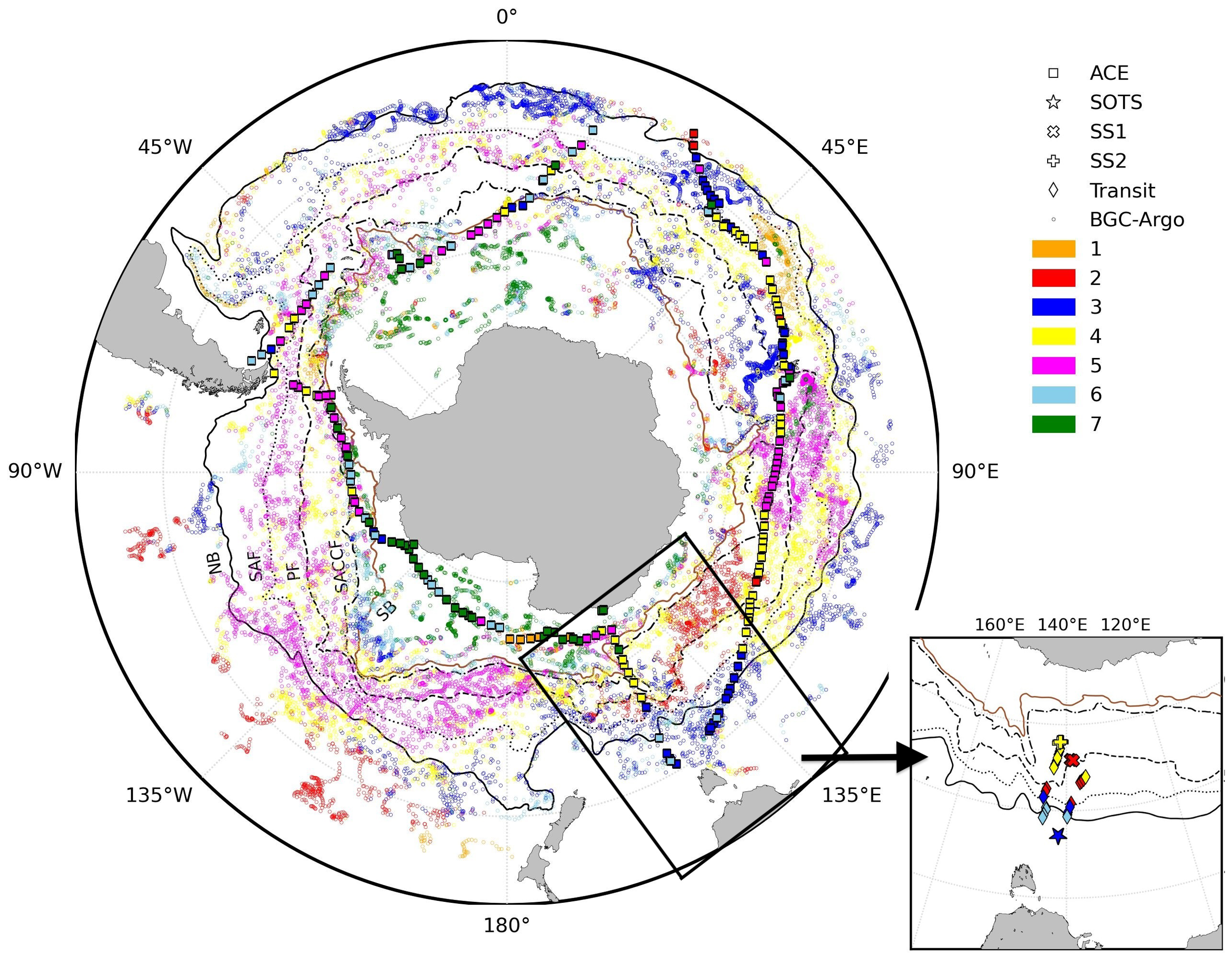
Sampling locations during ACE (squares) and SOLACE (SOTS, SS1, SS2, and transit sites, inset), as well as surface sampling points from BGC-Argo floats, colour-mapped according to the bioregions described in Ardyna et al. (2017). The Northern boundary (NB), Subantarctic Front (SF), Polar Front (PF), Southern Antarctic Circumpolar Current Front (SACCF), and Southern boundary (SB) from Park et al. (2019) are also displayed (black lines).
Measurements from both cruises and BGC-Argo floats were classified based on the seven bioregions defined by Ardyna et al. (2017) (Figure 2). This split aims to examine whether our dataset evenly samples various oceanographic regimes and to assess whether there are regional differences in the particulate bio-optical properties in addition to their large-scale patterns. The data from floats mostly fall into bioregions 3, 4, and 5, with only one-third belonging to the other bioregions. The distribution of cruise data is similar to that of float data, although high-latitude regions 6 and 7 are more prominently represented. Only average values from the top 10 m of the BGC-Argo data profiles are used in this work, combined with cruise data from underway sampling (depth ~5 m) and the top 10 m of data from CTD casts, as described in the following sections.
Figure 2
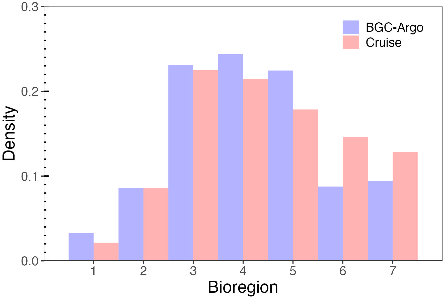
Distribution of cruise and float measurements among the seven bioregions defined by Ardyna et al. (2017).
The BGC-Argo profiling floats (https://biogeochemical-argo.org) used in this study, equipped with CTD and bio-optical sensors, measured temperature, salinity, pressure, chlorophyll fluorescence, and volume scattering (used to derive backscattering coefficient). Figure 1 shows the geographical location of all profiles collected by 254 floats from January 2016 to June 2023. The data points are colour-coded based on the bioregions in which the floats operated, following the regionalisation outlined by Ardyna et al. (2017).
2.2 Phytoplankton pigments and particulate absorption
Phytoplankton pigment concentrations from ACE and SOLACE were determined using high-performance liquid chromatography (HPLC, see details in Ras et al. (2008); Antoine et al. (2020) and references therein). On both cruises, 2.2 L water samples were collected either 3 hourly from the underway seawater supply (sampling depth ~ 5 m) or from the shallowest depth of the conductivity, temperature, and depth (CTD) rosette casts (see Table 1 for a summary of the number of samples). Total chlorophyll a concentration was defined as the sum of mono- and divinyl chlorophyll a concentrations, chlorophyllide a, and the allomeric and epimeric forms of chlorophyll a (Hooker and Zibordi, 2005; Reynolds et al., 2016).
Table 1
| Chl | bbp(λ) | ap(λ) | POC | PSD | |
|---|---|---|---|---|---|
| ACE | 221 | 13 | 274 | 355 | 264 |
| SOLACE | 31 | 3 | 31 | 3 | 3 |
| BGC-Argo floats | 21,872 | 21,872 | – | – | – |
Summary of the in situ dataset.
The pigments are used here to determine the relative contributions of micro- (fmicro, > 20 µm), nano- (fnano, 2–20 µm), and picophytoplankton (fpico, < 2 µm) to the total population, following Brewin et al. (2015).
For the BGC-Argo floats, the calibrated fluorescence profiles were adjusted for nonzero deep values (below 600 dbar) and corrected for spikes using a five-point median filter. Subsequently, they were divided by 3.79, as recommended by Schallenberg et al. (2022) for the SO. The surface Chl was obtained by averaging the values within the top 10 dbar.
A full description of the determination of the absorption coefficient of phytoplankton and non-algal particles (NAP) from the total particulate absorption coefficient can be found in Robinson et al. (2021), which is not repeated here.
2.3 Backscattering measurements
The particulate backscattering coefficient, bbp(λ) (m−1), was determined on ACE and SOLACE using HOBI Labs HydroScat-6 sensors, which provide a measurement of the total spectral volume scattering function β(ψ) (m−1 sr−1) at an effective scattering angle . The following equation (Maffione and Dana, 1997) was used to convert to bbp (λ),
Where the subscripts p and w indicate the contributions from particles and seawater to scattering, respectively. χ is the coefficient of proportionality between β and bb for particles, set to 1.13 for the HydroScat. Pure water values for at given temperature and salinity were calculated following Zhang et al. (2009). Finally, vertical profile data of bbp(λ) were filtered to remove spikes and averaged into 0.5 m depth bins for analysis and correlation with discrete water samples. The Hydroscat channels were 420 nm, 488 nm, 550 nm, 620 nm, and 700 nm for ACE (the 442 nm channel failed), and 420 nm, 442 nm, 470 nm, 510 nm, 590 nm, and 700 nm for SOLACE. For ACE, only 13 bbp spectra were obtained, primarily during leg 2 near the Antarctic continent.
To examine the wavelength dependency of particle backscattering, discrete spectral measurements were fitted to a power function of the following form:
Where λ0 represents a reference wavelength, and η denotes the dimensionless spectral slope of bbp. Nonlinear least-squares fitting was applied to account for bbp at all channels to derive η. Since the 442-nm spectral channel failed during the ACE cruise, this wavelength was excluded from the fitting of spectral relationships for the SOLACE cruise to ensure consistency between cruises.
Since our focus is on the total particle pool, we did not apply the nonzero deep value correction to the backscattering profile of BGC-Argo floats, as proposed by Uchida et al. (2019). This correction is meant to isolate the part of bbp attributed to phytoplankton by removing the average of deep values (below 600 dbar), which are assumed to represent the NAP contribution. We applied a five-point median filter to remove spikes (Carranza et al., 2018; Mignot et al., 2018). Surface values were obtained by averaging the data within the top 10 dbar of the profile.
2.4 Particulate organic carbon concentration
For the ACE dataset, the concentration of POC was obtained from the underway seawater supply every 3 h, as well as from several depths during the CTD rosette casts, and processed at the University of Cape Town (Fawcett and Forrer, 2020). Up to 2 L water samples were filtered through precombusted 25 mm GF/F filters. The filters were then dried at 40°C for 24 h, acidified to remove inorganic carbon, and stored until elemental analysis. Finally, POC for each sample was obtained by subtracting the average concentration of carbon in the dry blanks and was expressed in units of milligrammes per cubic metre. Samples outside the detection limits were eliminated. The same methodology was used for the SOLACE POC data, although it was processed at the University of Tasmania by Cathryn Wynn-Edwards.
2.5 Particle size distributions
The particle size distributions (PSD) determine their optical properties along with the particle composition. During ACE, PSD was measured with a Beckmann Coulter Counter Multisizer, which measures particle sizes by quantifying changes in electrical resistance produced by particles suspended in seawater as they pass through an aperture (Kinsman, 2018). In this study, 0.2 µm filtered seawater was used as the blank to detect particles in the range of 2–60 µm across 400 bins at each underway station. Twenty replicate measurements of 2 ml subsamples were made by the Counter for each sample and summed up to provide larger sample volumes, thereby improving statistical accuracy. Each discrete Coulter measurement included a set of values representing the particle concentrations (m−3) within a size bin D, N(D). The bin diameters were restricted to 2–30 µm, as no particles were observed in larger bins. Plots of particle concentration versus bin diameter were visually inspected, and samples with high noise levels or particle concentrations constrained to just a few bins were flagged as poor quality and removed (Robinson et al., 2021). Finally, 264 records of PSD were retained for further analysis.
During SOLACE, the PSD of large (> 100 μm) particles was measured using an Underwater Video Profiler 5 (UVP-5, Picheral et al., 2010) mounted on the rosette. Particle cross-sectional areas are quantified by assessing the contiguous pixels for a given image brightness level, which were then used to estimate the equivalent circular diameter. Finally, PSDs were determined for 24 bins, with centre bin sizes ranging from 115 to 23,300 µm. An upper limit of 2,315 µm was chosen to avoid regions of low particle counts and high statistical noise at large particle diameters. All data were binned vertically into 5-m intervals, and only surface values were used in this study.
The particle size distribution was fitted to a power law model (Bader, 1970; Jonasz and Fournier, 2011):
Where D0 is a reference diameter, N0 is the particle number at D0, and ζ is the dimensionless slope of the distribution. For the Coulter measurements, these metrics were calculated to characterize the samples and were computed over the size range of 4–20 µm. Since ζ is very sensitive to the range of effective diameters used and can be biased when an abundant phytoplankton cell size is present, leading to a bump on the PSD, we visually inspected the spectra and removed 15 spectra where clear bumps were present to avoid these cases.
2.6 Phytoplankton carbon estimations
C phyto is a key parameter in estimating primary production using various models (Sathyendranath et al., 2007). It also allows an understanding of phytoplankton physiology, as reflected in variations of cellular chlorophyll-to-carbon ratios generated by changes in light, temperature, and nutrients (Behrenfeld et al., 2005). However, Cphyto is difficult to distinguish experimentally in situ or in laboratory studies from the total carbon included in phytoplankton plus zooplankton, detritus, and bacteria. Consequently, direct Cphyto estimations are scarce, and essentially proxy measurements have been used to quantify it, such as Chl, cell biovolume, POC, and bbp.
Here, in the absence of direct Cphyto measurements, it was estimated using either the POC vs. Chl relationship or from bbp. The former approach assumes that at any given Chl, the lowest POC observed represents the phytoplankton fraction, Cphyto (Sathyendranath et al., 2009). In this approach, a 1% quantile regression is applied to the fit between POC and Chl to obtain Cphyto, hereafter denoted as Cphyto-S09. Since there will always be some contribution to POC from material other than phytoplankton, such as heterotrophs and detritus, this Cphyto estimate likely represents an upper limit for a given Chl. In addition, this approach does not allow for scenarios where Cphyto increases or decreases without a corresponding change in Chl (Thomalla et al., 2017). However, it is unlikely to be influenced by phenomena such as coccolith blooms or bubbles, which can significantly increase backscattering or the attenuation coefficient without increasing Chl.
Backscattering-based approaches allow Cphyto to vary independently of Chl, making them less susceptible to the package effect or photoacclimation. As a result, they are able to detect the high temporal variability in Chl:Cphyto ratios. These methods assume Cphyto is linearly related to bbp. Behrenfeld et al. (2005) established such a relationship by fitting satellite-derived bbp (440) to which a background value of 3.5 × 10⁻⁴ m−1 is subtracted to laboratory Cphyto values:
which is denoted as Cphyto-B05 hereafter. The subtraction of the background value accounts for the portion of backscattering attributed to a background of NAP that does not covary with phytoplankton.
Based on direct measurements of both Cphyto and bbp in the Atlantic Ocean, Martinez-Vicente et al. (2013) found a significant linear relationship between Cphyto and bbp(470) (denoted as Cphyto-M13):
This linear regression was initially limited to bbp (470) < 0.003 m−1 or Chl < 0.4 mg m−3; however, in this study, we extended it for the larger Chl range as well.
Using data from the Equatorial Pacific Ocean and from the 22nd Atlantic Meridional Transect cruise, Graff et al. (2015) established yet another relationship:
Hereafter denoted as Cphyto-G15.
Note that, for backscatter measurements lacking a 440- or 470-nm channel, the values at 700 nm were converted to these other wavelengths using Equation 2, with η equal to 1.08 (mean of the measured values).
3 Results and discussions
3.1 General latitudinal distribution of properties
The latitudinal distribution of average values of major environment parameters and inherent optical properties (IOPs) is presented in Figure 3. These values are calculated from all data found in 2° latitude bands centred on latitudes from 40°S to 74°S. Hereafter, Chl and bbp are measured both through ship-based hydrographic casts and BGC-Argo floats are denoted separately as Chl-Cruise and Chl-Float (and bbp-Cruise and bbp-Float).
Figure 3
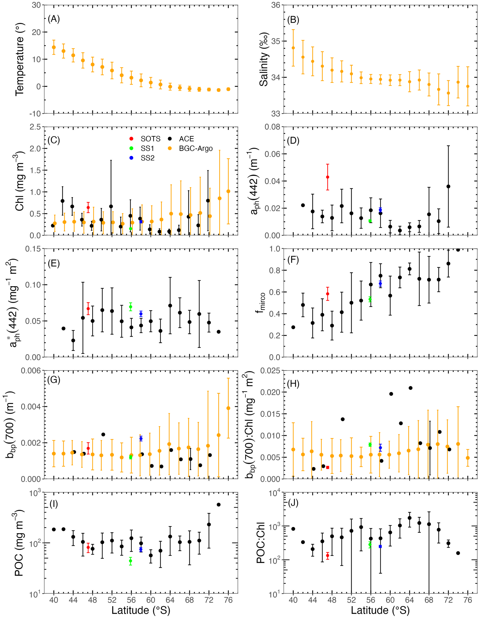
Latitudinal distribution of (A) temperature, (B) salinity, (C) Chl, (D)aph(442), (E), (F)fmicro, (G)bbp(700), (H)bbp(700) to Chl ratio, (I) POC, and (J) POC to Chl ratio. Black symbols represent measurements made from hydrographic casts on ships, while orange symbols refer to BGC-Argo float measurements. The red, blue, and green dots refer to the SOTS, SS1, and SS2 sites, respectively. Data were grouped into 2° latitude intervals, within which the mean values and standard deviations were calculated.
Temperature decreases toward the south (Figure 3A), from about 15°C at 40°S to − 1°C close to the Antarctic continent. Salinity also shows a general decreasing trend toward the south (Figure 3B), with two relative maxima observed around 65°S and near the continent.
Minima of Chl-Cruise are found around 60°S~68°S and maxima around 45°S and 72°S (Figure 3C). The Chl-Cruise and Chl-Float are quite consistent, with the differences mainly due to the uneven cruise sampling. In the 41°S~45°S latitudinal belt, Chl-Cruise measurements were constrained in the area south of the African continent and are higher than Chl-Float. In the 59°S to 67°S latitudinal belt, Chl-Cruise was at the lowest level (< 0.2 mg m−3) at the Drake Passage and the Dumont d’Urville Sea. As for the 69°S~76°S latitudinal belt, Chl-Float measurements are higher than Chl-Cruise and have larger variance because they were collected in more varied environments. Among the SOLACE data, Chl-Cruise is the highest at SOTS with a mean value of 0.64 mg m−3, followed by SS2 (0.31 mg m−3) and SS1 (0.15 mg m−3).
The latitudinal distribution of aph(442) (Figure 3D) reflects that of Chl-Cruise, yet shows a smaller relative increase toward high latitudes, leading to a decrease of the chlorophyll-specific absorption coefficient at 442 nm, (Figure 3E).
The fraction of larger phytoplankton, fmicro, increases from about 0.3 to 0.9 toward the south (Figure 3F), which is consistent with the findings by Robinson et al. (2021).
Generally, bbp (700) (Figure 3G) is quite stable in the 40 to 60°S belt, with a mean value of ~ 0.0012 m−1. South of 60°S, the mean values and associated variance both increase. The 16 bbp-Cruise all fall within the range of the bbp-Float values. Due to the very limited bbp measurements on cruises, they were excluded from further analyses with respect to the large-scale latitudinal analyses. The mean bbp:Chl ratios across latitudes (Figure 3H) fluctuate between 0.005 and 0.008 m2 mg−1.
The POC (Figure 3I) varies between 30 and 200 mg m−3, with minimum values around 60°S and an average value of 105 mg m−3 across the dataset. The POC:Chl ratio (Figure 3J) varies over one order of magnitude, from 100 to 1,000, and shows relative maxima around 54°S and 64°S, with a regular decrease for latitude south of about 64°S.
It is worth noting that BGC-Argo data from all seasons have been pooled together here, whereas the cruise data are for the summer months only (December to February, plus early March for ACE). If Figure 3 was to include BGC-Argo data for only the 3 summer months, the only two notable differences would be the slightly higher bbp(700) values (0.002 instead of 0.0015 m−1 on average for latitudes above 70°S) and, similarly, the slightly higher Chl for latitudes above 60°S (with an average of approximately 0.4 instead of 0.25 mg m−3). The discrepancy between Chl-Cruise and Chl-Float would be reinforced in the 60°S–68°S band, primarily due to the ship sampling being restricted to the Drake Passage and Dumont d’Urville Sea.
When the zonal averages displayed in Figure 3 are restricted to the Atlantic, Indian, and Pacific sectors, the latter displays the lowest Chl (average 0.2 mg m−3). In contrast, the subtropical latitudes of the Indian Ocean are saltier (salinity ~ 35 psu), warmer (SST up to 17°C), and have the largest POC concentrations (around 100 mg m−3). No other major differences are observed among the three sectors and between the results for each sector and those for the entire SO.
3.2 Bio-optical relationships
The various bio-optical relationships we have explored are illustrated in Figure 4. The ratio of NAP to phytoplankton absorption, (Figure 4A), shows an upward tail in low Chl waters (Chl < 0.2 mg m−3), with values larger than 1 and as large as 10. For larger Chl values (> 0.2 mg m−3), the ratio slowly decreases as Chl increases. This result not only suggests a high contribution of NAP, such as heterotrophs and detritus, to the particle pool in clear waters of the SO, but also that this contribution is highly variable.
Figure 4
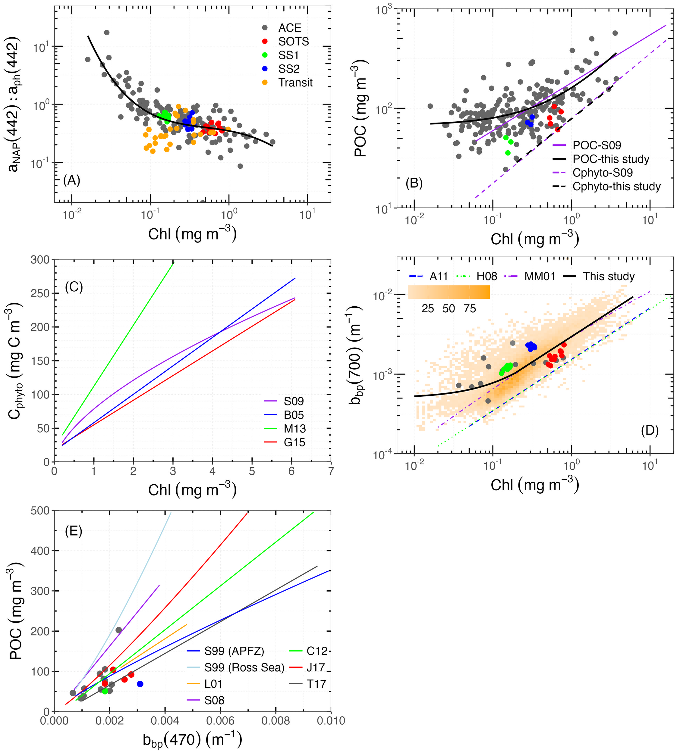
Bio-optical relationships. (A) aNAP:aph ratio at 442 nm vs. Chl. The black solid line represents the fourth-degree polynomial regression in log space for our dataset, . (B) POC vs. Chl. The black solid curve represents . The dashed black line represents the 1% quantile regression on the same data, representing the relationship between Cphyto and Chl (), following Sathyendranath et al. (2009). The purple solid and dashed lines refer to the POC vs. Chl and Cphyto vs. Chl relationships from Sathyendranath et al. (2009), respectively. (C) Cphyto vs. Chl. See Section 2.6 for S09, B05, M13, and G15. (D) bbp(700) vs. Chl. The background orange symbols refer to the density of float measurements. The solid black line represents the regression line between bbp(700) and Chl, using both ship and float data from this study: (Chl ≤ 0.2 mg m−3); (Chl > 0.2 mg m−3). The blue, green, and purple lines refer to the relationships from Antoine et al. (2011) in the Northwestern Mediterranean Sea and Santa Barbara Channel, Huot et al. (2008) in the Eastern South Pacific Ocean, and Morel and Maritorena (2001) for global oceanic waters, respectively. (E) POC vs. bbp(470). S99, L01, S08, C12, J17, and T17 refer to the relationships from Stramski et al. (1999) in the Antarctic Polar Front Zone (APFZ) and the Ross Sea, Loisel et al. (2001) in the Mediterranean Sea, Stramski et al. (2008) in the Pacific and Atlantic Oceans, Cetinić et al. (2012) in the North Atlantic Ocean, Johnson et al. (2017) in the SO, and Thomalla et al. (2017) in the South Atlantic and SO, respectively. Note that for models without bbp at 470 nm, values were propagated from other available bands according to Equation 2 using .
This large contribution of NAP to the particle pool in the SO seems corroborated by the POC vs. Chl relationship (Figure 4B). Here, Chl-Cruise varies over nearly three orders of magnitude, and POC over two, and their relationship shows the generally expected increasing trend but only for Chl > 0.2 mg m−3. Below this concentration, POC fluctuates around 80 mg m−3, independent of Chl levels, again suggesting that NAP significantly contributes to POC in the clear waters of the SO.
The POC vs. Chl relationship is generally expressed through a linear fit on log-transformed data. For instance, Sathyendranath et al. (2009) found such a linear relationship () using data from the equatorial Pacific and Atlantic Oceans, denoted POC-S09 hereafter (solid purple line in Figure 4B). In our study, a linear regression in log space is not appropriate to describe the POC vs. Chl relationship because of the relatively constant POC in waters where Chl is less than 0.2 mg m−3, attributed to the contribution of NAP to POC. Therefore, we added a constant background POC in our linear regression. When a linear fit without constant background value is applied to data for Chl > 0.2 mg m−3 only, the obtained POC vs. Chl relationship shows no significant difference with POC-S09.
We also applied 1% quantile regression on the data where Chl > 0.2 mg m−3 to derive Cphyto, following the approach of Sathyendranath et al. (2009), resulting in a remarkably similar relationship (dashed and solid purple lines in Figure 4B). By converting bbp-Float to Cphyto according to Behrenfeld et al. (2005); Martinez-Vicente et al. (2013), and Graff et al. (2015), Cphyto vs. Chl can be obtained as well, denoted as B05, M13 and G15, respectively. Their comparison with S09 is illustrated in Figure 4C. The slope of M13 is significantly higher than the others, resulting in a difference up to 160 mg m−3 in Cphyto at Chl = 3 mg m−3. B05 and G15 have similar intercepts, although the slope of B05 is slightly higher. Their largest difference is about 50 mg m−3 in Cphyto at Chl = 6 mg m−3. S09 generally derives higher Cphyto per Chl, while G15 intersects with B05 at Chl = 4.3 mg m−3, with their differences in Cphyto remaining within 50 mg m−3 across all Chl ranges.
B05 and M13 assume a constant background bbp due to NAP (denoted bbp-NAP) that does not covary with phytoplankton. However, Bellacicco et al. (2016) found that bbp-NAP varies both seasonally and regionally by more than one order of magnitude, which might result in significant errors in the Cphyto estimates. G15 is the only one using analytical field-measured Cphyto, which has been found to have a significant correlation with bbp in the Equatorial Pacific Ocean and Atlantic Ocean.
None of these methods (either Chl or bbp-based) have been derived using data collected in the SO, so their applicability here cannot be ascertained. Their consistent Cphyto prediction is however encouraging. It is still worth noting that the aforementioned approaches do not seem applicable to waters with Chl < 0.2 mg m−3, due to the high NAP contribution to the particle pool. The substantial contribution of NAP to POC and bbp further complicates the accurate estimation of Cphyto in such waters. Therefore, sufficient concurrent measurements of phytoplankton community composition and their specific chlorophyll and carbon content are needed to evaluate and validate optical methods of determining Cphyto concentrations, and then to assess Chl: Cphyto ratios for better understanding phytoplankton physiology under environmental forcing.
The bbp-Cruise and bbp-Float data are displayed as a function of Chl in Figure 4D. The former varies between 0.0004 and 0.004 m−1 in the combined ACE and SOLACE dataset, and all fall within the larger range (0.0002~0.1 m−1) measured by floats over the entire SO. Values obtained during SOLACE were generally higher than those observed during ACE leg 2 near the Antarctic continent. The highest values were obtained at SS2 with the smallest variation, followed by those at SOTS and SS1. The spectral slope of bbp(λ), calculated using all available wavebands, fluctuates from 0.5 to 1.6, with a mean value of 1.08. The bbp-Float values generally increase with Chl, although they remain relatively constant in the low Chl range (again, Chl < 0.2 mg m−3). For Chl > 0.2 mg m−3, bbp covaries with Chl, which is consistent with previous observations (Antoine et al., 2011; Bellacicco et al., 2019). Therefore, we here combined a linear regression for Chl < 0.2 mg m−3 with a power law for Chl > 0.2 mg m−3 to fit the data (solid black curve in Figure 4D).
For comparison, other relationships obtained from in situ data collected in the Northwestern Mediterranean Sea and Santa Barbara Channel by Antoine et al. (2011) (denoted A11) and in the Eastern South Pacific Ocean by Huot et al. (2008) (denoted M08) are also shown. For A11, their bbp(560) was converted to bbp(700) according to Equation 2. The bbp(700) vs. Chl relationship from Morel and Maritorena (2001) (denoted MM01) developed for the oceanic case I waters is shown as well. Generally, the bbp(700) of MM01 is significantly higher than H08 and A11 across the Chl range, which might be due to the difference in study regions. For Chl > 0.2 mg m−3, our fit generally coincides with MM01, but with a slightly larger slope. For Chl < 0.2 mg m−3, bbp(700) is higher than predicted by MM01, with differences that can reach up to one order of magnitude. The high contribution of NAP is likely responsible for these larger bbp values in clear waters as compared to what global models predict from Chl. Such relative constant bbp is likely a consequence of the combination of photoacclimation and the high proportion of NAP. The former is typical for polar waters, where Chl variation is driven by photoacclimation to low light and thus uncoupled with biomass, leading to an increase of Chl without a corresponding increase in bbp (Behrenfeld et al., 2005; Brewin et al., 2012; Bellacicco et al., 2019).
It is also worth noting that we did not find significant differences among bbp-Float vs. Chl-Float relationships as separately derived for each Ardyna’s bioregions.
The ACE and SOLACE datasets have only 16 concurrent measurements of POC and bbp(470). They are shown in Figure 4E on top of relationships obtained from both temperate oceans and subregion of the SO (see figure caption for details). There is a large spread of POC vs. bbp(470) relationships across different regions. The highest POC: bbp(470) statistical mean ratio is noticed in the Ross Sea, while the lowest is also found in the SO from 20°W ~ 20°E by Thomalla et al. (2017). In addition, their difference in POC is about 350 mg m−3 at bbp(470) = 0.004 m−1 and continues to increase as bbp increases. Thus, there is no clear POC vs. bbp relationship in the SO, especially for high-scattering waters. This lack of correlation is due to the contributions of both POC and particulate inorganic carbon (PIC) to backscattering.
It appears that in the SO, we cannot use a single linear regression to describe the relationships of bio-optical properties and chlorophyll over the full concentration range. For Chl < 0.2 mg m−3, the large NAP contribution tends to mask any possible phytoplankton-related changes in bio-optical properties.
3.3 Particle size distributions
PSD of surface waters measured by the Coulter Counter and UVP-5 are illustrated in Figure 5. Particle concentrations (m−3 μm−1) decrease when the equivalent spherical diameter increases and generally follow a Junge-type size distribution. This is expected, yet exceptions occur, with peaks appearing at certain diameters, e.g., 10 μm, which may indicate phytoplankton blooms dominated by a particular size group. Although the Coulter and UVP-5 use different approaches to determine particle size, cross-sectional area for the UVP-5, and particle volume for the Coulter Counter, the slopes determined over different size ranges are quite similar (a mean value of 3.99 for Coulter Counter data and 4.29 for UVP-5 data). Among the SOLACE data, the number of particles is overall larger at SS1 and SS2 than at SOTS, although the latter displays a larger Chl. This observation of more large particles (UVP-5 data start at 100 µm) at the two clearer southern sites seems consistent with the larger NAP contribution already identified for the domain of smaller particles.
Figure 5
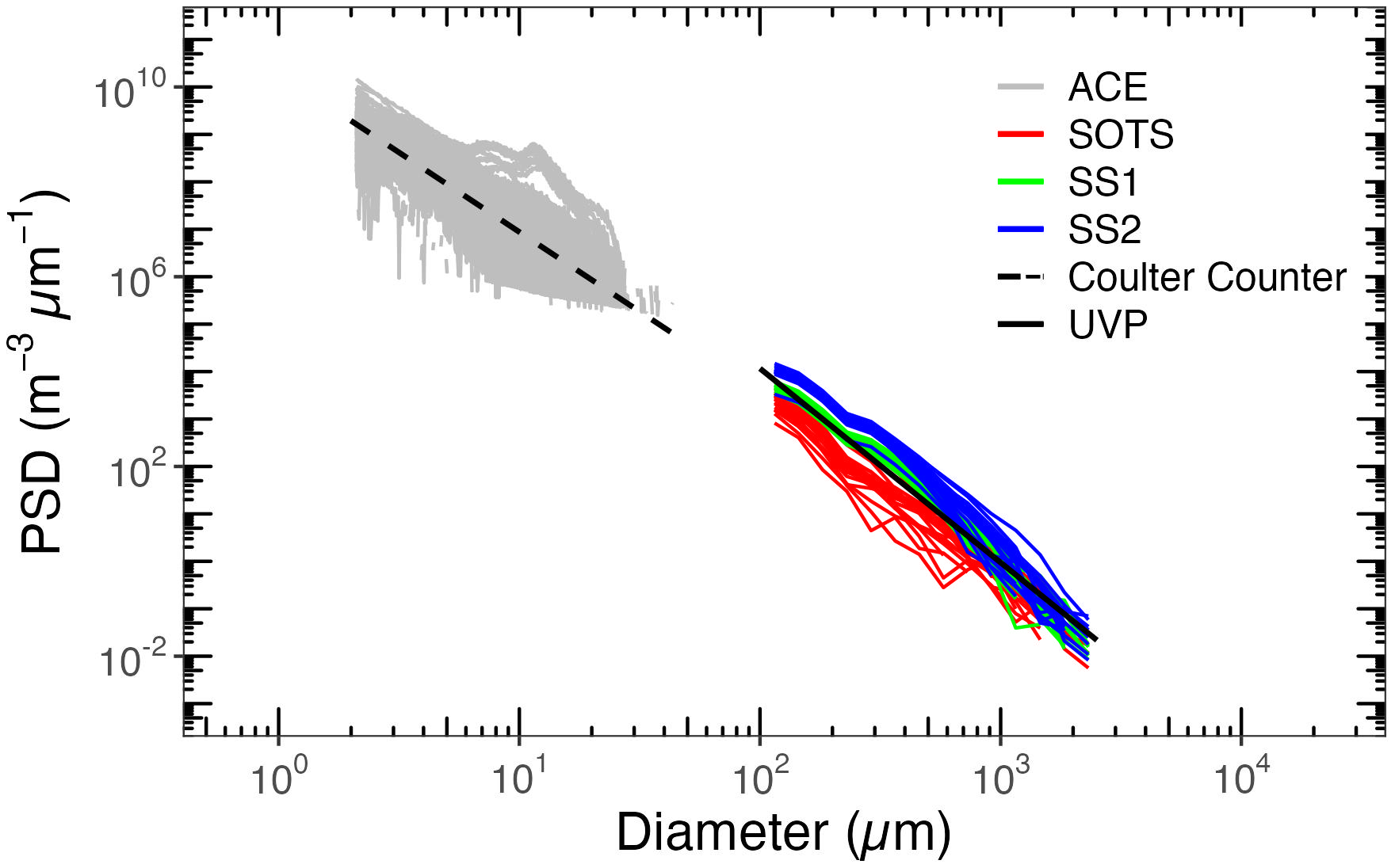
Particle size distributions derived from Coulter Counter and UVP-5.
PSD slopes (ζ, unitless) are displayed as a function of Chl, colour-mapped as a function of the fraction of microphytoplankton (fmicro) derived according to Brewin et al. (2015) (Figure 6). The slope ζ varies between 3 and 5. A somewhat decreasing trend can be discerned for Chl > 0.2 mg m−3, similar to what Buonassissi and Dierssen (2010) have found in temperate regions, yet there is no significant relationship when Chl appears below 0.2 mg m−3, suggesting the particle distribution is heterogenous within the SO. In addition, we did not notice a clear impact of fmicro on ζ. The expectation would be that populations dominated by larger cells would have a lower ζ, which is not clearly observed here.
Figure 6
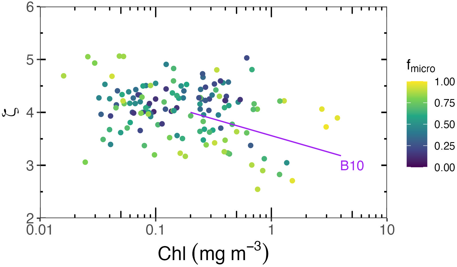
PSD slope ζ vs. Chl relationship. The dots are colour-mapped as a function of the fraction of micro-phytoplankton derived from Brewin et al. (2015). The purple line represents the relationship obtained by Buonassissi and Dierssen (2010) in the North Atlantic, where .
3.4 Implications for ocean colour remote sensing
The absorption of NAP follows an exponential decay from the blue to the red parts of the spectrum. In the clear waters we have analysed here (Chl < 0.2 mg m−3), the large NAP contribution leads to significant non-chlorophyll absorption in the blue part of the spectrum (λ < ~ 500 nm). A likely consequence is a lower blue-to-green remote-sensing reflectance band ratio than would otherwise exist for the same Chl concentration but with a lower NAP contribution. This would result in a significant overestimation of Chl when using global empirical ocean colour algorithms to derive Chl from the reflectance ratio, as the NAP absorption would be wrongly interpreted as phytoplankton absorption.
To verify this, we compared in situ Chl from both cruise and float measurements with satellite-derived Chl estimates. For this purpose, we used the Moderate Resolution Imaging Spectroradiometer (MODIS) L3b binned chlorophyll products, which use a sinusoidal projection so that each grid cell covers the same area, regardless of latitude. For each in situ measurement covered by a product, a 3 × 3 window centred on the in situ location was extracted. In total, we found 311 in situ and satellite-derived Chl matchups, which are displayed in Figure 7.
Figure 7
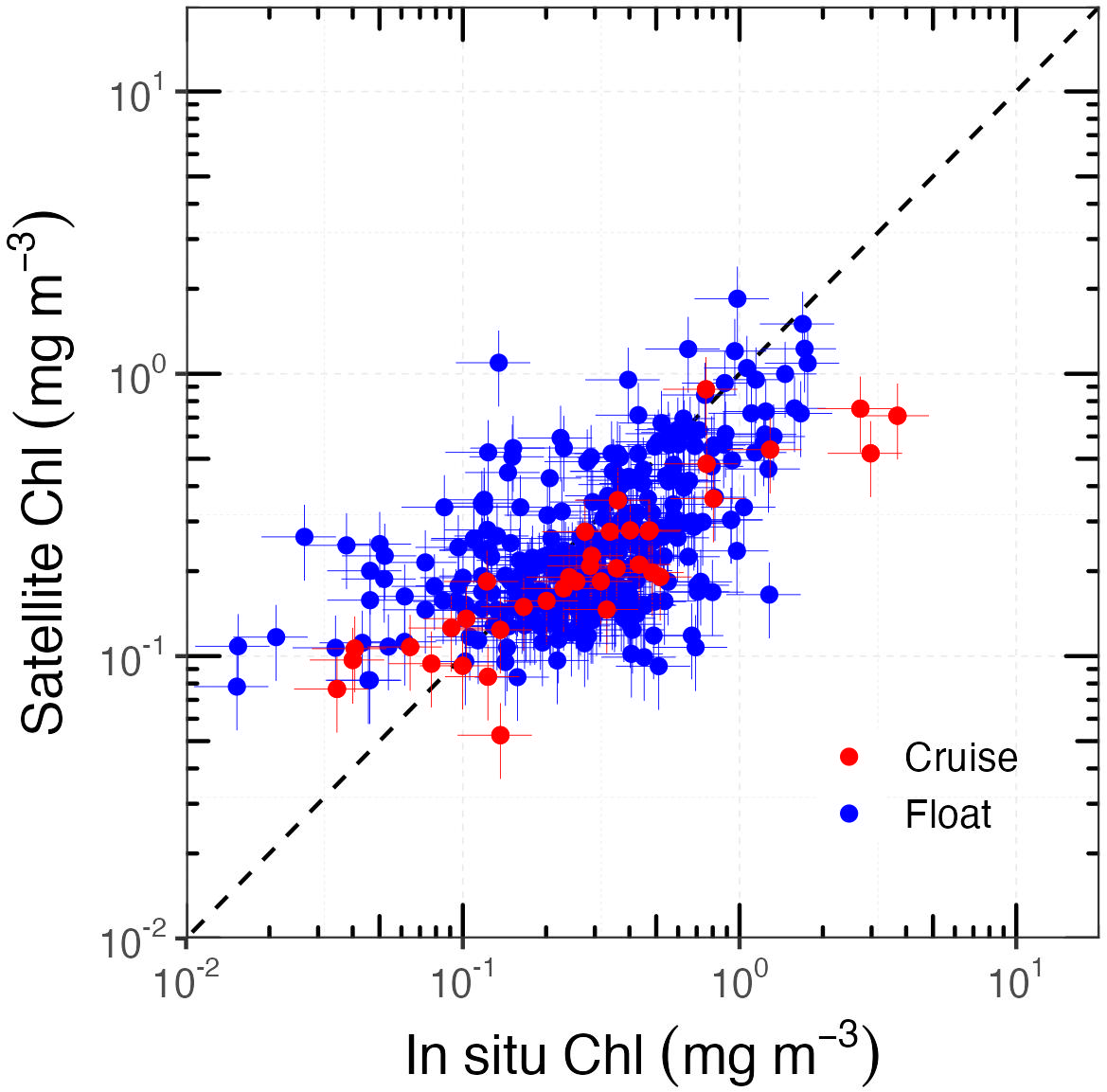
Comparisons between in situ and satellite-derived Chl. The black dashed line represents the 1:1 relationship. Error bars indicate the typical 30% uncertainty for both the HPLC- and satellite-derived Chl.
Previous similar matchup studies generally reported an underestimation of Chl by satellite products in the SO (Garcia et al., 2005; Marrari et al., 2006; Kahru and Mitchell, 2010; Szeto et al., 2011; Johnson et al., 2013; Jena, 2017; Pereira and Garcia, 2018; Moutier et al., 2019). This is confirmed here, but only for Chl > 0.2 mg m−3. For lower values, we conversely observe an overestimation. This is consistent with the excess NAP absorption reported here. It cannot be ruled out, however, that larger absorption by coloured dissolved organic matter (CDOM) would also contribute to this overestimation of Chl (Morel and Gentili, 2009). The absence of reflectance measurements from the ACE and SOLACE voyages did not allow these hypotheses to be further tested here.
4 Conclusions
By combining ship-based measurements from the ACE and SOLACE research voyages and profiling-float-based measurements from over 20,000 profiles collected by the BGC-Argo network, we were able to analyse the general latitudinal distribution patterns of particle-related bio-optical and biogeochemical variables, as well as the associated bio-optical relationships.
At latitudes beyond 60°S, Chl, aph, bbp, POC, and fmicro increase toward the Antarctic continent. In parallel, the chlorophyll-normalised values of aph and POC decrease, while the chlorophyll-specific bbp remains stable across latitudes.
The absorption data showed a high proportion of NAP (aNAP:aph up to 10) in the clear waters (Chl < 0.2 mg m−3) of the SO. This substantial NAP contribution leads to higher POC and bbp values, making particulate bio-optical properties significantly different from what is expected for temperate areas. In contrast, this divergence is not evident in waters with Chl > 0.2 mg m−3. Therefore, using bio-optical relationships developed in temperate waters to study the SO is probably acceptable outside the domain of low Chl. The specific relationships we propose here (Figure 4) are presumably better adapted to the SO. Nonetheless, caution is warranted, as even minor alterations in these relationships can result in notable absolute differences due to the substantial variability present.
The implication for satellite ocean colour applications seems to be an overestimation of Chl in clear waters when using standard algorithms (again, in areas with Chl levels below 0.2 mg m−3). Deriving better SO-adapted Chl retrieval algorithms that account for this peculiarity would, however, require more comprehensive datasets of bio-optical properties and radiometry measurements, which still do not exist at the required scale. This is definitely where more effort should be directed if we are to expect significant improvements in our ability to monitor SO ecosystems from space.
Statements
Data availability statement
Publicly available datasets were analyzed in this study. This data can be found here: BGC-Argo float data is available at https://biogeochemical-argo.org. Data collected during cruises is available at https://zenodo.org/records/3993096, https://doi.org/10.5281/zenodo.3816726, https://doi.org/10.5281/zenodo.3660852, https://doi.org/10.5281/zenodo.3706710.
Author contributions
JL: Conceptualization, Data curation, Formal analysis, Investigation, Methodology, Software, Validation, Visualization, Writing – original draft, Writing – review & editing. DA: Conceptualization, Data curation, Funding acquisition, Resources, Supervision, Writing – review & editing. YH: Conceptualization, Methodology, Supervision, Visualization, Writing – review & editing.
Funding
The author(s) declare financial support was received for the research, authorship, and/or publication of this article. JL was supported by the Australian Research Council Special Research Initiative, Australian Centre for Excellence in Antarctic Science (ACEAS; Project Number SR200100008). ACE was funded by Ferring Pharmaceuticals with additional support from the Swiss Polar Institute. Funding from the Australian Research Council Discovery Program (DP160103387) contributed to the exploitation of ACE data.
Acknowledgments
We would like to thank all members of the ACE Project, including Charlotte Robinson, William Moutier, David Berliner, Alexandra Olivier, and Hazel Little, as well as staff from the Swiss Polar Institute and the crew from the RV Akademik Trynoshnikov. SOLACE received support from the Australian Government through ship time at the Marine National Facility (MNF; R/V Investigator). We thank the scientific staff and crew of the R/V Investigator for facilitating work at the three SOLACE sites in the Southern Ocean.
Conflict of interest
The authors declare that the research was conducted in the absence of any commercial or financial relationships that could be construed as a potential conflict of interest.
Publisher’s note
All claims expressed in this article are solely those of the authors and do not necessarily represent those of their affiliated organizations, or those of the publisher, the editors and the reviewers. Any product that may be evaluated in this article, or claim that may be made by its manufacturer, is not guaranteed or endorsed by the publisher.
References
1
Allison D. B. Stramski D. Mitchell B. G. (2010a). Empirical ocean color algorithms for estimating particulate organic carbon in the Southern Ocean. J. Geophysical Research: Oceans115. doi: 10.1029/2009JC006040
2
Allison D. B. Stramski D. Mitchell B. G. (2010b). Seasonal and interannual variability of particulate organic carbon within the Southern Ocean from satellite ocean color observations. J. Geophysical Research: Oceans115. doi: 10.1029/2009JC005347
3
Antoine D. Siegel D. A. Kostadinov T. Maritorena S. Nelson N. B. Gentili B. et al . (2011). Variability in optical particle backscattering in contrasting bio-optical oceanic regimes. Limnology Oceanography56, 955–973. doi: 10.4319/lo.2011.56.3.0955
4
Antoine D. Thomalla S. Berliner D. Little H. Moutier W. Olivier-Morgan A. et al . (2020). Phytoplankton pigment concentrations of seawater sampled during the Antarctic Circumnavigation Expedition (ACE) during the Austral Summer of 2016/2017. doi: 10.5281/zenodo.3816726
5
Ardyna M. Claustre H. Sallée J.-B. D’Ovidio F. Gentili B. van Dijken G. et al . (2017). Delineating environmental control of phytoplankton biomass and phenology in the Southern Ocean. Geophysical Res. Lett.44, 5016–5024. doi: 10.1002/2016GL072428
6
Arrigo K. R. van Dijken G. L. Bushinsky S. (2008). Primary production in the southern ocean 1997–2006. J. Geophysical Research: Oceans113. doi: 10.1029/2007JC004551
7
Bader H. (1970). The hyperbolic distribution of particle sizes. J. Geophysical Res.75, 2822–2830. doi: 10.1029/JC075i015p02822
8
Behrenfeld M. J. Boss E. Siegel D. A. Shea D. M. (2005). Carbon-based ocean productivity and phytoplankton physiology from space. Global Biogeochem. Cycles.19. doi: 10.1029/2004GB002299
9
Belcher A. Iversen M. Manno C. Henson S. A. Tarling G. A. Sanders R. (2016). The role of particle associated microbes in remineralization of fecal pellets in the upper mesopelagic of the Scotia Sea, Antarctica. Limnology Oceanography61, 1049–1064. doi: 10.1002/lno.10269
10
Bellacicco M. Cornec M. Organelli E. Brewin R. J. W. Neukermans G. Volpe G. et al . (2019). Global variability of optical backscattering by non-algal particles from a biogeochemical-argo data set. Geophysical Res. Lett.46, 9767–9776. doi: 10.1029/2019GL084078
11
Bellacicco M. Volpe G. Colella S. Pitarch J. Santoleri R. (2016). Influence of photoacclimation on the phytoplankton seasonal cycle in the Mediterranean Sea as seen by satellite. Remote Sens. Environ.184, 595–604. doi: 10.1016/j.rse.2016.08.004
12
Boyd P. W. Claustre H. Levy M. Siegel D. A. Weber T. (2019). Multi-faceted particle pumps drive carbon sequestration in the ocean. Nature568, 327–335. doi: 10.1038/s41586-019-1098-2
13
Boyd P. W. McDonnell A. Valdez J. LeFevre D. Gall M. P. (2015). RESPIRE: An in situ particle interceptor to conduct particle remineralization and microbial dynamics studies in the oceans’ Twilight Zone. Limnology Oceanography: Methods13, 494–508. doi: 10.1002/lom3.10043
14
Brewin R. J. W. Dall’Olmo G. Sathyendranath S. Hardman-Mountford N. J. (2012). Particle backscattering as a function of chlorophyll and phytoplankton size structure in the open-ocean. Opt. Express20, 17632–17652. doi: 10.1364/OE.20.017632
15
Brewin R. J. W. Sathyendranath S. Jackson T. Barlow R. Brotas V. Airs R. et al . (2015). Influence of light in the mixed-layer on the parameters of a three-component model of phytoplankton size class. Remote Sens. Environ.168, 437–450. doi: 10.1016/j.rse.2015.07.004
16
Briggs N. Dall’Olmo G. Claustre H. (2020). Major role of particle fragmentation in regulating biological sequestration of CO 2 by the oceans. Science367, 791–793. doi: 10.1126/science.aay1790
17
Buesseler K. O. Lamborg C. H. Boyd P. W. Lam P. J. Trull T. W. Bidigare R. R. et al . (2007). Revisiting carbon flux through the ocean’s twilight zone. Science316, 567–570. doi: 10.1126/science.1137959
18
Buonassissi C. J. Dierssen H. M. (2010). A regional comparison of particle size distributions and the power law approximation in oceanic and estuarine surface waters. J. Geophys. Res.115, C10028. doi: 10.1029/2010JC006256
19
Carranza M. M. Gille S. T. Franks P. J. S. Johnson K. S. Pinkel R. Girton J. B. (2018). When mixed layers are not mixed. Storm-driven mixing and bio-optical vertical gradients in mixed layers of the southern ocean. J. Geophysical Research: Oceans123, 7264–7289. doi: 10.1029/2018JC014416
20
Cavan E. L. Trimmer M. Shelley F. Sanders R. (2017). Remineralization of particulate organic carbon in an ocean oxygen minimum zone. Nat. Commun.8, 14847. doi: 10.1038/ncomms14847
21
Cetinić I. Perry M. J. Briggs N. T. Kallin E. D’Asaro E. A. Lee C. M. (2012). Particulate organic carbon and inherent optical properties during 2008 North Atlantic Bloom Experiment. J. Geophysical Research: Oceans117. doi: 10.1029/2011JC007771
22
Clements D. J. Yang S. Weber T. McDonnell A. M. P. Kiko R. Stemmann L. et al . (2022). Constraining the particle size distribution of large marine particles in the global ocean with in situ optical observations and supervised learning. Global Biogeochemical Cycles36, e2021GB007276. doi: 10.1029/2021GB007276
23
Falkowski P. G. Barber R. T. Smetacek V. (1998). Biogeochemical controls and feedbacks on ocean primary production. Science281, 200–206. doi: 10.1126/science.281.5374.200
24
Fawcett S. Forrer H. (2020). Particulate organic carbon concentration in seawater profiles collected on board the R/V Akademik Tryoshnikov in the Southern Ocean during the austral summer of 2016/2017 as part of the Antarctic Circumnavigation Expedition (ACE). Zenodo. doi: 10.5281/zenodo.3706710
25
Garcia C. A. E. Garcia V. M. T. McClain C. R. (2005). Evaluation of SeaWiFS chlorophyll algorithms in the Southwestern Atlantic and Southern Oceans. Remote Sens. Environ.95, 125–137. doi: 10.1016/j.rse.2004.12.006
26
Graff J. R. Westberry T. K. Milligan A. J. Brown M. B. Dall’Olmo G. Dongen-Vogels V. et al . (2015). Analytical phytoplankton carbon measurements spanning diverse ecosystems. Deep Sea Res. Part I: Oceanographic Res. Papers102, 16–25. doi: 10.1016/j.dsr.2015.04.006
27
Gruber N. Gloor M. Mikaloff Fletcher S. E. Doney S. C. Dutkiewicz S. Follows M. J. et al . (2009). Oceanic sources, sinks, and transport of atmospheric CO2. Global Biogeochemical Cycles23. doi: 10.1029/2008GB003349
28
Hirawake T. Takao S. Horimoto N. Ishimaru T. Yamaguchi Y. Fukuchi M. (2011). A phytoplankton absorption-based primary productivity model for remote sensing in the Southern Ocean. Polar Biol.34, 291–302. doi: 10.1007/s00300-010-0949-y
29
Hooker S. B. Zibordi G. (2005). Advanced methods for characterizing the immersion factor of irradiance sensors. J. Atmos. Oceanic Technol.22, 757–770. doi: 10.1175/JTECH1736.1
30
Huot Y. Morel A. Twardowski M. S. Stramski D. Reynolds R. A. (2008). Particle optical backscattering along a chlorophyll gradient in the upper layer of the eastern South Pacific Ocean. Biogeosciences5, 495–507. doi: 10.5194/bg-5-495-2008
31
Jackson G. A. (1980). Phytoplankton growth and Zooplankton grazing in oligotrophic oceans. Nature284, 439–441. doi: 10.1038/284439a0
32
Jackson G. A. Burd A. B. (1998). Aggregation in the marine environment. Environ. Sci. Technol.32, 2805–2814. doi: 10.1021/es980251w
33
Jena B. (2017). The effect of phytoplankton pigment composition and packaging on the retrieval of chlorophyll-a concentration from satellite observations in the Southern Ocean. Int. J. Remote Sens.38, 3763–3784. doi: 10.1080/01431161.2017.1308034
34
Johnson K. S. Plant J. N. Coletti L. J. Jannasch H. W. Sakamoto C. M. Riser S. C. et al . (2017). Biogeochemical sensor performance in the SOCCOM profiling float array. J. Geophysical Research: Oceans122, 6416–6436. doi: 10.1002/2017JC012838
35
Johnson R. Strutton P. G. Wright S. W. McMinn A. Meiners K. M. (2013). Three improved satellite chlorophyll algorithms for the Southern Ocean. J. Geophysical Research: Oceans118, 3694–3703. doi: 10.1002/jgrc.20270
36
Jonasz M. Fournier G. R. (2011). Light Scattering by Particles in Water: Theoretical and Experimental Foundations. (Elsevier). doi: 10.1016/B978-0-12-388751-1.X5000-5
37
Kahru M. Mitchell B. G. (2010). Blending of ocean colour algorithms applied to the Southern Ocean. Remote Sens. Lett.1, 119–124. doi: 10.1080/01431160903547940
38
Karakuş O. Völker C. Iversen M. Hagen W. Hauck J. (2022). The role of zooplankton grazing and nutrient recycling for global ocean biogeochemistry and phytoplankton phenology. J. Geophysical Research: Biogeosciences127, e2022JG006798. doi: 10.1029/2022JG006798
39
Kinsman S. (2018). “Particle Size Instrumentation — Coulter® Counter,” in Particle Characterization in Technology. Ed. BeddowJ. K. (Boca Raton: CRC Press), 183–186. doi: 10.1201/9781351075350-9
40
Loisel H. Bosc E. Stramski D. Oubelkheir K. Deschamps P.-Y. (2001). Seasonal variability of the backscattering coefficient in the Mediterranean Sea based on satellite SeaWiFS imagery. Geophysical Res. Lett.28, 4203–4206. doi: 10.1029/2001GL013863
41
Maffione R. A. Dana D. R. (1997). Instruments and methods for measuring the backward-scattering coefficient of ocean waters. Appl. Optics36, 6057–6067. doi: 10.1364/AO.36.006057
42
Marrari M. Hu C. Daly K. (2006). Validation of SeaWiFS chlorophyll a concentrations in the Southern Ocean: A revisit. Remote Sens. Environ.105, 367–375. doi: 10.1016/j.rse.2006.07.008
43
Martinez-Vicente V. Dall’Olmo G. Tarran G. Boss E. Sathyendranath S. (2013). Optical backscattering is correlated with phytoplankton carbon across the Atlantic Ocean. Geophys. Res. Lett.40, 1154–1158. doi: 10.1002/grl.50252
44
Mignot A. Ferrari R. Claustre H. (2018). Floats with bio-optical sensors reveal what processes trigger the North Atlantic bloom. Nat. Commun.9, 190. doi: 10.1038/s41467-017-02143-6
45
Morel A. Gentili B. (2009). A simple band ratio technique to quantify the colored dissolved and detrital organic material from ocean color remotely sensed data. Remote Sens. Environ.113, 998–1011. doi: 10.1016/j.rse.2009.01.008
46
Morel A. Maritorena S. (2001). Bio-optical properties of oceanic waters: A reappraisal. J. Geophys. Res.106, 7163–7180. doi: 10.1029/2000JC000319
47
Moutier W. Thomalla S. Bernard S. Wind G. Ryan-Keogh T. Smith M. (2019). Evaluation of chlorophyll-a and POC MODIS aqua products in the southern ocean. Remote Sens.11, 1793. doi: 10.3390/rs11151793
48
Park Y.-H. Park T. Kim T.-W. Lee S.-H. Hong C.-S. Lee J.-H. et al . (2019). Observations of the antarctic circumpolar current over the udintsev fracture zone, the narrowest choke point in the southern ocean. J. Geophysical Research: Oceans124, 4511–4528. doi: 10.1029/2019JC015024
49
Pereira E. S. Garcia C. A. E. (2018). Evaluation of satellite-derived MODIS chlorophyll algorithms in the northern Antarctic Peninsula. Deep Sea Res. Part II: Topical Stud. Oceanography149, 124–137. doi: 10.1016/j.dsr2.2017.12.018
50
Picheral M. Guidi L. Stemmann L. Karl D. M. Iddaoud G. Gorsky G. (2010). The Underwater Vision Profiler 5: An advanced instrument for high spatial resolution studies of particle size spectra and zooplankton. Limnology Oceanography: Methods8, 462–473. doi: 10.4319/lom.2010.8.462
51
Ras J. Claustre H. Uitz J. (2008). Spatial variability of phytoplankton pigment distributions in the Subtropical South Pacific Ocean: comparison between in situ and predicted data. Biogeosciences5, 353–369. doi: 10.5194/bg-5-353-2008
52
Reynolds R. A. Stramski D. Neukermans G. (2016). Optical backscattering by particles in Arctic seawater and relationships to particle mass concentration, size distribution, and bulk composition: Particle backscattering in Arctic seawater. Limnol. Oceanogr61, 1869–1890. doi: 10.1002/lno.10341
53
Robinson C. M. Huot Y. Schuback N. Ryan-Keogh T. J. Thomalla S. J. Antoine D. (2021). High latitude Southern Ocean phytoplankton have distinctive bio-optical properties. Opt. Express29, 21084–21112. doi: 10.1364/OE.426737
54
Roesler C. Uitz J. Claustre H. Boss E. Xing X. Organelli E. et al . (2017). Recommendations for obtaining unbiased chlorophyll estimates from in situ chlorophyll fluorometers: A global analysis of WET Labs ECO sensors. Limnology Oceanography: Methods15, 572–585. doi: 10.1002/lom3.10185
55
Sarmiento J. L. Johnson K. S. Arteaga L. A. Bushinsky S. M. Cullen H. M. Gray A. R. et al . (2023). The Southern Ocean carbon and climate observations and modeling (SOCCOM) project: a review. Prog. Oceanogr.219, 103130. doi: 10.1016/j.pocean.2023.103130
56
Sathyendranath S. Platt T. Forget M.-H. (2007). “Oceanic Primary Production: Comparison of Models,” in OCEANS 2007. (Europe, Aberdeen, UK. (IEEE), 1–3. doi: 10.1109/OCEANSE.2007.4302468
57
Sathyendranath S. Stuart V. Nair A. Oka K. Nakane T. Bouman H. et al . (2009). Carbon-to-chlorophyll ratio and growth rate of phytoplankton in the sea. Mar. Ecol. Prog. Ser.383, 73–84. doi: 10.3354/meps07998
58
Schallenberg C. Harley J. W. Jansen P. Davies D. M. Trull T. W. (2019). Multi-year observations of fluorescence and backscatter at the southern ocean time series (SOTS) shed light on two distinct seasonal bio-optical regimes. Front. Mar. Sci.6. doi: 10.3389/fmars.2019.00595
59
Schallenberg C. Strzepek R. F. Bestley S. Wojtasiewicz B. Trull T. W. (2022). Iron limitation drives the globally extreme fluorescence/chlorophyll ratios of the southern ocean. Geophysical Res. Lett.49, e2021GL097616. doi: 10.1029/2021GL097616
60
Slade W. H. Boss E. Russo C. (2011). Effects of particle aggregation and disaggregation on their inherent optical properties. Opt. Express19, 7945–7959. doi: 10.1364/OE.19.007945
61
Stark J. S. Raymond T. Deppeler S. L. Morrison A. K. (2019). “Chapter 1 - Antarctic Seas,” in World Seas: an Environmental Evaluation (Second Edition). Ed. SheppardC. (Cambridge, Massachusetts: Academic Press), 1–44. doi: 10.1016/B978-0-12-805068-2.00002-4
62
Steinberg D. K. Landry M. R. (2017). Zooplankton and the ocean carbon cycle. Annu. Rev. Mar. Sci.9, 413–444. doi: 10.1146/annurev-marine-010814-015924
63
Stramska M. Stramski D. Hapter R. Kaczmarek S. Stoń-Egiert J. (2003). Bio-optical relationships and ocean color algorithms for the north polar region of the Atlantic. J. Geophys. Res.108, 3143. doi: 10.1029/2001JC001195
64
Stramski D. Reynolds R. A. Babin M. Kaczmarek S. Lewis M. R. Röttgers R. et al . (2008). Relationships between the surface concentration of particulate organic carbon and optical properties in the eastern South Pacific and eastern Atlantic Oceans. Biogeosciences5, 171–201. doi: 10.5194/bg-5-171-2008
65
Stramski D. Reynolds R. A. Kahru M. Mitchell B. G. (1999). Estimation of particulate organic carbon in the ocean from satellite remote sensing. Science285, 239–242. doi: 10.1126/science.285.5425.239
66
Szeto M. Werdell P. J. Moore T. S. Campbell J. W. (2011). Are the world’s oceans optically different? J. Geophysical Research: Oceans116. doi: 10.1029/2011JC007230
67
Thomalla S. J. Ogunkoya A. G. Vichi M. Swart S. (2017). Using optical sensors on gliders to estimate phytoplankton carbon concentrations and chlorophyll-to-carbon ratios in the southern ocean. Front. Mar. Sci.4. doi: 10.3389/fmars.2017.00034
68
Turner J. T. (2015). Zooplankton fecal pellets, marine snow, phytodetritus and the ocean’s biological pump. Prog. Oceanography130, 205–248. doi: 10.1016/j.pocean.2014.08.005
69
Uchida T. Balwada D. Abernathey R. Prend C. J. Boss E. Gille S. T. (2019). Southern ocean phytoplankton blooms observed by biogeochemical floats. J. Geophysical Research: Oceans124, 7328–7343. doi: 10.1029/2019JC015355
70
Walton D. W. H. Thomas J. (2018). Cruise report - antarctic circumnavigation expedition (ACE) 20th december 2016 - 19th march 2017. doi: 10.5281/zenodo.1443511
71
Wynn-Edwards C. Davies D. M. Jansen P. Bray S. G. Eriksen R. Trull T. W. (2019). IMOS-Southern Ocean Time Series (SOTS)-Annual Reports: 2012/2013. (Australian Integrated Marine Observing System, University of Tasmania).
72
Zhang Y. L. Liu M. L. Wang X. Zhu G. W. Chen W. M. (2009). Bio-optical properties and estimation of the optically active substances in Lake Tianmuhu in summer. Int. J. Remote Sens.30, 2837–2857. doi: 10.1080/01431160802558592
Summary
Keywords
Southern Ocean, particles, bio-optical properties, bio-optical relationships, BGC-Argo floats
Citation
Li J, Antoine D and Huot Y (2024) Bio-optical variability of particulate matter in the Southern Ocean. Front. Mar. Sci. 11:1466037. doi: 10.3389/fmars.2024.1466037
Received
17 July 2024
Accepted
24 September 2024
Published
23 October 2024
Volume
11 - 2024
Edited by
Jianchuan Yin, Guangdong Ocean University, China
Reviewed by
Sarat Chandra Tripathy, National Centre for Polar and Ocean Research (NCPOR), India
Guifen Wang, Hohai University, China
Updates
Copyright
© 2024 Li, Antoine and Huot.
This is an open-access article distributed under the terms of the Creative Commons Attribution License (CC BY). The use, distribution or reproduction in other forums is permitted, provided the original author(s) and the copyright owner(s) are credited and that the original publication in this journal is cited, in accordance with accepted academic practice. No use, distribution or reproduction is permitted which does not comply with these terms.
*Correspondence: David Antoine, david.antoine@curtin.edu.au
Disclaimer
All claims expressed in this article are solely those of the authors and do not necessarily represent those of their affiliated organizations, or those of the publisher, the editors and the reviewers. Any product that may be evaluated in this article or claim that may be made by its manufacturer is not guaranteed or endorsed by the publisher.