Abstract
Orcinus orca (killer whales) exhibit complex calls. In a call, an orca typically varies the frequencies, varies the length, varies the temporal patterns, varies their volumes, and can use multiple frequencies simultaneously. Behavior data is hard to obtain because orcas live under water and travel quickly. Sound data is relatively easy to capture. This paper studies whether machine learning can predict behavior from vocalizations. Such prediction would help scientific research and have safety applications because one would like to predict behavior while only having to capture sound. A significant challenge in this process is lack of labeled data. This paper works with recent recordings of McMurdo Sound orcas where each recording is labeled with the behaviors observed during the recording. This yields a dataset where sound segments—continuous vocalizations that can be thought of as call sequences or more general structures—within the recordings are labeled with potentially superfluous behaviors. This is because in a given segment, an orca may not be exhibiting all of the behaviors that were observed during the recording from which the segment was taken. Despite that, with a careful combination of recent machine learning techniques, including a ResNet-34 convolutional neural network and a custom loss function designed for partially labeled learning, a 96.1% general behavior label classification accuracy on previously unheard segments is achieved. This is promising for future research on orca behavior as well as language and safety applications.
1 Introduction
Marine biologists have recordings of Orcinus orca (killer whale) vocalizations in which they have identified what they coin “calls” [e.g., Poupard et al. (2021)]. Generally speaking, calls fall into two categories, whistles or pulsed calls, and are used for communication (Ford, 1989, 1991). These calls are variable in length and can be classified into discrete call types according to temporal patterns, fundamental frequency, and duration, among other features (Wellard et al., 2020a; Ford, 1989). Even within an individual call, an orca varies the frequencies, varies their volumes, and can use multiple frequencies simultaneously, as in the case of biphonic calls (Filatova, 2020; Ford, 1989).In addition, orcas produce echolocation clicks which they use to observe their surroundings (Ford, 1989; Schevill and Watkins, 1966; Leu et al., 2022).
Researchers have clustered orca calls into 4 to 91 call types depending on the study. The call types likely depend on the population studied (Schröter et al., 2019; Wellard et al., 2020a; Ford et al., 2011; Ford, 1991, 1989; Schall and Van Opzeeland, 2017; Selbmann et al., 2023). For example, the fish-eating resident orcas in the Pacific Northwest have sets of calls that are pod-specific (Ford, 1984, 1991, 1989). Those orcas form pods that are stable matriarchal social groups (Ford, 1989). The set of calls such a pod uses is called its vocal repertoire. It consist of 7 to 17 call types (Ford, 1991). Such pods have different but overlapping vocal repertoires, and they have pod-specific ways of “pronouncing” calls, which together form the pod’s “dialect” (Ford, 1991). Orcas in Iceland have a vocal repertoire of up to 91 calls (Selbmann et al., 2023). The orcas studied in this paper, the Type C orcas in the Ross Sea, have been found to have 28 call types (Wellard et al., 2020a).
Past studies have found certain links between orca vocalizations and behavior. For example, Icelandic orcas have been observed using low-frequency pulsed calls to scare Atlantic Herring into schools before using tail slaps to immobilize, and subsequently feed on, the herring (Simon et al., 2006). Additionally, the different dialects of the resident orcas of the North Pacific are also highly connected to the social activity and development of the resident matrilines (Filatova et al., 2012; Deecke et al., 2000; Weiß et al., 2007; Yurk et al., 2002; Miller and Bain, 2000). Ford (1989) found that certain calls, namely variable, aberrant, and discrete calls, may be used as social calls by the resident orcas of the Pacific Northwest. Weiß et al. (2006) found that the resident orcas of the North Pacific use more of their unique pod-specific calls for several weeks after the birth of a calf. Weiß et al. (2006) theorize this shift in vocal behavior is an effort to get the calf to learn the pod-specific calls. However, there is still little understanding of what these calls convey (Schröter et al., 2019). This is because orcas live underwater and move quickly, making it difficult for researchers to record the orcas with a camera. Thus, the sound recordings are rarely accompanied by other data that would support such reasoning.
While the types of calls used by orcas have been extensively studied, it is still quite difficult to determine an orca’s behavior from vocalization data alone. I aim to develop a machine learning-based software system that makes it easier to determine orca behavior from vocalization data. I use a recent orca sound recording collection that is rare in the sense that it includes auxiliary data about the orcas’ behaviors (Wellard et al., 2020b, a). I segment these recordings to isolate continuous orca vocalizations that are typically many times as long as individual calls. In a segment, the orcas may not be exhibiting all of the behaviors that were observed during the recording from which the segment was taken. This yields a data set where the segments are labeled with potentially superfluous behaviors. This presents a significant problem: a lack of fully labeled behavior data. I use a custom loss function which is designed for learning on partially labeled data to combat this issue (Feng et al., 2020). By carefully combining and tailoring select modern machine learning techniques, I show that sound segments—call sequences or even more general structures—can be used to predict orca behavior with 96.1% accuracy (although classification accuracy varied considerably among behavioral categories). Since the data is partially labeled, accuracy is determined based on the general behavior labels. The model’s performance concerning the actual behavior or behaviors shown in a given segment cannot be assessed.
To my knowledge, this paper is the first to use partially labeled learning to study animal vocalizations and the first to use machine learning to analyze orca sound segments beyond individual calls. Prior research on whale sounds has primarily focused on identifying whales in passive acoustic listening and identifying individual call types. For example, Bergler et al. (2019a) used unsupervised learning to cluster orca calls. Bergler et al. (2019b) worked on classifying orca calls using a ResNet-18 neural network.1Deecke et al. (1999) used a neural network to analyze the differences in the calls of different orca dialects. Bergler et al. (2019c) created a system using convolutional neural networks that can differentiate orca calls from environmental noise. Beyond orcas, studies involving the identification of certain species of whale with vocalization data using machine learning have been conducted on false killer whales (Murray et al., 1998), sperm whales (Jiang et al., 2018; Bermant et al., 2019; Andreas et al., 2022), long-finned pilot whales (Jiang et al., 2018), right whales (Shiu et al., 2020), beluga whales (Zhong et al., 2020), fin whales (Best et al., 2022), humpback whales (Allen et al., 2021), and blue whales (Miller et al., 2022). Also, the PAMGUARD software has been developed to identify cetacean presence in passive acoustic listening data (Gillespie et al., 2009).
The recent sound recordings of Wellard et al. (2020b, a) that I use last between 51 seconds and 41 minutes each, for a total of 3.42 hours of recordings of Type C Ross Sea orcas from the McMurdo Sound in Antarctica. The Type C orca is a primarily fish-eating ecotype of the Southern Hemisphere orcas (Pitman and Ensor, 2003). However, Pitman and Ensor (2003) note that there have been speculative reports of Type C orcas hunting penguins and seals. Wellard et al. labeled each recording with all the orca behaviors that they observed during that recording: (T) for traveling, (F) for foraging, (S) for socializing, and (M) for milling/resting. Each recording can therefore have a combination of behavior labels. (Wellard et al. also identified different types of calls in that dataset. The shortest call type was on average 0.19 seconds long and the longest was on average 1.81 seconds long.)
2 Materials and methods
2.1 Sound preprocessing pipeline
Wellard et al. collected the recordings on the McMurdo Sound in Antarctica using a hydrophone. The recordings were in a.wav format. The recordings had a sampling rate of 96kHz with a bandwidth of 48 kHz or a sampling rate of 44.1 kHz with a bandwidth of 22.05 kHz. They recorded the orcas nine times throughout December, 2012 and January, 2013. The number of individuals sighted during each of the nine encounters can be seen in Table 1. There were two days, January 8 and January 11, where the orcas were recorded at two separate locations on the same day. Wellard et al. (2020a) also documented which call types were observed during each of the nine encounters2.
Table 1
| Date | Label combination | No. of sound segments | No. of individuals present | Duration |
|---|---|---|---|---|
| 12/26/2012 | {F, S} | 49 | 65 | 22:54.4 |
| 12/29/2012 | {F, S} | 73 | 19 | 26:44.6 |
| 01/03/2013 | {T, S} | 30 | 31 | 06:46.9 |
| 01/04/2013 | {T, F, S, M} | 19 | 63 | 05:34.9 |
| 01/08/2013 | {T, F} | 71 | 6 | 22:06.2 |
| 01/08/2013 | {T} | 76 | 7 | 15:16.4 |
| 01/09/2013 | {T, F, M} | 112 | 46 | 47:36.3 |
| 01/11/2013 | {T, S, F, M} | 16 | 59 | 13:03.3 |
| 01/11/2013 | {T} | 48 | 21 | 53:08.0 |
Date, behavior labels, numbers of sound segments, number of individuals sited by Wellard et al. (2020a), and duration (minutes:seconds) of recording for each of the nine encounters.
I accessed the recordings through the Dryad Digital Repository (Wellard et al., 2020b). These recordings ranged from 51 seconds to 41 minutes long. Based on the four possible behavior labels in the data— traveling (T), foraging (F), socializing (S), and milling/resting (M)—the recordings could in principle have any one of the 24 − 1 = 15 possible label combinations. However, in reality each recording had one of the following six label combinations: {T}, {F, S}, {T, S}, {T, F}, {T, F, M}, or {T, F, S, M}. The raw data files in the database are not labeled directly with their behavior labels. Instead, they are labeled with dates and no finer-grained information such as time stamps of the recordings. I extrapolated the data labels associated with each recording by comparing the behaviors observed on each recording day and the date labels on the sound files (Wellard et al., 2020b).
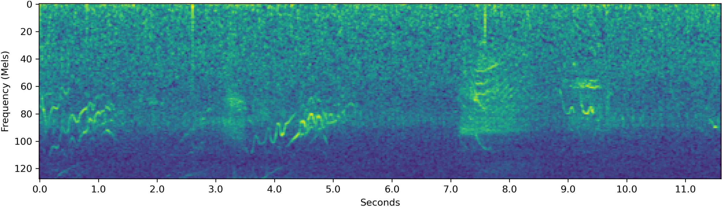
At the heart of my study is the analysis of sound segments—call sequences or even more general structures—not just individual calls. For this purpose, I segmented the recordings to create the sound segments for analysis by my system. Figure 1 shows two examples of segments and the recording from which they originated.
Figure 1
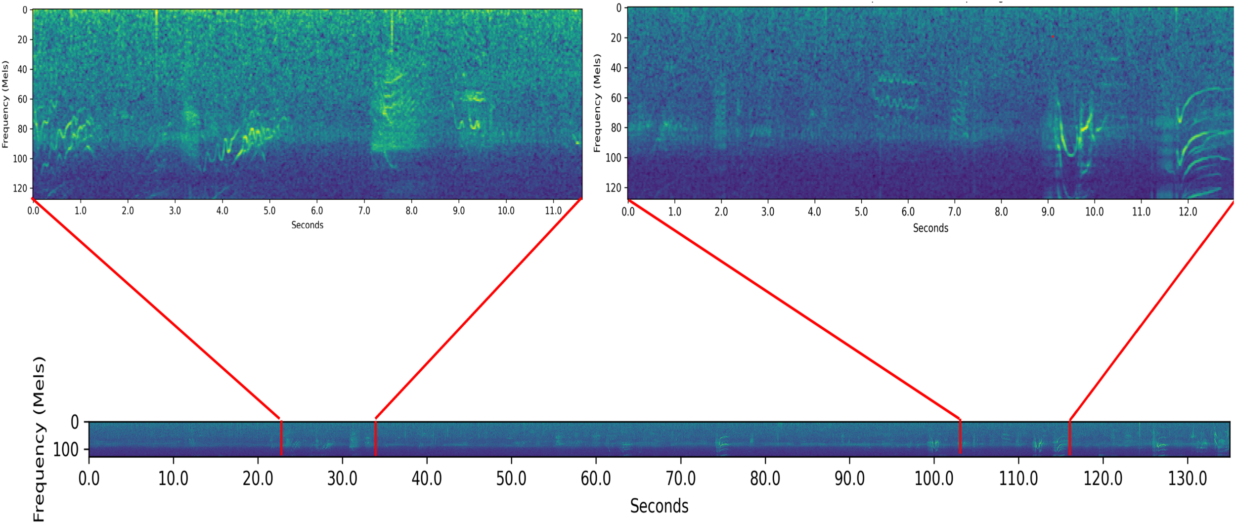
Examples of two segments contained within a sample recording. The bottom spectrogram is a 135 second long portion of a 5 minute and 15 second long recording from Wellard et al. This recording had the behavior label {T}. The two spectrograms at the top of the diagram are two segments contained within the recording. These segments’ places within the recording are marked in red.
I conducted the segmentation manually using an audio software called Audacity (version 3.4.2) to view the spectrograms of the recording and used the following rules to define a segment.
-
Each segment had to be longer than half a second.
-
Each segment had to occur at least two seconds apart from other segments. If vocalizations occurred less than two seconds apart, I considered them part of the same segment.
-
The orca vocalizations in any segment needed to be seen on the spectrogram in Audacity and be audible when played back at full volume on a laptop speaker3.
Criterion 1 was chosen to be half a second to make sure that the network would have enough data in each segment based on which to classify. Criterion 2 was chosen with the intention of capturing sequences of calls, as opposed to singular calls, while making sure that there was not a large gap between vocalizations. If these criteria were changed, there would be potential for a decreased amount of data, as is the case for loosening Criterion 2, as well as decreased data quality, as is the case for changing Criterion 1.
The numbers of sound segments after segmentation, with their associated label combinations, are shown in Table 2. Additionally, Table 1 shows the number of segments originating from each of the nine encounters and their associated behavior labels. The segments’ lengths ranged from 0.5 to 82.7 seconds and the mean length was 7.4 seconds. Segments of length 0.5 to 0.6 seconds, of which there were 144 in my dataset, consisted of one to two calls. The segments with a length of around 8.0 seconds all had at least five and at most 11 calls. An example of one such segment in .wav format can be seen in Figure 2a.
Table 2
| Label combination | Number of sound segments |
|---|---|
| {T} | 124 |
| {F, S} | 122 |
| {T, S} | 30 |
| {T, F} | 71 |
| {T, F, M} | 112 |
| {T, F, S, M} | 35 |
| Total | 494 |
Numbers of sound segments with the various label combinations.
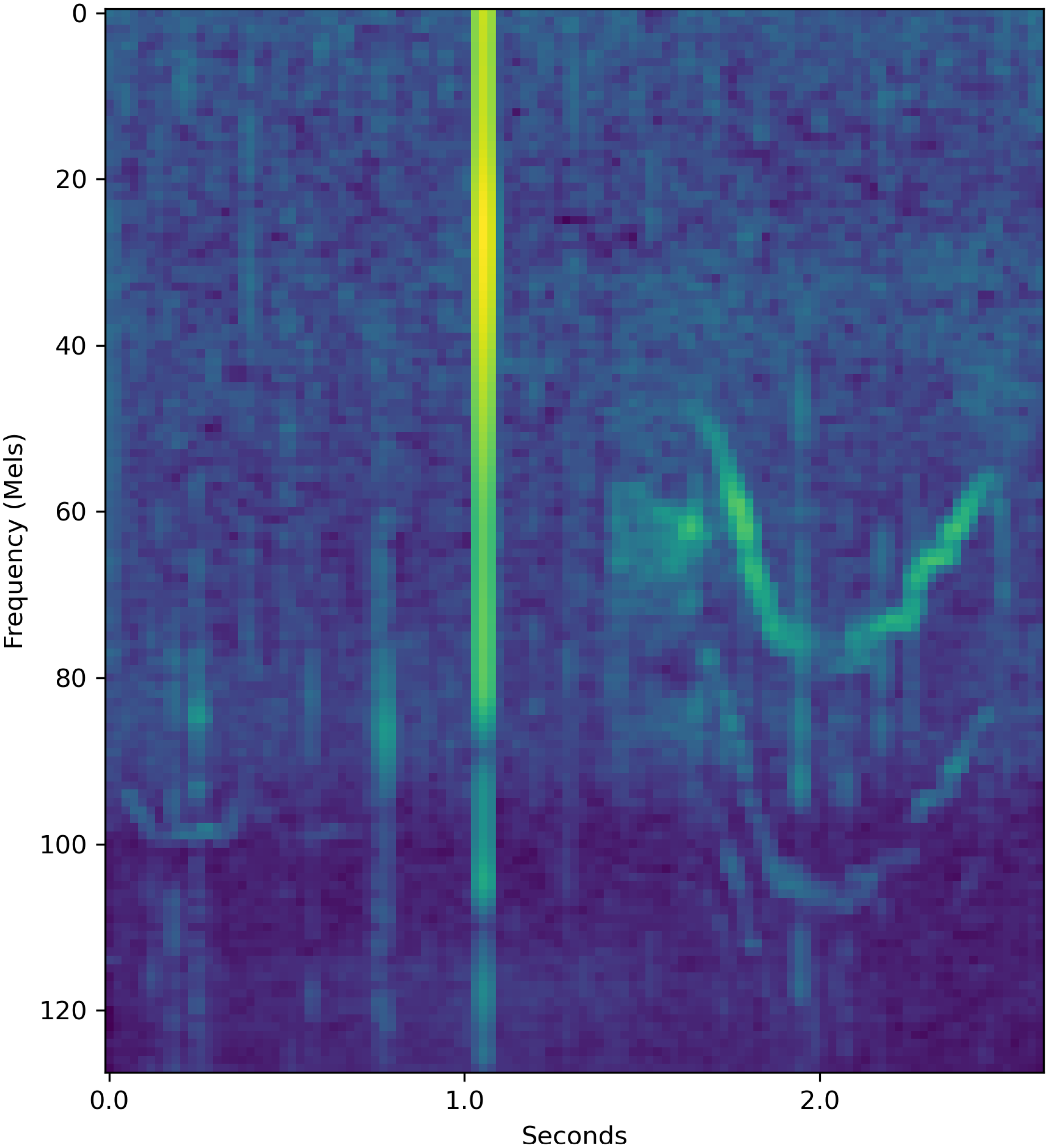
Figure 2
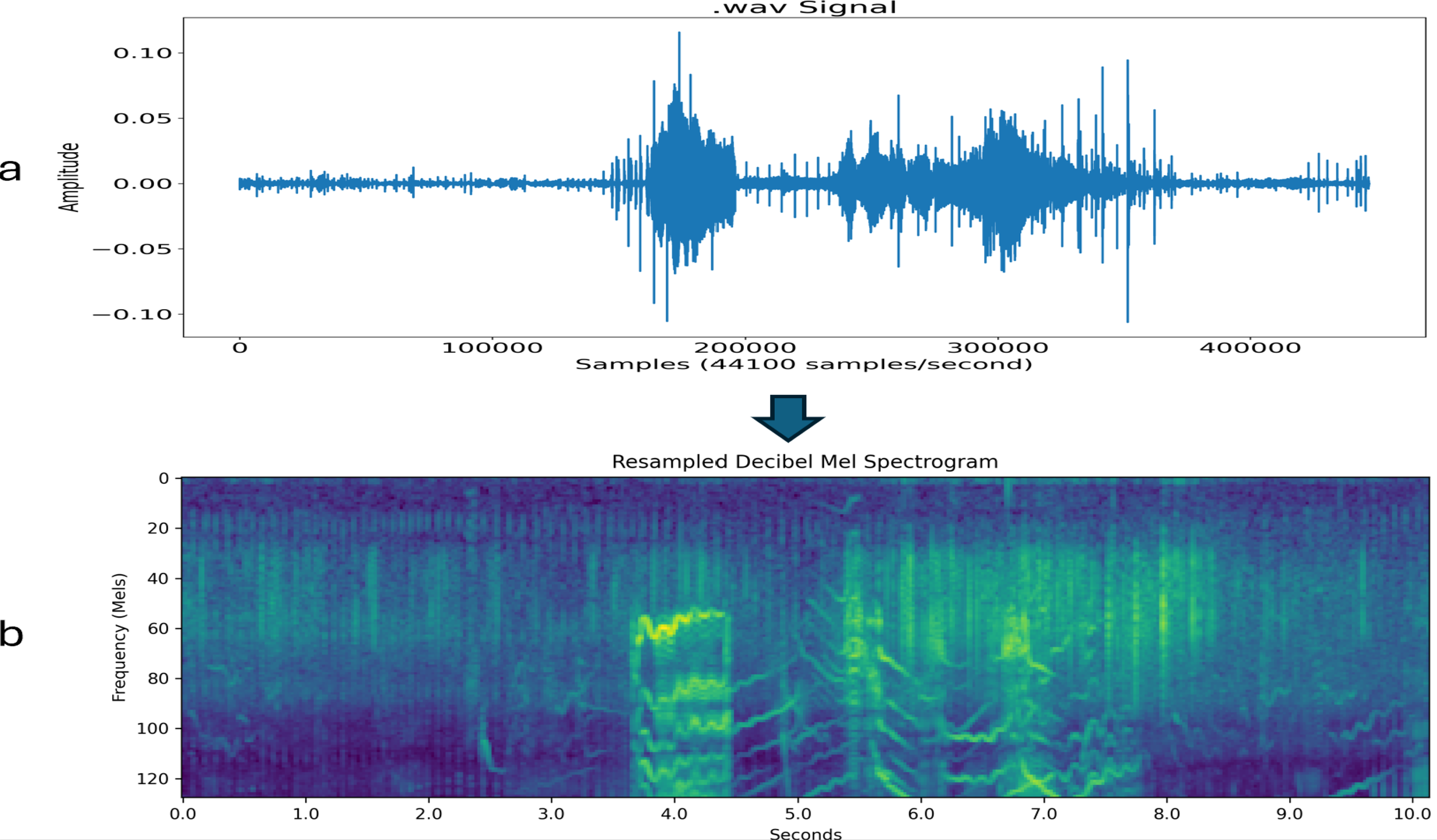
Key steps of the programmatic part of my sound processing pipeline illustrated on a 10-second orca sound segment. (a) Raw recorded sound signal (that is,.wav format) that shows pressure (amplitude) at the sampling points. (b) Resampled Decibel Mel spectrogram. (The padding is not shown in these figures. It would show as a narrow, dark border around the entire image. The normalization of the decibel Mel spectrogram to make a decibel Mel spectrogram image is also not shown. The decibel Mel spectrogram image looks the same as the decibel Mel spectrogram.).
Next, the segments were resampled to a sampling rate of 21,900 samples per second using a Python (version 3.9.13) program which I wrote using the Librosa and NumPy libraries (McFee et al., 2022; Harris et al. 2020). The sampling rate of 21,900 samples per second was chosen since this is the smallest sampling rate I have seen for orca vocalization recordings and I wanted the system to be applicable to the majority of available data. The segment spectograms were also cut from the bottom and the top to have a minimum frequency of 100 Hz and a maximum frequency of 9000 Hz in order to remove superfluous noise. The minimum frequency was set at 100 Hz since this was the minimum frequency observed by (Wellard et al., 2020a) for the orca vocalizations. I did not carefully tune the top cutoff, but 9000 Hz led the system to reach a bigger gap between sound classification accuracy and silence classification accuracy (shown in Table 3) than a cutoff of 11350 Hz, suggesting that the lower top cutoff helped the system focus on orca vocalizations rather than session-specific ambient high-frequency sounds. These steps were taken to standardize the images of the spectrograms so that the convolutional neural network could perform the necessary matrix calculations on the image.
Table 3
| Weighted mean accuracy | Weighted mean validation loss |
|---|---|
| 86.1% | 1.4 |
The system’s weighted mean accuracy and weighted mean validation set loss when classifying silence extracts from all recordings.
One silence extract of one to two seconds in length was taken from every recording in (Wellard et al., 2020b) that had silences and yielded segments. The silence extracts were weighted to be proportional to the number of segments coming from the same recording as the silence extract. The silence extracts were classified by the 20 networks from the cross-validation in Section 3.1.
Then, in order for my deep learning system, which is explained in detail in Section 2.2, to effectively analyze the segments, I transformed the waveforms of the segments into decibel Mel spectrogram images that is, decibel spectrogram images that use the Mel frequency scale as opposed to Hz—as follows. I first transformed the waveforms into Mel spectrograms. A spectrogram takes the Fast Fourier Transform at every time block (i.e., time window); in this case, the window size was 2048 samples with a “stride” of 512, that is, the next window overlaps the previous window by 75%. It ends up being a picture with discrete time steps on the x-axis, frequency in Hertz (Hz) on the y-axis, and strength of each particular frequency as the intensity of the (monochrome) color. This enables one to not only study frequencies that are present in the sound but changes in the frequencies across time. Then, to get a Mel spectrogram, I transform the frequency axis nonlinearly so that the spacing between the harmonics is normalized. Then, I transformed the Mel spectrograms to decibel Mel spectrograms by putting the color intensity (i.e., strength of each frequency) on a log scale. As shown in Figure 2b, this transformation makes the patterns dramatically more noticeable. Finally, I normalize the decibel Mel spectrograms to have values between 0 and 255, which creates a normalized decibel Mel spectrogram image. The image does not look any different than the decibel Mel spectrogram. I used a program I wrote in Python to complete this process. I used these images as inputs for my deep learning system.
When the images are loaded into the deep learning system as input, 3 zero pixels of padding are added to each of the four sides of the spectrogram image. Such padding is used to prevent the convolution layers from unduly focusing on the center of the image. The number 3 is the standard amount of padding given that the convolution kernels are of size 7x7.
2.2 Deep learning system and dealing with potentially superfluous behavior labels
The deep learning system, which I coded in Python using the PyTorch and NumPy libraries, leverages a pre-trained ResNet-34 convolutional neural network and a custom loss function. ResNet-34 is a modern convolutional neural network architecture that includes ReLU units and skip connections (He et al., 2016). It has 34 layers which alternate between convolutional layers and pooling layers4. The final output layer is a fully connected layer. The motivation for pretraining is that the network is likely to learn on small datasets better and learn the real task faster if it is pretrained in advance. Note, however, that ResNet-34’s pretraining was on images (ImageNet) not sounds5. I used the pretrained weight file ImageNet1K V1 [res]. ResNet-34 was originally designed for 1,000 outputs, that is, classes of images. Since our data set only has four orca behaviors that the network is trying to predict, I modified the ResNet architecture to be four-headed, that is, to have four outputs.
Additionally, I modified the ResNet architecture further by removing the normalization. Each input sound segment has a different length. The ResNet34 architecture is able to accommodate different-sized inputs. However, the Pytorch dataloaders, which I use to create minibatches for the network, cannot accommodate different-sized data within a single batch. This meant that I had to set the batch size to 1. It is well known that batch normalization layers in Resnet34 do not work well with small batch sizes. Indeed, I tried batch normalization, layer normalization, instance normalization, and no normalization, and no normalization performed best. Thus, I decided to go with no normalization by making the normalization layers simply be the identity mapping.
Capturing fine-temporal-resolution orca behavior data together with sound would be extremely difficult. Wellard et al. (2020a) labeled their sound recordings with all the behaviors observed during the recording period. For this reason, the majority of the sound segments had potentially superfluous labels. This is due to the fact that, while the orcas were doing all of the labeled behaviors during a given recording, they may not have been doing all of those behaviors in each sound segment within the recording, so the segments have potentially superfluous labels. The potentially superfluous labels on the segments create a difficult classification problem since there is no ground truth (except for certain sound segments where the only behavior label was T, Table 2).
I developed the following approach for dealing with the issue of potentially superfluous behavior labels. We assume that only one behavior was present during each sound segment6. This enables us to leverage recent theory of partially labeled learning (PLL). In PLL, each training instance may have multiple labels, but only one of them is correct. For PLL, Feng et al. (2020) proved that the loss function seen in Equation 1 is risk consistent7. They also introduced a classifier-consistent loss function but showed that especially when using deep learning as the classifier, the risk-consistent loss function performs significantly better in practice. They also showed that the risk-consistent loss function outperforms prior techniques for PLL from the literature (Feng and An, 2019; Cour et al., 2011; Zhang and Yu, 2015; Zhang et al., 2017; Hüllermeier and Beringer, 2005). For these reasons, I use it as the custom loss function for the neural network. This custom loss function enables the network to learn from training data with potentially superfluous labels.
Here the index o is used to sum over instances and the index i to sum over labels. The feature vector (decibel Mel spectrogram in my setting) is . The network’s prediction for instance o is . The label set of training instance o is . The values are, of course, not accessible given the data, so we compute them as the softmax’d version of the network’s output but only if the label is actually a candidate label in the label set (as Feng et al. (2020) do). The formal definition of the softmax is shown in Equation 2
and is computed as shown in Equation 3:
Finally, is the cross entropy loss of the softmax’d predictions, as shown in Equation 4.
As is typical in neural network applications, the neural network was trained using backpropagation with the Adam algorithm (Kingma and Ba, 2014). My software changed the learning rate on a schedule. It started with a learning rate of 8 · 10−5. It decreased the learning rate by a factor of 10 every 15 training epochs.
2.3 Experimental methodology
I evaluated the machine learning model over 20 cross-validation repetitions. Each network in the cross-validation was trained for 30 epochs. I split the sound segments (i.e., instances) into a validation set and a training set so that 20% of the data went to the validation set and 80% went to the training set—in a way that the numbers of segments with each of the behavior label combinations were 80–20 proportionate across the training and validation set. The validation set was not used for training and was used to evaluate the model’s classification accuracy and validation set loss at each epoch. For each repetition in the cross-validation, the validation and training sets needed different instances. For this reason, I shuffled the segments before assigning them to the validation or training set. I used mini-batches of size 1 training instance (sound segment) for training and testing.
One potential concern one might have is that the system could be learning to classify different groups of orcas (with their group-specific vocal repertoire and behaviors) instead of learning to predict behavior based on vocalizations. To provide evidence against that, I also conducted an experiment where I trained the network on the data from the other encounters and tested the system on the data from the remaining one encounter. This experiment also mimics a real-world scenario where the deep learning system would be trained on previous encounters but used on novel encounters. I performed this experiment six ways, using the data from the six encounters on 01/11/2013, 01/08/2013, 12/26/2012, 12/29/2012, and 01/03/2013 that did not have the labels {T,F,M} or {T,F,S,M}. I did not use the encounters which had the labels {T,F,M} or {T,F,S,M} since, due to the classification being considered correct if one of the behaviors in the behavior label combination is the predicted label, these experiments by random guessing would have a 75% and 100% validation set classification accuracy, respectively. Additionally, I conducted an analysis shown and explained in the Appendix where I used the model’s second-to-last layer activations as points for UMAP (McInnes et al., 2018) dimensionality reduction. This analysis suggested that the model learned to classify behaviors, as desired, as opposed to recording session.
3 Results
3.1 Main experiment
As a performance benchmark and a sanity check, I calculated the accuracy that would be achieved by guessing randomly or by always guessing the same single behavior. I found that guessing uniformly at random would achieve 52.9% accuracy. Always guessing T, the most prevalent behavior (with 372 of the segments having T as a possible label), would achieve 75.3% accuracy, as shown in Table 4.
Table 4
| Guess | Analytically calculated accuracy |
|---|---|
| Uniform random among T, F, S, and M | 52.9% |
| Uniform random among only T, F, and S | 60.7% |
| Uniform random among only T and F | 72.1% |
| Always guess T | 75.3% |
| Always guess F | 68.8% |
| Always guess S | 37.9% |
| Always guess M | 29.8% |
Sanity check: accuracy that would result from various guessing schemes based on data from Table 2.
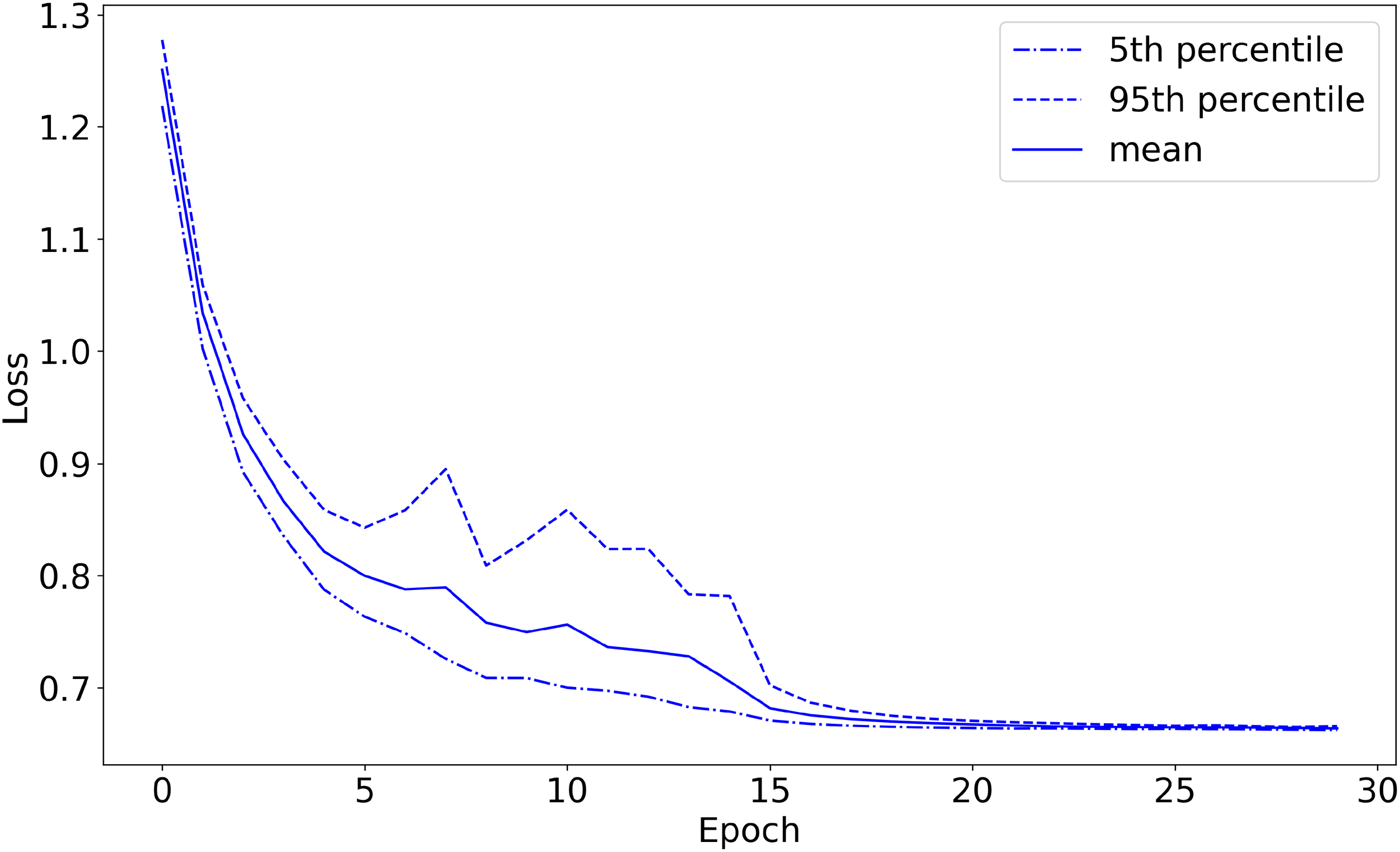
I defined the accuracy on the validation set so that if the network’s highest-predicted-probability behavior was among the (potentially more than one) labels assigned by Wellard et al. for the sound recording from which the sound segment came, the prediction is considered correct. For example, the network could classify a {T,S,F,M} file as either {T}, {F}, {S}, or {M}, but could only classify a {T} file as {T} in order to get the classification correct. The machine learning model achieved 96.1% classification accuracy on the validation set, converged to 1.03 loss on the validation set, and converged to 0.66 loss on the training set, shown in Figures 3–5, respectively. The high accuracy and the loss converging to a low value means that the system was able to learn the task well.
Figure 3
Training set loss as a function of training epochs (with 20-fold cross-validation). The plot starts before the first training epoch has been completed.
Figure 4
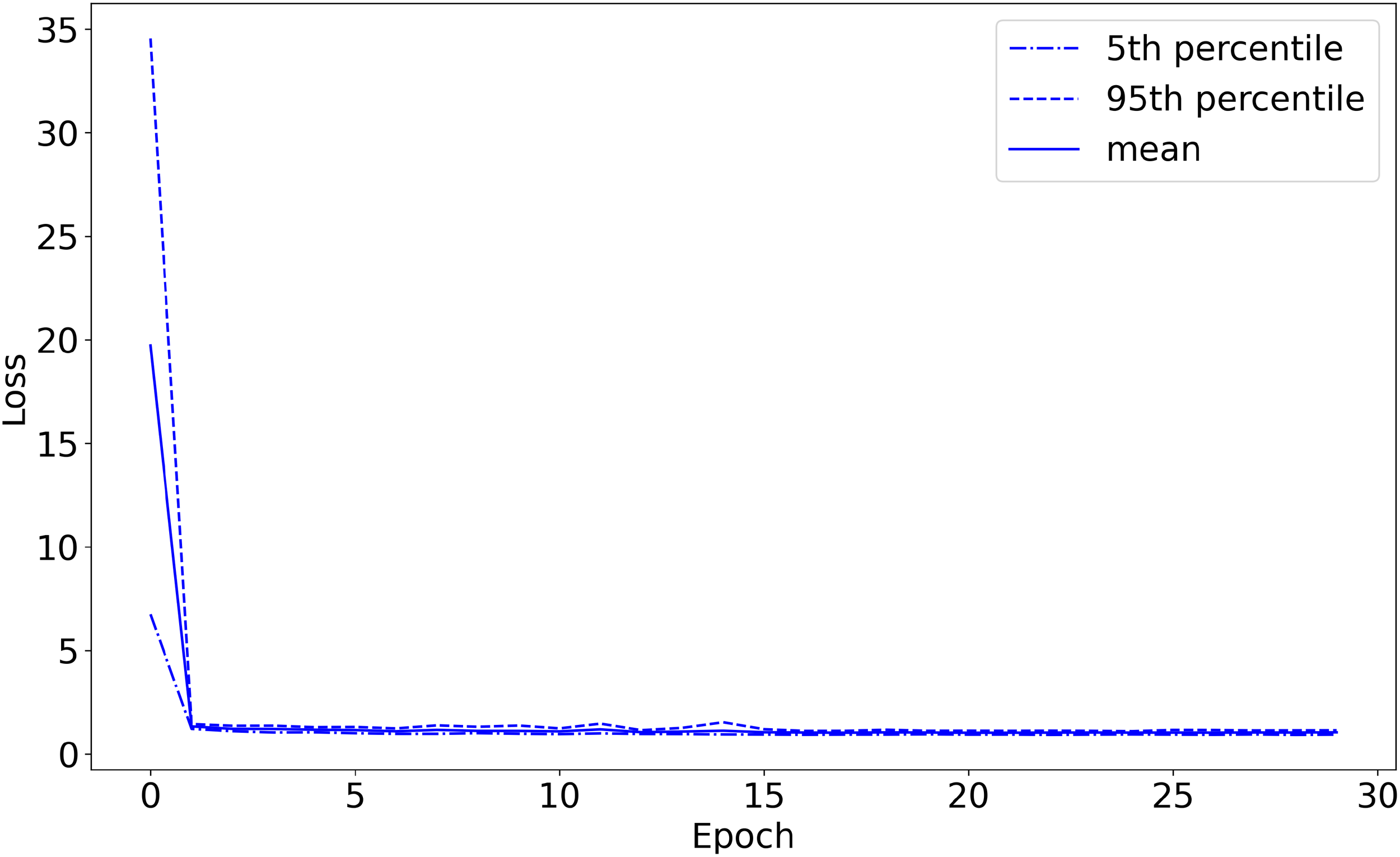
Validation set loss as a function of training epochs (with 20-fold cross-validation). The plot starts before the first training epoch has been completed.
Figure 5
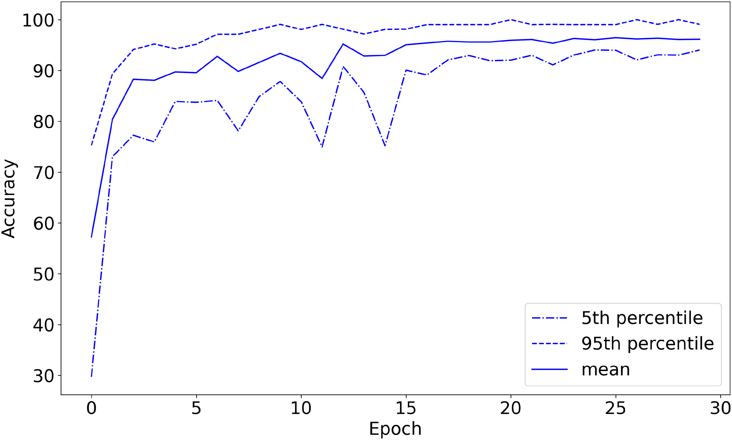
Validation set classification accuracy (%) as a function of training epochs (with 20-fold cross-validation). The plot starts before the first training epoch has been completed.
Given that the system achieved 96.1% accuracy, which is higher than the 75.3% achievable by guessing the most prevalent class, one can see that the orca sound segments had predictive value for behavioral labels. Even at bottom 5% percentile, the model achieved 94.0% accuracy, seen in Figure 5, which is higher than the 75.3% accuracy that the model would achieve if guessing the most prevalent class. Therefore, the model is better than always guessing the most prevalent class with more than 95% statistical significance. These results strongly show that orca sound segments contain indications of behavior.
3.2 Testing on new encounters
As seen in Figures 6 and 7, the system had a validation set classification accuracy ranging from 13.9% to 68.8% (52.6 +/- 19.8) and a loss of 0.64 to 0.78 (0.69 +/- 0.06). The exact values for the mean classification accuracies and training losses for these experiments can also be seen in Table 5.
Figure 6
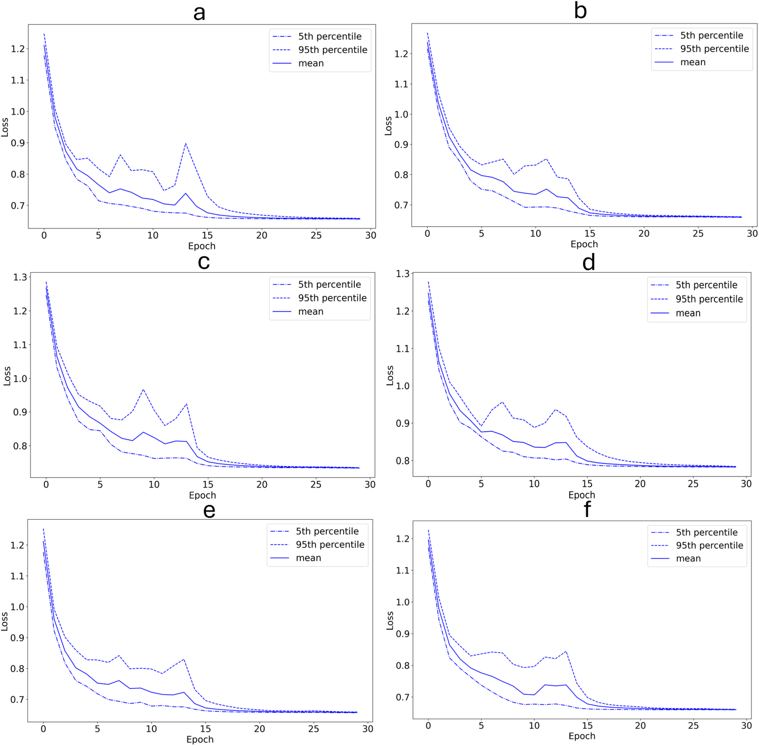
Training set loss as a function of training epochs (with 20-fold cross-validation). (a) The 12/29/2012 encounter with the label combination {F,S} is used as the validation set. (b) The 12/26/2012 encounter with the label combination {F,S} is used as the validation set. (c) The 01/11/2013 encounter with the label combination {T} is used as the validation set. (d) The 01/08/2013 encounter with the label combination {T} is used as the validation set. (e) The 01/08/2013 encounter with the label combination {T,F} is used as the validation set. (f) The 01/03/2013 encounter with the label combination T,S is used as the validation set. The plot starts before the first training epoch has been completed.
Figure 7
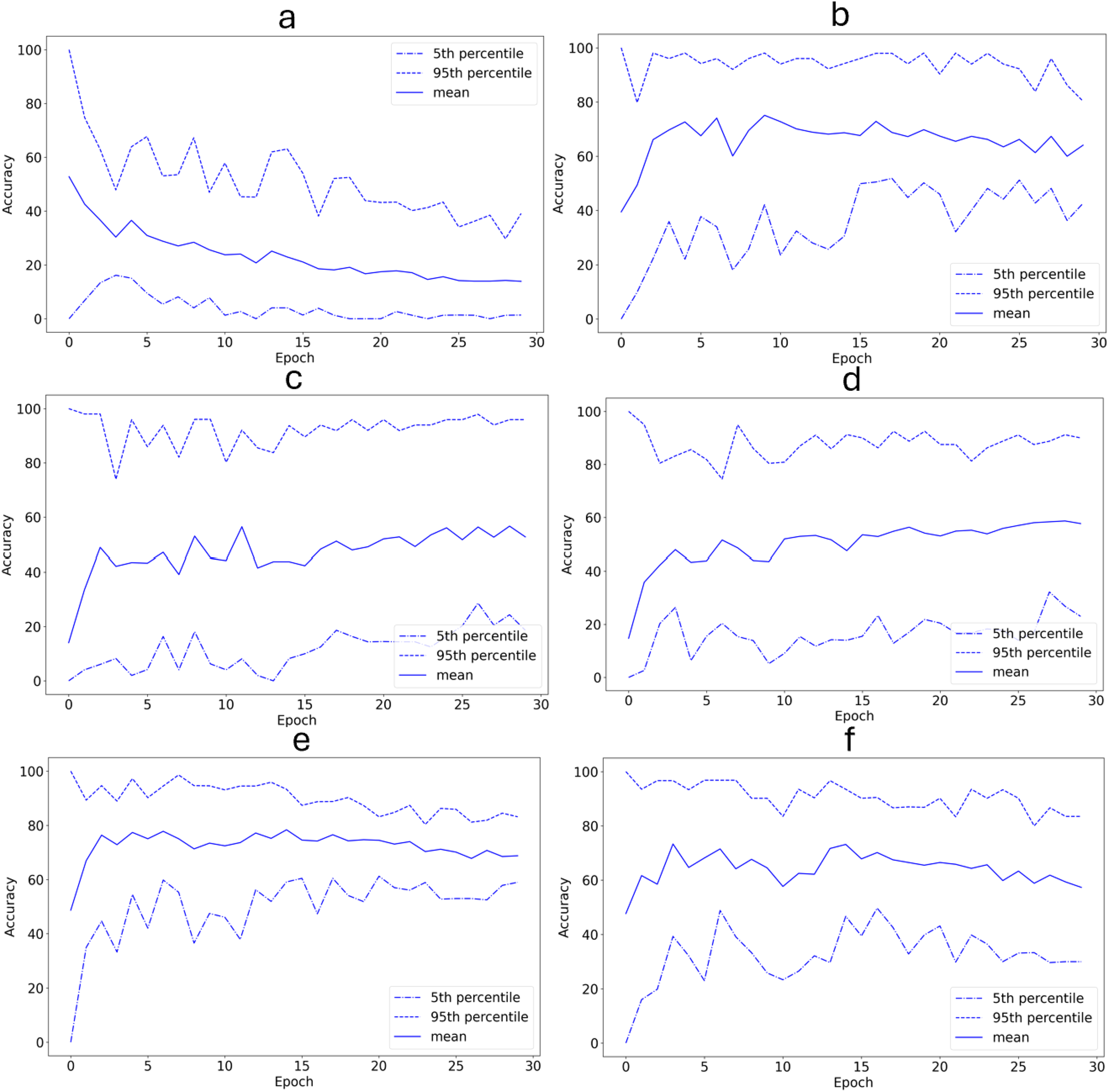
Validation set classification accuracy (%) as a function of training epochs (with 20-fold cross-validation). (a) The 12/29/2012 encounter with the label combination {F,S} is used as the validation set. (b) The 12/26/2012 encounter with the label combination {F,S} is used as the validation set. (c) The 01/11/2013 encounter with the label combination {T} is used as the validation set. (d) The 01/08/2013 encounter with the label combination {T} is used as the validation set. (e) The 01/08/2013 encounter with the label combination {T,F} is used as the validation set. (f) The 01/03/2013 encounter with the label combination T,S is used as the validation set. Epochs are labeled from 0, so the plot starts before the first training epoch has been completed.
Table 5
| Encounter date | Label combination | Mean accuracy on validation set | Mean training set loss |
|---|---|---|---|
| 12/29/2012 | {F,S} | 13.9% | 0.65 |
| 12/26/2012 | {F,S} | 64.1% | 0.64 |
| 01/11/2013 | {T} | 52.7% | 0.73 |
| 01/08/2013 | {T} | 58.7% | 0.78 |
| 01/08/2013 | {T,F} | 68.8% | 0.66 |
| 01/03/2013 | {T,S} | 57.33% | 0.66 |
Date, behavior label, mean validation set classification accuracy, and mean training set loss for each of the six encounters used as a validation set in Section 3.2.
3.3 Examples of what the system predicted
In this section, I show six examples of the system’s predictions for six exogenously chosen sound segments. I show resampled decibel Mel spectrograms of these segments in Figures 8–13, respectively. I show the softmax’d predictions, i.e., the networks predicted probabilities for each behavior class, that the system outputs in Table 6.
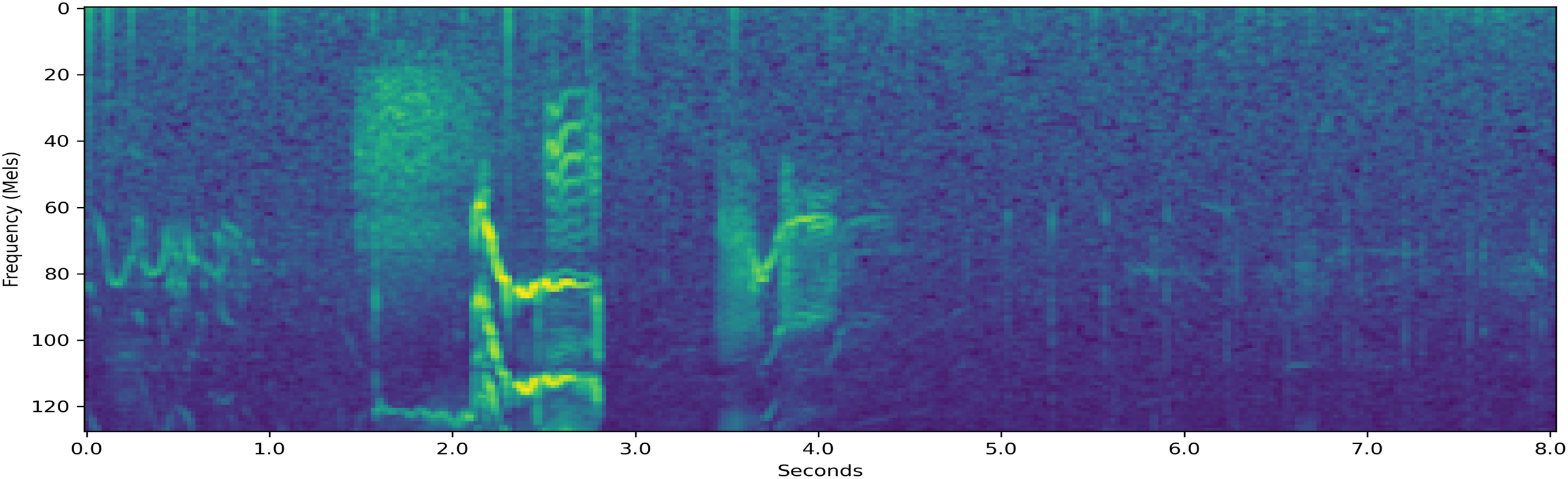
Figure 8
Resampled decibel Mel spectrogram of a 2.6-second-long {T,F,S,M} segment which the system classifies.
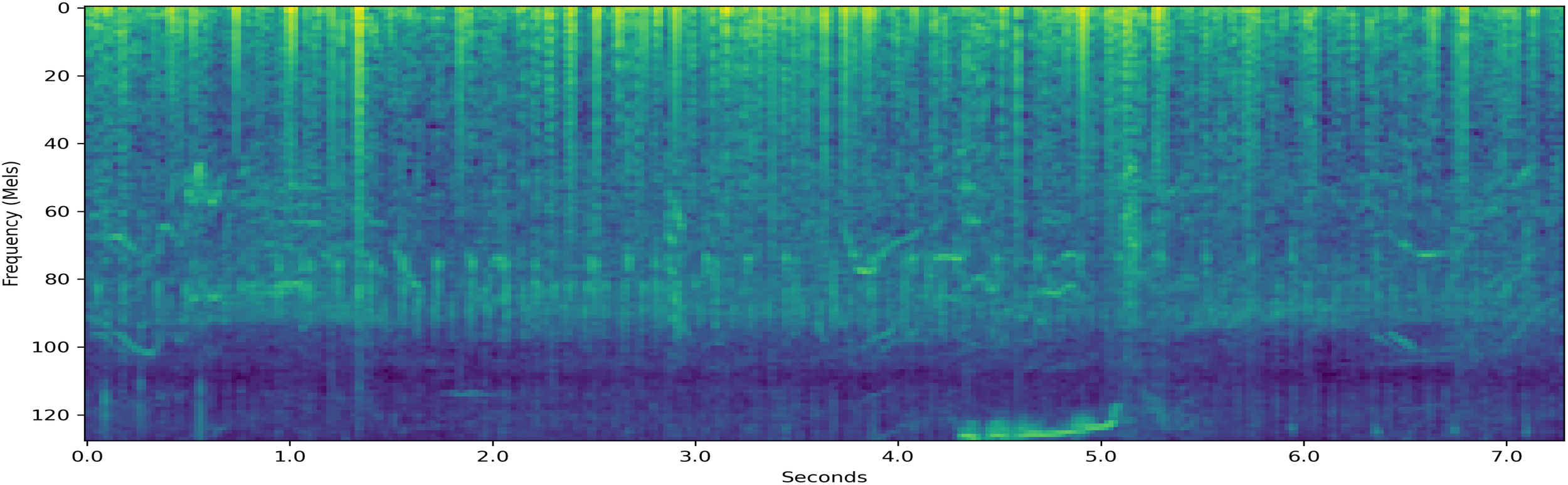
Figure 9
Resampled decibel Mel spectrogram of a 8.0-second-long {T,F} segment which the system classifies.
Figure 10
Resampled decibel Mel spectrogram of a 7.3-second-long {T,F,M} segment which the system classifies.
Figure 11
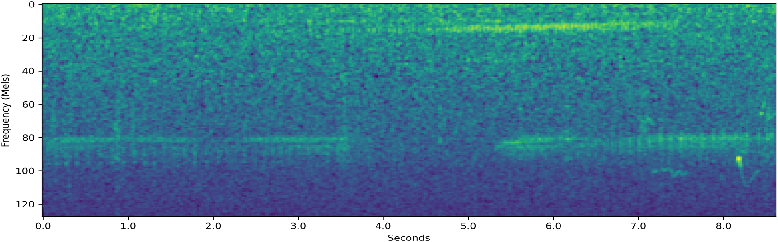
Resampled decibel Mel spectrogram of a 8.6-second-long {T,S} segment which the system classifies.
Figure 12
Resampled decibel Mel spectrogram of a 15.9-second-long {F,S} segment which the system classifies.
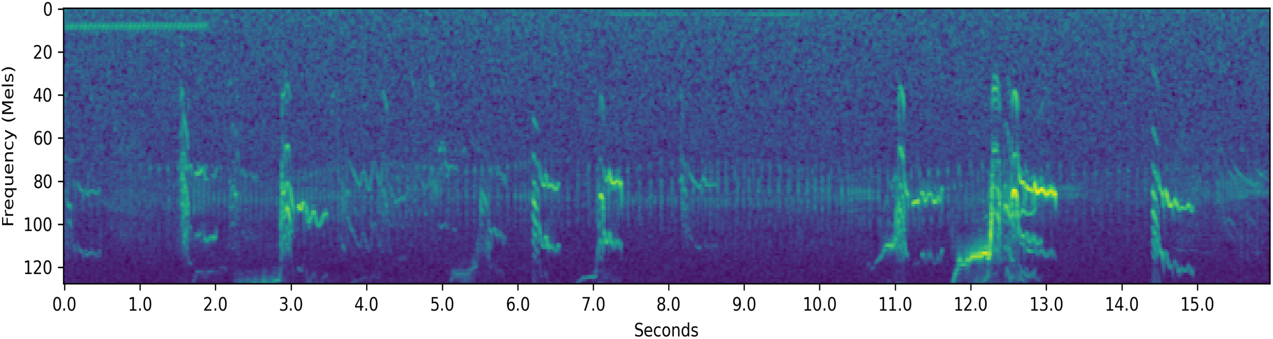
Figure 13
Resampled decibel Mel spectrogram of a 11.5 -second-long {T} segment which the system classifies.
Table 6
| Class | {T,F,S,M} | {T,F} | {T,F,M} | {T,S} | {F,S} | {T} |
|---|---|---|---|---|---|---|
| T | 43.9% | 48.7% | 44.3% | 43.8% | 0.9% | 44.8% |
| F | 32.5% | 36.4% | 33.1% | 32.2% | 14.2% | 31.9% |
| S | 24.1% | 8.9% | 12.5% | 14.6% | 84.1% | 12.6% |
| M | 9.2% | 6.0% | 10.4% | 9.2% | 0.8% | 10.6% |
Figure 8 is a resampled decibel Mel spectrogram of a segment that is spuriously labeled as {T,F,S,M} in the input data, that is, the input data has no information about the correct behavior: having all the labels in the label set means that the input data has no information on that instance. The system classifies this sound as indicating behavior T. This is shown in Table 6. The system assigns probability 43.9% on the behavior being T out of all four behaviors. The network was very sure that the behavior was not M, showing that the system was able to find predictive structures within the segment. It is also possible that certain orca behaviors have structures within the sound segments that are more similar to certain behaviors than to others. In this example, the network was 43.9% sure that the behavior was T and 32.5% sure that the behavior was F. This may suggest that the traveling and socializing have similarities in their vocalization structures.
Figure 9 is a resampled decibel Mel spectrogram of a sound segment that had label set {T,F} in the input data. The system assigns probability 48.7% on the behavior being T, shown in Table 6. The system assigned small probabilities of 8.9% and 6.0% to the behaviors S and M, respectively, which shows that the system was able to detect the two correct labels in this case.
Figure 10 is a resampled decibel Mel spectrogram of a sound segment that had the potentially superfluous label set {T,F,M} in the input data. The system assigns a probability 44.3% on the behavior being T. Although S was the only behavior not included in the set of potential labels, the system assigned a probability of 12.5% to the behavior being S, which is higher than the 10.4% probability the system placed on the behavior being M. In fact, as seen in Table 6, the system assigned the lowest probability to the behavior M for all 6 examples. This may be due to the small amount of segments with the potential label M when compared to the other behaviors.
Figure 11 is a resampled decibel Mel spectrogram of a sound segment that had the label set {T,S}. The system assigned a probability 43.8% on the behavior being F. The system assigned a probability of 14.6% on the behavior being S, which shows that the system was able to differentiate between the two possible labels well. While the socializing behavior was in the set of potential behaviors for this segment, the system predicted that the socializing behavior likely did not occur during this segment. This is a reasonable real-world possibility for this segment, but cannot be fully verified due to the partially labeled nature of the data. The system assigned a probability of 32.2% on the behavior being F, which is rather high considering that F was not one of the correct labels. Additionally, the system is fairly certain that the label was not M, assigning a probability of 9.2% on the behavior being M. It is worth noting that for all the examples where T was a potential label, the system placed the highest probability on the behavior T, followed by F, S, and M in that order. This may be influenced by the high prevalence of segments with the labels T and F in the dataset. However, as seen in Table 4, it is not possible to achieve the system’s 96.1% classification accuracy by simply always guessing T or F.
Figure 12 is a resampled decibel Mel spectrogram of a sound segment that had the label set {F,S}. The system assigned a 84.2% probability on the behavior being S and a 14.2% probability on the behavior being F, revealing that the system could differentiate between the two potentially correct labels for this segment. The system was very certain that the behaviors were not T or M, assigning probabilities of 0.9% and 0.8%, respectively.
Figure 13 is a resampled decibel Mel spectrogram of a sound segment that had the label set {T}. The system assigned a 44.8% probability on the behavior being T. The probability assigned on the behavior F was rather high, with the system assigning the probability 31.9% on the behavior being F.
4 Discussion
Orcinus orca (killer whales) have complex vocalizations that use multiple frequencies simultaneously, vary the frequencies, vary their intensities, and vary their temporal patterns. I used a recent orca sound recording collection that is rare in the sense that it has auxiliary behavior data (Wellard et al., 2020b, a). In particular, it has partially labeled behavior data. By carefully combining and tailoring select recent machine learning techniques, I showed that previously unheard sound segments can be used to predict orca behavior with 96.1% accuracy (although classification accuracy varied considerably among behavioral categories). This revealed the highly predictive properties that orca sound segments have when it comes to classifying behavior. The fact that the sound segments can be used to classify behavior suggests that orcas convey behavior through their vocalizations.
There are many further features of orca vocalizations that may have aided the deep learning system with the task of classifying behavior. These include acoustic markers of directionality, echolocation clicks, the frequency of certain call types in the segments, and features that capture overlapping calls. I will now discuss these, broken out by behavior.
The mammal-eating transient orcas in the Pacific Northwest are known to vocalize primarily after a successful hunt, whereas their fish-eating counterparts, the resident orcas, are known to vocalize more consistently (Deecke et al., 2005). Deeke et al. suggested that the difference in the transient and resident populations’ vocal behavior is due to their feeding habits. According to Barrett-Lennard et al. (1996), fish-eating orcas also echo-locate using sonar trains more frequently than mammal-eating orcas. Additionally, they found that the fish-eating residents were more likely to echo-locate during foraging than any other behavior. Given that the Type C orcas whose vocalizations are analyzed in this paper are primarily fish eaters and echolocation clicks were analyzed as part of the vocalizations, it is quite possible that the echolocation clicks provided a feature that may have contributed to the classification accuracy of foraging. Indeed, segments that had foraging in their behavior label set were classified better than those that did not include foraging, with the exception of the segments from the 12/29/2012 encounter. While echolocation clicks are thought to be a way for orcas to observe their physical location and not socially communicating, they still add to the underwater soundscape and may serve as a form of indirect communication. Regardless, for the purposes of determining orca behavior from vocalization data, the echolocation clicks may be a useful feature for the model.
Ford (1989) found that during socializing, resident orcas were highly vocal and exhibited high frequencies of certain calls, namely whistle, aberrant, and variable calls. It is possible that in my study such higher frequencies of these calls may have contributed to the classification accuracy of socializing. Additionally, socializing implies that many individuals are present so there is a possibility that overlapping calls from many orcas provided a classifiable feature in socializing segments.
Lastly, orcas are known to exhibit significantly less vocal activity during milling than the other three behavioral states (Ford, 1989). The reduced frequency of calls and vocal activity, in general, may have contributed to the classification accuracy of milling segments. My methodology of removing quiet periods longer than two seconds between vocalizations would have mitigated this. However, it is possible that this effect is still present to some extent because milling recordings may have had more quiet periods of length less than two seconds.
The system had some difficulty when classifying segments from novel encounters. This can be seen by the low classification accuracies in Table 5. The classification accuracy for the 12/29/2012 encounter with behavior label F,S was particularly low with a mean accuracy of 13.9%. This may be due to the fact that the segments from the 12/29/2012 encounter contain significantly more echolocation clicks than most of the segments from the other encounters. Since the dataset used is small with only 494 segments, removing the data from an encounter removes a significant amount of potential training data. This may have contributed to the low accuracies. However, as seen by the low training loss values in Table 5, the system was able to learn on the training set. This may be an indication of overfitting on the training set.
A major limit to my study, the lack of ground truth, comes from our use of partially labeled data. The lack of ground truth means that I am not able to determine with greater precision the accuracy of the network. As an extreme example, for a {T,F,S,M} segment, any behavior classification is considered correct. Additionally, the data being only partially labeled made it impossible to analyze the classification accuracy for each behavior class separately. A way to remedy this issue would be to train the network on fully labeled data.
Another limitation of this study is potential differences in the segments based on group identity rather than behavior. The data set did not include associated group identity information, so it was not possible to determine explicitly that group identity was independent of the behavior labels of the segments. Subject to the available data, I conducted the experiments in Section 3.2 where I used each individual encounter as the validation set in turn. The classification accuracies for these experiments were low, although four out of the six experiments had mean accuracies that were better than random guessing. It is possible that the low classification accuracies are a result of removing significant amounts of data from the training set. If this is true, the classification accuracies in these experiments may increase if the system is trained on more data.
It is also possible that the system learned to classify the recording session as opposed to the behaviors. However, as shown in Table 3, I used the system to classify silence extracts from each of (Wellard et al., 2020a)’s recordings. These silence extracts should contain the session information. The system performed significantly worse on the silence extracts compared to the sound segments, which suggests that the system did not just learn the session instead of the behaviors. Additionally, as shown in the Appendix, the system’s activations at the second-to-last layer differentiated between behavior label combinations, suggesting that the system learned behavior instead of recording session.
To my knowledge, this paper is the first to use partially labeled learning to study animal vocalizations and the first to use machine learning to analyze orca sound segments beyond individual calls.
As shown by Williams et al. (2024), pretraining on bioacoustics data can help machine learning systems achieve better performance on bioacoustics tasks. While this was not implemented in this study, incorporating such pretraining could be an avenue for future research.
This work and system could help marine biologists study orca behavior with greater capacity. Currently, observing orca behavior is quite difficult since orcas live under water and their behaviors may not be obvious to an above-water observer. The system would be helpful for marine biologists because it would allow marine biologists to record orca vocalizations and identify orca behaviors with greater ease and efficiency. Naturally, users would need to understand that the predictions are not perfect and vary across predicted behaviors. Further prediction accuracy could be achieved with fully labeled training data.
The system could also aid further research into whale language. For example, one could use the segments that the algorithm classified as being associated with a certain behavior and compare the structure of segments where the orcas are exhibiting different behaviors to study the differentiating features. This would give researchers insight into the potential grammar structure of orca language. The algorithm may also contribute to the development of more data sets with behavior labels, which would allow researchers working on orca language to have more data with which to work. For one, this could allow for greater ease and creativity when studying orca language with machine learning.
5 Appendix
To further address the concern of the model learning recording session instead of behavior, I completed an additional analysis where I took the activations of the second-to-last layer of the network and used UMAP (McInnes et al., 2018) to reduce the dimensions of these high-dimensional points to two dimensions 8. I then plotted these dimensionality-reduced points and colored the points by recording session. This plot can be seen in Figure 14. I also plotted the dimensionality-reduced points using the network’s prediction for each behavior as the opacity of the points. I also marked the behavior label combination to which the majority of the points in each cluster in Figure 14 corresponded. These plots can be seen in Figures 15a–d.
Figure 14
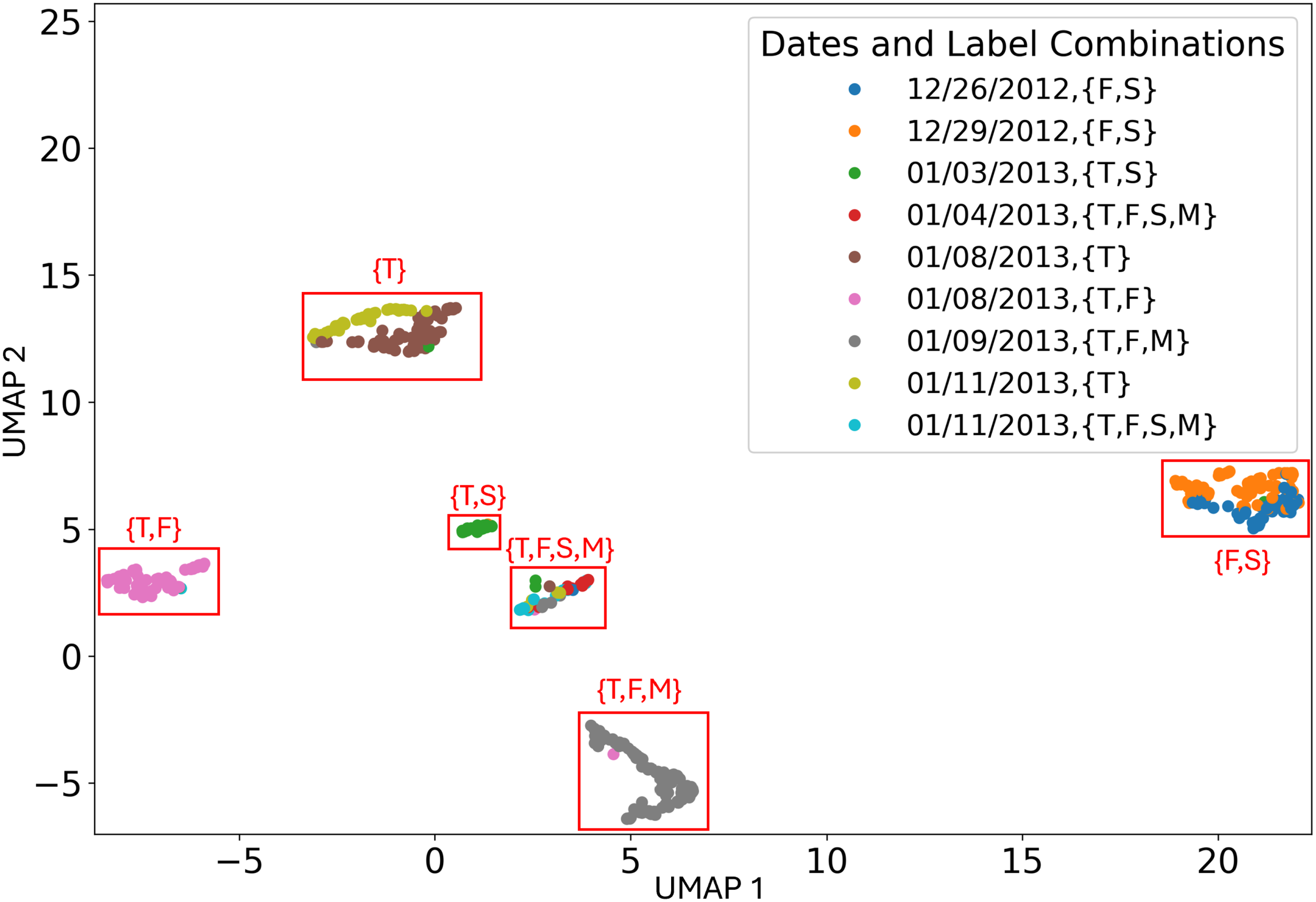
Scatter plot of the UMAP dimensionality-reduced activations from the second-to-last layer of the model. The behavior label combination corresponding to the majority of the points in each cluster is also shown.
Figure 15

Scatter plot of the UMAP dimensionality-reduced activations from the second-to-last layer of the model using the network’s prediction probabilities for each behavior as the opacity for each point. (a) The model’s prediction probabilities for behavior {T} are used as the opacity for each point. (b) The model’s prediction probabilities for behavior {F} are used as the opacity for each point. (c) The model’s prediction probabilities for behavior {S} are used as the opacity for each point. (d) The model’s prediction probabilities for behavior {M} are used as the opacity for each point.
As seen in Figure 14, the points formed six clusters, each of which corresponded to one of the six behavior label combinations. In each cluster, the overwhelming majority of the points had the corresponding label combination. The cluster corresponding to the {T,F,S,M} behavior label combination contained more points with other behavior label combinations than the other clusters. This could be because the network may have mapped points where the network was more uncertain of the behavior label to that cluster. Additionally, three of the clusters contained points from multiple recording sessions. The three clusters that did not contain many points from multiple recording sessions corresponded to behavior label combinations that were only observed during a single recording session. Thus, the points appear to be clustered based on behavior label combination. This suggests that the network learned behavior, as desired, as opposed to the recording session. The percentage of data points in each cluster with the corresponding behavior label combinations can be seen in Table 7.
Table 7
| Cluster Behavior Label Combination | Percentage of Points in Cluster with Given Label Combination |
|---|---|
| {F,S} | 99.2% |
| {T,S} | 96.0% |
| {T,F,S,M} | 73.5% |
| {T} | 97.5% |
| {TF} | 95.8% |
| {T,F,M} | 99.1% |
The percentage of points in each UMAP cluster with the behavior combination of the majority of points in that cluster.
As seen in Figures 15a–d, the network placed high probabilities on only correct behaviors for five out of the 6 behavior label combinations. This further suggests that the network learned behavior instead of the recording session. The one cluster where high probabilities were placed on an incorrect behavior was the {F,S} cluster, where a relatively high probability was placed on the incorrect behavior {T} for many of the points in this cluster.
Statements
Data availability statement
The original contributions presented in the study are included in the article/supplementary material, further inquiries can be directed to the corresponding author.
Ethics statement
Ethical review and approval was not required for the study on animals in accordance with the local legislation and institutional requirements.
Author contributions
SS: Conceptualization, Formal analysis, Data curation, Investigation, Methodology, Software, Validation, Visualization, Writing – original draft, Writing – review & editing.
Funding
The author(s) declare that no financial support was received for the research and/or publication of this article.
Acknowledgments
I would like to thank Professor Tuomas Sandholm for advising my research. I would like to thank Dr. Christina Fong-Sandholm for aiding in the research process. I would also like to thank Dr. Cindy Elliser and two reviewers for helpful comments.
Conflict of interest
The author declares that the research was conducted in the absence of any commercial or financial relationships that could be construed as a potential conflict of interest.
Publisher’s note
All claims expressed in this article are solely those of the authors and do not necessarily represent those of their affiliated organizations, or those of the publisher, the editors and the reviewers. Any product that may be evaluated in this article, or claim that may be made by its manufacturer, is not guaranteed or endorsed by the publisher.
Footnotes
1.^The ResNet-18 neural network is a type of convolutional neural network, similar to the ResNet-34 convolutional neural network used in this paper, but with just 18 layers [He et al., 2016].
2.^For January 8th and January 11th, where the orcas were recorded at two separate locations on the same day and a different set of behaviors was observed during each recording, I used the individual calls [documented by Wellard et al. (2020a)] observed during each encounter to identify which recordings were associated with which encounter. To do this, I performed a preliminary analysis using Audacity (version 3.4.2) to look at the spectrogram of the sound and identify the presence of certain call types which only occurred during a given behavior label combination. If a recording contained a call type that was only present during one of the two possible encounters, I was able to determine that that recording originated from the encounter where that specific call type was observed. This turned out to always be the case.
3.^No steps were taken to improve audibility. I generated the spectrograms in Audacity using the ”Frequencies” algorithm, a Hann window, window size of 2048, zero padding factor of 1, and the Mel frequency scale.
4.^A ReLU unit is a neural network unit (that is, an artificial neuron) where the output activation is zero if the weighted sum of inputs is negative, and equal to the weighted sum of inputs otherwise. Skip connections are connections that skip at least one layer in the network. Convolution layers apply kernels, i.e., filters, to the image matrix. These kernels transform the image matrix for further processing. Pooling layers reduce the image size to make the image faster for the network to process.
5.^The ImageNet dataset is a preexisting dataset consisting of millions of images of thousands of types of object.
6.^It is conceivable that this assumption may not be fully accurate for some sound segments in the orca context, but as I will show, I get high classification accuracy with it. Also, it is conceivable that multiple orcas could be producing overlapping or back-to-back vocalizations in a given segment and/or that different orcas in a pod could be exhibiting different behaviors during a segment. However, these are not a problem for the model.
7.^Risk consistency means that the empirical loss approaches the minimum possible loss as the amount of training data approaches infinity.
8.^I used a random seed of 37 for this UMAP analysis.
References
1
Allen A. N. Harvey M. Harrell L. Jansen A. Merkens K. Wall C. et al . (2021). A convolutional neural network for automated detection of humpback whale song in a diverse, long-term passive acoustic dataset. Front. Mar. Sci.8, 607321. doi: 10.3389/fmars.2021.607321
2
Andreas J. Beguš G. Bronstein M. M. Diamant R. Delaney D. Gero S. et al . (2022). Toward understanding the communication in sperm whales. iScience25, 104393. doi: 10.1016/j.isci.2022.104393
3
Barrett-Lennard L. G. Ford J. K. B. Heise K. A. (1996). The mixed blessing of echolocation: differences in sonar use by fish-eating and mammal-eating killer whales. Anim. Behav.51, 553–565. doi: 10.1006/anbe.1996.0059
4
Bergler C. Schmitt M. Cheng R. X. Maier A. Barth V. Nöth E. (2019b). “Deep learning for orca call type identification – a fully unsupervised approach,” in Proceedings of the Annual Conference of the International Speech Communication Association (INTERSPEECH). Eds. KubinG.HainT.SchullerB.ZarkaD. E.HodlP. (Gratz, Austria: International Speech Communication Association), 3357–3361.
5
Bergler C. Schmitt M. Cheng R. X. Schröter H. Maier A. Barth V. et al . (2019c). “Deep representation learning for orca call type classification,” in International Conference Text, Speech, and Dialogue (TSD), vol. 11697 . Ed. EkšteinK. (Cham, Switzerland: Springer Verlag), 274–286.
6
Bergler C. Schröter H. Cheng R. X. Barth V. Weber M. Nöth E. et al . (2019a). ORCA-SPOT: An automatic killer whale sound detection toolkit using deep learning. Sci. Rep.9, 10997. doi: 10.1038/s41598-019-47335-w
7
Bermant P. Bronstein M. Wood R. Gero S. Gruber D. (2019). Deep machine learning techniques for the detection and classification of sperm whale bioacoustics. Sci. Rep.9, 1–10. doi: 10.1038/s41598-019-48909-4
8
Best P. Marxer R. Paris S. Glotin H. (2022). Temporal evolution of the mediterranean fin whale song. Sci. Rep.12. doi: 10.1038/s41598-022-15379-0
9
Cour T. Sapp B. Taskar B. (2011). Learning from partial labels. J. Mach. Learn. Res.12, 1501–1536.
10
Deecke V. B. Ford J. K. B. Slater P. J. B. (2005). The vocal behaviour of mammal-eating killer whales: communicating with costly calls. Anim. Behav.69, 395–405. doi: 10.1016/j.anbehav.2004.04.014
11
Deecke V. B. Ford J. K. B. Spong P. (1999). Quantifying complex patterns of bioacoustic variation: Use of a neural network to compare killer whale (orcinus orca) dialects. J. Acoust. Soc. America105, 2499–2507. doi: 10.1121/1.426853
12
Deecke V. B. Ford J. K. B. Spong P. (2000). Dialect change in resident killer whales: implications for vocal learning and cultural transmission. Anim. Behav.60, 629–638. doi: 10.1006/anbe.2000.1454
13
Feng L. An B. (2019). “Partial label learning with self-guided retraining,” in Proceedings of the AAAI Conference on Artificial Intelligence (AAAI) (Washington DC, USA: AAAI Press), Vol. 33. 3542–3549.
14
Feng L. Lv J. Han B. Xu M. Niu G. Geng X. et al . (2020). “Provably consistent partial-label learning,” in Conference on Neural Information Processing Systems (NeurIPS) (NY, USA: Curran Associates Inc.).
15
Filatova O. A. (2020). Independent acoustic variation of the higher- and lower-frequency components of biphonic calls can facilitate call recognition and social affiliation in killer whales. PloS One15, 1–15. doi: 10.1371/journal.pone.0236749
16
Filatova O. A. Deecke V. B. Ford J. K. B. Matkin C. O. Barrett-Lennard L. G. Guzeev M. A. et al . (2012). Call diversity in the north pacific killer whale populations: implications for dialect evolution and population history. Anim. Behav.83, 595–603. doi: 10.1016/j.anbehav.2011.12.013
17
Ford J. K. B. (1984). Call traditions and dialects of killer whales (Orcinus orca) in British Columbia. Vancouver, British Columbia: University of British Columbia.
18
Ford J. K. B. (1989). Acoustic behaviour of resident killer whales (orcinus orca) off Vancouver Island, British Columbia. Can. J. Zool.67, 727–745. doi: 10.1139/z89-105
19
Ford J. K. B. (1991). Vocal traditions among resident killer whales (orcinus orca) in coastal waters of British Columbia. Can. J. Zool.69, 1454–1483. doi: 10.1139/z91-206
20
Ford J. K. B. Ellis G. M. Balcomb K. C. (2011). Killer Whales: The Natural History and Genealogy of Orcinus Orca in British Columbia and Washington (Vancouver, British Columbia: UBC Press).
21
Gillespie D. Mellinger D. K. Gordon J. McLaren D. Redmond P. McHugh R. et al . (2009). PAMGUARD: Semiautomated, open source software for real-time acoustic detection and localization of cetaceans. J. Acoust. Soc. America125, 2547–2547. doi: 10.1121/1.4808713
22
Harris C. R. Jarrod Millman K. van der Walt S. J. Gommers R. Virtanen P. Cournapeau D. et al . (2020). Array programming with numPy. Nature585, 357–362. doi: 10.1038/s41586-020-2649-2
23
He K. Zhang X. Ren S. Sun J. (2016). “Deep residual learning for image recognition,” in Proceedings of the IEEE Conference on Computer Vision and Pattern Recognition (CVPR) (NY, USA: IEEE). 770–778.
24
Hüllermeier E. Beringer J. (2005). Learning from ambiguously labeled examples. Intel. Data Anal.10, 419–439. doi: 10.1007/11552253_16
25
Jiang J. Bu L. Wang X. Li C. Sun Z. Yan H. et al . (2018). Clicks classification of sperm whale and long-finned pilot whale based on continuous wavelet transform and artificial neural network. Appl. Acoust.141, 26–34. doi: 10.1016/j.apacoust.2018.06.014
26
Kingma D. P. Ba J. (2014). Adam: A method for stochastic optimization. arXiv. doi: 10.48550/arXiv.1412.6980
27
Leu A. A. Hildebrand J. A. Rice A. Baumann-Pickering S. Frasier K. E. (2022). Echolocation click discrimination for three killer whale ecotypes in the Northeastern Pacific. J. Acoust. Soc. America151, 3197–3206. doi: 10.1121/10.0010450
28
McFee B. Metsai A. McVicar M. Balke S. Thomé C. Raffe C. et al . (2022). librosa/librosa. doi: 10.5281/zenodo.6759664
29
McInnes L. Healy J. Saul N. Grossberger L. (2018). Umap: Uniform manifold approximation and projection. J. Open Source Softw.3, 861. doi: 10.21105/joss.00861
30
Miller B. S. Madhusudhana S. Aulich M. G. Kelly N. (2022). Deep learning algorithm outperforms experienced human observer at detection of blue whale d-calls: a double-observer analysis. Remote Sens. Ecol. Conserv. 9, 104–116. doi: 10.1002/rse2.297
31
Miller P. J. Bain D. E. (2000). Within-pod variation in the sound production of a pod of killer whales, orcinus orca. Anim. Behav.60, 617–628. doi: 10.1006/anbe.2000.1503
32
Murray S. O. Mercado E. Roitblat H. L. (1998). The neural network classification of false killer whale (Pseudorca crassidens) vocalizations. J. Acoust. Soc. America104, 3626–3633. doi: 10.1121/1.423945
33
Pitman R. Ensor P. (2003). Three forms of killer whales (orcinus orca) in Antarctica. J. Cetacean Res. Manage5, 131–139. doi: 10.47536/jcrm.v5i2.813
34
Poupard M. Symonds H. Spong P. Glotin H. (2021). Intra-group orca call rate modulation estimation using compact four hydrophones array. Front. Mar. Sci.8. doi: 10.3389/fmars.2021.681036
35
resnet34 ResNet34 Weights. Available online at: https://docs.pytorch.org/vision/main/models/generated/torchvision.models.resnet34.htmltorchvision.models (Accessed May 17, 2025).
36
Schall E. Van Opzeeland I. (2017). Calls produced by ecotype c killer whales (orcinus orca), off the eckstrom¨ iceshelf, Antarctica. Aquat. Mamm.43, 117–126. doi: 10.1578/AM.43.2.2017.117
37
Schevill W. E. Watkins W. A. (1966). Sound structure and directionality in orcinus (killer whale). Zool.: Sci. contrib. New York Zool. Soc.51, 71–76. doi: 10.5962/p.203283
38
Schröter H. Nöth E. Maier A. Cheng R. Barth V. Bergler C. (2019). “Segmentation, classification, and visualization of orca calls using deep learning,” in IEEE International Conference on Acoustics, Speech and Signal Processing (ICASSP) (NY, USA: IEEE). 8231–8235.
39
Selbmann A. Deecke V. B. Filatova O. Fedutin I. Miller P. J. Simon M. et al . (2023). Call type repertoire of killer whales (orcinus orca) in Iceland and its variation across regions. Mar. Mamm. Sci.39, 1136–1160. doi: 10.1111/mms.13039
40
Shiu Y. Palmer K. J. Roch M. A. Fleishman E. Liu X. Nosal E.-M. et al . (2020). Deep neural networks for automated detection of marine mammal species. Sci. Rep.10, 607. doi: 10.1038/s41598-020-57549-y
41
Simon M. Ugarte F. Wahlberg M. Miller L. A. (2006). Icelandic killer whales orcinus orca use a pulsed call suitable for manipulating the schooling behavior of herring clupea harengus. Bioacoustics16, 57–74. doi: 10.1080/09524622.2006.9753564
42
Weiß B. M. Ladich F. Spong P. Symonds H. (2006). Vocal behavior of resident killer whale matrilines with newborn calves: The role of family signatures. J. Acoust. Soc. America119, 627–635. doi: 10.1121/1.2130934
43
Weiß B. M. Symonds H. Spong P. Ladich F. (2007). Intra- and intergroup vocal behavior in resident killer whales, orcinus orca. J. Acoust. Soc. America122, 3710–3716. doi: 10.1121/1.2799907
44
Wellard R. Pitman R. L. Durban J. Erbe C. (2020a). Cold call: the acoustic repertoire of Ross Sea killer whales (Orcinus orca, type c) in McMurdo Sound, Antarctica. R. Soc. Open Sci.7, 191228. doi: 10.1098/rsos.191228
45
Wellard R. Pitman R. L. Durban J. Erbe C. (2020b). Cold call: the acoustic repertoire of Ross Sea killer whales (Orcinus orca, type c) in McMurdo Sound, Antarctica. Dryad Data Reposit. 7. doi: 10.5061/dryad.37pvmcvfr
46
Williams B. Merrienboer B. v. Dumoulin V. Hamer J. Triantafillou E. Fleishman A. B. et al . (2024). Leveraging tropical reef, bird and unrelated sounds for superior transfer learning in marine bioacoustics. arXiv. doi: 10.48550/arXiv.2404.16436
47
Yurk H. Barrett-Lennard L. G. Ford J. K. B. Matkin C. O. (2002). Cultural transmission within maternal lineages: vocal clans in resident killer whales in southern Alaska. Anim. Behav.63, 1103–1119. doi: 10.1006/anbe.2002.3012
48
Zhang M.-L. Yu F. (2015). “Solving the partial label learning problem: An instance-based approach,” in International Conference on Artificial Intelligence (IJCAI) (Washington DC, USA: AAAI Press). 4048–4054.
49
Zhang M. L. Yu F. Tang C.-Z. (2017). Disambiguation-free partial label learning. IEEE Trans. Knowl. Data Eng.29, 2155–2167. doi: 10.1109/TKDE.69
50
Zhong M. Castellote M. Dodhia R. Ferres J. L. Keogh M. Brewer A. (2020). Beluga whale acoustic signal classification using deep learning neural network models. J. Acoust. Soc. America147. doi: 10.1121/10.0000921
Summary
Keywords
orca, vocalization, calls, behavior prediction, machine learning, partially labeled learning, language, semantics
Citation
Sandholm S (2025) Machine learning to predict killer whale (Orcinus orca) behaviors using partially labeled vocalization data. Front. Mar. Sci. 12:1232022. doi: 10.3389/fmars.2025.1232022
Received
31 May 2023
Accepted
20 May 2025
Published
13 June 2025
Volume
12 - 2025
Edited by
Clea Parcerisas, Flanders Marine Institute, Belgium
Reviewed by
Brigitte Schlögl, Leipzig University, Germany
Maxence Ferrari, UPR7051 Laboratoire de mécanique et d’acoustique (LMA), France
Updates
Copyright
© 2025 Sandholm.
This is an open-access article distributed under the terms of the Creative Commons Attribution License (CC BY). The use, distribution or reproduction in other forums is permitted, provided the original author(s) and the copyright owner(s) are credited and that the original publication in this journal is cited, in accordance with accepted academic practice. No use, distribution or reproduction is permitted which does not comply with these terms.
*Correspondence: Sophia Sandholm, ssandhol@andrew.cmu.edu
Disclaimer
All claims expressed in this article are solely those of the authors and do not necessarily represent those of their affiliated organizations, or those of the publisher, the editors and the reviewers. Any product that may be evaluated in this article or claim that may be made by its manufacturer is not guaranteed or endorsed by the publisher.