Abstract
The study focused on analyzing shoreline changes along the western beaches of Mersin Province, located on Turkey’s Mediterranean coast. Landsat satellite imagery from 1985 to 2022 was used to detect long-term coastal alterations. The Google Earth Engine (GEE) platform facilitated data acquisition, classification, and edge detection. A Support Vector Machine (SVM) classification algorithm was applied to distinguish land from water. To enhance classification accuracy, additional indices—Normalized Difference Water Index (NDWI), Modified NDWI (MNDWI), and Normalized Difference Moisture Index (NDMI)—were incorporated alongside Landsat spectral bands. The Canny edge detection algorithm was employed to delineate shorelines from the classified images. Resulting shoreline positions were analyzed using the DSAS, an open-source ArcGIS extension, to quantify erosion and accretion. Key shoreline change metrics— Net Shoreline Movement (NSM), Shoreline Change Envelope (SCE), End Point Rate (EPR), and Linear Regression Rate (LRR) —were derived from DSAS outputs. Over the 38-year study period, maximum shoreline advancement reached 588.59 meters, while maximum retreat was −130.63 meters. The highest erosion rates were −3.53 m/year (EPR) and −2.8 m/year (LRR), whereas the most pronounced accretion rates were 15.91 m/year (EPR) and 15.47 m/year (LRR). To identify spatial patterns in shoreline change, the Fuzzy C-Means (FCM) clustering algorithm was applied using the NSM, SCE, EPR, and LRR metrics. The resulting clusters were then interpreted in relation to land cover data provided by the European Space Agency (ESA) WorldCover dataset.
1 Introduction
Monitoring and documenting shoreline changes is crucial for both human and ecological systems in coastal regions. According to recent research on population expansion in coastal zones, approximately 2.15 billion people live near the coast, with 898 million residing in low-elevation coastal areas (Reimann et al., 2023). Coastal cities are not only three times more densely populated than their inland counterparts (Small and Nicholls, 2003), but they also offer significant economic, social, and cultural benefits (Martínez et al., 2007). Their strategic location along shorelines or major water bodies provides direct access to the sea, facilitating efficient trade and transportation by enabling the movement of goods and people. Historically, these cities have served as hubs of global commerce, attracting businesses and stimulating economic development. Their unique environments support diverse employment sectors, particularly tourism, fisheries, and marine transport.
In addition, coastal cities often hold substantial geopolitical significance, shaping trade routes, national defense strategies, and international relations. They act as global gateways and cultivate multicultural communities. The aesthetic and environmental appeal of coastal regions continues to attract both tourists and residents, which, in turn, elevates quality of life and boosts tourism-driven economies (Boaden and Seed, 1985; Kuşak, 2006; Seitz et al., 2014).
However, shorelines and coastal landscapes are inherently dynamic, shaped by both natural processes and human activities. Physical drivers such as geomorphological processes, climatic variability, wave dynamics, river discharge, storms, ocean currents, sediment transport, and tectonic activity contribute significantly to shoreline evolution (Johnson et al., 2015; Ghanavati et al., 2023). Human-induced changes result from the spatial and functional transformation of coastal settlements due to population growth (Widiawaty et al., 2020), along with intensive land use activities such as agriculture, mining (Uça et al., 2006), urbanization, tourism (Yiğit et al., 2022), industrial development, and transportation infrastructure. Coastal engineering structures—such as groynes, breakwaters (Sekar et al., 2024), seawalls (Otmani et al., 2020), and jetties—further alter shoreline dynamics. These constructions are typically implemented to manage erosion, protect harbors, and mitigate the impact of wave action (Emam and Soliman, 2020). In response to these changes, coastal regulations are tailored to each country’s priorities, including ecosystem protection, public access, disaster mitigation, and restrictions on coastal development. For instance, the U.S. Coastal Zone Management Act (CZMA) of 1972 emphasizes coastal ecosystem conservation, disaster resilience, and the protection of public spaces. Japan’s Shore Protection Law, enacted in 1956, governs the construction of protective infrastructure to combat erosion, control flooding, and preserve coastal habitats. In Turkey, Coastal Law No. 3621 regulates coastal use and protection. Within these legal frameworks, the ownership and management of coastlines must be carefully evaluated (Ünel et al., 2020), and appropriate safeguards must be enforced.
Given the importance of monitoring, documenting, and managing shorelines for all nations, extensive research has been conducted on this topic. A variety of techniques and analytical methods have been employed to generate beach topography maps and evaluate shoreline changes driven by both natural processes and human activities (Mason et al., 2000; Sun et al., 2023; Zhou et al., 2023). Traditional land surveying remains a widely used approach for shoreline mapping (Alesheikh et al., 2007). However, with technological advancements, an array of modern techniques has emerged alongside conventional methods, including aerial LiDAR (Wang et al., 2023), video imaging (Ribas et al., 2020), terrestrial laser scanners (Xiong et al., 2019), surf cameras (Conlin et al., 2022), GPS measurements (Morton et al., 1993; Harley et al., 2011), unmanned aerial vehicles (UAVs) (Nunziata et al., 2018; Zanutta et al., 2020), and satellite images to monitor shoreline dynamics (Marchel and Specht, 2023; Stateczny et al., 2023; Wang et al., 2023).
Advancements in satellite technology have made satellite imagery increasingly integral to coastal research. Both active and passive remote sensing systems provide critical data for a wide range of applications, including shoreline change detection, habitat mapping, and environmental monitoring. The appeal of satellite imagery lies in its broad geographic coverage, multi-temporal availability, and varying radiometric and spectral resolutions. For data processing and analysis, researchers use both desktop software and cloud-based platforms, such as Google Earth Engine (GEE). Leveraging cloud computing, GEE offers access to a vast archive of satellite imagery—spanning historical to contemporary periods—and enables efficient processing, visualization, and analysis of high-dimensional data (Gorelick et al., 2017). Monitoring coastal changes requires extensive temporal datasets and a large volume of imagery, making the computational capabilities of Google Earth Engine (GEE) particularly valuable during data retrieval and preprocessing stages. GEE has recently gained traction in coastal research due to its efficiency and scalability. For instance, Hamzaoglu and Dihkan (2023) used GEE for image selection, masking, enhancement, shoreline data extraction, and transect generation to identify high-risk retreat zones along the Black Sea coast (Hamzaoglu and Dihkan, 2023). Similarly, Liang et al. (2023) employed GEE to investigate long-term shoreline dynamics in Hangzhou Bay, China, assessing both shoreline position and coastal land use changes (Liang et al., 2023). Mapping tidal flats—a key driver of shoreline dynamics—is also crucial for sustainable management and ecological evaluation. In this context, Zhang et al. (2019) conducted long-term tidal flat mapping along China’s eastern coast using GEE (Zhang et al., 2019).
Following the pre-processing of satellite imagery, various techniques—such as band ratio analysis, edge detection, manual digitization, and both supervised and unsupervised classification—are commonly applied to differentiate land from sea. Unsupervised methods, including k-means clustering (Ghaderi and Rahbani, 2020), and fuzzy c-means clustering (Dewi, 2019), have been used to delineate land-water boundaries. Supervised classification approaches, such as support vector machines (SVM) and random forests (RF), are also frequently employed. While traditional desktop software supports these methods, the GEE platform is increasingly favored in coastal studies for its scalability and accessibility.
After classifying land and water pixels, edge detection techniques are often used to refine shoreline delineation. Commonly employed algorithms include the Canny Edge Detector, Sobel Operator, Prewitt Operator, Roberts Cross Operator, and Laplacian of Gaussian (LoG). Among these, the Canny method is particularly popular for extracting shoreline features from both pre-processed and classified satellite images (Yu et al., 2019; O’Sullivan et al., 2023a, b). GEE supports several of these algorithms through its integrated libraries, further streamlining the workflow.
Shorelines extracted from imagery are typically converted into vector format, either manually or through automated tools. The digital shoreline analysis system (DSAS) is widely adopted in research due to its cost-free availability, user-friendly interface, and strong documentation. It provides robust methodologies for assessing shoreline alterations. GEE also enhances methodologies for quantifying coastal changes, providing robust change rate estimates and accurate statistical outputs. Standard shoreline change metrics used in the Digital Shoreline Analysis System (DSAS), such as Shoreline Change Envelope (SCE), Net Shoreline Movement (NSM), End Point Rate (EPR), and Linear Regression Rate (LRR), facilitate detailed assessments of shoreline dynamics (DSAS 5.1, 2021).
DSAS is a widely used tool that calculates the rates of shoreline movement, enabling researchers to quantify shoreline movement trends, supporting analysis of both coastal erosion and accretion. For instance, a study in Rio de Janeiro, Brazil, revealed significant spatiotemporal shoreline changes, with areas of both erosion and accretion. This analysis integrated DSAS with GIS, remote sensing, and Kalman filter models (Palanisamy et al., 2024). Similarly, on Phuket Island, Thailand, DSAS was used to compute shoreline change rates and conduct statistical evaluations of observed alterations (Nidhinarangkoon et al., 2023). Human activity also plays a crucial role in shoreline dynamics. In the Mahi River estuary of Gujarat, India, DSAS facilitated a 40-year analysis of shoreline changes driven by coastal erosion, sea level rise, and anthropogenic influences. By accurately quantifying historical shoreline displacement, DSAS supports the prediction of future shoreline positions, contributing to improved coastal zone management and the protection of vulnerable areas from erosion and flooding (Patel et al., 2021).
Several studies regard the statistical outputs from DSAS as sufficient for understanding shoreline and coastal changes. However, other research incorporates clustering algorithms to explore these results in greater depth. Traditional DSAS metrics such as SCE, NSM, and LRR often fail to capture complex, non-linear coastal dynamics. To address this, Burningham and French (2017) applied hierarchical agglomerative clustering to DSAS data for the Suffolk coast in eastern England, enabling the identification of both regional and localized behavioral patterns (Burningham and French, 2017). Similarly, Kondrat et al. (2021) employed K-means clustering on DSAS-derived NSM data to delineate shoreline segments with similar evolutionary trends. This method effectively distinguished areas influenced by distinct natural and anthropogenic processes, grouping them according to their behavioral characteristics (Kondrat et al., 2021). In another example, Chowdhury and Tripathi (2013) used agglomerative hierarchical clustering on DSAS results from the Pak Phanang region of Thailand to classify coastal segments based on shared erosion and accretion patterns. This analysis identified six distinct shoreline types, supporting a comprehensive spatial interpretation of coastal dynamics (Chowdhury and Tripathi, 2013). Pradeep et al. (2022) also used K-means clustering on shoreline change data—including erosion and accretion rates—along the Kerala coast. Cluster-based curve fitting facilitated future shoreline change predictions, enhancing the accuracy of erosion and accretion estimates (Pradeep et al., 2022).
This study focuses on a 210.83 km² coastal stretch extending from the Göksu Incekum district of Mersin to Antalya province—an area of significant ecological and economic importance for Turkey. The research presents a historical assessment of shoreline dynamics, highlighting the combined influence of natural and anthropogenic drivers on coastal morphology. Long-term shoreline variations were analyzed using the DSAS tool (version 5.1, 2021) within ArcGIS 10.8 (ArcGIS 10.8, 2020). Coastline data were acquired via the GEE, utilizing Landsat satellite imagery. Preprocessing steps were followed by shoreline extraction using the SVM classification method, facilitated by GEE. The Canny edge detection algorithm was applied to enhance shoreline visibility, after which the imagery was vectorized using ArcGIS. To investigate spatial patterns in shoreline behavior, fuzzy C-means clustering was performed using DSAS outputs—NSM, SCE, EPR, and LRR—and the resulting clusters were interpreted in relation to the 2021 ESA WorldCover dataset (Zanaga et al., 2022).
2 Materials and methods
The research methodology consisted of three main phases. The first phase involved defining the study area and its relevance, selecting appropriate satellite imagery, conducting preprocessing and classification steps, and applying edge detection algorithms via GEE. In the second phase, shoreline change statistics were calculated using DSAS within the ArcGIS environment. The final phase involved statistical interpretation of results using FCM in conjunction with ESA WorldCover data. A comprehensive flow diagram outlines all stages of the workflow (Figure 1).
Figure 1
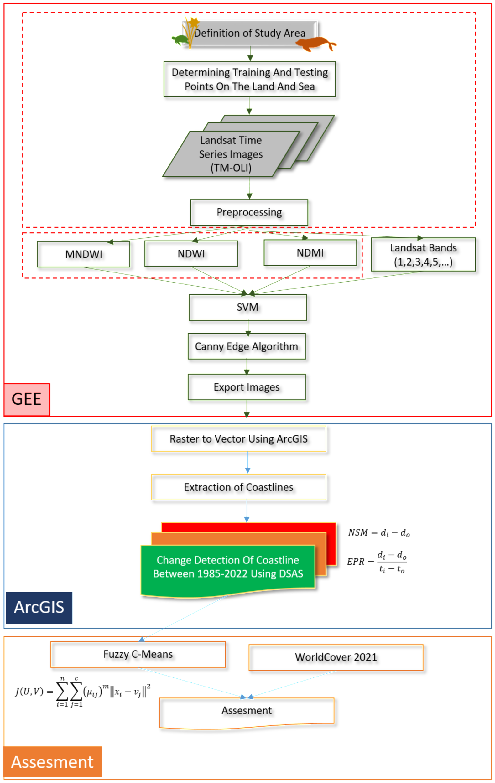
Flowchart of the study.
2.1 Study area
The study area, covering 210.83 square kilometers, lies between Göksu Incekum in Mersin Province and the Antalya provincial border. It was delineated using the polygon tool on the Google Earth Engine (GEE) platform, with special attention to the strip feature to ensure inclusion of both terrestrial and marine zones. Mersin, a major coastal city in Türkiye with a 321-kilometer shoreline, is situated along the Mediterranean Sea, along with Antalya, Adana, and Hatay. Geographically, the city spans from 32° 56’ E to 35° 11’ E and from 36° 01’ N to 37° 26’ N (Figure 2a).
Figure 2
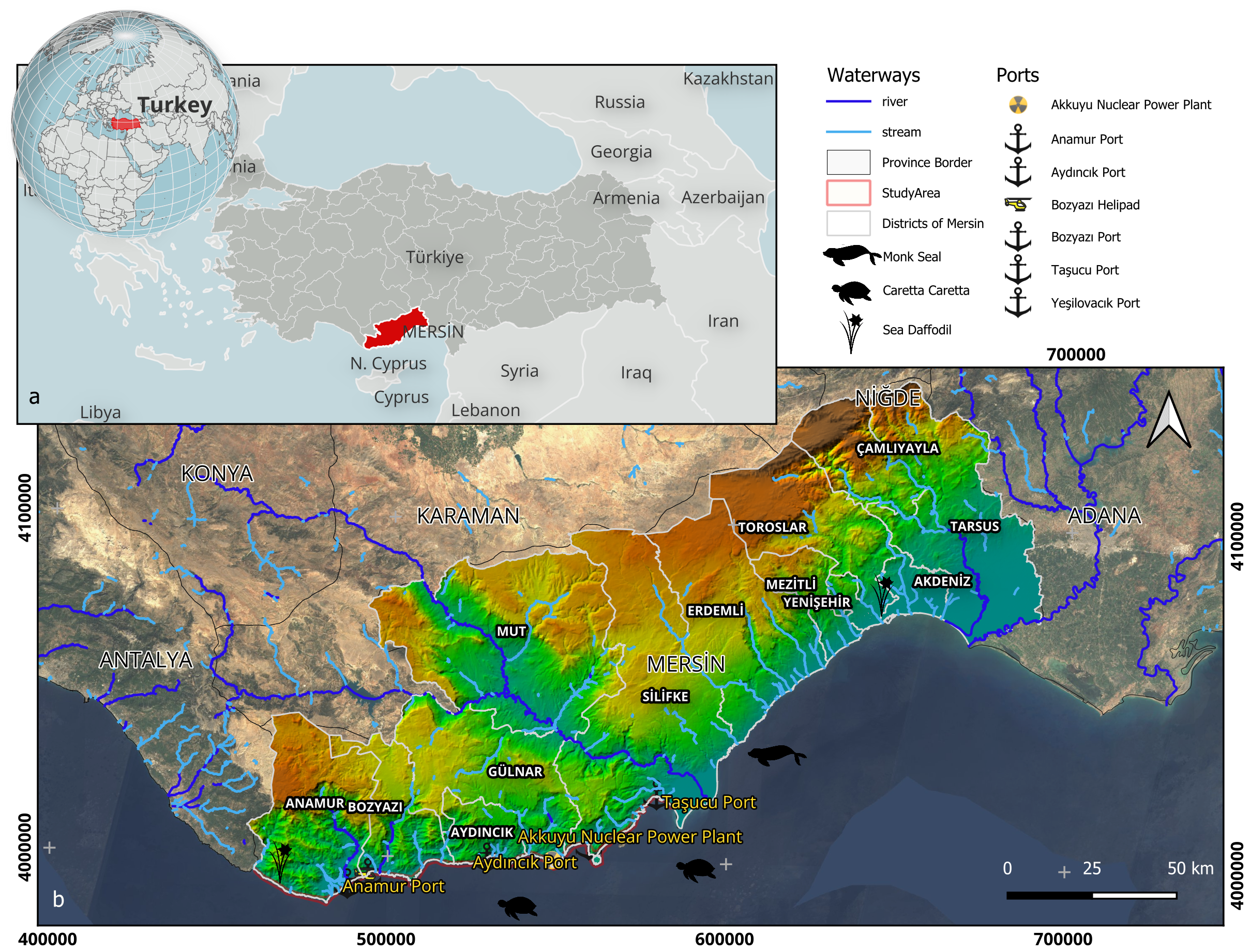
(a) Location of Mersin province in Türkiye shoreline and (b) The study area and shoreline, which includes locations where man-made objects such as nuclear power stations and ports are located, as well as Sand Lily growing areas, important accommodation areas for Mediterranean Monk Seals and Caretta Caretta Turtles.
Figure 2b illustrates the shoreline and district boundaries within the study area, which includes the coastal districts of Silifke, Gülnar, Aydıncık, Bozyazı, and Anamur. Each district exhibits distinct ecological and economic characteristics (Sakinan and Gucu, 2010; Serteser, 2018; Tel et al., 2023). The study region lies in the Mediterranean’s Taşeli Plateau, notable for its rugged coastal morphology, including cliffs, sea caves, dunes, and narrow beaches. Natural processes such as tectonic activity, lithological variation, riverine input, and climatic influences have significantly shaped the beaches between Silifke and Anamur. The bays surrounding Yeşilovacık in the Silifke district serve as key breeding habitats for the endangered Mediterranean monk seal. Silifke is connected to popular tourist areas like Susanoglu and Taşucu. Taşucu Port, an international maritime facility, began operations in 1984, paused in 2009, and resumed in 2017. The Akkuyu Nuclear Power Plant—Türkiye’s first nuclear energy facility—is located in the Gülnar district, near the town of Büyükeceli. Bozyazı’s coastline also supports a vital colony of Mediterranean monk seals, while Anamur beach provides nesting grounds for the endangered loggerhead sea turtle (Caretta caretta) (Ergüden and Ayas, 2021) (Figure 2).
2.2 Data sets
2.2.1 Remote sensing data
The initial stage of this research involved selecting and processing appropriate satellite imagery to extract coastline data. Landsat satellite images, operational for over four decades, were employed to analyze changes along Mersin’s western coastline. Landsat imagery is widely used due to its extensive temporal and spectral resolution, despite its moderate 30-meter spatial resolution (Pardo-Pascual et al., 2018; Bishop-Taylor et al., 2021). Moreover, Landsat’s shortwave infrared (SWIR) and near-infrared (NIR) bands offer high accuracy in delineating land-water boundaries (Pardo-Pascual et al., 2018). Landsat imagery was selected for this study due to its long-term continuity, broad spatial coverage (Liu et al., 2017), cost-free accessibility (Elnabwy et al., 2020), and seamless integration with the GEE platform.
Landsat satellite imagery from 1985 to 2022 was obtained from the Google Earth Engine (GEE) collection to analyze shoreline changes along the western coast of Mersin Province. Using GEE’s code editor, spatial and temporal filters were applied to conduct targeted analyses. The GEE platform enables a wide range of operations—including image processing, band ratioing, and classification—through user-defined algorithms. This study leveraged these capabilities to examine imagery from Landsat 5 TM, Landsat 7 ETM+, and Landsat 8 OLI, utilizing all available spectral bands except the thermal and panchromatic bands.
To evaluate potential tidal conditions in the study area, sea level data from the Erdemli tide gauge station (2004–2009) were analyzed. The lowest annual mean sea level was recorded in 2007 at 6960 mm, and the highest in 2009 at 7020 mm, indicating a 60 mm interannual variation. The uncertainty associated with these measurements was calculated as 1.4 mm (Holgate et al., 2013; Permanent Service for Mean Sea Level (PSMSL), 2025). Other studies in the Eastern Mediterranean report seasonal sea level variations between 3.0 and 16.6 cm, and semi-annual variations from 1.8 to 3.2 cm. Interannual changes are primarily driven by sea surface temperature fluctuations (Simav et al., 2008). Although tidal effects in the Mediterranean are generally minimal (± 0.2–0.3 m), sea level may fluctuate by up to ±0.5 m due to barometric pressure variations (Çiner et al., 2009). Because of the variable acquisition times of Landsat imagery, it was not possible to directly account for tidal variations. However, given the region’s minimal tidal range, their impact is considered negligible. To further reduce potential tidal influence related to inconsistent image acquisition times, a multi-year mean shoreline was used.
2.2.2 ESA WorldCover 2021 dataset
To assess land cover characteristics, the 2021 ESA WorldCover dataset with a 10-meter spatial resolution was employed. The dataset identifies eleven land cover classes, including tree cover, shrubland, grassland, cropland, urban areas, and mangroves, with an overall accuracy of 77%. The data are provided in an ellipsoidal WGS 1984 coordinate system (EPSG:4326), assuming a terrestrial radius of 6,378 km (Zanaga et al., 2022).
2.3 Methods
The methodology employed in this study is presented comprehensively through a flowchart (Figure 1). Flowchart illustrates the sequence of steps and procedures used during the study.
2.3.1 Receiving data and processing using the GEE platform
GEE was actively used in the first part of the study. The study utilized Google Earth Engine (GEE) for image downloading, index computation, classification, and Canny edge detection. GEE is a non-profit tool that analyzes and visualizes geospatial data sets using scientific methodologies. It archives satellite images and makes them available to the public. GEE supports Python and JavaScript for server queries and a graphical user interface for application development. It is ideal for large-scale, long-term research projects using petabyte amounts of remote sensing data (Gorelick et al., 2017). Processing satellite images and presenting the results is faster and easier when using cloud-based technological support systems like GEE. There are no limitations on time, space, or hardware with these platforms.
Landsat images from the years 1985, 1990, 1995, 2000, 2005, 2010, 2013, 2015, 2020, and 2022 were acquired using the GEE platform, with a cloud cover threshold of less than 5%, with the mean values of the 12-month images for each specified year applied. Four stages are necessary for preparing the dataset. We established the boundary of the study area using the polygon construction functionality of the GEE platform. The research area is 210.83 square kilometers, reaching the Antalya provincial boundary, and it has a balanced land and sea region (Figure 2).
Each dataset encompassed in the study spans from January 1 to December 31. Landsat 5 TM satellite images were used in 1985, 1990, and 1995, whereas Landsat 7 satellite imagery was employed in 2000. Images of the research region exhibit data loss resulting from the Landsat 7 sensor malfunction that transpired post-2003. Landsat 5 TM was utilized again in 2005 and 2010 because of its exceptional efficacy in delineating the shoreline. Landsat 8 OLI satellite images have been utilized since 2013. Several satellite pictures in the datasets underwent cloud masking prior to the delineation of the research region. The average values of the acquired photos were utilized as the resultant image for each year. The assistance of GEE has facilitated a significantly expedited progression of the processes. In the 1985 study, 5,478 photographs were processed in the cloud within seconds, followed by clipping of the application region, application of the classification technique, and use of the edge algorithm to generate the final pictures.
2.3.2 Obtaining indices to support the separation of land and sea
The primary focus of the study, coastal edge line detection, was explored in the literature, and it was found that many indices, including the Normalized Difference Water Index (NDWI) (Goksel et al., 2020; Almeida et al., 2021; Patel et al., 2021), the modified NDWI (MNDWI) (Adebisi et al., 2021), the Automated Water Extraction Index (AWEI), and the Automated Water Extraction Index (WRI), are utilized to distinguish between land and water areas. As emphasized in the studies on shoreline extraction, these indices can be used directly or to support the classification process for the separation of water and land in satellite imagery.
NDWI is a method used to identify open water areas in remotely sensed images, providing estimates of water body visibility (McFeeters, 1996). It uses a band ratio approach, producing grayscale pictures with positive values for water features and negative values for non-water features, which can be represented by Equation 1.
MNDWI effectively reduces and even eliminates built-up land noise, vegetation, and soil noise, while also enhancing open water features (Xu, 2006).
MNDWI formulation can be expressed in Equation 2.
When determining the water content of vegetation, NDMI is frequently utilized. It is computed using Equation 3 as the ratio of NIR to MIR values.
This work calculates the mean of the filtered image collection for a single year, thereafter deriving the NDWI, MNDWI, and Normalized Difference Moisture Index (NDMI) indices using GEE. This study utilized all indicators to validate the accuracy of the categorization process.
To enhance classification accuracy and facilitate the delineation of the sea and land regions, we calculated the mean values of NDWI, MNDWI, and NDMI pictures for each year individually. The resultant datasets were subsequently clipped for application in the SVM analysis and classification procedure.
2.3.3 Classification using supervised machine learning
Using the JavaScript programming language, GEE supports complex analysis. One of the specialized libraries available on the GEE platform is ‘Classifier’. This library provides various classification methods. Using typical machine learning algorithms, the classifier package manages supervised classification on Earth Engine. CART, Random Forest (Arjasakusuma et al., 2021; Zorlu, 2022), Naive Bayes, and SVM (Santra et al., 2023) classifiers were used for coastal works. SVM uses range maximization, simplifying classification by projecting the dataset onto a lower-dimensional feature space. This method is commonly used in land cover classification, particularly for binary categorization of land and water. SVM was preferred because it covers a small area, has a small dataset, involves fewer computational operations and provides good results when supported by other indices. The general classification workflow on the GEE platform is the same as that for a classical SVM. First, training data is collected. Next, a classifier is created. Using the training data, the classifier is trained.
The SVM classification technique was employed to delineate the shoreline by categorizing point data into two separate classes: sea and land. Training and test data were independently gathered for each region to guarantee precise categorization. The spots were meticulously chosen to ensure uniformity within the research region. To enhance the study’s accuracy, we quantified the data according to the sample size. The designated region has around 230,000 pixels, with each Landsat pixel measuring 900 square meters. A population of 230,000 with a sample size of 1,078 yields a 99.9% confidence level and a 5% margin of error. The study meticulously examined a sample size of 1050 training and test data, comprising 525 data points for both water and land, all delineated within the study region (Figure 3a). The study’s dataset was partitioned into training and validation subsets. The training set constituted 75% of the entire data, with the other 25% designated as test data utilizing the GEE library.
Figure 3
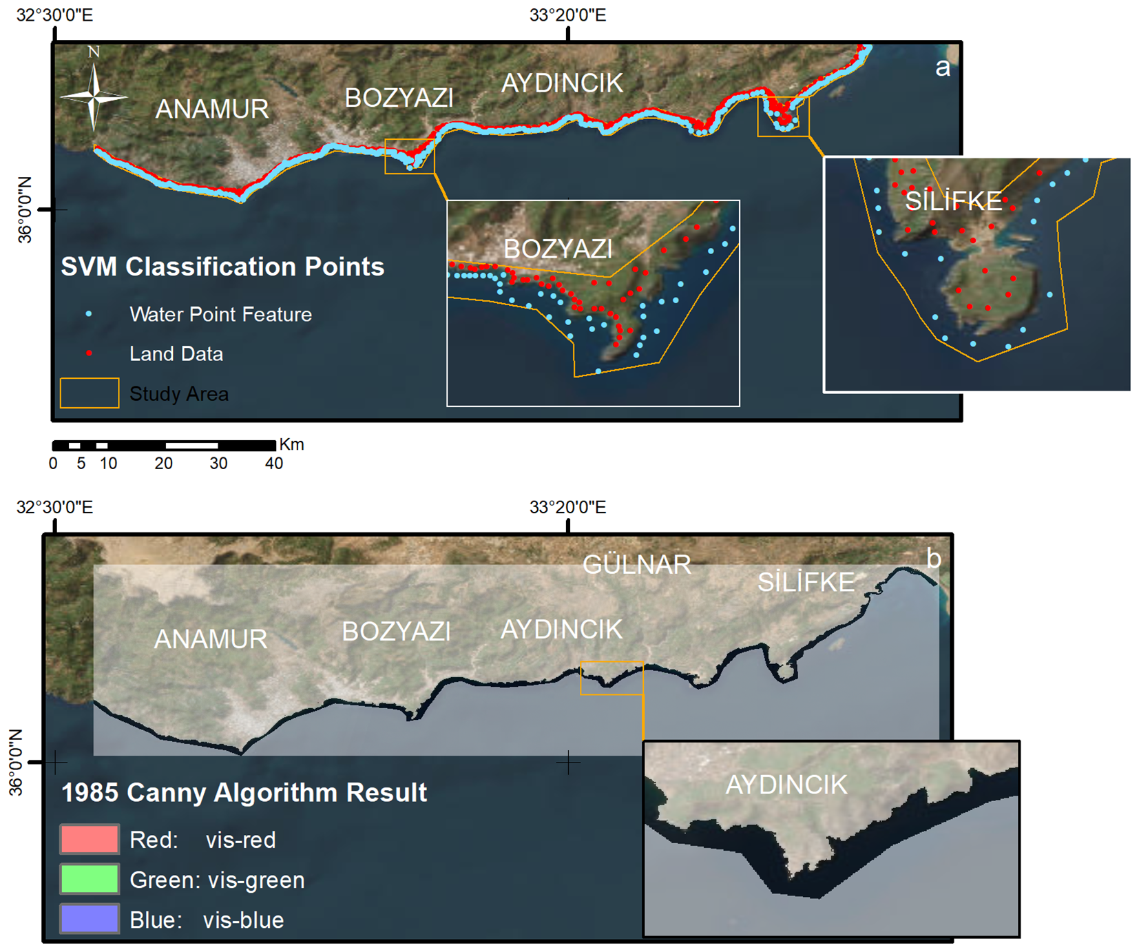
GEE Process, (a) SVM classification points, (b) Example of Canny Algorithm Result.
The research employed the SVM method, facilitated by GEE, especially ee.Classifier.libsvm within the GEE framework, to identify shorelines. We identified random points for each research year and then evaluated the accuracy. The results indicate an accuracy of 0.997 for 1985 and 1990, 1.000 for 1995, 2000, 2005, and 2010, and 0.998 for 2013, 2015, 2020, and 2022.
2.3.4 Shoreline extraction using Canny edge detection
Coastal acquisition investigations with satellite images utilize edge-detection techniques, which employ diverse mathematical methods to delineate item outlines in images. Experts have established numerous edge-detection methodologies, such as Canny, Deriche, Differential, Sobel, Prewitt, and Roberts Cross. Although Sobel, Prewitt, and Roberts methods are simple and accessible, their significant vulnerability to picture noise may result in erroneous coastline detection. The Canny method offers reliable edge identification in noisy pictures; nevertheless, it is more computationally complex and time-consuming compared to alternative techniques. Compared to other gradient-based edge detection operators, the Canny method provides better edge continuity and fewer discontinuities, making it easier to see the coastline. Its exceptional precision, particularly at maritime and terrestrial boundaries, is a primary basis for its preference in research (Colak, 2024).
The study of 98 test samples showed that Canny edge detection gives much more accurate results, especially when it comes to telling the difference between natural shorelines and developed areas (O’Sullivan et al., 2023a). The primary benefit of the Canny edge detection method is its ability to identify a broad spectrum of edges and provide detailed, accurate edge maps, enabling a clear delineation of the coastline. The Canny edge identification technique is applicable to both multispectral satellite data and SAR radar imaging for delineating the border between land and water regions (Zollini et al., 2019). The effectiveness and calculation time of the Canny method are affected by changeable factors such as Gaussian filter size and threshold. Minor filters mitigate blurring, elevated thresholds result in data loss, while diminished thresholds induce noise and superfluous data. It can accurately delineate the boundary between ice and ocean in extreme environments like Antarctica. The Canny method is distinguished by its adaptive thresholding technique, which mitigates noise and enhances edge accuracy (Yu et al., 2019). We employed the Canny method in this investigation due to its benefits.
The GEE platform endorses the Canny library, which this study utilized. The GEE platform provides many solutions for seamless edge extraction. Experiments were performed to identify the coastal-edge line alone, and the minimal values for both parameters were established (GEE, 2024).
The delineation of the coastline is a crucial aspect of the study; thus, the threshold and sigma values were selected to be minimal. We attained superior results by employing values of 0.01 and 0.05 (Figure 3b).
Thereafter, the use of the Canny technique, the images were vectorized utilizing ArcGIS. All shoreline vectors were manually inspected individually. Manual adjustments were applied minimally, especially in nearshore rocky areas or highly complex shoreline geometries. Additionally, in this study, a manual shoreline digitization was performed using 2014 orthophoto images with a spatial resolution of 0.45 m x 0.45 m, and the precision of shoreline delineation was evaluated. The research included potential inaccuracies resulting from hand digitizing. The close tool was utilized to examine proximity values, and the average proximity findings were computed. Root Mean Square Error (RMSE) values were calculated to assess accuracy. Due to the lack of additional orthophotos, we limited the evaluation of coastline accuracy to the year 2013. For the study, points were positioned at 5-meter intervals along both the manually digitized shoreline from the orthophoto and the Landsat-derived shoreline for 2013. An analysis of the closeness of the two datasets indicated an average distance of 11.45 meters between the shorelines, accompanied by a root mean square error (RMSE) of 14.71 meters.
2.3.5 Shoreline change detection using Digital Shoreline Analysis System
The ability to detect, analyze, and predict changes in the shoreline over time is critical for coastal monitoring, management, and analysis. Researchers employ both human and automated methodologies to study coastal changes. The Digital Shoreline Analysis System (DSAS) software is one automated method for analyzing these alterations. Rob Thieler and Bill Danforth created the DSAS program in the early 1990s, and it has since undergone several revisions and enhancements (DSAS 5.1, 2021).
DSAS, a free software package, is incorporated into the ESRI Geographic Information System (ArcGIS). The current version, which is also favored in the research, is 5.1, which runs on Windows 7 and Windows 10 and supports ArcGIS 10.4 to 10.7. DSAS allows users to construct rate-of-change statistics using a time series of vector shoreline locations. The Digital Shoreline Analysis System automates the process of creating measurement locations, performing rate calculations, providing statistical data required to determine rate reliability, and including a beta model for projecting shoreline position. Transects generated by DSAS are set out alongshore at a user-specified spacing and cast perpendicular to the reference baseline. The reference baseline can be constructed between historical shoreline positions or wholly on one side of the coastal data; there are no restrictions on its location. DSAS calculates change metrics like the Shoreline Change Envelope (SCE), Net Shoreline Movement (NSM), End Point Rate (EPR), Linear Regression Rate (LRR), Weighted Linear Regression Rate (WLR), Confidence Interval (LCI/WCI), Standard Error (LSE/WSE), and R-squared (LR2/WR2). It does this by measuring the length of a transect between the baseline and each shoreline intersection. It also combines date information and positional uncertainty for each shoreline (Himmelstoss et al., 2021).
The distance between the oldest and youngest shorelines is used to compute the NSM statistic; therefore, units are in meters. The NSM was calculated using Equation 4.
Where; : The youngest shoreline distance (m), : The oldest dated shoreline distance (m).
The shoreline shows seaward silting with an advancing shoreline when the NSM value is positive. Conversely, a negative NSM value causes the shoreline to retreat and erode in the direction of the land. Several studies have utilized NSM to monitor coastal changes. For example, in the study conducted for the Jiangsu coastal area, NSM values in the region were analyzed. Accordingly, it was determined that the coastlines advanced toward the sea during the 45-year period (Song et al., 2021). NSM values were also found to provide usable results in future forecasting studies (Rezaee et al., 2019).
If the distance between the oldest and the newest shoreline is divided by time, this is expressed as the EPR statistic. The EPR was calculated using Equation 5.
Where; : The youngest shoreline distance (m), : The oldest dated shoreline distance (m), : The youngest shoreline time (year), : The oldest dated shoreline time (year).
The EPR’s principal advantages are its straightforward computation and its requirement for only two shoreline data points. The primary disadvantage is that when more than two shorelines are available, the information on shoreline behavior provided by additional shorelines is disregarded. Consequently, fluctuations in the direction, magnitude, or cyclical characteristics of shoreline movement trends may remain undetected. Notwithstanding this limitation, EPR is significantly favored in research. It is mostly utilized to identify temporal erosion and accretion (Baig et al., 2020).
The LRR statistic is a rate of change metric computed by DSAS. It denotes the mean rate of shoreline displacement over a certain duration. The least squares approach was employed to determine the line. This strategy, in contrast to others, considers all shorelines utilized in the research. The time indicated refers to the year of the shorelines, and the variable designated as distance represents the measurement from the start of the main line to the point of intersection with the shorelines for each transect. The gradient of the produced line indicates the pace of coastal alteration. For this reason, it is a more sensitive method than other methods of calculating the rate of shoreline change. It is preferred in coastal erosion studies (Rezaee et al., 2019), beach management, effects of sea level rise (Adebisi et al., 2021), climate change assessments (Johnson et al., 2015).
LRR equation can be calculated using Equation 6.
Where; : Distance from the baseline in meters, : The shoreline date interval in years, : Slope of the fitted line, : The y-intercept.
The shoreline change envelope (SCE) provides a distance instead of a rate. The maximum distance among all shorelines intersecting a specific transect is denoted by the SCE value. Due to the absence of a sign in the total distance between two shorelines, the SCE value remains consistently positive. Values around zero indicate a few alterations in the coastline over the study period, attributable to the characteristics of the SCE index. This tool is very beneficial for analyzing sites that have remained constant throughout time.
Shoreline maps were initially created in shape file format with ArcGIS 10.8, aligned with the information offered by DSAS to assess shoreline changes in the research region. After preparing the shoreline maps for examination, we created a baseline layer, approximately 100 meters from the shorelines, using buffer analysis. The primary determining element in baseline production is whether the shoreline change rate should be determined using a land-based baseline or a seaside baseline. In this study, we assessed shoreline alteration based on the reference line established along the coast. After using the DSAS tool’s criteria, the coastline and reference line layers of the research area were looked at, and the rate of shoreline change was calculated. We determined the rate of shoreline change in the study region using 750 m long profile lines at 50 m intervals. A total of 3,871 profile lines were created to assess the shoreline alteration in the research region. All transects were carefully reviewed, particularly in regions with pronounced coastal indentations and narrow straits, to prevent misalignment with non-target shoreline segments. This study utilized the statistical data of the SCE, NSM, EPR, and LRR. NSM, EPR, and LRR are employed to analyze alterations in the study area, while SCE is utilized to identify and evaluate analogous pattern regions using the fuzzy C-means clustering technique alongside other statistical outcomes.
2.3.6 Fuzzy C means clustering algorithm for pattern detection of transects
Fuzzy C-means (FCM) is an effective technique for grouping unlabeled data and locating hidden structures in a data set. Fuzzy C-Means (FCM) is a popular unsupervised learning method that enhances pattern recognition and computer vision. J.C. Dunn created fuzzy c-means (FCM) clustering in 1973 (Dunn, 1973), and J.C. Bezdek improved algorithm in 1981 (Bezdek, 1981).The technique determines the membership of each data point for a cluster center based on the distance between the center and the data point, with closer points being more affiliated with the cluster center. Membership and cluster centers are adjusted based on Equations 7, 8 after every iteration:
Where; is the number of data points, represents the cluster center, is the fuzziness index represents the number of cluster center, represents the membership of data to cluster center, represents the Euclidean distance between data and cluster center.
The fuzzy c-means algorithm’s primary goal is to minimize with Equation 9:
Where; is the Euclidean distance between data and cluster center.
The study employed Konstanz Information Miner (KNIME) software for fuzzy c-means analysis, a dependable open-source platform for data analytics (KNIME AG, 2024). The approach proved proficient at identifying patterns within smaller datasets, such as the one utilized in the study. Fuzzy c-means is an efficient technique for identifying patterns in smaller datasets, such as the one used in this study, because of its straightforward framework. We used SCE, NSM, LRR, and EPR data from each transect along with fuzzy c-means clustering to find patterns in the coastline. The findings offer a definitive elucidation of the influence of human activities in the studied region.
3 Results
The GEE platform enabled efficient extraction of shoreline edges, which were subsequently digitized using ArcGIS. DSAS was then used to analyze shoreline changes in the study area from 1985 to 2022. The methods and findings are elaborated in the following sections.
3.1 Digital Shoreline Analysis System results
ArcGIS 10.8 was used to perform raster-to-vector conversions following Canny edge detection on the classified imagery. Shoreline data were generated in linear format for each year of analysis.
The statistical outputs from DSAS—NSM, SCE, LRR, and EPR—were evaluated using Pearson correlation coefficients. A strong positive correlation (r = 0.734) was observed between SCE and NSM. EPR and LRR exhibited a perfect correlation (r = 1.000), and EPR, LRR, and NSM were closely linked, with coefficients ranging from 0.941 to 1.000 across the dataset. As shown in Table 1, SCE demonstrated a moderate positive correlation with the other indicators, as expected.
Table 1
| SCE | NSM | EPR | LRR | |
|---|---|---|---|---|
| SCE | 1.000 | |||
| NSM | 0.734 | 1.000 | ||
| EPR | 0.734 | 1.000 | 1.000 | |
| LRR | 0.674 | 0.941 | 0.941 | 1.000 |
Correlation between statistical results.
Each district determined the maximum, minimum, and average values for NSM, SCE, EPR, and LRR metrics across the entire shoreline. This approach facilitated the identification of intra-district variations and highlighted areas requiring targeted monitoring. The total number of transects analyzed in Anamur, Bozyazı, Aydıncık, Gülnar, and Silifke were 807, 781, 640, 390, and 1,253, respectively.
3.1.1 NSM results
The NSM analysis revealed that 57.09% of the transects exhibited negative displacement, while 42.75% showed positive displacement, with a mean shoreline change of 1.84 meters.
Assessment of district-wise shoreline change expenditures showed that Gülnar had the highest positive variation (38.54%), while Bozyazı exhibited the largest negative variation (40.24%). Silifke demonstrated both the highest positive (12.04%) and negative (20.18%) changes relative to the total shoreline (Table 2).
Table 2
| NSM | District Border | Whole | |||||||||
|---|---|---|---|---|---|---|---|---|---|---|---|
| Max | TID | Min | TID | Mean | PC | PN | NoC | PC | PN | NoC | |
| Anamur | 206.02 | 694 | -78.79 | 730 | 3.62 | 36.20 | 31.90 | 0.00 | 11.08 | 9.76 | 0.00 |
| Bozyazı | 338.40 | 846 | -79.64 | 1154 | -5.27 | 19.51 | 40.24 | 0.00 | 6.59 | 13.59 | 0.00 |
| Aydıncık | 91.18 | 2056 | -130.63 | 2055 | 0.38 | 29.03 | 35.48 | 0.00 | 7.44 | 9.09 | 0.00 |
| Gülnar | 588.59 | 2389 | -84.76 | 2538 | 30.52 | 38.54 | 30.73 | 0.00 | 5.61 | 4.47 | 0.00 |
| Silifke | 335.33 | 2841 | -97.19 | 2961 | -3.05 | 22.84 | 38.28 | 0.29 | 12.04 | 20.18 | 0.15 |
NSM Results.
TID, TransectID; PC, Percentage of Positive Change; NC, Percentage of Negative Change; NoC, Percentage of No Change.
Shoreline lengths were determined by vectorizing satellite imagery. The longest shoreline length, 213.92 km, was recorded in 2015, while the shortest, 202.55 km, occurred in 1985 (Figure 4a). Areas with both negative and positive NSM values are displayed in Figure 4b. Notably, a negative shift was observed along the Anamur shoreline between 1985 and 2022. In contrast, the area surrounding the Akkuyu Nuclear Power Plant (ANP) experienced a marked positive NSM shift over the same period (Figure 4b).
Figure 4
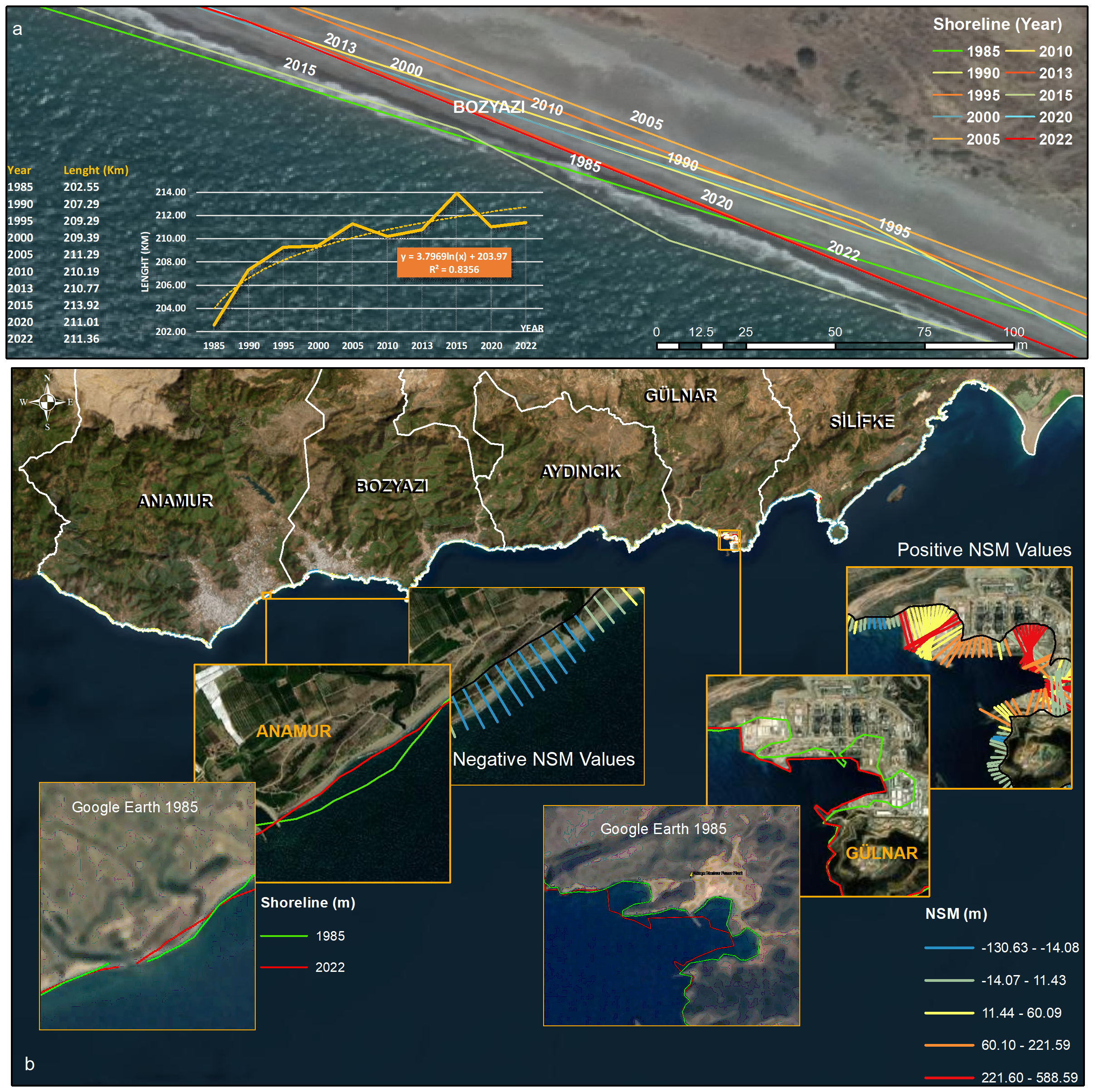
The NSM provides a comprehensive analysis of shoreline results. (a) Shorelines over the years, shoreline lengths, and graph, (b) shows NSM values on the result map of the whole study area, with examples of negative and positive NSM.
3.1.2 Shoreline lengths and SCE results
The Shoreline Change Envelope (SCE) is a key metric for detecting long-term coastal variation. The SCE analysis revealed an average shoreline shift of 31.79 meters, with extremes ranging from 0.04 meters to 595.17 meters. A column chart summarizing all transects is presented in Figure 5a. Complementary to the Net Shoreline Movement (NSM) results, a spatial map of SCE was produced to illustrate shoreline changes across the entire study area (Figure 5b). The column chart highlights pronounced variations in the districts of Gülnar, Silifke, Bozyazı, and Anamur, with minimal change observed in Aydıncık. A specific example of shoreline change is demonstrated near the Akkuyu Nuclear Power Plant (ANP), serving as a localized case study (Figure 5c).
Figure 5
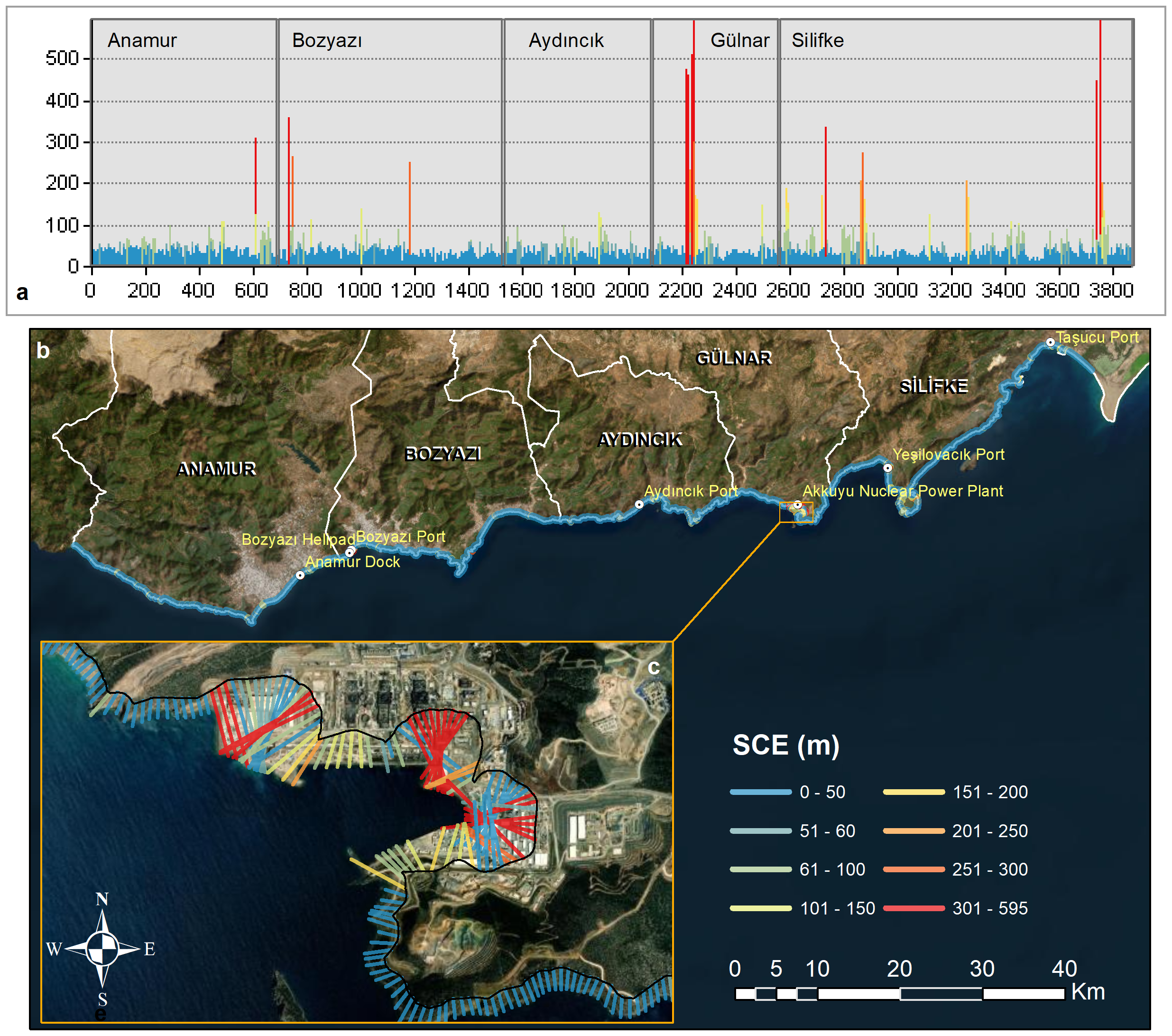
Shoreline lengths and SCE results. (a) shows the SCE values graph for transects, (b) shows the SCE values map of the entire study area, and (c) shows an example of one of the areas where the highest SCE values are observed.
3.1.3 EPR results
The study area exhibits an average End Point Rate (EPR) of 0.05 m/year, with erosion observed in 2,167 transects, accounting for 55.98% of the total.
Gülnar was most notably affected, particularly transect 2839, which recorded a high accretion rate of 15.91 m/year. Bozyazı followed with a rate of 9.15 m/year. Conversely, transect 2055 in Aydıncık and transect 2961 in Silifke showed erosion rates of −3.53 and −2.63 m/year, respectively (Table 3).
Table 3
| EPR | District Border | Whole | |||||||||
|---|---|---|---|---|---|---|---|---|---|---|---|
| Max | TID | Min | TID | Mean | PC | PN | NoC | PC | PN | NoC | |
| Anamur | 5.57 | 694 | -2.13 | 730 | 0.10 | 35.18 | 31.07 | 1.34 | 10.85 | 9.58 | 0.41 |
| Bozyazı | 9.15 | 846 | -2.15 | 1154 | -0.14 | 18.87 | 39.65 | 0.91 | 6.41 | 13.46 | 0.31 |
| Aydıncık | 2.46 | 2056 | -3.53 | 2055 | 0.01 | 28.26 | 34.57 | 1.30 | 7.28 | 8.91 | 0.34 |
| Gülnar | 15.91 | 2389 | -2.29 | 2538 | 0.83 | 37.81 | 30.21 | 0.88 | 5.53 | 4.42 | 0.13 |
| Silifke | 9.06 | 2841 | -2.63 | 2961 | -0.08 | 21.36 | 36.76 | 2.57 | 11.39 | 19.61 | 1.37 |
EPR results.
TID, TransectID; PC, Percentage of Positive Change; NC, Percentage of Negative Change; NoC, Percentage of No Change.
District-level shoreline comparisons revealed that Gülnar experienced the most favorable transformation, with a 37.81% positive change. Bozyazı recorded the most significant adverse change at 39.65%. In Silifke, the highest positive (11.39%) and negative (19.61%) changes were observed, although 1.37% of its shoreline remained unchanged.
EPR and LRR values were classified according to the scale proposed by (Emam and Soliman, 2020) (Table 4).
Table 4
| Shoreline Classification | Rate of Change (m/year) |
|---|---|
| Very High Erosion | <-2 |
| High Erosion | <-1→≥-2 |
| Moderate Erosion | <0→≥-1 |
| Stable | 0 |
| Moderate Accretion | >0→≤+1 |
| High Accretion | >1→≤+2 |
| Very High Accretion | >+2 |
Shoreline EPR and LRR classification (Emam and Soliman, 2020).
Using this classification, a bar graph (Figure 6a), EPR maps covering the entire shoreline (Figure 6b), and district-specific EPR tables (Table 5) were generated. As examples, Figure 6c shows a high-erosion area in Anamur; Figure 6d highlights very high accretion zones in Gülnar; and Figure 6e illustrates moderate accretion areas in Silifke.
Table 5
| LRR | District Border | Whole | |||||||||
|---|---|---|---|---|---|---|---|---|---|---|---|
| Max | TID | Min | TID | Mean | PC | PN | NoC | PC | PN | NoC | |
| Anamur | 5.57 | 694 | -1.81 | 727 | 0.26 | 55.34 | 21.75 | 0.58 | 14.85 | 5.84 | 0.15 |
| Bozyazı | 5.02 | 1314 | -1.8 | 1154 | 0.00 | 27.72 | 34.59 | 1.55 | 8.76 | 10.93 | 0.49 |
| Aydıncık | 2.61 | 1883 | -1.96 | 2055 | 0.05 | 44.96 | 26.39 | 1.13 | 10.26 | 6.02 | 0.26 |
| Gülnar | 15.47 | 2389 | -1.27 | 2376 | 0.73 | 53.24 | 21.02 | 2.36 | 7.00 | 2.76 | 0.31 |
| Silifke | 9.72 | 2841 | -2.80 | 2993 | 0.05 | 39.84 | 28.57 | 1.51 | 18.44 | 13.23 | 0.70 |
LRR results.
TID, TransectID; PC, Percentage of Positive Change; NC, Percentage of Negative Change; NoC, Percentage of No Change.
Figure 6
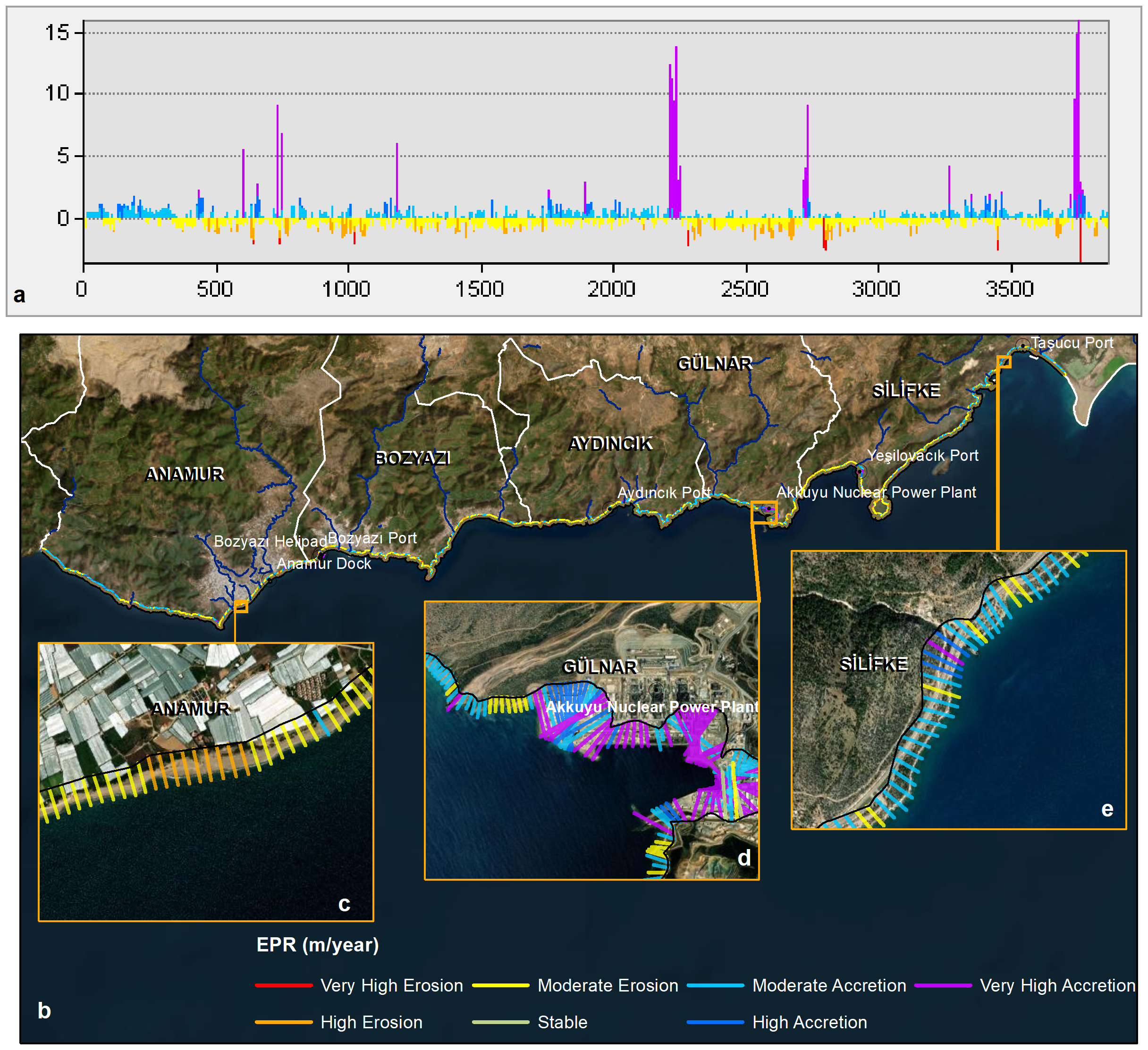
EPR, results of shorelines. (a) shows EPR erosion and accretion values graph for each transect, (b) shows EPR values of the whole study area result map, and (c–e) show examples of maps of regions that show remarkable results.
3.1.4 LRR results
Accretion was identified in 2,296 LRR transects, accounting for 59.31% of the total shoreline.
These classified values were used to generate a column graph (Figure 7a), comprehensive LRR maps of the entire shoreline (Figure 7b), and a district-specific results table (Table 5). Regional erosion and accretion patterns are also visualized: erosion in Anamur (Figure 7c) and Silifke (Figure 7e), and accretion in Gülnar (Figure 7d).
Figure 7
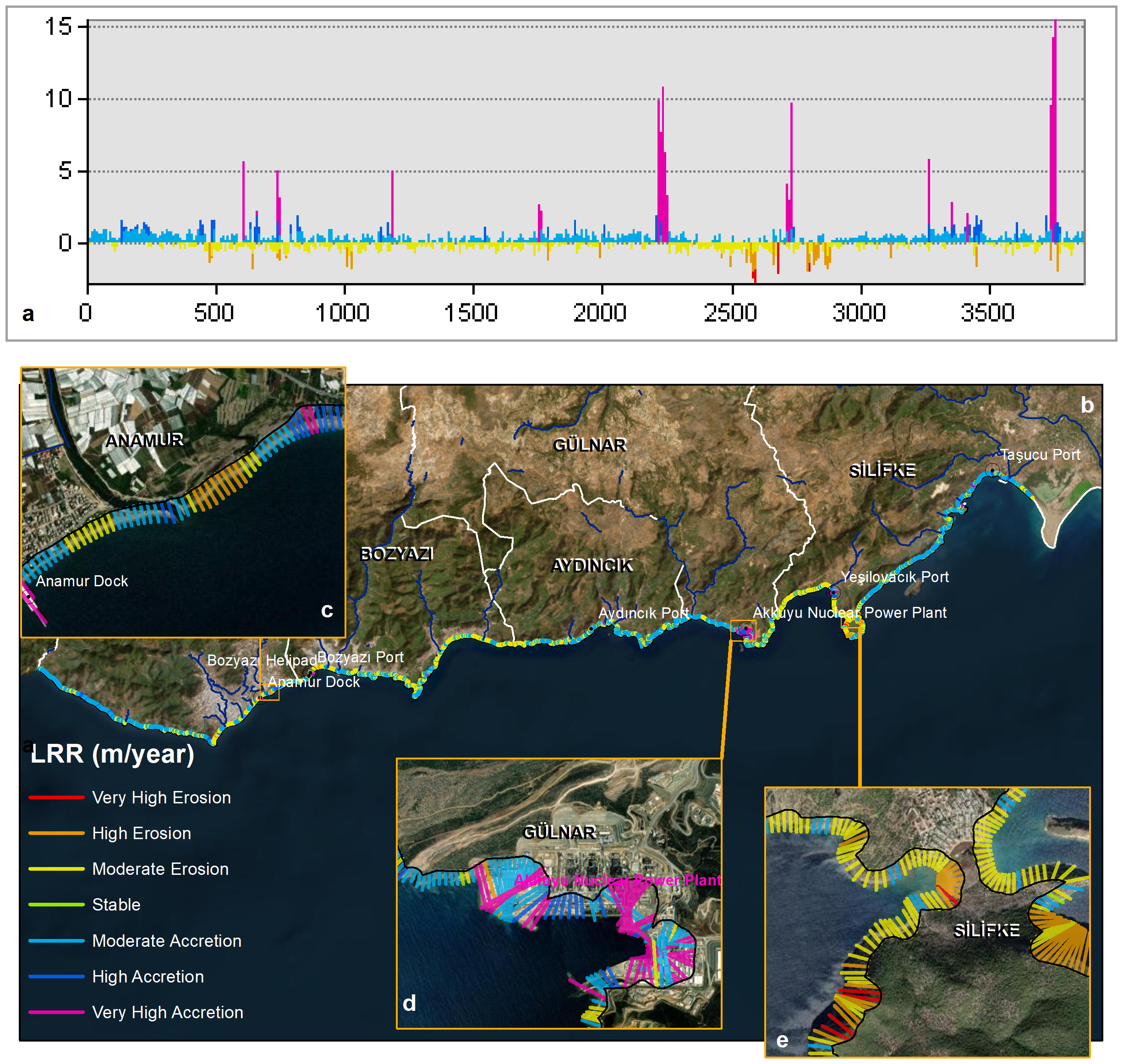
LRR, results of shorelines. (a) shows LRR erosion and accretion values graph for each transect, (b) shows LRR values of the whole study area result map, and (c–e) show examples of maps of regions that show remarkable results.
The data indicate that Transect ID 2389, with a positive LRR of 15.47 m/year, significantly affects the Gülnar district. This is followed by Silifke (9.72 m/year) and Transect ID 2841. In contrast, Silifke (Transect ID 2993) shows a negative LRR of -2.80 m/year, while Aydıncık (ID 2055) records -1.96 m/year, indicating adverse effects. Among all districts, Anamur exhibited the highest proportion of positive shoreline change (55.34%), whereas Bozyazı experienced the most pronounced negative change (34.59%).
At the broader coastal scale, Silifke shows both the largest share of positive (18.44%) and negative (13.23%) change.
Analysis of EPR and LRR values (Tables 3, 5) reveals a consistent trend: the proportion of negative changes exceeds positive changes across most districts and for the entire shoreline. This discrepancy stems from the methodological differences between LRR and EPR. LRR, which incorporates all shoreline positions over time, captures a more stable long-term trend. In contrast, EPR reflects only the change between two endpoints and is more susceptible to short-term variability. As a result, LRR offers a more reliable representation of long-term coastal dynamics, particularly relevant to the evolving shorelines of Aydıncık, Gülnar, and Silifke. To further examine this trend, comparative graphs of EPR and LRR classes were generated for the entire coastline and its neighboring areas (Figure 8). Overall, moderate accretion emerges as the dominant process.
Figure 8
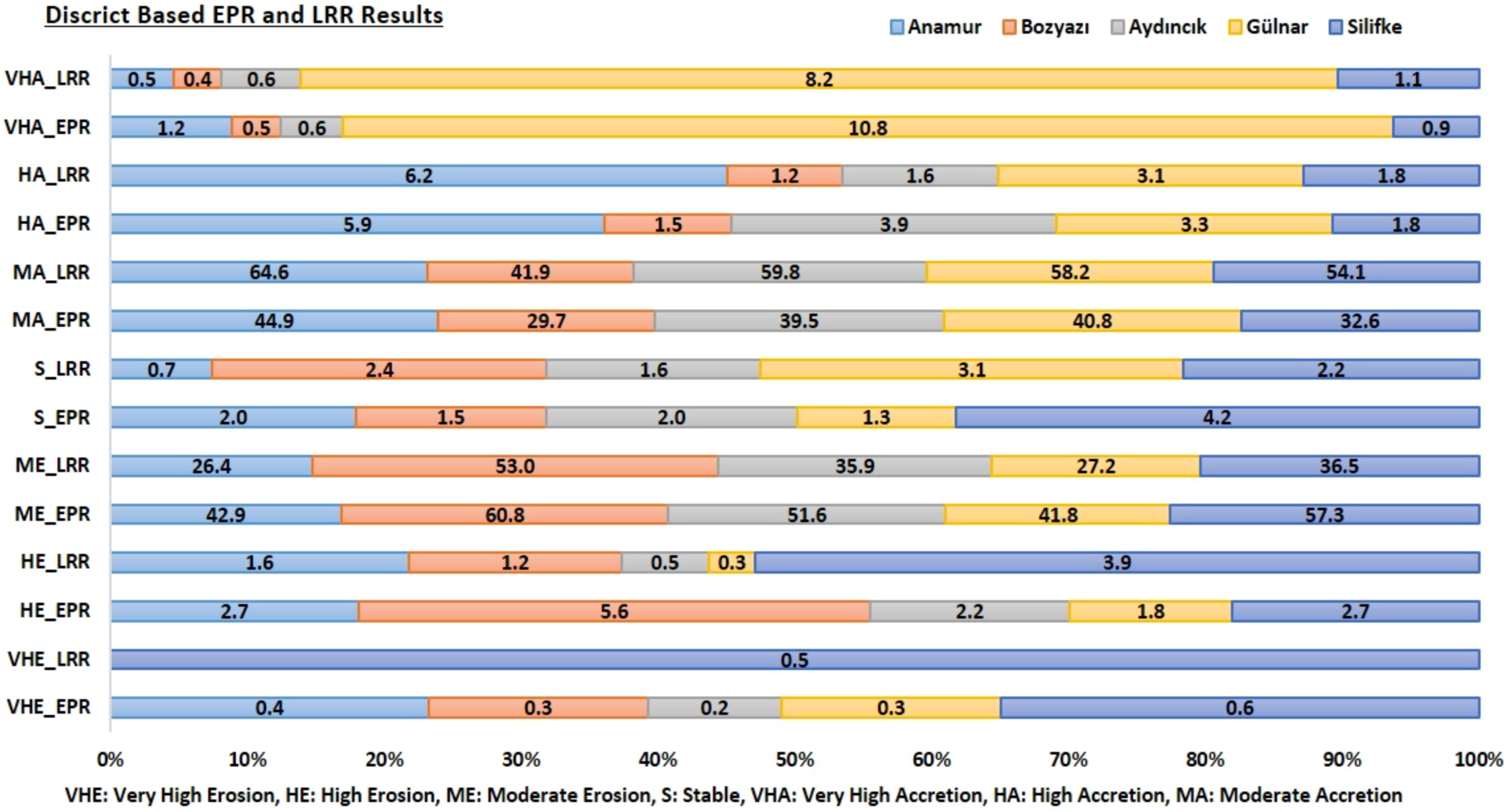
EPR and LRR results of districts.
Following classification using Table 4, the correspondence between EPR and LRR results was evaluated at the transect level. Matching rates for the entire shoreline were 67.84% in Anamur, 70.26% in Bozyazı, 71.57% in Aydıncık, 66.72% in Gülnar, 67.95% in Silifke, and 64.49% overall. As mention before the variation in matching rates is attributed to methodological differences: LRR utilizes regression across all shoreline positions, while EPR calculates change based solely on two time points. Notably, both methods indicate that extensive accretion exceeds extensive erosion across the entire coast. However, this aggregate trend complicates definitive classification of the overall shoreline status. A more granular, segmented assessment is necessary for meaningful interpretation.
According to EPR and LRR results (Figure 8), Gülnar exhibits the highest accretion rates—10.8% for EPR and 8.2% for LRR—among all districts. Silifke shows the highest erosion rates, at 0.6% (EPR) and 0.5% (LRR), followed by Bozyazı with 5.6% erosion (EPR) and Silifke again with 3.9% (LRR). In Bozyazı, mild degradation dominates in both datasets. The distribution graph of EPR and LRR classes confirms that moderate accretion and moderate erosion are the most prevalent categories along the inter-district coastline.
3.2 Land use land cover and fuzzy C-means analysis
This section of the study consists of two main phases. First, DSAS statistical outputs were synthesized to characterize shoreline change patterns. Second, these spatial clusters were examined in the context of broader land use trends.
The FCM methodology analyzes statistical data generated by the DSAS software to identify spatial and temporal trends within the study area. The methodology was implemented using KNIME, which processed standardized NSM, SCE, EPR, and LRR values (scaled between 0 and 1) as input. The optimal number of clusters was determined using the Silhouette score, calculated for varying cluster quantities. The highest Silhouette score indicated the most appropriate cluster count, which was found to be four. These clusters were labeled C0, C1, C2, and C3. Clustering was performed with a maximum of 99 iterations to limit runtime for complex datasets. A fuzziness parameter of 2 was selected to control the degree of ambiguity in the clustering process. The silhouette coefficient, which ranges from –1 to +1 and indicates clustering quality, was calculated for each result. An overall average silhouette score of 0.693 suggests strong clustering performance. Individual silhouette coefficients for clusters C0, C1, C2, and C3 were 0.689, 0.697, 0.684, and 0.765, respectively, indicating well-separated and internally cohesive clusters.
A graph illustrating the clusters assigned to each transect was generated to visualize the clustering outcomes (Figure 9a). Land use status at each location was determined by assigning each transect, which served as the basis for subsequent analysis. The results indicate that 34.40% of the study area falls under ESA code 10, representing regions dominated by tree cover. Grassland areas, classified under code 30, account for 21.87% and are primarily characterized by natural shrub vegetation. Regions with bare or sparse vegetation—defined as having no more than 10% plant cover throughout the year and dominated by exposed soil, sand, or rock—make up 16.65% of the dataset. Built-up areas, including infrastructure such as buildings, roads, and railways, represent 8.98% of the total land area.
Figure 9
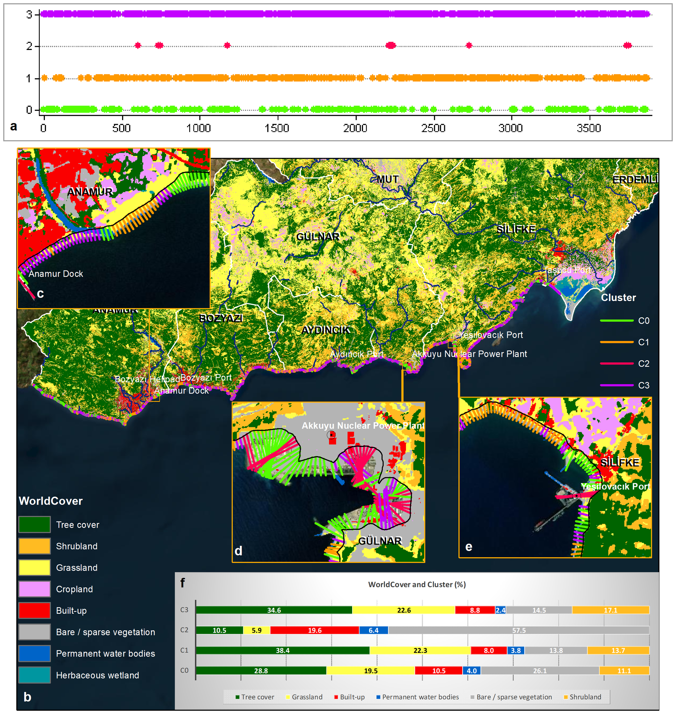
Fuzzy c-means and WorldCover results of shorelines. (a) shows fuzzy c-means clusters of transects, (b) shows fuzzy c-means clusters of study area (c–e) show examples of maps of regions that show remarkable cluster results; (f) shows cluster results and WorldCover distributions.
A spatial map of shoreline cluster patterns was also generated (Figure 9b). High-density areas are concentrated in clusters C0, C1, and C3, based on the transect cluster distribution. As shown in Figure 9a, cluster C2 exhibits relatively lower dispersion compared to the other clusters. The Akkuyu Nuclear Power Plant area (Figure 9d) shows high concentrations of C0 and C2, while the Silifke Taşucu Port region (Figure 9e) is dominated by C0 and C1 clusters. Cluster C1 and C3 regions correspond to less-developed coastal areas with minimal built-up features (Figure 9c).
ESA’s 2021 WorldCover dataset was used to generate a stacked bar chart (Figure 9f), presenting land use distributions across the study area and the associated cluster zones. A spatial join technique aligned cluster points and transects for accurate land use categorization. Based on the resulting pixel-level data, land use percentages were determined for each cluster.
The percentage bar graph (Figure 9f) highlights that C0 regions are characterized by grassland, bare land, and built-up coverage. Cluster C1 comprises 8.0% built-up land and 13.8% barren or partially vegetated terrain, as depicted in Figures 9c and 9e. Cluster C2 consists primarily of barren land interspersed with structures. In contrast, Cluster C3 is characterized by dense green vegetation, particularly concentrated along the Anamur coastline (Figure 9c).
The relationship between shoreline change types (erosion, accretion, stable) and land cover categories was analyzed for each cluster (C0–C3) using both End Point Rate (EPR) and Linear Regression Rate (LRR). The findings are summarized in Table 6, which presents detailed percentage distributions of land cover classes for each shoreline change type and cluster. As shown in Table 6, Cluster C1 is most strongly associated with erosion, particularly under EPR, where it contains high proportions of tree cover (37.86%), grassland (22.05%), and bare or sparse vegetation (13.73%). Similar trends are seen with LRR values, though slightly lower, indicating the persistence of these natural cover types in eroding regions. Cluster C3, also linked to erosion, includes substantial tree cover (18.07%) and grassland (11.26%), reflecting a pattern of erosion in less-developed vegetated coasts. In contrast, Cluster C2 is clearly associated with accretion, exhibiting 57.53% bare/sparse vegetation and 19.63% built-up land in both EPR and LRR, signaling coastal growth in highly disturbed or artificial landscapes. Cluster C0 also appears frequently in accreting areas, characterized by a mix of tree cover (28.57%), grassland (19.18%), and bare land (25.77%), implying semi-natural buffer zones. Stable shoreline segments are sparse across all clusters and land cover types, with the majority of values falling below 1.5%, highlighting the overall dynamism of the coastal environment in the study area.
Table 6
| EPR | LRR | ||||||||
|---|---|---|---|---|---|---|---|---|---|
| C0 | C1 | C2 | C3 | C0 | C1 | C2 | C3 | ||
| Erosion | Tree cover | 0.27 | 37.86 | 0.00 | 18.07 | 0.21 | 34.42 | 0.00 | 9.27 |
| Shrubland | 0.18 | 13.53 | 0.00 | 8.55 | 0.14 | 11.05 | 0.00 | 3.89 | |
| Grassland | 0.25 | 22.05 | 0.00 | 11.26 | 0.50 | 19.14 | 0.00 | 6.43 | |
| Built-up | 0.25 | 7.97 | 0.00 | 4.41 | 0.11 | 7.47 | 0.00 | 2.96 | |
| Bare/sparse vegetation | 0.21 | 13.73 | 0.00 | 6.31 | 0.30 | 12.08 | 0.00 | 3.75 | |
| Permanent water bodies | 0.05 | 3.77 | 0.00 | 1.11 | 0.07 | 3.60 | 0.00 | 0.96 | |
| Accretion | Tree cover | 28.57 | 0.38 | 10.50 | 15.12 | 28.64 | 3.74 | 10.50 | 24.00 |
| Shrubland | 10.88 | 0.18 | 0.00 | 7.76 | 10.93 | 2.54 | 0.00 | 12.93 | |
| Grassland | 19.18 | 0.19 | 5.94 | 10.29 | 18.99 | 2.94 | 5.94 | 15.60 | |
| Built-up | 10.29 | 0.03 | 19.63 | 4.13 | 10.42 | 0.53 | 19.63 | 5.64 | |
| Bare/sparse vegetation | 25.77 | 0.04 | 57.53 | 7.64 | 25.80 | 1.49 | 57.53 | 10.50 | |
| Permanent water bodies | 3.92 | 0.06 | 6.39 | 1.20 | 3.89 | 0.24 | 6.39 | 1.41 | |
| Stable | Tree cover | 0.00 | 0.15 | 0.00 | 1.38 | 0.00 | 0.24 | 0.00 | 1.30 |
| Shrubland | 0.00 | 0.00 | 0.00 | 0.74 | 0.00 | 0.12 | 0.00 | 0.23 | |
| Grassland | 0.07 | 0.01 | 0.00 | 1.09 | 0.00 | 0.18 | 0.00 | 0.62 | |
| Built-up | 0.00 | 0.00 | 0.00 | 0.26 | 0.00 | 0.00 | 0.00 | 0.21 | |
| Bare/sparse vegetation | 0.11 | 0.03 | 0.00 | 0.58 | 0.00 | 0.24 | 0.00 | 0.27 | |
| Permanent water bodies | 0.00 | 0.01 | 0.00 | 0.10 | 0.00 | 0.00 | 0.00 | 0.04 | |
Clusters and EPR/LRR analysis with land cover.
While both EPR and LRR indicate consistent land cover–cluster relationships, LRR provides a more stable and reliable estimate due to its use of time series data and statistical smoothing. It effectively captures long-term trends, minimizing the impact of short-term anomalies.
4 Discussion
This study provides a historical analysis of shoreline changes, emphasizing the impacts of both anthropogenic activities and natural processes on coastal morphology. The methodology integrates the Google Earth Engine (GEE) platform, the Digital Shoreline Analysis System (DSAS), and the Fuzzy C-Means (FCM) clustering algorithm to support comprehensive monitoring of erosion and deposition patterns.
GEE proved particularly advantageous as a cloud-based platform, enabling efficient processing of extensive satellite imagery datasets. Its capabilities were essential for the long-term analysis of shoreline dynamics from 1985 to 2022. GEE’s built-in libraries facilitated the calculation of key indices—NDWI, MNDWI, and NDMI—which were directly applied using the SVM module (Santra et al., 2023) and demonstrated strong performance in shoreline delineation. Additionally, GEE’s flexibility supported the implementation of the Canny edge detection method.
The Canny edge detection algorithm, widely used for precise shoreline identification (O’Sullivan et al., 2023b, a), played a critical role in this study. By detecting subtle transitions in satellite image color gradients, the algorithm enhanced shoreline extraction accuracy and enabled the reliable identification of complex coastal features.
Changes in shoreline length over time can result from both natural and anthropogenic factors (Yu et al., 2019; Liang et al., 2023). The average shoreline length across all measured periods was approximately 209.71 km. In 2015, the shoreline had increased by about 11.37 km compared to 1985, and by 2022, it showed an increase of roughly 8.82 km.
To evaluate shoreline erosion, accretion, and length variations in greater detail, we used the Digital Shoreline Analysis System (DSAS). This widely adopted tool enables the quantitative assessment of shoreline dynamics. In this study, DSAS, along with the Shoreline Change Envelope (SCE), Net Shoreline Movement (NSM), End Point Rate (EPR), and Linear Regression Rate (LRR) methods, was employed to identify long-term trends in shoreline change. The results highlight substantial spatial variability in shoreline change rates, underscoring the importance of DSAS-based metrics for coastal management.
Coastal erosion and accretion along the districts of Aydıncık, Anamur, Bozyazı, Silifke, and Gülnar—situated on the Mediterranean coast of the Taurus Mountains—are influenced by geographical features, riverine activity, and human interventions. Coastal erosion, driven by wave action, currents, and anthropogenic impacts, results in the landward retreat of the shoreline (Kumar et al., 2010). The Mersin coastline, particularly low-lying areas such as deltas and lagoons, is especially vulnerable to sea-level rise and wave energy.
The NSM metric, which measures the shortest distance between initial and final shoreline positions, provides a preliminary indication of erosion and accretion. Analysis of NSM values shows that, overall, erosion and accretion are nearly equally distributed across transects. Despite the overall balance, certain districts—most notably Silifke and Aydıncık—exhibit significantly high negative NSM values (Table 2). Human-made coastal structures significantly influence erosion and deposition patterns. Unsurprisingly, erosion and accretion often occur near port facilities (Rezaee et al., 2019; Song et al., 2021; Amara Zenati et al., 2024; Ozturk and Maras, 2024). According to NSM data, Anamur exhibits high accretion rates. To better understand these dynamics, further investigation into sediment sources and wave-current interactions is necessary. One prominent coastal structure in the study area is the Akkuyu Nuclear Power Plant in Gülnar. Although its location was selected based on geological stability and cooling needs, previous studies have also indicated that such facilities may contribute to accelerated coastal change (Sheik and Chandraseka, 2011; Thomas et al., 2023).
The LRR analysis revealed positive values in 59.31% of transects across the entire coastline. Localized accretion was most prominent in the Gülnar and Anamur districts. In contrast, Bozyazı exhibited a predominance of negative values, indicating a net erosional trend.
EPR data (Table 3) support these findings, with significant accretion particularly evident in Gülnar (Figure 6). Coastal erosion in Silifke is exacerbated by rising sea levels and increasing wave energy. In contrast, steeper coastal gradients in regions such as Aydıncık reduce susceptibility to erosion (Aykut and Tezcan, 2024).
Accretion occurs when sediments transported by rivers are deposited in coastal zones. However, anthropogenic structures such as dams significantly disrupt natural river flow and sediment transport, often reducing sediment delivery to delta regions and exacerbating coastal erosion (Darwish and Smith, 2023). Rivers originating from the Taurus Mountains play a key role in forming coastal plains and deltas by depositing alluvial sediments. For instance, the Göksu River has contributed to delta development near Silifke. The study area encompasses Anamur, where fluvial processes are central to coastal plain formation. In Anamur, both the Dragon and Sultan Streams have shaped the Anamur Plain, while wind and wave dynamics influence longshore sediment transport. A 40-year wind dataset has been identified as a major factor affecting sediment mobility along the Anamur coast (Yılmaz et al., 2015).
In Aydıncık, fluvial sediment input contributes to localized accretion (Table 4). Analysis of shoreline change over the past 6,000 years indicates that the Aydıncık Delta experienced progradation during the Holocene, with agricultural expansion and settlement driving delta growth. However, since the mid-20th century, progradation has slowed while coastal erosion has increased. In Bozyazı, sea-level changes and sediment dynamics—accelerated by neotectonic activity—have intensified shoreline advancement. Holocene delta development in this area reflects both natural forces and human influence, with tectonic movements and eustatic fluctuations playing critical roles in shaping the coastline (Bal et al., 2003). NSM analysis indicates that Bozyazı exhibits the highest erosion rates, a trend corroborated by LRR and EPR metrics. Coastal deposition processes have also notably impacted the Gülnar district.
Multiple studies affirm that coastal dynamics are influenced by storms, waves, tides (Widiawaty et al., 2020; Ghanavati et al., 2023), and sediment transport (Adebisi et al., 2021). Local assessments of the study area should focus on seasonal patterns—especially in February and March—when recession caused by climatic and tidal variations coincides with sea-level rise driven by southwesterly winds (lodos). Riverine inputs also warrant close attention, particularly in regions such as Bozyazı and Anamur, where tidal effects are observed annually.
Cluster-based segmentation is increasingly used to analyze shoreline characteristics (Burningham and French, 2017). This study employed fuzzy c-means (FCM) clustering to effectively identify anthropogenic patterns influencing coastal change. The method enabled cross-validation of DSAS and WorldCover datasets, facilitating an integrated analysis. Aggregated DSAS statistics, when combined with WorldCover data (Figure 9), yielded robust insights. FCM provided a flexible framework for assessing the interplay between natural and human-induced shoreline changes, revealing distinct spatial patterns. Notable contrasts emerged between heavily modified industrial and port zones and areas dominated by natural processes. The analysis demonstrated that while human interventions have promoted accretion in some areas, natural forces have intensified erosion in others. The Silifke and Gülnar districts exemplify these divergent trends (Figure 8). Findings from DSAS and GEE datasets further validated the FCM analysis, enabling a comprehensive evaluation of coastal transformation.
The integrated application of GEE, DSAS, and FCM enabled a comprehensive analysis of shoreline dynamics. Google Earth Engine (GEE) facilitated the processing of large-scale satellite datasets, DSAS was employed to quantify shoreline change rates, and Fuzzy C-Means (FCM) clustering was used to identify underlying spatial patterns. This combined methodology provides valuable guidance for the development of coastal management strategies. Protective interventions are particularly recommended in areas experiencing severe erosion, while the regulation of natural sediment transport is advised in harbor zones with high sediment deposition. The integration of robust tools such as GEE, DSAS, and FCM represents an effective approach for generating sustainable, data-driven coastal management plans.
Throughout the study, several challenges were encountered. While the spatial resolution of the selected Landsat images was adequate for the overall analysis due to the extensive size of the study area, future studies aiming for more detailed shoreline assessments may benefit from using higher-resolution datasets. In particular, when extracting shorelines using automated methods, nearshore rocks, land fragments, and shadows can lead to some inaccurate results along the shoreline. Therefore, it is essential to carefully inspect and verify these areas, especially after the vector processing stage. When working with DSAS, parameters such as transect length, smoothing distance, and transect spacing must be carefully considered and adjusted. Selecting an excessively long transect length can lead to inaccurate statistical results. Therefore, a preliminary assessment of the study area is essential before proceeding with the analysis.
While this study relied exclusively on Landsat imagery, future validation using higher-resolution satellite data or complementary technologies—such as UAVs, LiDAR, or GNSS—is essential. The methodological framework could also be enhanced by exploring alternative machine learning or deep learning models to replace the SVM classifier currently in use. The outcomes of this study offer important insights not only for the Mersin coast but also for similar coastal environments worldwide. By incorporating these advanced techniques, future studies can achieve more precise evaluations of shoreline dynamics, contributing to more effective strategies for mitigating the impacts of climate change and anthropogenic pressures. Expanding the study area and applying the methodology across diverse climatic conditions would further strengthen our understanding of shoreline evolution.
5 Conclusions
This study aimed to monitor shoreline change using remote sensing and GIS technologies. Shoreline variations along the western coast of Mersin between 1985 and 2022 were analyzed using multi-sensor, multi-temporal satellite imagery processed via the GEE platform. Shoreline change metrics were subsequently derived using the GIS-based DSAS tool. The highest erosion rates were recorded as -3.53 m/year (EPR) and -2.8 m/year (LRR), while the greatest accretion rates were 15.91 m/year (EPR) and 15.47 m/year (LRR). Both EPR and LRR data indicate substantial erosion in the Bozyazı district, whereas the highest accretion occurred in the Gülnar district. Notably, these districts host major infrastructure developments, including new port facilities and a nuclear power plant. The findings underscore the dual influence of anthropogenic activities and natural processes on coastal morphology—an issue of global relevance. This research offers a foundational dataset for future investigations and emphasizes the need for continuous shoreline monitoring and proactive management, especially given the strategic importance of the region.
Statements
Data availability statement
The original contributions presented in the study are included in the article. Further inquiries can be directed to the corresponding author.
Author contributions
OZ: Conceptualization, Data curation, Formal analysis, Investigation, Methodology, Resources, Software, Supervision, Validation, Visualization, Writing – original draft, Writing – review & editing. LK: Conceptualization, Data curation, Formal analysis, Investigation, Methodology, Resources, Software, Supervision, Validation, Visualization, Writing – original draft, Writing – review & editing.
Funding
The author(s) declare that no financial support was received for the research and/or publication of this article.
Acknowledgments
This study has been modified and expanded from the master's thesis titled "Mersin Iline Ait Kıyı Alanlarının Zamansal Değişim Oranının Rastgele Orman Algoritması Kullanarak Incelenmesi-Investigation of The Temporal Change Rate of Coastal Areas of Mersin Province Using Random Forest Algorithm" which was accepted by Mersin University, Institute of Science, Department of Remote Sensing and Geographic Information Systems and published on the YOKTEZ page with the ID number 754864.
Conflict of interest
The authors declare that the research was conducted in the absence of any commercial or financial relationships that could be construed as a potential conflict of interest.
Publisher’s note
All claims expressed in this article are solely those of the authors and do not necessarily represent those of their affiliated organizations, or those of the publisher, the editors and the reviewers. Any product that may be evaluated in this article, or claim that may be made by its manufacturer, is not guaranteed or endorsed by the publisher.
References
1
Adebisi N. Balogun A.-L. Mahdianpari M. Min T. H. (2021). Assessing the impacts of rising sea level on coastal morpho-dynamics with automated high-frequency shoreline mapping using multi-sensor optical satellites. Remote Sens.13, 3587. doi: 10.3390/rs13183587
2
Alesheikh A. A. Ghorbanali A. Nouri N. (2007). Coastline change detection using remote sensing. Int. J. Environ. Sci. Technol.4, 61–66. doi: 10.1007/BF03325962
3
Almeida L. P. Efraim De Oliveira I. Lyra R. Scaranto Dazzi R. L. Martins V. G. Henrique Da Fontoura Klein A. (2021). Coastal Analyst System from Space Imagery Engine (CASSIE): Shoreline management module. Environ. Modell. Softw.140, 105033. doi: 10.1016/j.envsoft.2021.105033
4
Amara Zenati A. Wahbi M. Bouchkara M. El Khalidi K. Maatouk M. El Moumni B. et al . (2024). Multi-decadal assessment of shoreline changes along the ksar esghir coast, Morocco: implications for coastal management. Ecol. Eng. Environ. Technol.25, 230–242. doi: 10.12912/27197050/176577
5
ArcGIS 10.8 (2020).
6
Arjasakusuma S. Kusuma S. S. Saringatin S. Wicaksono P. Mutaqin B. W. Rafif R. (2021). Shoreline dynamics in east java province, Indonesia, from 2000 to 2019 using multi-sensor remote sensing data. Land10, 100. doi: 10.3390/land10020100
7
Aykut F. Tezcan D. (2024). Evaluating sea level rise impacts on the southeastern Türkiye coastline: a coastal vulnerability perspective. PFG92, 335–352. doi: 10.1007/s41064-024-00284-0
8
Baig M. R. I. Ahmad I. A. Shahfahad Tayyab M. Rahman A. (2020). Analysis of shoreline changes in Vishakhapatnam coastal tract of Andhra Pradesh, India: an application of digital shoreline analysis system (DSAS). Ann. GIS26, 361–376. doi: 10.1080/19475683.2020.1815839
9
Bal Y. Kelling G. Kapur S. Akça E. Çetin H. Erol O. (2003). An improved method for determination of Holocene coastline changes around two ancient settlements in southern Anatolia: a geoarchaeological approach to historical land degradation studies. Land Degrad. Dev.14, 363–376. doi: 10.1002/ldr.563
10
Bezdek J. C. (1981). Pattern Recognition with Fuzzy Objective Function Algorithms (Boston, MA: Springer US). doi: 10.1007/978-1-4757-0450-1
11
Bishop-Taylor R. Nanson R. Sagar S. Lymburner L.v (2021). Mapping Australia’s dynamic coastline at mean sea level using three decades of Landsat imagery. Rem. Sens. Environ.267, 112734. doi: 10.1016/j.rse.2021.112734
12
Boaden P. J. S. Seed R. (1985). An Introduction to Coastal Ecology (Dordrecht: Springer Netherlands). doi: 10.1007/978-94-011-7100-7
13
Burningham H. French J. (2017). Understanding coastal change using shoreline trend analysis supported by cluster-based segmentation. Geomorphology282, 131–149. doi: 10.1016/j.geomorph.2016.12.029
14
Chowdhury S. R. Tripathi N. K. (2013). Coastal erosion and accretion in Pak Phanang, Thailand by GIS analysis of maps and satellite imagery. Songklanakarin J. Sci. Technol.35, 739–748.
15
Çiner A. Desruelles S. Fouache E. Koşun E. Dalongevılle R. (2009). Türkiye’nin Akdeniz Sahillerindeki yalıtaşlarının Holosen deniz düzeyi oynamaları ve tektonizma açısından önemi (Beachrock formations on the Mediterranean Coast of Turkey: Implications for Holocene sea level changes and tectonics). Türkiye Jeoloji Bülteni52, 257–296.
16
Colak A. T. I. (2024). Geospatial analysis of shoreline changes in the Oman coastal region, (2000-2022) using GIS and remote sensing techniques. Front. Mar. Sci.11. doi: 10.3389/fmars.2024.1305283
17
Conlin M. Adams P. Palmsten M. (2022). On the potential for remote observations of coastal morphodynamics from surf-cameras. Remote Sens.14, 1706. doi: 10.3390/rs14071706
18
Darwish K. Smith S. (2023). Landsat-based assessment of morphological changes along the sinai mediterranean coast between 1990 and 2020. Remote Sens.15, 1392. doi: 10.3390/rs15051392
19
Dewi R. S. (2019). Monitoring long-term shoreline changes along the coast of Semarang. IOP Conf. Ser.: Earth Environ. Sci.284, 12035. doi: 10.1088/1755-1315/284/1/012035
20
DSAS 5.1 (2021).
21
Dunn J. C. (1973). A fuzzy relative of the ISODATA process and its use in detecting compact well-separated clusters. J. Cybernet.3, 32–57. doi: 10.1080/01969727308546046
22
Elnabwy M. T. Elbeltagi E. El Banna M. M. Elshikh M. M. Y. Motawa I. Kaloop M. R. (2020). An approach based on landsat images for shoreline monitoring to support integrated coastal management—A case study, Ezbet Elborg, Nile Delta, Egypt. IJGI9, 199. doi: 10.3390/ijgi9040199
23
Emam W. W. M. Soliman K. M. (2020). “Quantitative Analysis of Shoreline Dynamics Along the Mediterranean Coastal Strip of Egypt. Case Study: Marina El-Alamein Resort,” in Environmental Remote Sensing in Egypt. Eds. ElbeihS. F.NegmA. M.KostianoyA. (Springer International Publishing, Cham), 575–594. doi: 10.1007/978-3-030-39593-3_18
24
Ergüden D. Ayas D. (2021). The confirmed occurrence of two specimens of Remora remora (Linnaeus 1758) from Mersin Bay (NE Mediterranean, Turkey). Aquat. Res.4, 293–298. doi: 10.3153/AR21023
25
GEE (2024).Edge Detection, Google Earth Engine Google for Developers. In: Edge detection. Available online at: https://developers.google.com/earth-engine/guides/image_edges (Accessed March 12, 2024).
26
Ghaderi D. Rahbani M. (2020). Shoreline change analysis along the coast of Bandar Abbas city, Iran using remote sensing images. Int. J. Coast. Offs. Eng. (IJCOE)5, 51–64. doi: 10.22034/ijcoe.2020.149346
27
Ghanavati M. Young I. Kirezci E. Ranasinghe R. Duong T. M. Luijendijk A. P. (2023). An assessment of whether long-term global changes in waves and storm surges have impacted global coastlines. Sci. Rep.13, 11549. doi: 10.1038/s41598-023-38729-y
28
Goksel C. Senel G. Dogru A. O. (2020). Determination of shoreline change along the Black Sea coast of Istanbul using remote sensing and GIS technology. DWT177, 242–247. doi: 10.5004/dwt.2020.24975
29
Gorelick N. Hancher M. Dixon M. Ilyushchenko S. Thau D. Moore R. (2017). Google Earth Engine: Planetary-scale geospatial analysis for everyone. Remote Sens. Environ.202, 18–27. doi: 10.1016/j.rse.2017.06.031
30
Hamzaoglu C. Dihkan M. (2023). Automatic extraction of highly risky coastal retreat zones using Google earth engine (GEE). Int. J. Environ. Sci. Technol.20, 353–368. doi: 10.1007/s13762-022-04704-9
31
Harley M. D. Turner I. L. Short A. D. Ranasinghe R. (2011). Assessment and integration of conventional, RTK-GPS and image-derived beach survey methods for daily to decadal coastal monitoring. Coast. Eng.58, 194–205. doi: 10.1016/j.coastaleng.2010.09.006
32
Himmelstoss E. A. Henderson R. E. Kratzmann M. G. Farris A. S. (2021). Digital Shoreline Analysis System (DSAS) version 5.1 user guide: U.S. Geological Survey Open-File Report 2021–1091. Available online at: https://pubs.usgs.gov/of/2021/1091/ofr20211091.pdf (Accessed March 16, 2024).
33
Holgate S. J. Matthews A. Woodworth P. L. Rickards L. J. Tamisiea M. E. Bradshaw E. et al . (2013). New Data Systems and Products at the Permanent Service for Mean Sea Level. Journal of Coastal Research290, 493–504. doi: 10.2112/JCOASTRES-D-12-00175.1
34
Johnson J. M. Moore L. J. Ells K. Murray A. B. Adams P. N. MacKenzie R. A. et al . (2015). Recent shifts in coastline change and shoreline stabilization linked to storm climate change. Earth Surf. Process. Landf.40, 569–585. doi: 10.1002/esp.3650
35
KNIME AG (2024). KNIME Analytics Platform. Available online at: https://www.knime.com (Accessed March 20, 2025).
36
Kondrat V. Šakurova I. Baltranaitė E. Kelpšaitė-Rimkienė L. (2021). Natural and anthropogenic factors shaping the shoreline of Klaipėda, Lithuania. JMSE9, 1456. doi: 10.3390/jmse9121456
37
Kumar A. Narayana A. C. Jayappa K. S. (2010). Shoreline changes and morphology of spits along southern Karnataka, west coast of India: A remote sensing and statistics-based approach. Geomorphology120, 133–152. doi: 10.1016/j.geomorph.2010.02.023
38
Kuşak B. (2006). Su Kıyılarının Ekolojik Açıdan Değerlendirilmesi ve Restorasyonu (Ecological assessment and restoration of shores) (İstanbul/Turkiye: Yıldız Technical University). Available at: https://tez.yok.gov.tr/UlusalTezMerkezi/ (Accessed March 25, 2025).
39
Liang J. Chen C. Song Y. Sun W. Yang G. (2023). Long-term mapping of land use and cover changes using Landsat images on the Google Earth Engine Cloud Platform in bay area - A case study of Hangzhou Bay, China. Sustain. Horizons7, 100061. doi: 10.1016/j.horiz.2023.100061
40
Liu Y. Wang X. Ling F. Xu S. Wang C. (2017). Analysis of coastline extraction from landsat-8 OLI imagery. Water9, 816. doi: 10.3390/w9110816
41
Marchel Ł. Specht M. (2023). Method for determining coastline course based on low-altitude images taken by a UAV. Remote Sens.15, 4700. doi: 10.3390/rs15194700
42
Martínez M. L. Intralawan A. Vázquez G. Pérez-Maqueo O. Sutton P. Landgrave R. (2007). The coasts of our world: Ecological, economic and social importance. Ecol. Econ.63, 254–272. doi: 10.1016/j.ecolecon.2006.10.022
43
Mason D. C. Gurney C. Kennett M. (2000). Beach topography mapping – a comparison of techniques. J. Coast. Conserv.6, 113–124. doi: 10.1007/BF02730475
44
McFeeters S. K. (1996). The use of the Normalized Difference Water Index (NDWI) in the delineation of open water features. Int. J. Remote Sens.17, 1425–1432. doi: 10.1080/01431169608948714
45
Morton R. A. Leach M. P. Paine J. G. Cardoza M. A. (1993). Monitoring beach changes using GPS surveying techniques. J. Coast. Res.9, 702–720.
46
Nidhinarangkoon P. Ritphring S. Kino K. Oki T. (2023). Shoreline changes from erosion and sea level rise with coastal management in Phuket, Thailand. JMSE11, 969. doi: 10.3390/jmse11050969
47
Nunziata F. Buono A. Migliaccio M. Benassai G. Luccio D. D. (2018). “Shoreline erosion of microtidal beaches examined with UAV and remote sensing techniques,” in 2018 IEEE International Workshop on Metrology for the Sea; Learning to Measure Sea Health Parameters (MetroSea), Bari, Italy: Clearance Center, 222 Rosewood Drive, Danvers, MA 01923. 162–166 (IEEE). doi: 10.1109/MetroSea.2018.8657843
48
O’Sullivan C. Coveney S. Monteys X. Dev S. (2023a). “Automated coastline extraction using edge detection algorithms,” in IGARSS 2023 - 2023 IEEE International Geoscience and Remote Sensing Symposium, Pasadena, CA, USA: Institute of Electrical and Electronics Engineers (IEEE), Clearance Center, 222 Rosewood Drive, Danvers, MA 01923. 4135–4138 (IEEE). doi: 10.1109/IGARSS52108.2023.10282621
49
O’Sullivan C. Coveney S. Monteys X. Dev S. (2023b). “The effectiveness of edge detection evaluation metrics for automated coastline detection,” in 2023 Photonics & Electromagnetics Research Symposium (PIERS), Prague, Czech Republic: IEEE. 31–40 (IEEE). doi: 10.1109/PIERS59004.2023.10221292
50
Otmani H. Belkessa R. Bengoufa S. Boukhediche W. Djerrai N. Abbad K. (2020). Assessment of shoreline dynamics on the Eastern Coast of Algiers (Algeria): a spatiotemporal analysis using in situ measurements and geospatial tools. Arab. J. Geosci.13, 124. doi: 10.1007/s12517-020-5069-6
51
Ozturk D. Maras E. E. (2024). Investigation of the effects of small fishing ports on the shoreline: a case study of Samsun, Turkey. J. Coast Conserv.28, 20. doi: 10.1007/s11852-023-01012-3
52
Palanisamy P. Sivakumar V. Velusamy P. Natarajan L. (2024). Spatio-temporal analysis of shoreline changes and future forecast using remote sensing, GIS and kalman filter model: A case study of Rio de Janeiro, Brazil. J. South Am. Earth Sci.133, 104701. doi: 10.1016/j.jsames.2023.104701
53
Pardo-Pascual J. Sánchez-García E. Almonacid-Caballer J. Palomar-Vázquez J. Priego De Los Santos E. Fernández-Sarría A. et al . (2018). Assessing the accuracy of automatically extracted shorelines on microtidal beaches from landsat 7, landsat 8 and sentinel-2 imagery. Remote Sens.10, 326. doi: 10.3390/rs10020326
54
Patel K. Jain R. Patel A. N. Kalubarme M. H. (2021). Shoreline change monitoring for coastal zone management using multi-temporal Landsat data in Mahi River estuary, Gujarat State. Appl. Geomat.13, 333–347. doi: 10.1007/s12518-021-00353-8
55
Permanent Service for Mean Sea Level (PSMSL) (2025). Tide Gauge Data. Available at: http://www.psmsl.org/data/obtaining/ (Accessed March 28, 2025).
56
Pradeep J. Shaji E. Chandran C S S. Ajas H. Shandra S. S. V. Dev S. G. D. et al . (2022). Assessment of coastal variations due to climate change using remote sensing and machine learning techniques: A case study from west coast of India. Estuarine Coast. Shelf Sci.275, 107968. doi: 10.1016/j.ecss.2022.107968
57
Reimann L. Vafeidis A. T. Honsel L. E. (2023). Population development as a driver of coastal risk: Current trends and future pathways. Camb. prisms Coast. futures1, e14. doi: 10.1017/cft.2023.3
58
Rezaee M. Golshani A. Mousavizadegan H. (2019). A new methodology to analysis and predict shoreline changes due to human interventions (Case study: Javad Al-Aemmeh port, Iran). ijmt12, 9–23. doi: 10.29252/ijmt.12.9
59
Ribas F. Simarro G. Arriaga J. Luque P. (2020). Automatic shoreline detection from video images by combining information from different methods. Remote Sens.12, 3717. doi: 10.3390/rs12223717
60
Sakinan S. Gucu A. C. (2010). Selection of the priority areas on the west coasts of mersin using GIS to assess A marine conservation planning. In Rapports et procès-verbaux des réunions Commission internationale pour l’exploration scientifique de la Mer Méditerranée, (Venice), 793.
61
Santra M. Dwivedi C. S. Pandey A. C. (2023). Quantifying shoreline dynamics in the Indian Sundarban delta with Google Earth Engine (GEE)-based automatic extraction approach. Trop. Ecol. 65, 426–442. doi: 10.1007/s42965-023-00321-w
62
Seitz R. D. Wennhage H. Bergström U. Lipcius R. N. Ysebaert T. (2014). Ecological value of coastal habitats for commercially and ecologically important species. ICES J. Marine Sci.71, 648–665. doi: 10.1093/icesjms/fst152
63
Sekar L. G. Androws X. Annaidasan K. Kumar A. Kannan R. Muthusankar G. et al . (2024). Assessment of shoreline changes and associated erosion and accretion pattern in coastal watersheds of Tamil Nadu, India. Natural Hazards Res.4, 231–238. doi: 10.1016/j.nhres.2023.09.008
64
Serteser A. (2018). “Coastal Dunes of East Mediterranean Features of Endemic Ononidetum hispanicae Association,” in The Eurasia Proceedings of Science, Technology, Engineering & Mathematics (EPSTEM) (ISRES, Antalya, Turkey), 85–89.
65
Sheik M. Chandraseka (2011). A shoreline change analysis along the coast between Kanyakumari and Tuticorin, India, using digital shoreline analysis system. Geo-spatial Inf. Sci.14, 282–293. doi: 10.1007/s11806-011-0551-7
66
Simav M. Yıldız H. Arslan E. (2008). Doğu akdeniz’de uydu altimetre verileri ile deniz seviyesi değişimlerinin araştırılması. Harita Dergisi139, 1–31.
67
Small C. Nicholls R. J. (2003). A global analysis of human settlement in coastal zones. J. Coast. Res.19, 584–599.
68
Song Y. Shen Y. Xie R. Li J. (2021). A DSAS-based study of central shoreline change in Jiangsu over 45 years. Anthrop. Coasts4, 115–128. doi: 10.1139/anc-2020-0001
69
Stateczny A. Halicki A. Specht M. Specht C. Lewicka O. (2023). Review of shoreline extraction methods from aerial laser scanning. Sensors23, 5331. doi: 10.3390/s23115331
70
Sun W. Chen C. Liu W. Yang G. Meng X. Wang L. et al . (2023). Coastline extraction using remote sensing: a review. GIScience Remote Sens.60, 2243671. doi: 10.1080/15481603.2023.2243671
71
Tel A. Z. Ortaç İ. Özuslu E. İlçim A. (2023). Anamur, Bozyazı ve Aydıncık (Mersin-Türkiye)’daki Bazı Doğal Sit Alanlarının Flora ve Genel Vejetasyon Yapısının İncelenmesi. Iğdır Üniversitesi Fen Bilimleri Enstitüsü Dergisi13, 2450–2466. doi: 10.21597/jist.1313399
72
Thomas G. A. J. Santha Ravindranath R. R. Jeyagopal S. Thodhal Yoganandham S. (2023). Statistical analysis of shoreline change reveals erosion and baseline are increasing off the northern Tamil Nadu Coasts of India. Environ. Monit. Assess.195, 409. doi: 10.1007/s10661-023-11015-0
73
Uça Z. D. Sunar Erbek F. Kuşak L. Yaşa F. Özden G. (2006). The use of optic and radar satellite data for coastal environments. Int. J. Remote Sens.27, 3739–3747. doi: 10.1080/01431160500500557
74
Ünel F. B. Kuşak L. Çelik M.Ö. Alptekin A. Yakar M. (2020). Kıyı Çizgisinin belirlenerek mülkiyet durumunun incelenmesi. Türkiye Arazi Yönetimi Dergisi Turkey Land Manage. J.2, 33–40.
75
Wang J. Wang L. Feng S. Peng B. Huang L. Fatholahi S. N. et al . (2023). An overview of shoreline mapping by using airborne liDAR. Remote Sens.15, 253. doi: 10.3390/rs15010253
76
Widiawaty M. A. Nandi N. Murtianto H. (2020). Physical and social factors of shoreline change in gebang, cirebon regency 1915 – 2019. JAGI4, 327–334. doi: 10.30871/jagi.v4i1.2020
77
Xiong L. Wang G. Bao Y. Zhou X. Wang K. Liu H. et al . (2019). A rapid terrestrial laser scanning method for coastal erosion studies: A case study at Freeport, Texas, USA. Sensors19, 3252. doi: 10.3390/s19153252
78
Xu H. (2006). Modification of normalised difference water index (NDWI) to enhance open water features in remotely sensed imagery. Int. J. Remote Sens.27, 3025–3033. doi: 10.1080/01431160600589179
79
Yiğit A. Y. Kaya Y. Şenol H.İ. (2022). Monitoring the change of Turkey’s tourism city Antalya’s Konyaaltı shoreline with multi-source satellite and meteorological data. Appl. Geomat.14, 223–236. doi: 10.1007/s12518-022-00431-5
80
Yılmaz N. Balas L. İnan A. (2015). Coastal erosion problem, modelling and protection. Ocean Sci. J.50, 589–601. doi: 10.1007/s12601-015-0054-9
81
Yu Y. Zhang Z. Shokr M. Hui F. Cheng X. Chi Z. et al . (2019). Automatically extracted antarctic coastline using remotely-sensed data: an update. Remote Sens.11, 1844. doi: 10.3390/rs11161844
82
Zanaga D. Van De Kerchove R. Daems D. De Keersmaecker W. Brockmann C. Kirches G. et al . (2022). ESA WorldCover 10 m 2021 v200. (Version v200). Available online at: https://zenodo.org/records/7254221 (Accessed March 25, 2025).
83
Zanutta A. Lambertini A. Vittuari L. (2020). UAV photogrammetry and ground surveys as a mapping tool for quickly monitoring shoreline and beach changes. JMSE8, 52. doi: 10.3390/jmse8010052
84
Zhang K. Dong X. Liu Z. Gao W. Hu Z. Wu G. (2019). Mapping tidal flats with landsat 8 images and google earth engine: A case study of the China’s Eastern coastal zone circa 2015. Remote Sens.11, 924. doi: 10.3390/rs11080924
85
Zhou X. Wang J. Zheng F. Wang H. Yang H. (2023). An overview of coastline extraction from remote sensing data. Remote Sens.15, 4865. doi: 10.3390/rs15194865
86
Zollini S. Alicandro M. Cuevas-González M. Baiocchi V. Dominici D. Buscema P. M. (2019). Shoreline extraction based on an active connection matrix (ACM) image enhancement strategy. JMSE8, 9. doi: 10.3390/jmse8010009
87
Zorlu Ö. (2022). Mersin Iline Ait Kıyı Alanlarının Zamansal Değişim Oranının Rastgele Orman Algoritması Kullanarak Incelenmesi (Investigation of the Temporal Change Rate of Coastal Areas of Mersin Province Using Random Forest Algorithm) (Mersin: Mersin University). Available at: https://tez.yok.gov.tr/UlusalTezMerkezi/ (Accessed March 25, 2025).
Summary
Keywords
shoreline, GEE, SVM, DSAS, fuzzy C-means
Citation
Zorlu O and Kusak L (2025) An assessment of the long-term change of the Mersin west coastline using digital shoreline analysis system and detection of pattern similarity using fuzzy C-means clustering. Front. Mar. Sci. 12:1457016. doi: 10.3389/fmars.2025.1457016
Received
29 June 2024
Accepted
01 April 2025
Published
01 May 2025
Volume
12 - 2025
Edited by
Marta Wlodarczyk-Sielicka, Maritime University of Szczecin, Poland
Reviewed by
Narayana A. C., University of Hyderabad, India
Anselme Muzirafuti, University of Messina, Italy
Updates
Copyright
© 2025 Zorlu and Kusak.
This is an open-access article distributed under the terms of the Creative Commons Attribution License (CC BY). The use, distribution or reproduction in other forums is permitted, provided the original author(s) and the copyright owner(s) are credited and that the original publication in this journal is cited, in accordance with accepted academic practice. No use, distribution or reproduction is permitted which does not comply with these terms.
*Correspondence: Lutfiye Kusak, lutfiyekusak@mersin.edu.tr
Disclaimer
All claims expressed in this article are solely those of the authors and do not necessarily represent those of their affiliated organizations, or those of the publisher, the editors and the reviewers. Any product that may be evaluated in this article or claim that may be made by its manufacturer is not guaranteed or endorsed by the publisher.