Abstract
Pteropods are marine planktonic snails that are used as bioindicators of ocean acidification due to their thin, aragonitic shells, and ubiquity throughout the world’s oceans; their responses include decreased size, reduced shell thickness, and increased shell dissolution. Shell dissolution has been measured with a variety of metrics involving light microscopy, scanning electron microscopy (SEM), and computed tomography (CT). While CT and SEM metrics offer high resolution imaging, these analyses are cost- and time-intensive relative to light microscopy analysis. This research compares light microscopy, CT, and SEM shell dissolution metrics across three pteropod species: Limacina helicina, Limacina retroversa, and Heliconoides inflatus. Sourced from multiple localities, these specimens lived in tropical to subpolar environments and were exposed to varying aragonite saturations states due to oceanographic differences in these environments. Specimens were evaluated with light microscopy for the Limacina Dissolution Index (LDX), with SEM for percent of pristine shell coverage and maximum dissolution type, and with CT for whole-shell thickness. LDX and the percentage of pristine shell determined via SEM were highly correlated in all three species’ datasets. For L. retroversa, LDX was also significantly correlated to SEM maximum dissolution type. Although the genera Heliconoides and Limacina have different shell microstructures, the relationship between LDX and SEM dissolution did not vary by species. The CT metric for shell thickness was not significantly correlated to any other dissolution metrics for any species. However, severely dissolved areas apparent in SEM were visually discernible in CT thickness heatmaps. While CT may not detect minor shell dissolution, previous studies have used CT to detect reduced calcification in response to ocean acidification. SEM is ideal for detecting the onset of dissolution, but SEMing large numbers of specimens may not be practical due to monetary and time constraints. LDX, on the other hand, is a fast and cost-effective metric that is strongly correlated with SEM metrics, regardless of the oceanographic conditions that those species experienced. These results suggest that an efficient ocean acidification monitoring strategy is to evaluate all pteropod specimens via LDX and to then SEM a subset of those specimens.
1 Introduction
Human activities including fossil fuel burning, deforestation, and cement production have emitted 560 billion tons of CO2 to the atmosphere since the onset of the Industrial Revolution (e.g., Doney et al., 2009a; Le Quéré et al., 2009). The world’s oceans are responsible for absorbing one 20-40% of all anthropogenic CO2 emissions (Ciais et al., 2013; Gruber et al., 2019; Sabine et al., 2004), making it the largest sink of anthropogenic carbon. This uptake is causing ocean acidification: a decrease in pH which causes a decline in calcium carbonate saturation (Ω; Whitfield, 1975; Guinotte and Fabry, 2008; Doney et al., 2009b; Orr, 2011; Zeebe, 2012). Particularly at risk are calcifying organisms, as it will be increasingly difficult and energy-demanding to precipitate and maintain calcium carbonate shells and skeletons as saturation state decreases (Doney et al., 2009a; Feely et al., 2004), though protection against dissolution has been documented from the body parts of living organisms, such as the periostracum of mollusks (Peck et al., 2016a; Miller et al., 2023). Even when waters are saturated or supersaturated, many (but not all) calcifying taxa are observed to calcify less as saturation state decreases (e.g., Feely et al., 2004; Ries et al., 2009; Mekkes et al., 2021b; Bednaršek, et al., 2012b). Both polymorphs of calcium carbonate, calcite and aragonite, will be subject to changing saturation state in future oceans, but aragonite is 50% more soluble than calcite (Mucci, 1983; Orr, 2011), making organisms with aragonitic shells more vulnerable to the effects of acidification (Fabry, 2008; Orr et al., 2005).
‘Bioindicators’ are species that are used to assess local environmental conditions and to monitor ocean acidification and its impacts on marine organisms (e.g., Howes et al., 2017; Bednaršek et al., 2017b; Marshall et al., 2019; Wall-Palmer et al., 2021; Gaylord et al., 2018; Shinn, 2008; Widdicombe et al., 2023; Maas et al., 2023). Pteropods, especially those within the superfamily Limacinoidea (Figure 1), are used as bioindicators for ocean acidification (e.g., Bednaršek et al., 2014; 2017b; Mekkes et al., 2021a; Oakes and Sessa, 2020; Orr et al., 2005) because they secrete thin (10-15 µm) aragonitic shells, are ubiquitous throughout the world’s oceans, and have high abundance in polar regions where acidification is predicted to have the most severe impacts. These marine pelagic gastropods contribute ~500 Tg to the carbon cycle annually and occupy a key node in marine food webs, consuming phytoplankton and small zooplankton while being consumed by krill, zooplankton, and economically important fishes (Armstrong et al., 2005; Bednaršek et al., 2012b; Gilmer and Harbison, 1986; Hunt et al., 2008). As diurnal migrators, pteropods are exposed to a range of water chemistry conditions at various ocean depths (Fabry and Deuser, 1992; Juranek et al., 2003; Keul et al., 2017; Oakes et al., 2021).
Figure 1
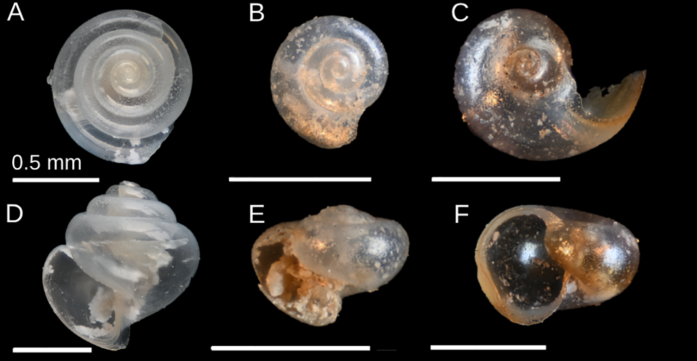
Photographs of species used in the study: Limacina retroversa(A, D), Limacina helicina pacifica(B, E), and Heliconoides inflatus(C, F). Shells are oriented apically (A-C) and aperturally (D-F). Scale bars represent 0.5 mm.
Pteropods and their responses to acidification have been extensively studied over the past two decades. These responses include changes in shell size (Lischka et al., 2011), shell surface dissolution (Lischka and Riebesell, 2012; Busch et al., 2014; Niemi et al., 2021), shell thickness (Mekkes et al., 2021a; Roger et al., 2012; Howes et al., 2017), metabolic rates (Lischka and Riebesell, 2017; Maas et al., 2018; Moya et al., 2016), respiration (Maas et al., 2018), and gene expression patterns (Moya et al., 2016). Shell responses are the most common metrics for acidification impacts because they can be assessed after organismal death and without preservation of genetic material. These responses are measured in a variety of ways. The most common method of evaluating dissolution in pteropods is a semi-quantitative SEM-based method that grades shell surface dissolution on a scale of 0 (pristine) to 3 (dissolution of the external shell layer and inner layers) and assigns a percent coverage of shell surface to each dissolution “type” (Bednaršek et al., 2012a). This method has been previously used to quantify dissolution at various stages of life (Niemi et al., 2021; Mitchell, 2019) and to characterize pteropod shell microstructure for future application in biomaterials research (Ramos-Silva et al., 2021). The Limacina Dissolution Index (LDX) is a light microscopy method that grades shell dissolution on a semi-quantitative scale from pristine (0) to highly dissolved (5) based on shell luster and transparency (Gerhardt et al., 2000; Gerhardt and Henrich, 2001). As described in these publications, at LDX 0, shells are transparent and lustrous. At LDX 1, shells are lustrous but cloudy. Luster is maintained at LDX 2, but shells are completely white and opaque. At LDX 3, shells begin to lose their luster and become totally lustreless by LDX 4 due to the complete loss of the upper shell layer, LDX 5 is characterized by opaque, white, totally lustreless shells, as in LDX 4, but also includes additional shell damage such as perforations. LDX was developed as a dissolution proxy to track aragonite preservation in sediment cores via fossil specimens (Gerhardt et al., 2000). It has also been used in the fossil record to document past variability in ocean carbonate concentration and supersaturated environments (Wall-Palmer et al., 2013; Hallenberger et al., 2022). Additionally, studies assessing dissolution on modern pteropods have utilized LDX and similar semi-quantitative scales (Lischka et al., 2011; Lischka and Riebesell, 2012; Manno et al., 2012; Maas et al., 2023). Alternatively, micro-computed tomography (micro-CT) imaging produces shell thickness and volume data and is one of the few ways to obtain fully quantitative data on the impact of acidification on pteropod shell thickness. Micro-CT has been used to generate time series’ of how shell thickness has decreased over time in response to increasingly acidic conditions (e.g., Howes et al., 2017; Mekkes et al., 2021a).
Significant progress has been made in understanding and measuring the diversity of pteropod responses to acidification. However, establishing best practices in utilizing these responses for ocean acidification monitoring is an ongoing process. For example, a systematic comparison of light microscopy, CT, and SEM methods has not been completed. Previous research that has employed more than one of these metrics often compared only two methods (ex., Lischka et al., 2011 compared dissolution in light microscopy and SEM), or used one method only for visualization. Additionally, light microscopy methods like LDX have been largely underutilized in previous research. This lack of comparative information can make deciding which method(s) to implement in a monitoring program challenging. Compared to LDX, SEM and micro-CT methods produce higher resolution data, but they are time-intensive, less accessible with respect to equipment availability, and potentially cost-prohibitive. To access an SEM, researchers must undergo training and either pay $50-$110 per hour at an imaging lab or invest in their own SEM, which can cost hundreds of thousands of dollars (Mitchell, 2019). CT work involves either similar fees or limited availability at institutions offering free CT services (see discussion in Oakes et al., 2020). In contrast, LDX assessment only requires a binocular microscope, a common component of biological and earth science labs that is familiar to researchers of all levels. If LDX can effectively evaluate dissolution, it would be an ideal addition or substitute in ocean acidification monitoring programs; it is fast, essentially free, and immediately implementable within most research labs.
This paper compares light microscopy, CT, and SEM methods for assessing dissolution across the same specimens of three pteropod species that are commonly used in ocean acidification studies. In particular, this research seeks to elucidate the relationships among the different dissolution assessment methods and to determine the comparable effectiveness of light microscopy relative to more time- and cost- intensive techniques. This work will inform acidification monitoring efforts in two primary ways: by comparing the various dissolution methods and by investigating how these methods may be applied across multiple species.
2 Methods
2.1 Species studied
Higher-level pteropod taxonomy is complicated due to the lack of distinguishing shell morphological characteristics across taxa and rate heterogeneity, leading to similar yet conflicting classifications (Klussmann-Kolb and Dinapoli, 2006; Corse et al., 2013). For example, the gastropod classification of Bouchet et al. (2017) lists the order Pteropoda as consisting of three suborders: Euthecosomata (shelled), Gymnosomata (non-shelled), and Psuedothecosomata (variable), while acknowledging that Burridge et al. (2017), using molecular markers, found that Thecosomata (mucus-web feeders; Gilmer, 1974; Lalli and Gilmer, 1989; Conley et al., 2018) and Gymnosomata (active predators; Lalli and Gilmer, 1989; Dadon and Chauvin, 1998) were orders, with the former containing the suborders Euthecosomata and Psuedothecosomata. Most recently, a comprehensive phylogenomic study that included fossil data found support for the traditional taxonomic classification of the order Pteropoda consisting of the suborders Thecosomata and Gymnosomata, in which the former contains the infraorders Euthecosomata and Psuedothecosomata (Peijnenburg et al., 2020). Within the Euthecosomata, the superfamily Limacinoidea was recovered as a monophyletic group containing the genera Limacina and Heliconoides (Peijnenburg et al., 2020), the genera studied here.
This project focuses on the Limacina helicina species complex Phipps, 1774, Limacina retroversa J. Fleming, 1823, and Heliconoides inflatus d’Orbigny, 1835. The L. helicina species complex is composed of two subspecies: L. helicina Phipps, 1774 and L. helcina pacifica Dall, 1871 (Hunt et al., 2010; Janssen et al., 2019). While many studies do not identify pteropods down to the subspecies level, the L. helicina specimens used in this study were taxonomically evaluated in 2019 by a pteropod specialist who identified all specimens as L. helicina pacifica (Janssen et al., 2019).
All three species included in this study are well researched with respect to ocean acidification. The L. helicina (Figures 1B, E) species complex is one of the most common taxa used in ocean acidification studies; documented negative responses to acidified conditions include reduced shell thickness and increased shell dissolution and degradation for both juvenile and adult stages (Bednaršek et al., 2017a; Lischka et al., 2011; Busch et al., 2014; Mekkes et al., 2021a). L. retroversa (Figures 1A, D) responses to ocean acidification include changes in metabolism, calcification, early development survivorship, and the expression of genes related to biomineralization, metabolism, and neural function (Thabet et al., 2015; Maas et al., 2018; Mekkes et al., 2021b). This species also displays compounding impacts from ocean acidification and nanoplastics in laboratory conditions (Manno et al., 2022). H. inflatus (Figures 1C, F) responses to acidification include downregulated genes associated with metabolism and upregulated genes associated with calcification (Moya et al., 2016).
2.2 Shell structure
Like other shelled mollusks, pteropods produce shells using a biomineralization process controlled by the mantle (e.g., Marin et al., 2012). This process produces a series of two to five superposed calcified shell layers (Marin et al., 2012) and an outermost organic layer known as the periostracum, which can provide protection against dissolution (Peck et al., 2016a; Miller et al., 2023). Each calcified shell layer is an organo-mineral biocomposite comprised of aragonite crystals arranged in varying microstructures and a 0.1-5% organic fraction (e.g., Checa, 2018). For L. helicina and L. retroversa, the crystal structure of the adult shell consists of an outer and inner prismatic layer and an internal crossed lamellar layer (Figures 2A–D; Ramos-Silva et al., 2021). A helicoidal crystal structure may also occur beneath the prismatic layer in the protoconch (the embryonic shell) of Limacina species (Glacon et al., 1994). For H. inflatus, a simple helicoidal internal layer (Figures 2E-H; Ramos-Silva et al., 2021) is bounded by an inner prismatic layer (Glacon et al., 1994) and an external granular prismatic layer. Externally located crossed lamellar structures may also be present (Ramos-Silva et al., 2021), but were not observed in this study. Differences in shell structures among the species in this study impact their relative vulnerability to ocean acidification. Cavolinid pteropods and H. inflatus have a helical shell microstructure that has been found to be more susceptible to dissolution than the cross-lamellar microstructure of other pteropods, such as Limacina (Bé and Gilmer, 1977; Wall-Palmer et al., 2013).
Figure 2
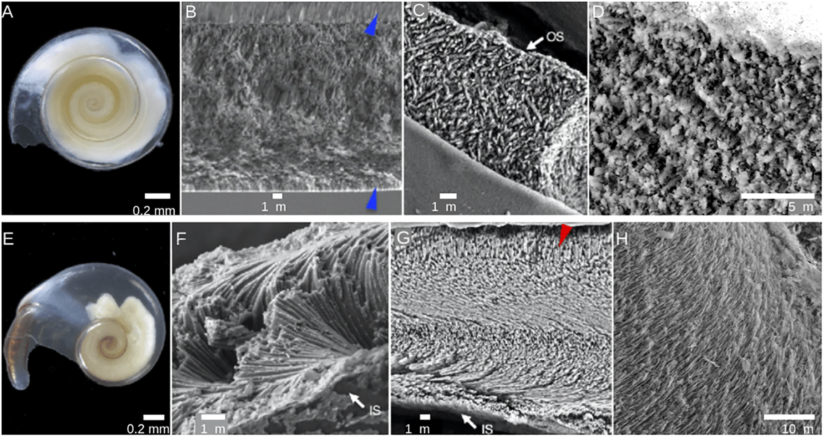
Light microscopy and SEM images of Limacina helicina(A–D) and Heliconoides inflatus(E–H). SEM images (B–D, F–H) demonstrate the differing shell structures between the two genera. Blue arrows indicate the prismatic layer. Images A–C, E, F–G are from Ramos-Silva et al., 2021, and have been adapted into this figure in compliance with its license (https://creativecommons.org/licenses/by/4.0/). (D,H) are original to this paper.
2.3 Specimen selection and handling
This study used 89 specimens from previous research and 56 newly studied specimens. Specimens missing more than approximately ¼ whorl were not used. The amount of missing whorl was determined by signs of breakage and remnant shell material where the outer whorl was fused to the inner whorl. Juvenile specimens were also excluded. Only specimens that were stored dry long term were used in this study to avoid post-mortem dissolution caused by storage in ethanol and other preservatives (following recommendations of Oakes et al., 2019a). Specimens were handled and manipulated using fine detail paintbrushes, modeling clay, and SEM tape, and never with tweezers or any metal instruments, to avoid damaging the shell. During shipments, specimens were packaged individually in microscope slide wells with pieces of nitrile gloves surrounding the specimens to reduce collisions with the glass slide cover and well walls.
Thirty L. helicina pacifica (hereafter L. helicina) specimens and 14 H. inflatus specimens were obtained on loan from the Natural History Museum of Los Angeles County (LACM) Malacology Collection. These specimens were collected at multiple localities from 1931–1981 within the California Current; detailed collection data are provided in the Supplementary Materials (Supplementary Table S1). Seasonal upwelling of cold subsurface water causes the California Current to be naturally prone to ocean acidification. In combination with biological processes like plankton blooms and sinking of organic matter, this produces trends in pH and aragonite saturation state that vary with depth, distance to shore, and time; pH can range from ~8.1 to ~7.7 due to these factors (Hauri et al., 2013 and references therein; Bednaršek et al., 2014 and references therein, Takeshita et al., 2021). pH was not measured during the cruises that collected the California Current specimens analyzed here. This poses no problem to the current study, since it compares how three dissolution metrics are interrelated, not how pteropods respond to pH or calcium carbonate saturation state.
Twenty-two H. inflatus specimens from Oakes and Sessa (2020) study of the Cariaco Basin were also included. The pH conditions of the Cariaco Basin vary from 7.57 to 8.04, depending on depth and latitude (Scranton et al., 2001) and waters remain saturated with respect to aragonite through the year (Oakes and Sessa, 2020). Due to the aragonite supersaturation, nutrient availability during periods of upwelling is the determining factor for shell strength and growth (Oakes and Sessa, 2020). These specimens were collected in 2013 and 2014 via a sediment trap deployed at a depth of 150 m. This trap collected specimens and debris falling in open water into one of 13 cups filled with borate-buffered formalin solution (described in Thunell et al., 2000). Each cup captured a 2-week interval of falling material, and the trap was collected and redeployed every six months as part of the CARIACO (Carbon Retention In A Colored Ocean) time series project (Thunell et al., 2000). The trap contents were washed, split, picked and stored as described in Thunell et al. (2000) and Tedesco and Thunell (2003). Pteropod specimens were picked from the washed and dried faunal samples in 2019 and were subjected to light microscopy and CT scanning as described in Oakes and Sessa (2020) and are reposited in the Academy of Natural Sciences of Philadelphia (ANSP) Malacology Collection (Supplementary Table S2).
Eight H. inflatus and two L. retroversa specimens from the Atlantis II cruise and two L. retroversa specimens from the H.M.S. Challenger expedition were borrowed from the Foraminifera collection of the Paleobiology Department of the Smithsonian National Museum of Natural History (NMNH). H.M.S. Challenger and Atlantis II specimens were collected using a plankton tow (Fox et al., 2020; Cifelli and McCloy, 1983). Due to the age and unspecified collection location of these specimens, pH conditions and aragonite saturation could not be specified.
Finally, sixty-seven L. retroversa specimens from St. Magnus Bay, Shetland Islands, UK were also assessed for this study. This region is rarely undersaturated, with an aragonite saturation ranging from 1.0 - 3.1 (Hartman et al., 2019). It has a surface pH that varies seasonally from 8.09 to 8.19 (Hartman et al., 2019), with the lower pH values generally seen during spring and summer (Bresnan et al., 2016; Findlay et al., 2022). The specimens were collected at 5 of 17 sampling stations on a transect running from the Olna Firth inlet to the open shelf in May through June of 2018 (see detailed description of sites in Dees, 2021). Specimens were collected via vertical plankton tows with a 125 µm-mesh bongo net (C. Angus, personal communication, May 16, 2018) deployed to maximum depths ranging from 107 to 145 meters (P. Dees, personal communication, June 4, 2020). The specimens were temporarily kept in 70% buffered ethanol during the cruise and shipping phases and were then picked and dried within 6 months of collection for long term storage to reduce any dissolution from the ethanol (i.e., Oakes et al., 2019a). All are reposited in the Academy of Natural Sciences of Philadelphia (ANSP) Invertebrate Paleontology Collection (Supplementary Table S2).
2.4 Light microscopy dissolution assessment
The LDX method utilizes the six preservation stages from Gerhardt et al. (2000), in which a score of 0 indicates a pristine shell and a score of 5 indicates severe corrosion (Figure 3). When examining pteropod specimens either through photographs or under a microscope, the following characteristics are taken into consideration for scoring: transparency, luster, and, in severely dissolved specimens, the removal of the entire surface layer and deeper layers (Gerhardt et al., 2000). As the specimens move up the LDX scale, transparency and luster decreases while (in more severe cases) exposure of inner shell layers increases.
Figure 3
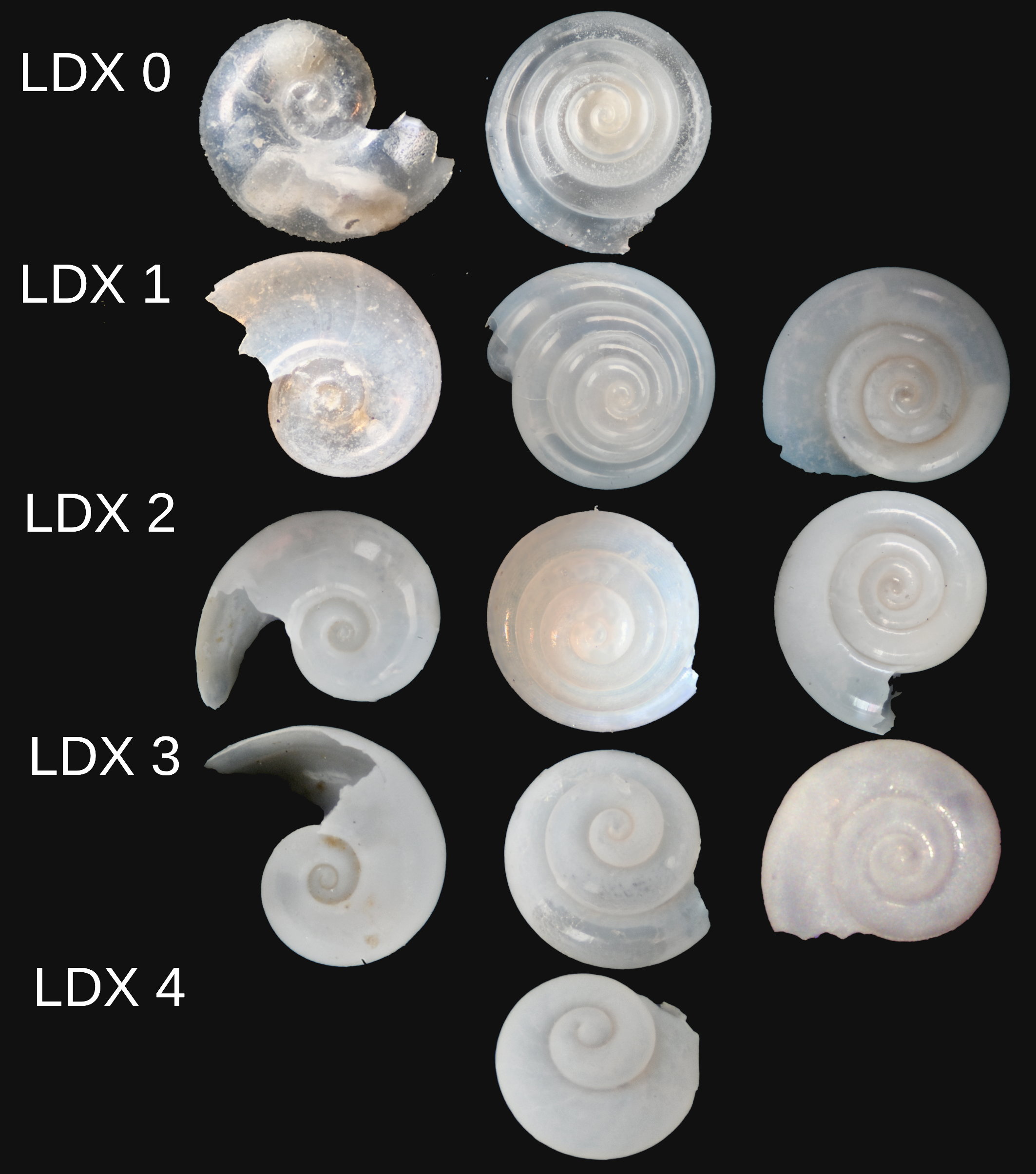
The Limacina Dissolution Index (LDX) from 0 (no dissolution) to 4 (highest dissolution of specimens observed in this study). Specimens on the left are Heliconoides inflatus, specimens in the middle column are Limacina retroversa, and specimens on the right are Limacina helicina. From LDX 0 to 2, specimen shells progress from transparent at LDX 0, to milky, and then to fully opaque and white at LDX 2. From LDX 2 to 4, shells progress from lustrous to no luster and no outer shell layer. Shells are not to scale.
Light microscopy was employed to photograph specimens using a standard photography rig containing a Nikon Z50 with two PK-13 auto extension tubes attached to a Bausch & Lomb monocular microscope, which produced higher resolution images relative to the Leica built-in camera on the monocular scope. This setup was then connected to a monitor that is operating Nikon Camera Control Pro (version 2.34.1, Nikon Inc., Tokyo, JPN; Camera Control Pro, 2021). Polarizers on the light source were used to minimize overexposure in photos due to the shiny nature of pteropod shells. Individual image slices were photographed manually using the microscope’s stage wheel and stacked in Helicon Focus 8 (version 8.2.2, Helicon Soft, Kharkiv, UA; Helicon Focus 8, 2022). LDX was then assessed based off these specimen images (Supplementary Plate 1). To determine whether LDX score is affected by using photographs versus when assessing via light microscope, Koester scored 105 shells both ways.
Taphonomic grading systems like the LDX are widely used across both paleontological and neontological disciplines, and studies emphasize the need for the training of new operators and of assessing inter-operator error (Kidwell, 2001; Rothfus, 2004). Several studies have found that greater inter-operator error is associated with less experienced operators (Rothfus, 2004; Soficaru et al., 2014; Wilczak et al., 2017; Ziegler and van Huet, 2021), and as such training new operators is essential to ensure reproducible results. Two of the co-authors, Koester and Mercado, had not previously worked with the LDX method. They were trained by first studying the LDX scale and images in Gerhardt and Henrich (2001) and other studies that employed the LDX method (Oakes et al., 2019a; Oakes and Sessa, 2020). They then practiced assigning scores and reviewed their scores with Oakes and Sessa, both of whom are experienced in assigning LDX scores. To assess whether there are differences in scores from different researchers, 142 shells were assessed by 2–4 authors (Supplementary Table S3).
2.5 Micro-computed tomography dissolution assessment
For most California Current specimens, CT scanning was conducted by lab technicians at the CT facilities at the University of Texas (UTCT) using a Zeiss Versa 620 scanner. Scans were run with a voltage of 80kV, a current of 10W, and an acquisition time ranging from 0.5-1.0 seconds. The resulting scan resolution from these parameters ranged from 0.7- to 2.2-micron voxels. The computer software programs Dragonfly (version 2022.1, ORS, Montreal, CAN; Dragonfly, 2022) and VG Studio Max (version 2023.2, Volume Graphics, Heidelberg, GER; VG Studio Max, 2023) were used to digitally remove non-shell materials, such as sediment or other organisms within or adhering to the shell and remnants of the pteropod body, from the resulting scan data and to measure shell width and height and calculate shell thickness. In Dragonfly, the Otsu method was utilized for density thresholding to separate the denser shell material from less-dense organic material and background air so that the shell could be isolated as a Region of Interest (ROI; Otsu, 1979). Some specimen scans required manual adjustments to the Otsu threshold to more accurately differentiate between shell and non-shell material. For the specimens processed with VG Studio Max, sediment and organic material were made into a ROI using the ‘Draw’ tool and then subsequently removed from the area of analysis (e.g., the shell) using the ROI ‘Rendering’ tool. With the non-shell ROI removed, a ‘surface determination’ was performed to select only the shell material for thickness analysis.
All Cariaco and Shetland specimens were CT scanned using the methods described in Oakes et al. (2020) and Oakes and Sessa (2020), at the American Museum of Natural History in New York, New York, or at General Electric Inspection Technologies in Lewistown, PA, with voxel resolution ranging from 1–2 microns. The Cariaco specimen CT data had been previously processed by Oakes and Sessa (2020) using VG Studio MAX. The Shetland CT data were processed using the same procedure described above for the California Current specimens.
For all specimens, shell thickness was determined in VG Studio Max, using the Sphere Method under Wall Thickness Analysis and then exporting the data from the Histogram tab. Bin sizes for histograms were set according to the specific specimen’s voxel size. Shell ROIs were converted into a masked version of the original scan and saved as a DICOM file for future reference and analysis. All scans are available for download on Morphosource under the project IDs: 000623860 (California Current Pteropod Scans Project), 00000C908 (Oakes and Sessa Pteropod Variability Project), and 000640972 (Academy of Natural Sciences Invertebrate Paleontology Collection Project).
2.6 Scanning electron microscopy dissolution assessment
SEM imaging was conducted by Koester at the Singh Laboratory at the University of Pennsylvania using a Quanta 600 FEG ESEM (Supplementary Plate 2). Specimens were kept in an unaltered state without sputter coating. Following the commonly employed pteropod dissolution method of Bednaršek et al. (2012a), Koester ranked dissolution from pristine (Type 0) to highly dissolved (Type 3) based on the amount of dissolution of the surface prismatic layer and the underlying shell layer (Figure 4). Dissolution is either reported as the maximum dissolution type observed throughout the entire shell (Bednaršek et al., 2014; Mitchell, 2019) or as a percentage of the surface area of each dissolution type (Bednaršek et al., 2012a; Mekkes et al., 2021a). Both evaluations were included in this study and were assessed when the specimen was oriented apically, as in Figure 3, and percentage of surface area was determined visually, in a manner similar to estimating mineral composition of a petrographic thin section. Chemical baths and plasma etching are still common practice for preparing specimens for SEM analysis. Following the recommendations of Peck et al., (2016a; 2016b), these methods were not employed here because they could remove the shells’ inter- and intra-crystalline organic matrix, thereby increasing the appearance of dissolution. Initial SEM scans indicated that the shell surface and any dissolution could be sufficiently observed without subjecting specimens to these methods.
Figure 4
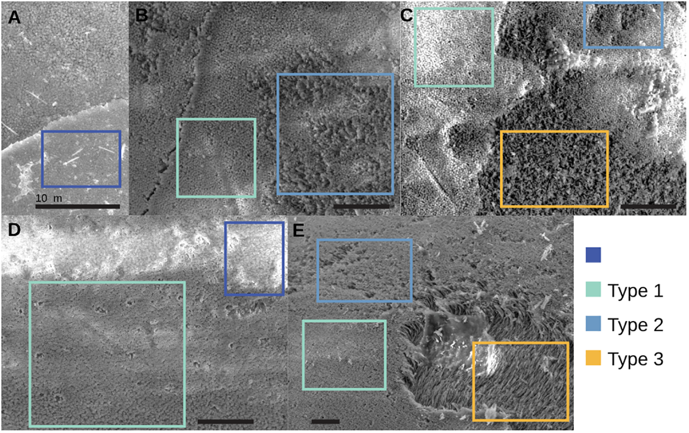
SEM images of Type 0 to 3 dissolution examples on Limacina helicina(A–C) and Heliconoides inflatus(D, E) specimens. All scale bars are 10 microns. Colored boxes highlight examples of the different dissolution types.
2.7 Specimen measurements
All specimens were measured to provide information on size. Height and width were taken from CT scans using the ‘Ruler Tool’ in Dragonfly. Height was measured along the shell columella, the axis around which the shell coils as it grows (Supplementary Figure S1). Width was measured perpendicular to the height measurement at the widest point of the specimen on the apertural plane, a plane aligned with the aperture of the shell that bisects the shell and columella (Supplementary Figure S1).
Whorl count is used as a proxy for gastropod specimen age (Kuznik-Kowalska, 2006; Schöne et al., 2007) and thus pteropod age. Under ambient oceanic conditions, pteropods will increase their entire shell size over time (Mekkes et al., 2021b), subsequently increasing their whorl count. Following the methods of Janssen (2007), whorls are counted when viewing the shell in an apical orientation. The first whorl begins at a visualized straight line that divides the semicircular nucleus of the protoconch (protoconch-1) from subsequent shell growth. Each full whorl is completed when a 360° rotation is made from the visualized line; total whorl count is estimated to the nearest 1/8 whorl when the aperture is reached (Supplementary Figure S1).
2.8 Statistical analysis
Because Oakes and Sessa (2020) found that larger shells of H. inflatus specimens from the Cariaco Basin were thicker, they used a simple linear regression model of shell thickness and width (referred to as diameter in their study) to remove the influence of size on thickness (Supplementary Text 1). These normalized thickness values were referred to as ‘residual thickness’. Here, Spearman correlation tests between shell thickness and width are used to determine if size influences thickness in the L. helicina, L. retroversa, and expanded H. inflatus datasets (Supplementary Table S4). For any species where a significant correlation was found, the ‘residual thickness’ of Oakes and Sessa (2020) is used instead of modal thickness.
The Spearman correlation test accounts for potential non-linear relationships between variables and therefore was used to test for significant relationships among all dissolution metrics (Supplementary Text 1). Eighteen correlation tests were conducted. A Bonferroni correction was applied to the resulting p-values (Bonferroni, 1936), adjusting the threshold of significance from 0.05 to 0.0028 to account for the increased risk of a Type I error, i.e., a spurious significant correlation due to the large number of correlations performed (Abdi, 2007). Any correlation that is highly significant (p < 0.001) before Bonferroni correction (p < 0.0028) will therefore remain significant after.
Using beta regression, locality and species were examined as potential influencing variables on the most common significant relationship from the Spearman correlation tests (Supplementary Text 2). Models were fit two ways, by maximum likelihood using the R-package ‘betareg’ (Cribari-Neto and Zeileis, 2010) and Bayesian simulation (Markov Chain Monte Carlo) using ‘brms’ (Bürkner, 2017). Fits from both methods were assessed using appropriate methods, inspecting plots of residuals for the maximum likelihood analysis and posterior predictive checks for the Bayesian analysis, respectively. For Bayesian fits, the R-package ‘loo’ was used, which performs a “leave one out” simulation of fits and predictions to estimate an expected log pointwise probability density (ELPD; Vehtari et al., 2024). For the maximum likelihood fits, the AIC method of model ranking was utilized. Raw AIC values are random and subject to sampling error.
3 Results
3.1 Data overview
Some shells were lost or destroyed during various stages of analysis and so were not analyzed using all three dissolution methods – 145 specimens were analyzed via light microscopy; 141 were CT scanned; and 134 were imaged with SEM. All dissolution assessments are listed by specimen in Supplementary Materials (Supplementary Table S2).
During SEM imaging, abnormal structures were observed on the surface of all studied specimens from the Atlantis II and Challenger expeditions (4 L. retroversa and 8 H. inflatus specimens). These structures, which ranged from superficial nodules to altered crystal structures of the shell layers, covered substantial portions of each specimen. These features do not fall within the SEM dissolution method and could alter LDX values and were therefore removed and not analyzed further. Additionally, one L. helicina specimen lot (LACM-1951-65.2) is from ~800 m, while all other specimens are from <200 m, creating a significantly different taphonomic history for this deep lot relative to the rest of the dataset. These deep lot specimens were very likely collected dead after falling through the water column for hundreds of meters. This would provide ample opportunity for the organic body’s decay to cause internal dissolution (as described in Oakes et al., 2019b), which would increase LDX values but not the dissolution measured by SEM on the external shell. This lot strongly diverged from negative relationship between LDX and SEM Type 0 displayed by all other specimens across the three species (Supplementary Figure S2), highlighting the importance of standardized collection and preservation techniques, and was therefore removed from analyses (see Table 1 for finalized specimen counts).
Table 1
| Species | Light Microscopy | CT | SEM |
|---|---|---|---|
| L. helicina | 13 | 10 | 13 |
| L. retroversa | 67 | 67 | 65 |
| H. inflatus | 36 | 36 | 34 |
| Total | 116 | 113 | 112 |
Number of specimens in each analysis by species.
Specimens that broke after only completing one of the three analyses and those that had unique taphonomic histories relative to the rest of the dataset have been removed.
LDX values in L. helicina specimens ranged from 0.5 - 3; H. inflatus values ranged from 0 - 3.5 (Table 2). L. retroversa had the largest range, from LDX 0 - 4. Modal shell thickness ranged from 5 - 10 μm, 3 - 13 μm, and 5 - 16 μm, for L. helicina, L. retroversa, and H. inflatus respectively. For SEM maximum type dissolution, L. helicina ranged from 0 - 3, L. retroversa ranged from 0 - 3, and H. inflatus ranged from 2 - 3. H. inflatus specimens had the largest amounts of Type 3 dissolution overall, while L. retroversa had an average Type 3 percent coverage of 0.6%.
Table 2
| LDX | L. helicina | L. retroversa | H. inflatus |
|---|---|---|---|
| 0 LDX | 0 | 15 | 3 |
| 0.5 LDX | 3 | 17 | 5 |
| 1 LDX | 1 | 13 | 6 |
| 1.5 LDX | 3 | 6 | 3 |
| 2 LDX | 4 | 2 | 10 |
| 2.5 LDX | 0 | 4 | 1 |
| 3 LDX | 2 | 8 | 7 |
| 3.5 LDX | 0 | 1 | 1 |
| 4 LDX | 0 | 1 | 0 |
Number of specimens in each LDX category by species.
Four researchers evaluated and assigned LDX values to specimens. These values were compared to evaluate how this metric varies by researcher, and the average absolute difference among LDX assignments was 0.27 units (Supplementary Table S3). The average difference between LDX assignments made using a light microscope versus viewing a specimen photograph was also small (0.35 LDX units; Supplementary Table S3). Luster and transparency did not change in lockstep for every specimen. Thus, specimens with the same score can have slightly different appearances regarding these characteristics, which could contribute to variability in LDX assignments.
3.2 Limacina helicina
When comparing the SEM type percent composition to the LDX of each specimen, there is a trend of decreasing pristine shell (Type 0) and increasing proportions of Type 1, 2, and 3 dissolution as LDX dissolution increases (Figure 5). A Spearman analysis shows that LDX is significantly correlated to SEM Type 0 (rho = -0.90, p < 0.001) both before and after Bonferroni correction (p < 0.05 to p < 0.0028; Supplementary Figure S3). SEM maximum dissolution was correlated to SEM Type 0 (rho = -0.59, p < 0.05) and LDX (rho = 0.59, p < 0.05), but only before the Bonferroni correction. Modal shell thickness was not correlated with shell width (rho = 0.52, p = 0.13), and therefore residual thickness was not used to replace the raw thickness values (Supplementary Table S4). Raw thickness was not significantly correlated to any other dissolution metric in the Spearman rho analysis.
Figure 5
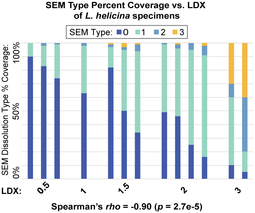
The percent coverage of the four SEM dissolution types for Limacina helicina specimens, organized by increasing LDX along the x-axis. Each bar represents a specimen.
3.3 Limacina retroversa
When comparing the SEM type percent composition of each specimen to LDX (Figure 6), a general trend of increasing proportions of Type 1–3 dissolution and decreasing proportions of pristine shell (Type 0) as LDX increases was again observed. The Spearman correlations among LDX and SEM metrics quantitatively support this finding (Supplementary Figure S4). Both before and after Bonferroni correction, LDX and percent shell coverage of SEM Type 0 were negatively correlated (rho = -0.88, p < 0.001) and LDX and SEM maximum dissolution type were positivity correlated (rho = 0.85, p < 0.001). Percent shell coverage of SEM Type 0 and SEM maximum dissolution type were also negatively correlated after Bonferroni correction (rho = -0.92, p < 0.001). Overall, these results indicate that increased dissolution as measured by LDX equates to increased dissolution as measured by the SEM type metrics. Within the L. retroversa dataset, CT modal shell thickness was not correlated to width (rho = -0.10, p = 0.41; Supplementary Table S4), and therefore residual thickness did not replace raw thickness in the Spearman rho analysis.
Figure 6
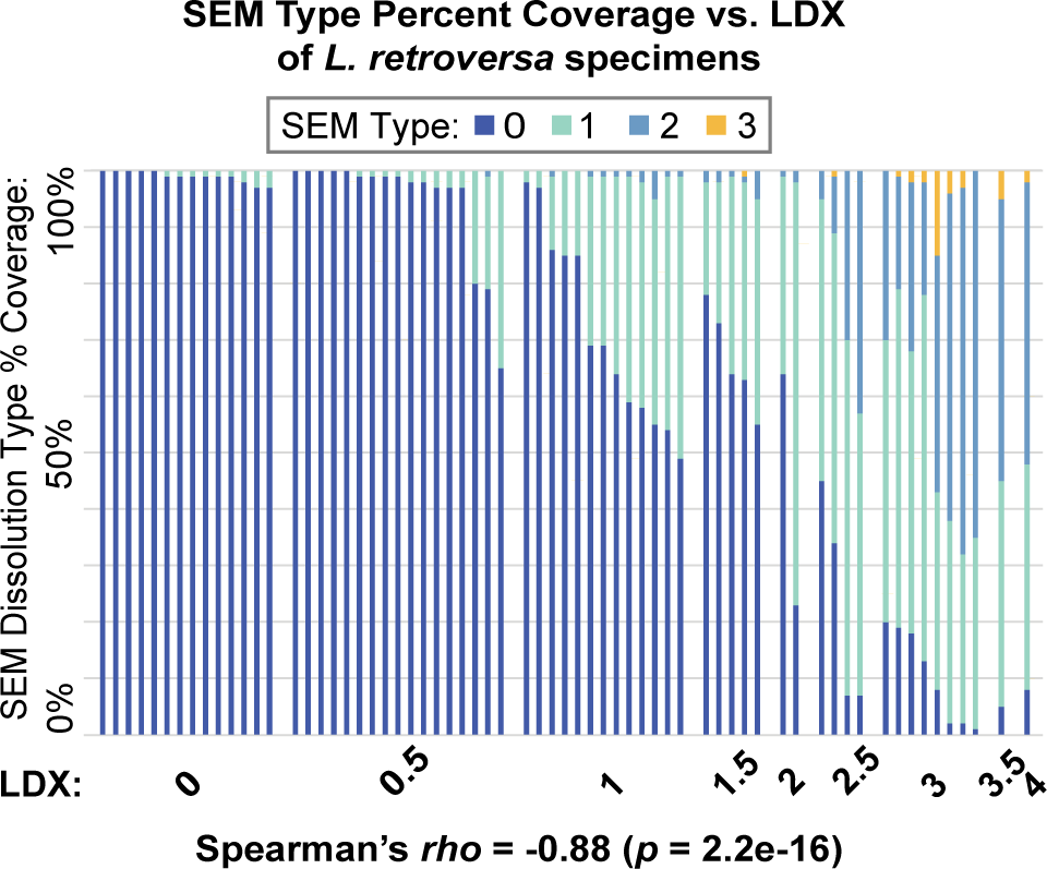
The percent coverage of the four SEM dissolution types for Limacina retroversa specimens, organized by increasing LDX along the x-axis. Each bar represents a specimen.
3.4 Heliconoides inflatus
When comparing the SEM type percent composition to the LDX of each H. inflatus specimen (Figure 7), proportions of Type 1–3 dissolution generally increase as LDX dissolution increases. Modal thickness was significantly correlated to shell diameter (rho = 0.38, p < 0.05) but not whorl count (rho = 0.09, p = 0.61; Supplementary Table S4). Due to this correlation, residual thickness replaced raw thickness in this dataset. Like L. retroversa, H. inflatus had a strong, significant, and negative correlation between LDX and percent coverage of pristine shell (SEM Type 0; rho = -0.84, p < 0.001; Supplementary Figure S5). LDX was also positively correlated to SEM maximum dissolution type (rho = 0.41, p < 0.05), but this correlation was not maintained after Bonferroni correction. Percent coverage of SEM Type 0 and SEM maximum dissolution type were also negatively correlated before and after Bonferroni correction (rho = -0.50, p < 0.01).
Figure 7
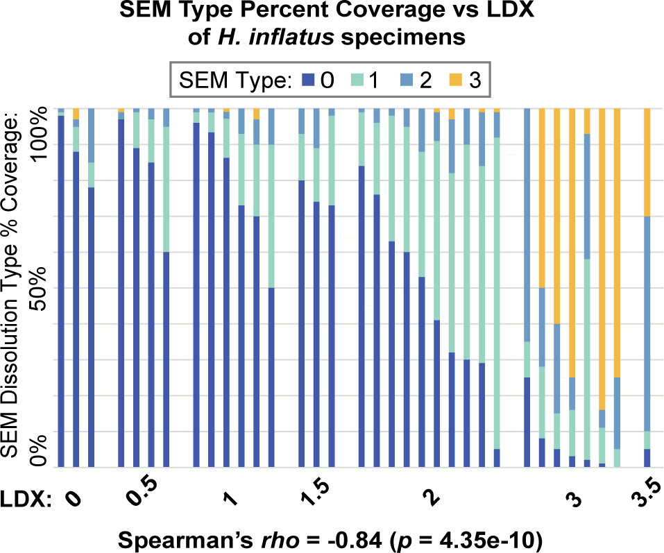
The percent coverage of the four SEM dissolution types for Heliconoides inflatus specimens, organized by increasing LDX along the x-axis. Each bar represents a specimen.
3.5 Comparison of SEM. dissolution variability vs. LDX across species and localities
A negative correlation between LDX and SEM Type 0 (pristine) percent shell coverage was the most common significant correlation among the three methods. To investigate the influence of species and locality on this relationship, a beta regression with a logit link function was used. Using both maximum likelihood estimation and Bayesian simulation, four models were considered: 1) a model with LDX and no other interactions, 2) a model with all three species separated, 3) a model with L. helicina and L. retroversa combined and H. inflatus separate (to assess influence of generic-level differences and their associated shell structure variations), and 4) a model with all three species separated and H. inflatus further divided by locality. Both maximum likelihood and Bayesian approaches produced the same ranking of the four models by accuracy of fit (Table 3). The maximum likelihood results indicate model 4 (Figure 8), where all species are distinct and H. inflatus is further divided by locality, is most supported, while the Bayesian results show models 4, 1, and 2 as equally plausible, since their ELPD difference is less than 4 (Sivula et al., 2020). Results for this analysis with lot LACM-1951-65.2 included can be found in the Supplementary Materials (Supplementary Table S5, Supplementary Figure S6). Other potential influences on the data, such as shell size and thickness, were assessed for influence in each species dataset, but did not appear to influence the relationship between LDX and SEM Type 0.
Table 3
| Analysis: | Max. Likelihood | Bayesian Simulation | ||
|---|---|---|---|---|
| Model | AIC | dAIC | ELPD_diff | se_diff |
| 4: SEM Type 0% ~ Species + LDX : Species + Locality | -281.868 | 0 | 0 | 0 |
| 1: SEM Type 0% ~ LDX | -276.683 | 5.185 | -2.926 | 3.409 |
| 2: SEM Type 0% ~ Species + LDX : Species | -275.657 | 6.211 | -3.334 | 2.799 |
| 3: SEM Type 0% ~ Species + LDX : Species (Limacina species combined) | -274.608 | 7.26 | -4.053 | 3.203 |
Maximum likelihood and Bayesian simulation beta regression results comparing various models. A ΔAIC > 2 or a ΔELPD > 4 between models is taken to be significant.
Figure 8
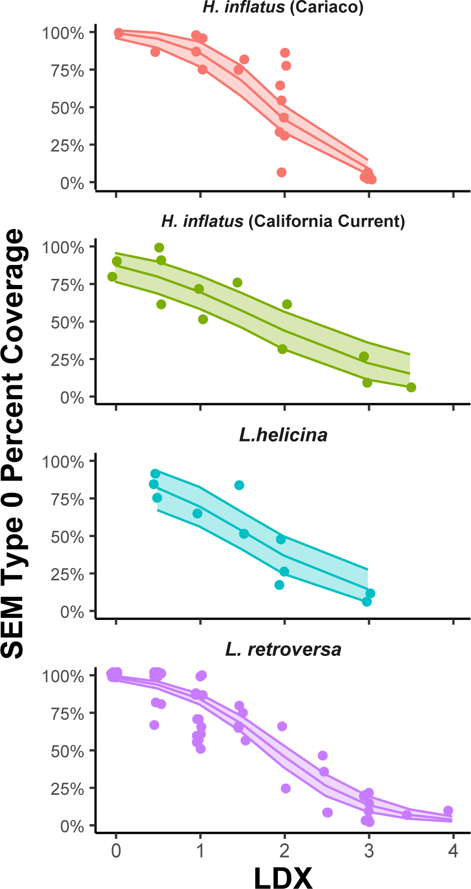
Model 4 of the relationship between SEM Type 0 percent coverage and LDX with a 95% confidence interval; all three species are separated and Helicina inflatus is also divided by locality.
3.6 Visual comparison of metrics
Light microscopy photos, SEM images, and CT heatmaps were compared side by side for a qualitative visual analysis (Figure 9; Supplementary Figure S7). SEM dissolution Type 3 was often visible in CT shell thickness heatmaps, but smaller patches of both Type 3 and 2 dissolution were often lost because of the lower resolution of the shape meshes that are used to produce the heatmaps (Figure 9). Patches of Type 3 dissolution were also often visible in light microscopy as gouges in the shell surface (Figures 9A; Supplementary Figure S8B). Additionally, differentiating between types of dissolution severity observed in SEM was often possible with light microscopy, when the patches of dissolution were large enough to be visible under the magnification of the light microscope (Supplementary Figure S8A).
Figure 9
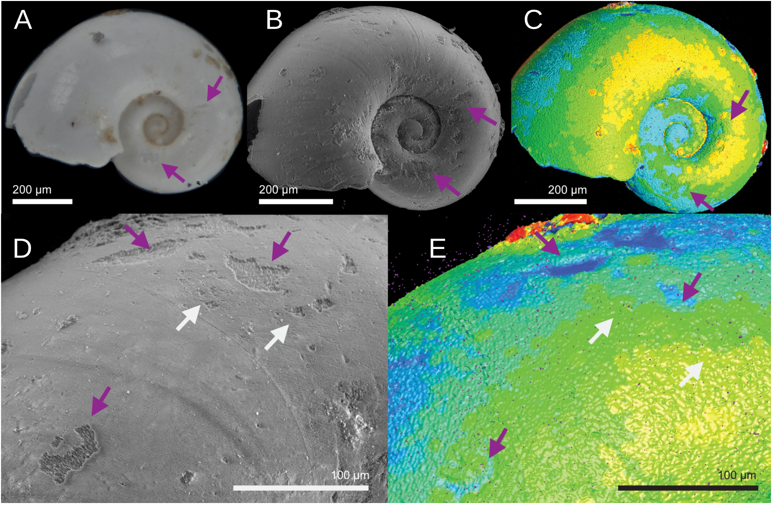
Comparison of a Heliconoides inflatus specimen (ANSP_477914_09) across light microscopy (A), SEM (B, D), and CT (C, E). In the CT thickness heatmaps, warmer colors equate to the thickest portions of the shell and cooler colors represent thinner areas. In the SEM images, purple arrows indicate examples of SEM type dissolution visible with other imaging methods and white arrows indicate patches of SEM type dissolution not visible with other imaging methods.
4 Discussion
4.1 Light microscopy LDX as a substitute for SEM metrics
Implementing LDX in ocean acidification studies requires minimal training and results in consistent scoring amongst researchers (Supplementary Table S3). Researchers new to this method will be able to become proficient within a day of reading and practice, provided that they can train with a researcher experienced in assigning LDX, since there are multiple criteria for dissolution. Additionally, LDX is significantly faster and cheaper than SEM based on the equipment time and costs for this study (Table 4).
Table 4
| Tool | Time per specimen | Cost per specimen |
|---|---|---|
| Light microscopy | 1-5 mins | free |
| SEM (max. vs. % coverage) | 5-30 mins/60 - 80 mins | ~$12/~$47 |
| CT | 35 mins scanning & 50 mins processing | $75 |
Time and cost per specimen for each tool of dissolution analysis, based on this study’s processing rates and equipment costs at UTCT and Singh Center for Nanotechnology.
SEM is divided into assessing only maximum dissolution type versus assessing percent coverage of each SEM dissolution type.
Among the five dissolution metrics, a negative relationship between LDX and SEM Type 0 percent coverage was the most common significant correlation, occurring in all three species. This relationship persists regardless of shell microstructure type (i.e., crossed lamellar vs. helical; see Section 1.3). Furthermore, these taxa were collected in locations with different oceanographic regimes, ranging from a relatively shallow subpolar bay (L. retroversa) to the tropical, aragonite-supersaturated Cariaco Basin (H. inflatus; Astor et al., 2013; Oakes et al., 2020) and the subtropical/temperate, aragonite-undersaturated California Current (H inflatus and L. helicina; Feely et al., 2016, 2008). Despite this wide variety of oceanographic conditions, the correlation between LDX and SEM Type 0 percent coverage was retained. This correlation is also maintained across a variety of collection and preservation methods. Even if this study removed collection and preservation as potentially confounding variables by only analyzing L. retroversa, a significant negative correlation between LDX and SEM Type 0 percent coverage is still demonstrated. This resilience of this result supports the hypothesis that the faster and less expensive LDX metric can perform as a substitute for SEM-based dissolution assessment. The authors suggest using a combination of LDX and SEM for analyzing shell dissolution—where LDX is used to assess the entirety of specimens and SEM is used on a minority of specimens determined by the time and resources available.
Further research is still merited to understand why some pteropod specimens do not show a relationship between LDX and SEM dissolution; perhaps the opacity method (Bergan et al., 2017), a light microscopy dissolution metric that quantitatively assesses changes in shell transparency, could provide additional insights.
4.2 Influence of location and species on LDX and SEM Type 0 relationship
Both types of beta regression showed that separating the dataset by species and locality produced the best model fits for the relationship between LDX and SEM Type 0. While these results are statistically significant, they may not be scientifically important, due to the inherent variability in both LDX and SEM type dissolution as semi-quantitative methods (i.e., Supplementary Figure S9), the differences in imaging resolution among the techniques, and the small number of specimens in many LDX categories. In particular, L. helicina and H. inflatus have small sample sizes when split by locality. Additionally, the L. helicina LDX dataset ranges from 0.5 to 3, with 14 of the 30 specimens scoring an LDX of 2, whereas the other species encompass a larger and more distributed range of LDX values (Table 2). Furthermore, the confidence regions of the different species in model 4 largely overlap with one another (Figure 8). While the California Current and the Cariaco Basin specimens of H. inflatus experienced different conditions, it is unclear how this could have led to the locations having different relationships between LDX and SEM Type 0. Therefore, we consider model 1, that of no species or locality, which is ranked as the second most plausible, to most accurately represent the relationship between LDX and SEM Type 0 based on the data currently available. Future studies should increase the sample size for all species, and particularly for L. helicina, across the LDX and SEM Type scales.
4.3 SEM maximum type dissolution as a potential substitute for SEM percent coverage metrics
SEM maximum dissolution may serve as a substitute for SEM Type 0 percent coverage, saving SEM lab time and usage fees. However, the significance of this correlation was only maintained after Bonferroni correction in L. retroversa, so this relationship needs additional data (in the form of increasing specimen numbers) and testing. In this study, a thorough evaluation of all SEM dissolution Type percent coverages, including that of SEM Type 0, took 60–80 minutes per specimen, while a max dissolution assessment would have likely taken ~5–30 minutes per specimen, since Type 2 and Type 3 are relatively easy and quick to identify (Table 4). Previous research (Mitchell, 2019) reported that SEM type surface area assessment only took 20 minutes per specimen, but Koester found that more time was required, both as a new SEM user and to detect early stages of Type 1 dissolution. Regardless, substituting SEM maximum type dissolution for Type 0 would save research time and costs if a strong relationship between the two SEM metrics is established.
4.4 CT is not sensitive to minor dissolution
Across all species, modal shell thickness was not correlated to any dissolution metric after Bonferroni’s correction. Modal shell thickness can be influenced by shell size and it was correlated to diameter in one of the three species (H. inflatus). Residual thickness, which accounts for the impact of shell size on shell thickness, did not produce any correlations with other dissolution metrics in this species. Either a different method of normalizing shell thickness was required, or whole-shell thickness was not significantly correlated to dissolution within the generally lower range of dissolution severity displayed by these specimens. It is likely that the surface dissolution caused by lived ocean conditions does not thin the shell enough to cause a significant change in modal thickness.
Unlike the shell-averaged thickness results, CT thickness heatmaps display patches of severe surface dissolution. At the scan resolution range achieved in this study (generally 1.2 microns), CT shell thickness heatmaps detected SEM Type 3 dissolution but lacked sensitivity to detect Type 1 SEM dissolution and smaller patches of Type 2 dissolution (Figure 9). Although heatmaps captured surface dissolution better than modal thickness, CT remains less sensitive than SEM to surface dissolution.
While CT may not be effective at capturing shell thinning caused by dissolution, it can detect shell thinning caused by reduced calcification across temporal and geographic acidification gradients. One study in the Mediterranean found that the shell thickness of Styliola subula significantly decreased from 1921 to 2012 as pH decreased ~0.1 units (Howes et al., 2017). Another study from the California Current showed that shell thickness declined as aragonite saturation decreased along an acidification gradient caused by regional upwelling (Mekkes et al., 2021a). This aligns with the use of CT in detecting reduced calcification in other mollusks (Wall-Palmer et al., 2021; Chatzinikolaou et al., 2017; Meng et al., 2018; Barclay et al., 2020), in foraminifera (Kinoshita et al., 2022), and hard corals (Fantazzini et al., 2015; Fordyce et al., 2020). Additionally, CT has been used to detect areas of repair in pteropod shells in response to various types of damage (Peck et al., 2018). Furthermore, CT analyses have been useful in modeling saturation states and dissolution rates to model benthic calcium carbonate preservation (Sulpis et al., 2022). Due to these findings, CT is recommended for assessing the loss of calcification in aragonite-oversaturated regions, where the primary response is likely to be a loss of calcification, as opposed to shell dissolution, which is more likely to occur in areas experiencing saturation and undersaturation.
5 Conclusion
As the first study to quantitatively compare LDX and SEM dissolution methods on modern pteropods, this study provides a promising indication that light microscopy methods can act as a viable substitute for the more cost- and time-intensive SEM-based techniques. Further work incorporating larger sample sizes than what was possible here may illuminate whether there are different responses by species and by locality. Results show that implementing LDX requires minimal training and results in consistent scoring amongst researchers. Furthermore, this study demonstrates that the relationship between LDX and SEM metrics persists across multiple species and oceanographic conditions, which strengthens its use on a global scale. CT, SEM, and light microscopy all have strengths and drawbacks; this study will hopefully help ocean acidification monitoring efforts that use shell dissolution as a bioindicator save time and money by understanding and strategically utilizing available resources. By determining how these metrics are related, detection of ocean acidification impacts via pteropod dissolution can become more efficient while still producing informative data. The more accessible monitoring practices are, the more we will be able to understand the impacts of ocean acidification at both the local and global scales. In turn, the more accessible the data from this research becomes, the easier it will be to formulate effective, inclusive policy.
Statements
Data availability statement
The original contributions presented in the study are included in the article/Supplementary Material. Further inquiries can be directed to the corresponding author/s.
Ethics statement
The manuscript presents research on animals that do not require ethical approval for their study.
Author contributions
BK: Conceptualization, Data curation, Formal analysis, Funding acquisition, Investigation, Methodology, Project administration, Validation, Visualization, Writing – original draft, Writing – review & editing. JH: Formal analysis, Methodology, Writing – review & editing, Writing – original draft. MM: Writing – original draft, Writing – review & editing, Formal analysis, Visualization. OG: Writing – review & editing, Formal analysis. RO: Data curation, Methodology, Resources, Writing – review & editing, Supervision. JS: Conceptualization, Methodology, Resources, Software, Supervision, Writing – review & editing, Project administration, Funding acquisition, Data curation.
Funding
The author(s) declare that financial support was received for the research and/or publication of this article. This research has been financially supported by the Lerner Grey Fund for Marine Research and the Western Society of Malacologists McLean Grant, which partially covered travel, specimen shipping, supply, and SEM machine-time costs, and by the Academy of Natural Sciences of Drexel University John J. & Anna H. Gallagher Fellowship.
Acknowledgments
We are deeply indebted to Lindsey T. Groves at the Natural History Museum of Los Angeles, Paul Dees at Scottish Association for Marine Science, Chevonne Angus at University of the Highlands and Islands, and Brian Huber for providing specimens that made this work possible. We are also incredibly grateful for Elizabeth Watson and Gary Rosenberg for their thoughtful comments on earlier drafts of this manuscript. Light microscopy imaging was completed with the invaluable assistance of Emily Owens and Alexis Srogota. CT scanning was conducted by Morgan Hill Chase at the American Museum of Natural History X-ray Computed Tomography Facility and by Jessica Maisano at the University of Texas High-Resolution X-ray Computed Tomography Facility with support from NSF (NSF EAR-1762458 and NSF MRI EAR-0959384) and NASA (80NSSC23K0199). Additionally, many thanks are owed to Edward Stanley at the Florida Museum of Natural History, for advice on CT analysis. SEM work was carried out at the Singh Center for Nanotechnology which is supported by the NSF National Nanotechnology Coordinated Infrastructure Program under grant NNCI-2025608. We would also like to acknowledge Paula Ramos-Silva, for usage with modification of their original figure, and Paul Roberts at the Academy of Natural Sciences Library, for assistance in archival research. We are grateful to editor D. Shallin Busch and reviewers Jinlin Liu and Silke Lischka for their thoughtful comments.
Conflict of interest
The authors declare that the research was conducted in the absence of any commercial or financial relationships that could be construed as a potential conflict of interest.
Publisher’s note
All claims expressed in this article are solely those of the authors and do not necessarily represent those of their affiliated organizations, or those of the publisher, the editors and the reviewers. Any product that may be evaluated in this article, or claim that may be made by its manufacturer, is not guaranteed or endorsed by the publisher.
Supplementary material
The Supplementary Material for this article can be found online at: https://www.frontiersin.org/articles/10.3389/fmars.2025.1473333/full#supplementary-material
References
1
Abdi H. (2007). Bonferroni and Šidák corrections for multiple comparisons. Encyclop. Measure. Stat3. Available online at: https://personal.utdallas.edu/~herve/Abdi-Bonferroni2007-pretty.pdf (Accessed May 9, 2025).
2
Armstrong J. L. Boldt J. L. Cross A. D. Moss J. H. Davis N. D. Myers K. W. et al . (2005). Distribution, size, and interannual, seasonal and diel food habits of northern Gulf of Alaska juvenile pink salmon, Oncorhynchus gorbuscha. Deep Sea Res. Part II: Top. Stud. Oceanog.52, 247–265. doi: 10.1016/j.dsr2.2004.09.019
3
Astor Y. M. Lorenzoni L. Thunell R. C. Varela R. Muller-Karger F. E. Troccoli L. et al . (2013). Interannual variability in sea surface temperature and fCO2 changes in the Cariaco Basin. Deep Sea Res. Part II: Top. Stud. Oceanog.93, 33–43. doi: 10.1016/j.dsr2.2013.01.002
4
Barclay K. M. Gingras M. K. Packer S. T. Leighton L. R. (2020). The role of gastropod shell composition and microstructure in resisting dissolution caused by ocean acidification. Marine Environ. Res.162, 105105. doi: 10.1016/j.marenvres.2020.105105
5
Bé A. W. H. Gilmer R. W. (1977). A zoogeographic and taxonomic review of euthecosomatous Pteropoda. Oceanic Micropaleontol.1, 733–808.
6
Bednaršek N. Feely R. A. Reum J. C. P. Peterson B. Menkel J. Alin S. R. et al . (2014). Limacina helicina shell dissolution as an indicator of declining habitat suitability owing to ocean acidification in the California Current Ecosystem. Proc. R. Soc. B: Biol. Sci.281. doi: 10.1098/rspb.2014.0123
7
Bednaršek N. Feely R. A. Tolimieri N. Hermann A. J. Siedlecki S. Waldbusser G. G. et al . (2017a). Exposure history determines pteropod vulnerability to ocean acidification along the US West Coast. Sci. Rep.7, 4526. doi: 10.1038/s41598-017-03934-z
8
Bednaršek N. Klinger T. Harvey C. J. Weisberg S. McCabe R. M. Feely R. A. et al . (2017b). New ocean, new needs: Application of pteropod shell dissolution as a biological indicator for marine resource management. Ecol. Indic.76, 240–244. doi: 10.1016/j.ecolind.2017.01.025
9
Bednaršek N. Možina J. Vogt M. O’Brien C. J. Tarling G. A. (2012b). The global distribution of pteropods and their contribution to carbonate and carbon biomass in the modern ocean. Earth Syst. Sci. Data4(1), 167–186. doi: 10.5194/essd-4-167-2012
10
Bednaršek N. Tarling G. A. Bakker D. C. E. Fielding S. Cohen A. Kuzirian A. et al . (2012a). Description and quantification of pteropod shell dissolution: a sensitive bioindicator of ocean acidification. Global Change Biol.18, 2378–2388. doi: 10.1111/j.1365-2486.2012.02668.x
11
Bergan A. J. Lawson G. L. Maas A. E. Wang Z. A. (2017). The effect of elevated carbon dioxide on the sinking and swimming of the shelled pteropod Limacina retroversa. ICES J. Marine Sci.74, 1893–1905. doi: 10.1093/icesjms/fsx008
12
Bonferroni C. (1936). Teoria statistica delle classi e calcolo delle probabilita Vol. 8 (Pubblicazioni del R Istituto Superiore di Scienze Economiche e Commericiali di Firenze), 3–62.
13
Bouchet P. Rocroi J.-P. Hausdorf B. Kaim A. Kano Y. Nützel A. et al . (2017). Revised classification, nomenclator and typification of gastropod and monoplacophoran families. Malacologia61, 1–526. doi: 10.4002/040.061.0201
14
Bresnan E. Cook K. Hindson J. Hughes S. Lacaze J. Walsham P. et al . (2016). The scottish coastal observatory 1997–2013: part 1—Executive summary. Scot. Marine Freshw. Sci.7, 1881–1881. doi: 10.7489/1881-1
15
Bürkner P.-C. (2017). brms: an R package for bayesian multilevel models using stan. J. Stat. Softw.80, 1–28. doi: 10.18637/jss.v080.i01
16
Burridge A. K. Hörnlein C. Janssen A. W. Hughes M. Bush S. L. Marlétaz F. et al . (2017). Time-calibrated molecular phylogeny of pteropods. PLoS One12, e0177325. doi: 10.1371/journal.pone.0177325
17
Busch D. S. Maher M. Thibodeau P. McElhany P. (2014). Shell condition and survival of Puget Sound pteropods are impaired by ocean acidification conditions. PLoS One9, e105884. doi: 10.1371/journal.pone.0105884
18
Camera Control Pro 2. (2021). Version 2.34.1 (Tokyo, Japan: Nikon Inc).
19
Chatzinikolaou E. Grigoriou P. Keklikoglou K. Faulwetter S. Papageorgiou N. (2017). The combined effects of reduced pH and elevated temperature on the shell density of two gastropod species measured using micro-CT imaging. ICES J. Marine Sci.74, 1135–1149. doi: 10.1093/icesjms/fsw219
20
Checa A. G. (2018). Physical and biological determinants of the fabrication of molluscan shell microstructures. Front. Marine Sci.5. doi: 10.3389/fmars.2018.00353
21
Ciais P. Sabine C. Bala G. Bopp L. Brovkin V. Canadell J. et al . (2013). “Carbon and other biogeochemical cycles,” in Climate change 2013: The Physical Science Basis. Contribution of Working Group I to the Fifth Assessment Report of the Intergovernmental Panel on Climate Change (Cambridge, United Kingdom and New York, NY, USA: Cambridge University Press), 465–570.
22
Cifelli R. L. McCloy C. (1983). Planktonic foraminifera and euthecosomatus pteropods in the surface waters of the North Atlantic. J. Foraminifer. Res.13, 91–107. doi: 10.2113/gsjfr.13.2.91
23
Conley K. R. Lombard F. Sutherland K. R. (2018). Mammoth grazers on the ocean’s minuteness: a review of selective feeding using mucous meshes. Proc. R. Soc. B: Biol. Sci.285, 20180056. doi: 10.1098/rspb.2018.0056
24
Corse E. Rampal J. Cuoc C. Pech N. Perez Y. Gilles A. (2013). Phylogenetic analysis of thecosomata blainville 1824 (Holoplanktonic opisthobranchia) using morphological and molecular data. PLoS One8, e59439. doi: 10.1371/journal.pone.0059439
25
Cribari-Neto F. Zeileis A. (2010). Beta regression in R. J. Stat. Softw.34, 1–124. doi: 10.18637/jss.v034.i02
26
Dadon J. R. Chauvin S. F. (1998). Distribution and abundance of gymnosomata (Gastropoda: opisthobranchia) in the southwest atlantic. J. Molluscan Stud.64, 345–354. doi: 10.1093/mollus/64.3.345
27
Dees P. (2021). Improving the predictability of harmful algal blooms around the Shetland Islands. (dissertation). (Inverness, Scotland: University of the Highlands and Islands).
28
Doney S. C. Balch W. M. Fabry V. J. Feely R. A. (2009a). Ocean acidification: a critical emerging problem for the ocean sciences. Oceanography22, 16–25. doi: 10.5670/oceanog.2009.93
29
Doney S. C. Fabry V. J. Feely R. A. Kleypas J. A. (2009b). Ocean acidification: the other CO2 problem. Annu. Rev. Marine Sci.1, 169–192. doi: 10.1146/annurev.marine.010908.163834
30
Dragonfly. (2022). Version 2022.1 for Windows (Montreal, Canada: Object Research Systems (ORS) Inc).
31
Fabry V. J. (2008). Marine calcifiers in a high-CO2 ocean. Science320, 1020–1022. doi: 10.1126/science.1157130
32
Fabry V. J. Deuser W. G. (1992). Seasonal changes in the isotopic compositions and sinking fluxes of euthecosomatous pteropod shells in the Sargasso Sea. Paleoceanography7, 195–213. doi: 10.1029/91PA03138
33
Fantazzini P. Mengoli S. Pasquini L. Bortolotti V. Brizi L. Mariani M. et al . (2015). Gains and losses of coral skeletal porosity changes with ocean acidification acclimation. Nat. Commun.6, 7785. doi: 10.1038/ncomms8785
34
Feely R. A. Alin S. R. Carter B. Bednaršek N. Hales B. Chan F. et al . (2016). Chemical and biological impacts of ocean acidification along the west coast of North America. Estuarine Coastal Shelf Sci.183, 260–270. doi: 10.1016/j.ecss.2016.08.043
35
Feely R. A. Sabine C. L. Hernandez-Ayon J. M. Ianson D. Hales B. (2008). Evidence for upwelling of corrosive “acidified” water onto the continental shelf. Science320, 1490–1492. doi: 10.1126/science.1155676
36
Feely R. A. Sabine C. L. Lee K. Berelson W. Kleypas J. A. Fabry V. J. (2004). Impact of anthropogenic CO2 on the CaCO3 system in the oceans. Science305 (5682), 362–368. doi: 10.1126/science.1097329
37
Findlay H. S. Artoli Y. Birchenough S. N. R. Hartman S. León P. Stiasny M. (2022). Ocean acidification around the UK and Ireland. MCCIP Sci. Rev.1–31. doi: 10.14465/2022.reu03.oac
38
Fordyce A. J. Knuefing L. Ainsworth T. D. Beeching L. Turner M. Leggat W. (2020). Understanding decay in marine calcifiers: micro-CT analysis of skeletal structures provides insight into the impacts of a changing climate in marine ecosystems. Methods Ecol. Evol.11, 1021–1041. doi: 10.1111/2041-210x.13439
39
Fox L. Stukins S. Hill T. Miller C. G. (2020). Quantifying the effect of anthropogenic climate change on calcifying plankton. Sci. Rep.10, 1620. doi: 10.1038/s41598-020-58501-w
40
Gaylord B. Rivest E. Hill T. Sanford E. Shukla P. Ninokawa A. et al . (2018). “Califonia mussels as bio-indicators of ocean acidification,” in California’s Fourth Climate Assessment (California, USA: California Natural Resources Agency).
41
Gerhardt S. Groth H. Rühlemann C. Henrich R. (2000). Aragonite preservation in late Quaternary sediment cores on the Brazilian Continental Slope: implications for intermediate water circulation. Int. J. Earth Sci.88, 607–618. doi: 10.1007/s005310050291
42
Gerhardt S. Henrich R. (2001). Shell preservation of Limacina inflata (Pteropoda) in surface sediments from the Central and South Atlantic Ocean: a new proxy to determine the aragonite saturation state of water masses. Deep Sea Res. Part I: Oceanog. Res. Papers48, 2051–2071. doi: 10.1016/S0967-0637(01)00005-X
43
Gilmer R. W. (1974). Some aspects of feeding in thecosomatous pteropod molluscs. J. Exp. Marine Biol. Ecol.15, 127–144. doi: 10.1016/0022-0981(74)90039-2
44
Gilmer R. W. Harbison G. R. (1986). Morphology and field behavior of pteropod molluscs: feeding methods in the families Cavoliniidae, Limacinidae and Peraclididae (Gastropoda: Thecosomata). Marine Biol.91, 47–57. doi: 10.1007/BF00397570
45
Glacon G. Rampal J. Gaspard D. Guillaumin D. Staerker T. S. (1994). “Thecosomata (pteropods) and their remains in late Quaternary deposits on the Bougainville Guyot and the central New Hebrides Island Arc,” in Proceedings of the Ocean Drilling Program Scientific Results, vol. 134. , 319–334.
46
Gruber N. Clement D. Carter B. R. Feely R. A. Van Heuven S. Hoppema M. et al . (2019). The oceanic sink for anthropogenic CO2 from 1994 to 2007. Science363, 1193–1199. doi: 10.1126/aau5153
47
Guinotte J. M. Fabry V. J. (2008). Ocean acidification and its potential effects on marine ecosystems. Ann. New York Acad. Sci.1134, 320–342. doi: 10.1196/annals.1439.013
48
Hallenberger M. Reuning L. Takayanagi H. Iryu Y. Keul N. Ishiwa T. et al . (2022). The pteropod species Heliconoides inflatus as an archive of late Pleistocene to Holocene environmental conditions on the Northwest Shelf of Australia. Prog. Earth Planet. Sci.9, 49. doi: 10.1186/s40645-022-00507-1
49
Hartman S. E. Humphreys M. P. Kivimäe C. Woodward E. M. S. Kitidis V. McGrath T. et al . (2019). Seasonality and spatial heterogeneity of the surface ocean carbonate system in the northwest European continental shelf. Prog. oceanog.177, 101909. doi: 10.1016/j.pocean.2018.02.005
50
Hauri C. Gruber N. Vogt M. Doney S. C. Feely R. A. Lachkar Z. et al . (2013). Spatiotemporal variability and long-term trends of ocean acidification in the California Current System. Biogeosciences10, 193–216. doi: 10.5194/bg-10-193-2013
51
Helicon Focus 8. (2022). Version 8.2.2 (Kharkiv, Ukraine: Helicon Soft).
52
Howes E. L. Eagle R. A. Gattuso J.-P. Bijma J. (2017). Comparison of mediterranean pteropod shell biometrics and ultrastructure from historical, (1910 and 1921) and Present Day, (2012) samples provides baseline for monitoring effects of global change. PLoS One12, e0167891. doi: 10.1371/journal.pone.0167891
53
Hunt B. P. V. Pakhomov E. A. Hosie G. W. Siegel V. Ward P. Bernard K. (2008). Pteropods in southern ocean ecosystems. Prog. Oceanog.78, 193–221. doi: 10.1016/j.pocean.2008.06.001
54
Hunt B. Strugnell J. Bednarsek N. Linse K. Nelson R. J. Pakhomov E. et al . (2010). Poles apart: the “Bipolar” Pteropod species limacina helicina is genetically distinct between the arctic and antarctic oceans. PLoS One5, e9835. doi: 10.1371/journal.pone.0009835
55
Janssen A. W. (2007). Holoplanktonic mollusca (Gastropoda: pterotracheoidea, janthinoidea, thecosomata and gymnosomata) from the pliocene of pangasinan (Luzon, Philippines). Scripta Geol.135, 29–177. Available online at: https://repository.naturalis.nl/pub/314194 (Accessed May 9, 2025).
56
Janssen A. W. Bush S. L. Bednaršek N. (2019). The shelled pteropods of the northeast Pacific Ocean (Mollusca: Heterobranchia, Pteropoda). Zoosymposia13, 305–346. doi: 10.11646/ZOOSYMPOSIA.13.1.22
57
Juranek L. W. Russell A. D. Spero H. J. (2003). Seasonal oxygen and carbon isotope variability in euthecosomatous pteropods from the Sargasso Sea. Deep Sea Res. Part I: Oceanog. Res. Papers50, 231–245. doi: 10.1016/S0967-0637(02)00164-4
58
Keul N. Peijnenburg K. T. C. A. Andersen N. Kitidis V. Goetze E. Schneider R. R. (2017). Pteropods are excellent recorders of surface temperature and carbonate ion concentration. Sci. Rep.7, 12645. doi: 10.1038/s41598-017-11708-w
59
Kidwell S. M. (2001). Preservation of species abundance in marine death assemblages. Science294, 1091–1094. doi: 10.1126/science.1064539
60
Kinoshita S. Wang Q. Kuroyanagi A. Murayama M. Ujiié Y. Kawahata H. (2022). Response of planktic foraminiferal shells to ocean acidification and global warming assessed using micro-X-ray computed tomography. Paleontol. Res.26, 390–404. doi: 10.2517/PR200043
61
Klussmann-Kolb A. Dinapoli A. (2006). Systematic position of the pelagic Thecosomata and Gymnosomata within Opisthobranchia (Mollusca, Gastropoda) – revival of the Pteropoda. J. Zool. Syst. Evol. Res.44, 118–129. doi: 10.1111/j.1439-0469.2006.00351.x
62
Kuznik-Kowalska E. (2006). Age structure and growth rate of Aegopinella epipedostoma (Fagot 1879) (Gastropoda: pulmonata: zonitidae). Folia Malacol.14 (2), 71–74. doi: 10.12657/folmal.014.011
63
Lalli C. M. Gilmer R. W. (1989). “The thecosomes. Shelled pteropods,” in Pelagic snails. The biology of holoplanktonic gastropod molluscs. Eds. LalliC. M.GilmerR. W. (Stanford University Press, California).
64
Le Quéré C. Raupach M. R. Canadell J. G. Marland G. Bopp L. Ciais P. et al . (2009). Trends in the sources and sinks of carbon dioxide. Nat. Geosci.2, 831–836. doi: 10.1038/ngeo689
65
Lischka S. Büdenbender J. Boxhammer T. Riebesell U. (2011). Impact of ocean acidification and elevated temperatures on early juveniles of the polar shelled pteropod Limacina helicina mortality, shell degradation, and shell growth. Biogeosciences8, 919–932. doi: 10.5194/bg-8-919-2011
66
Lischka S. Riebesell U. (2012). Synergistic effects of ocean acidification and warming on overwintering pteropods in the Arctic. Global Change Biol.18, 3517–3528. doi: 10.1111/gcb.12020
67
Lischka S. Riebesell U. (2017). Metabolic response of Arctic pteropods to ocean acidification and warming during the polar night/twilight phase in Kongsfjord (Spitsbergen). Polar Biol.40, 1211–1227. doi: 10.1007/s00300-016-2044-5
68
Maas A. E. Lawson G. L. Bergan A. J. Tarrant A. M. (2018). Exposure to CO2 influences metabolism, calcification and gene expression of the thecosome pteropod Limacina retroversa. J. Exp. Biol.221, jeb164400. doi: 10.1242/jeb.164400
69
Maas A. E. Lawson G. L. Bergan A. J. Wang Z. A. Tarrant A. M. (2023). Sea butterflies in a pickle: Reliable biomarkers and seasonal sensitivity of pteropods to ocean acidification in the Gulf of Maine. bioRxiv. doi: 10.1101/2023.07.31.551235
70
Manno C. Morata N. Primicerio R. (2012). Limacina retroversa's response to combined effects of ocean acidification and sea water freshening. Estuarine, Coastal and Shelf Sci.113, 163–171. doi: 10.1016/j.ecss.2012.07.019
71
Manno C. Peck V. L. Corsi I. Bergami E. (2022). Under pressure: Nanoplastics as a further stressor for sub-Antarctic pteropods already tackling ocean acidification. Marine Pollut. Bull.174, 113176. doi: 10.1016/j.marpolbul.2021.113176
72
Marin F. Le Roy N. Marie B. (2012). The formation and mineralization of mollusk shell. Front. Bioscience-Scholar4, 1099–1125. doi: 10.2741/s321
73
Marshall D. J. Abdelhady A. A. Wah D. T. T. Mustapha N. Gödeke S. H. De Silva L. C. et al . (2019). Biomonitoring acidification using marine gastropods. Sci. Total Environ.692, 833–843. doi: 10.1016/j.scitotenv.2019.07.041
74
Mekkes L. Renema W. Bednaršek N. Alin S. R. Feely R. A. Huisman J. et al . (2021a). Pteropods make thinner shells in the upwelling region of the California Current Ecosystem. Sci. Rep.11, 1731. doi: 10.1038/s41598-021-81131-9
75
Mekkes L. Sepúlveda-Rodríguez G. Bielkinaitė G. Wall-Palmer D. Brummer G.-J. A. Dämmer L. K. et al . (2021b). Effects of ocean acidification on calcification of the sub-antarctic pteropod limacina retroversa. Front. Marine Sci.8. doi: 10.3389/fmars.2021.581432
76
Meng Y. Guo Z. Fitzer S. C. Upadhyay A. Chan V. B. Li C. et al . (2018). Ocean acidification reduces hardness and stiffness of the Portuguese oyster shell with impaired microstructure: a hierarchical analysis. Biogeosciences15, 6833–6846. doi: 10.5194/bg-15-6833-2018
77
Miller M. R. Oakes R. L. Covert P. A. Ianson D. Dower J. F. (2023). Evidence for an effective defence against ocean acidification in the key bioindicator pteropod Limacina helicina. ICES J. Marine Sci.80, 1329–1341. doi: 10.1093/icesjms/fsad059
78
Mitchell S. A. (2019). New Methods for Imaging and Quantifying Dissolution of Pteropods to Monitor the Impacts of Ocean Acidification (Ithaca, NY: Cornell University).
79
Moya A. Howes E. L. Lacoue-Labarthe T. Forêt S. Hanna B. Medina M. et al . (2016). Near-future pH conditions severely impact calcification, metabolism and the nervous system in the pteropod Heliconoides inflatus. Global Change Biol.22, 3888–3900. doi: 10.1111/gcb.13350
80
Mucci A. (1983). The solubility of calcite and aragonite in seawater at various salinities, temperatures, and one atmosphere total pressure. Am. J. Sci.283, 780–799. doi: 10.2475/ajs.283.7.780
81
Niemi A. Bednaršek N. Michel C. Feely R. A. Williams W. Azetsu-Scott K. et al . (2021). Biological impact of ocean acidification in the Canadian Arctic: Widespread severe pteropod shell dissolution in Amundsen Gulf. Front. Marine Sci.8. doi: 10.3389/fmars.2021.600184
82
Oakes R. L. Chase M. H. Siddall M. E. Sessa J. A. (2020). Testing the impact of two key scan parameters on the quality and repeatability of measurements from CT scan data. Palaeontol. Electron.23, 1. doi: 10.26879/942
83
Oakes R. L. Davis C. V. Sessa J. A. (2021). Using the stable isotopic composition of Heliconoides inflatus pteropod shells to determine calcification depth in the Cariaco Basin. Front. Marine Sci.7. doi: 10.3389/fmars.2020.553104
84
Oakes R. L. Peck V. L. Manno C. Bralower T. J. (2019a). Impact of preservation techniques on pteropod shell condition. Polar Biol.42, 257–269. doi: 10.1007/s00300-018-2419-x
85
Oakes R. L. Peck V. L. Manno C. Bralower T. J. (2019b). Degradation of internal organic matter is the main control on pteropod shell dissolution after death. Global Biogeochem. Cycles33, 749–760. doi: 10.1029/2019GB006223
86
Oakes R. L. Sessa J. A. (2020). Determining how biotic and abiotic variables affect the shell condition and parameters of Heliconoides inflatus pteropods from a sediment trap in the Cariaco Basin. Biogeosciences17, 1975–1990. doi: 10.5194/bg-17-1975-2020
87
Orr J. C. (2011). “Recent and future changes in ocean carbonate chemistry,” in Ocean acidification, vol. 1. (Oxford University Press, New York, United States), 41–66.
88
Orr J. C. Fabry V. J. Aumont O. Bopp L. Doney S. C. Feely R. A. et al . (2005). Anthropogenic ocean acidification over the twenty-first century and its impact on calcifying organisms. Nature437, 681–686. doi: 10.1038/nature04095
89
Otsu N. (1979). A threshold selection method from gray-level histograms. IEEE Trans. syst. man cybernetics9, 62–66. doi: 10.1109/TSMC.1979.4310076
90
Peck V. L. Oakes R. L. Harper E. M. Manno C. Tarling G. A. (2018). Pteropods counter mechanical damage and dissolution through extensive shell repair. Nat. Commun.9, 264. doi: 10.1038/s41467-017-02692-w
91
Peck V. L. Tarling G. A. Manno C. Harper E. M. (2016b). Response to comment “Vulnerability of pteropod (Limacina helicina) to ocean acidification: Shell dissolution occurs despite an intact organic layer” by Bednaršek et al. Deep Sea Res. Part II: Top. Stud. Oceanog.127, 57–59. doi: 10.1016/j.dsr2.2016.03.007
92
Peck V. L. Tarling G. A. Manno C. Harper E. M. Tynan E. (2016a). Outer organic layer and internal repair mechanism protects pteropod Limacina helicina from ocean acidification. Deep Sea Res. Part II: Top. Stud. Oceanog.127, 41–52. doi: 10.1016/j.dsr2.2015.12.005
93
Peijnenburg K. T. C. A. Janssen A. W. Wall-Palmer D. Goetze E. Maas A. E. Todd J. A. et al . (2020). The origin and diversification of pteropods precede past perturbations in the Earth’s carbon cycle. Proc. Natl. Acad. Sci.117, 25609–25617. doi: 10.1073/pnas.1920918117
94
Ramos-Silva P. Wall-Palmer D. Marlétaz F. Marin F. Peijnenburg K. T. C. A. (2022). Evolution and biomineralization of pteropod shells. J. Struct. Biol.213, 107779. doi: 10.1016/j.jsb.2021.107779
95
Ries J. B. Cohen A. L. McCorkle D. C. (2009). Marine calcifiers exhibit mixed responses to CO2-induced ocean acidification. Geology37, 1131–1134. doi: 10.1130/g30210a.1
96
Roger L. M. Richardson A. J. McKinnon A. D. Knott B. Matear R. Scadding C. (2012). Comparison of the shell structure of two tropical Thecosomata (Creseis acicula and Diacavolinia longirostris) from 1963 to 2009: potential implications for declining aragonite saturation. ICES J. Marine Sci.69(3), 465–474. doi: 10.1093/icesjms/fsr171
97
Rothfus T. A. (2004). “A new system for the classification of preservational quality of fossil assemblages,” In: GSA Annual Meeting (Denver, Colorado (USA): Denver).
98
Sabine C. L. Feely R. A. Gruber N. Key R. M. Lee K. Bullister J. L. et al . (2004). The oceanic sink for anthropogenic CO2. Science305, 367–371. doi: 10.1126/science.1097403
99
Schöne B. R. Rodland D. L. Wehrmann A. Heidel B. Oschmann W. Zhang Z. et al . (2007). Combined sclerochronologic and oxygen isotope analysis of gastropod shells (Gibbula cineraria, North Sea): life-history traits and utility as a high-resolution environmental archive for kelp forests. Marine Biol.150, 1237–1252. doi: 10.1007/s00227-006-0435-9
100
Scranton M. Taylor G. Varela R. Astor Y. Muller-Karger F. Lorenzoni L. et al . (2001). “CARIACO Ocean Time-Series data collected in the Cariaco Basin since 1995,” in Water temperature, salinity, dissolved oxygen and other parameters from Niskin-bottle water samples from research vessel Hermano Gines in the Cariaco Basin from 1995-11–8 through 2017-1-12 (NOAA National Centers for Environmental Information). Available at: https://www.ncei.noaa.gov/archive/accession/0201747. Dataset.
101
Shinn E. A. (2008). Corals as bioindicators of climate change. Environmental Bioindicators3(3-4), 149–152. doi: 10.48550/arXiv.2008.10296
102
Sivula T. M. Mans Matamoros, Asael A. Vehtari A. (2020). Uncertainty in bayesian leave-one-out cross-validation based model comparison. arXiv, 10296. doi: 10.48550/arXiv.2008.10296
103
Soficaru A. D. Constantinescu M. Culea M. Ionică C. (2014). Evaluation of discriminant functions for sexing skulls from visually assessed traits applied in the Rainer Osteological Collection (Bucharest, Romania). HOMO65, 464–475. doi: 10.1016/j.jchb.2014.08.004
104
Sulpis O. Priyanka A. Wolthers M. Munhoven G. Walker M. Middelburg J. J. (2022). Aragonite dissolution protects calcite at the seafloor. Nat. Commun.13. doi: 10.1038/s41467-022-28711-z
105
Takeshita Y. Jones B. D. Johnson K. S. Chavez F. P. Rudnick D. L. Blum M. et al . (2021). Accurate pH and O2 measurements from spray underwater gliders. J. Atmosph. Oceanic Technol.38, 181–195. doi: 10.1175/JTECH-D-20-0095.1
106
Tedesco K. A. Thunell R. C. (2003). Seasonal and interannual variations in planktonic foraminiferal flux and assemblage composition in the Cariaco Basin, Venezuela. J. Foraminifer. Res.33, 192–210. doi: 10.2113/33.3.192
107
Thabet A. A. Maas A. E. Lawson G. L. Tarrant A. M. (2015). Life cycle and early development of the thecosomatous pteropod Limacina retroversa in the Gulf of Maine, including the effect of elevated CO 2 levels. Marine Biol.162, 2235–2249. doi: 10.1007/s00227-015-2754-1
108
Thunell R. C. Varela R. Llano M. Collister J. Muller-Karger F. Bohrer R. (2000). Organic carbon fluxes, degradation, and accumulation in an anoxic basin: sediment trap results from the Cariaco Basin. Limnol. Oceanog.45, 300–308. doi: 10.4319/lo.2000.45.2.0300
109
Vehtari A. Gabry J. Magnusson M. Yao Y. Bürkner P. Paananen T. et al . (2024). “loo: Efficient leave-one-out cross-validation and WAIC for Bayesian models,” in R package version 2.8.0. Available at: https://mc-stan.org/loo/ (Accessed June 17, 2024).
110
VG Studio Max. (2023). Version 2023.2 (Heidelberg, Germany: Volume Graphics).
111
Wall-Palmer D. Mekkes L. Ramos-Silva P. Dämmer L. K. Goetze E. Bakker K. (2021). The impacts of past, present and future ocean chemistry on predatory planktonic snails. Royal Society of Open Sci.8 (8), 202265. doi: 10.1098/rsos.202265
112
Wall-Palmer D. Smart C. W. Hart M. B. (2013). In-life pteropod shell dissolution as an indicator of past ocean carbonate saturation. Quater. Sci. Rev.81, 29–34. doi: 10.1016/j.quascirev.2013.09.019
113
Whitfield M. (1975). The effect of increases in the atmospheric carbon dioxide content on the carbonate ion concentration of surface ocean water at 25°C. Limnol. Oceanog.20, 103–108. doi: 10.4319/lo.1975.20.1.0103
114
Widdicombe S. Isensee K. Artioli Y. Gaitán-Espitia J. D. Hauri C. Newton J. A. et al . (2023). Unifying biological field observations to detect and compare ocean acidification impacts across marine species and ecosystems: what to monitor and why. Ocean Sci.19, 101–119. doi: 10.5194/os-19-101-2023
115
Wilczak C. A. Mariotti V. Pany-Kucera D. Villotte S. Henderson C. Y. (2017). Training and interobserver reliability in qualitative scoring of skeletal samples. J. Archaeol. Sci.: Rep.11, 69–79. doi: 10.1016/j.jasrep.2016.11.033
116
Zeebe R. E. (2012). History of seawater carbonate chemistry, atmospheric CO2, and ocean acidification. Annu. Rev. Earth Planet. Sci.40, 141–165. doi: 10.1146/annurev-earth-042711-105521
117
Ziegler T. van Huet S. (2021). Testing the reliability of the Fiorillo bone surface abrasion scale. J. Archaeol. Sci.: Rep.36, 102865. doi: 10.1016/j.jasrep.2021.102865
Summary
Keywords
pteropod, limacina, ocean acidification, shell dissolution, climate change, scanning electron microscopy, light microscopy, micro-computed tomography
Citation
Koester BE, Handley JC, Mercado M, Goodchild OA, Oakes RL and Sessa JA (2025) Assessing pteropod shell dissolution to advance ocean monitoring techniques: a methods comparison of SEM, CT, and light microscopy. Front. Mar. Sci. 12:1473333. doi: 10.3389/fmars.2025.1473333
Received
30 July 2024
Accepted
24 April 2025
Published
03 June 2025
Volume
12 - 2025
Edited by
D. Shallin Busch, National Oceanic and Atmospheric Administration (NOAA), United States
Reviewed by
Jinlin Liu, Tongji University, China
Silke Lischka, Association of German Research Centres (HZ), Germany
Updates
Copyright
© 2025 Koester, Handley, Mercado, Goodchild, Oakes and Sessa.
This is an open-access article distributed under the terms of the Creative Commons Attribution License (CC BY). The use, distribution or reproduction in other forums is permitted, provided the original author(s) and the copyright owner(s) are credited and that the original publication in this journal is cited, in accordance with accepted academic practice. No use, distribution or reproduction is permitted which does not comply with these terms.
*Correspondence: Jocelyn A. Sessa, jsessa@drexel.edu
†Present address: Owen A. Goodchild, Richard Gilder Graduate School, American Museum of Natural History, New York, NY, United States
Disclaimer
All claims expressed in this article are solely those of the authors and do not necessarily represent those of their affiliated organizations, or those of the publisher, the editors and the reviewers. Any product that may be evaluated in this article or claim that may be made by its manufacturer is not guaranteed or endorsed by the publisher.