Simulating Argo float trajectories and along-track physical and biogeochemical variability in the California Current System

Trajectories of >1,600 virtual Argo profiling floats and their sampled variability in key ocean physical and biogeochemical variables are simulated using a 0.125° global ocean physical-biogeochemical model (NOAA GFDL’s MOM6-SIS2-COBALTv2) and an offline Lagrangian particle tracking algorithm. Virtual floats are deployed at 92 locations within 26-50°N, 114-132°W in the California Current System (CCS) during the summers and winters of 2008-2012 with varying sampling strategies adopted (e.g., floats are set to park and drift at different depths, and to profile at different intervals). The overall direction and spatial spreads of simulated float trajectories depend on the latitudes of deployment locations with the largest area and variability sampled by floats deployed in the central CCS. Floats drifting at shallower depths (200 m and 500 m) tend to sample larger variability associated with larger sampled area, while those drifting at 1000 m show the strongest association with eddy-like ocean features. Sensitivity experiments with varying sampling intervals suggest that spatiotemporal variability in float observables are adequately sampled with a typical 5-day or 10-day interval. Furthermore, simulated float trajectories and sampled variability are compared against 3 real float trajectories and along-track observations. Results suggest that the fidelity of both our model simulations and the prevalent Argo float sampling design are generally satisfactory in characterizing interior ocean biogeochemical variability. This study provides new insights to inform optimal float deployment planning, sampling strategies, and data interpretation.

1 Introduction

The California Current System (CCS) is a climatically and biogeochemically dynamic region (Kudela et al., 2008), characterized by seasonal upwelling driven by predominant northerly alongshore winds in the spring and summer (Huyer, 1983; Hickey et al., 2006). Sustaining high biological productivity fed by the upwelling of nutrient-rich waters (Chavez and Messie, 2009), the CCS is home to numerous commercially valuable fisheries (Checkley and Barth, 2009; Smith et al., 2023). The CCS also plays an important role in contributing to changes in ocean biogeochemical cycling and carbon storage, which is tightly linked to recent enhanced rates of ocean acidification in the region partially attributed to increasing trends in upwelling-favorable wind stress (Chan et al., 2008; Gruber et al., 2012; Brady et al., 2020). Stressors such as hypoxia in the subsurface and bottom waters (Bograd et al., 2008; McClatchie et al., 2010; Dussin et al., 2019), ocean warming and heatwaves (Santora et al., 2020; Weber et al., 2021), together with ocean acidification (e.g., Feely et al., 2018), pose serious risks to the CCS marine ecosystem and the fisheries it sustains. Increased monitoring and data collection of key physical and biogeochemical conditions in the CCS is thus vital to understanding the trends, drivers, and impacts of these multi-stressors on the CCS marine ecosystem, informing fisheries management, and supporting coastal health and resilience efforts.

Over the past two decades, the global-scale implementation of autonomous profiling floats has revolutionized ocean monitoring programs (Roemmich et al., 2019; Johnson et al., 2022). The Argo Program operates thousands of floats concurrently to measure key physical (pressure, temperature, and salinity) ocean properties, and more recently, chemical (oxygen, nitrate, pH), and biological (chlorophyll fluorescence, optical backscatter, downwelling irradiance) properties as well. The more recent biogeochemical (BGC) Argo mission provides long-term (up to several years) datasets associated with the spatiotemporal variability of aforementioned multi-stressors and other phenomena. Data gathered by these floats have already been employed to investigate surface net productivity (Johnson and Bif, 2021), interior deoxygenation (Zhang et al., 2023), cycling of carbon and nutrients (Bushinsky et al., 2019; Xing et al., 2020; Galán et al., 2021; Addey, 2022; Gray, 2023), and ocean acidification (Mazloff et al., 2023), leading to significant advances in understanding past trends and predictability of future changes in the CCS and other regions. There are several related challenges, however, associated with the interpretation of float-sampled observations. First, the ocean presents a considerable amount of spatiotemporal variability at varying scales such that, despite the rapidly increasing size of Argo fleets, a finite number of floats sampling the ocean every few days may not capture the full ranges of ocean variability (Wang et al., 2018). Second, the lifespan of a float is limited by the capacity of its battery and thus typically inversely related to sensor sampling frequencies, presenting a tradeoff between sampling small-scale, high-frequency variability versus longer-term sampling of sub seasonal to seasonal variability which requires an optimized deployment and sampling design. Third, floats drift horizontally with currents and profile vertically in a quasi-Lagrangian fashion such that their trajectories and sampled variability are largely affected not only by the mean flows, but also by individual eddies, meanders, and fronts (hereafter referred to as eddy-like ocean features) with which they make contact (Wang et al., 2020). The probability of a float getting entrained into eddy-like features depends on the amount of time it drifts at eddy-relevant depths. Interpreting float-sampled variability requires a knowledge and consideration of the probability of floats continuously quasi-Lagrangian sampling the same eddy-like features versus randomly sampling larger-scale spatiotemporal variability of the area.

This study explores the representativeness and predictability of simulated float drifts and observations, and aims to provide insights into optimal float deployment planning, sampling strategies, and data interpretation. A Lagrangian particle tracking algorithm and daily ocean current fields from a 1/8° global ocean physical-biogeochemical model are used to simulate float trajectories and the along-track physical and biogeochemical variability in the CCS. A suite of sensitivity experiments are conducted by altering the parking depth of the floats, as well as their profiling/sampling intervals.

2 Methods

2.1 NOAA GFDL’s high-resolution (0.125°) global ocean physical-biogeochemical model

The ocean circulation model used in this study is configured from the 6^th generation of the Modular Ocean Model (MOM6) and its accompanying 2^nd generation Sea Ice Simulator (SIS2) both developed at NOAA’s Geophysical Fluid Dynamics Laboratory (Adcroft et al., 2019). The model grid used in this study has a nominal horizontal resolution of 0.125° or approximately 12.5 km, which is among the highest in the current generation of global ocean models. MOM6 is integrated with GFDL’s Carbon, Ocean Biogeochemistry and Lower Trophics (COBALTv2) biogeochemical model (Stock et al., 2020). COBALT simulates global-scale dynamics of carbon, nitrogen, phosphorus, iron, and oxygen, along with three explicit phytoplankton groups and three explicit zooplankton groups by size. The coupled MOM6-SIS2-COBALTv2 ocean model is initialized at rest using long-term climatologies of observed temperature, salinity, oxygen, nitrate, phosphate, and silicate from the World Ocean Atlas 2013v2 (Locarnini et al., 2013; Zweng et al., 2013; Garcia et al., 2014a; Garcia et al., 2014b), and preindustrial dissolved inorganic carbon and total alkalinity from the GLobal Ocean Data Analysis Project (GLODAPv2; Olsen et al., 2016). The simulation is spun up for a total of 78 years forced by 3 repeating cycles of 26 forcing years between 1959 and 1984 from the Japanese 55-year Reanalysis product (JRA55-do; Tsujino et al., 2018), then run for 60 historical years from 1959 to 2018, consistent with protocols used in the Ocean Model Intercomparison Project experimental design (Griffies et al., 2016). Detailed configuration of this MOM6-SIS2-COBALTv2 simulation can be found in Liu et al. (2021), which describes an intermediate-resolution (0.25°) version of the same model configuration, and in Schultz et al. (2024), which uses the same 0.125° simulation to investigate subsurface oxygen variability in the California Current System (CCS). Model-simulated daily ocean current fields and key physical and biogeochemical variables from the last decade (2008-2017) of the historical run are used to simulate Argo float trajectories and assess float sampled variability along their trajectories.

2.2 Simulation of Lagrangian trajectories of virtual Argo profiling floats

The Largrangian tracking algorithm used to compute horizontal trajectories of the virtual Argo profiling floats is adapted from “HycomTracker” (https://github.com/BrianOBlanton/HycomTracker), a publicly available MATLAB toolbox originally developed to work with the HYCOM ocean circulation model. The tracker reads in a list of initial deployment locations and a time-series 2D array of co-located ocean current velocity (u,v) fields, and uses a simple second-order Runge-Kutta algorithm to compute the Lagrangian trajectories of the deployed floats over their assumed 5-year lifespan. By default, a simulated virtual float samples the ocean surface and interior with a 5-day profiling/sampling interval while drifting at 1000 m: At the beginning of each profiling cycle, the float descends from its parking depth of 1000 m to the maximum profiling depth at 2000 m over a 3-hour period, then ascends to the surface while sampling essential ocean variables over a 6-hour period, before descending again to the parking depth over another 3-hour period. A float is set to descend to the shallower of either the desired depth or 5 m above the ocean bottom. For the 4.5 days drifting period of each cycle, model simulated daily mean fields of (u,v) at 1000 m are used to construct the time-series 2D array for the Lagrangian tracker, while for the 12-hour profiling period, (u,v) at the corresponding depth to which the float descends or ascends at each hour are provided to the tracker to account for changes in ocean currents which the float encounters while in profiling mode (i.e., As the float cycles from 0-2000 m, velocities appropriate to each depth are used). This default sampling design is altered in a suite of sensitivity experiments, where a range of parking depths and profiling intervals are tested (see Section 2.3), to provide insights into optimal float deployment planning and data interpretation. Note that, while many floats profile at 10-day intervals, our experiments choose the 5-day setting as the default to compare against the 3 real floats deployed in the CCS, which were set to profile at 5-day intervals (see sections 2.4 and 3.1).

2.3 Virtual float deployments in the CCS

Trajectories of >1600 virtual Argo profiling floats are simulated using the aforementioned Lagrangian tracker and daily (u,v) from the globally 0.125° MOM6-SIS2-COBALTv2 simulation. For the control deployments, a total of 920 floats are released at 92 locations (i.e., one float at each location for the 5 summertime and 5 wintertime deployments) within an elongated band between 26-50°N, 114-132°W in the CCS (Figure 1). To minimize shallow bottom (<2000 m) encounters, floats are released at least 60 but within 120 nautical miles from the nearest shoreline and in waters at least 2000 m deep and at sites of 1° spacing, giving a total of 92 eligible deployment sites in the CCS. Deployments further north and south of these locations result in floats frequently drifting out of the domain for which high-frequency daily model outputs are saved, thus are not considered in our analysis. More specifically, floats are deployed on the 1^st day of January for wintertime deployments, and 1^st day of July for summertime deployments, in 5 consecutive years between 2008 and 2012, and their trajectories are simulated over 5-year periods following the releases (e.g., the trajectory of a float deployed on July 1^st, 2011 is tracked through June 30^th, 2016) using the method described in Section 2.2.

Figure 1

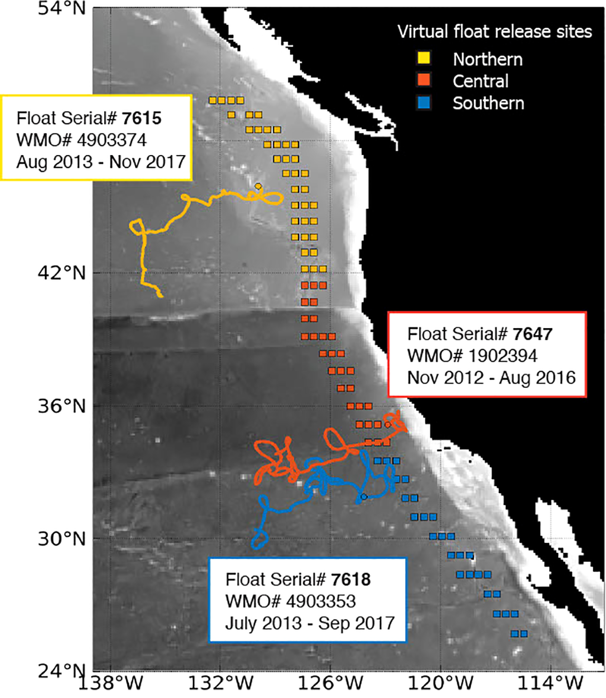
Figure 1. Map of the California Current System (CCS) showing the 92 locations where >1,600 virtual Argo floats are released, as well as the trajectories of the 3 real floats which sampled the area between 2012 and 2017. Note that, to minimize shallow (<2000 m) bottom encounters, virtual floats are released at least 60 but within 120 nautical miles from the nearest shoreline and only in waters at least 2000 m deep. Greyscale indicates ocean bottom depth, i.e., lighter color means shallower.

Sensitivity of simulated float trajectories and along-track variability to varying sampling strategies (i.e., the choice of profiling interval and parking depth) is also investigated. To do so, additional fleets of floats are deployed on July 1^st, 2012 at the same 92 locations in the CCS and simulated for 5 years in the same manner except that the parking depth is set at 200 m, 500 m, and 2000 m, respectively (n = 276), instead of the default 1000 m, and that the profiling interval is set at 1-day, 3-day, 10-day, 15-day, and 30-day, respectively (n = 460), instead of the default 5-day interval. Note that 200 m is the shallowest parking depth explored here due to the practical concern for biofouling at shallower depths. Together with the control deployments, 1,656 virtual float trajectories are analyzed in this study.

2.4 Sampled ocean physical and biogeochemical variability by real and virtual floats

We compare our model simulations against 3 real Argo floats’ physical and biogeochemical measurements along their trajectories to assess the fidelity of our model in representing real float sampling and observations. Their WMO (serial) numbers are 1902394 (7647), 4903353 (7618), and 4903374 (7615), respectively (Figure 1). These 3 floats sampled the CCS across 29-46°N and 122-136°W from 2012 to 2017 at 5-day profiling intervals, and have been previously analyzed to characterize subsurface oxygen variability in the CCS (Schultz et al., 2024). While new datasets have become available from recently deployed floats in the CCS, we focus our analysis on these 3 floats because they provide 4-5 years of physical and biogeochemical observations (i.e., temperature, chlorophyll, nitrate, and dissolved oxygen) to be compared with our long-term model simulations. Data from these floats were obtained from MBARI’s Chem Sensor Data Server (https://www.mbari.org/data/ocean-float-data/), last updated on 08/17/2023. When compared against observations, model simulated fields are first saved as daily means on pressure levels and on the model’s native grid (0.125° x 0.125°), then sampled on the day when, and at the grid point nearest to where, an observation is made along the real floats’ trajectories. This comparison is to assess the representativeness of our model in simulating the seasonal and spatial variability observed by the real floats.

Additionally, we analyze the drifts of virtual floats and the simulated physical and biogeochemical variability along the virtual floats’ trajectories. This allows us to sample model simulations in a quasi-Lagrangian sense, consistent with the model’s own flow fields. Similarly, the simulated daily means are sampled every 5 days (or at varying intervals in the sensitivity experiments) at the grid cell nearest to a virtual float’s location along its trajectory. Here, the sampling of daily mean values every 5 days, as opposed to the use of 5-day averages, is chosen to better mimic the sampling behavior of real floats.

2.5 Estimation of “eddy association” using ocean current speed anomaly

A float’s trajectory and sampled variability can be largely affected by eddy-like features that the float encounters, while the probability of a float getting entrained into an eddy and repeatedly sampling it depends on the frequency of eddy-genesis in the area, eddy translation and as well as the amount of time the float drifts at eddy-relevant depths (from surface to as deep as 1500 meters in our model; Supplementary Figure S1). Wang et al. (2020) use model simulations to find that eddies tend to accelerate floats and converge them toward regions with stronger ocean currents. Here we use the along-track ocean current speed anomaly at 500 m relative to the 9-year climatological mean to identify ocean features associated with stronger currents, such as eddies. We choose to use the 500 m velocities to identify eddies because eddy structures are more distinct at 500 m and 1000 m than at shallower and deeper depths (Supplementary Figure S1). We also note that analysis using the 500 m and 1000 m velocities show consistent results (See Section 3.3). The along-track current speed is calculated from the co-located daily velocities as the square root of (u² + v²) at 500 m and at the grid cell nearest to each location of the float, while daily climatological mean is calculated in the same manner but averaged over the 9-year period between July 2008 and June 2017. Daily standard deviation across these 9 years is calculated accordingly as well. A 3-day moving average filter is applied to the daily climatological mean and standard deviation to remove noise associated with short-term and small-scale variability. We recognize that stronger currents may be associated with not only persistent eddy-like features but also episodic features such as submesoscale fronts. We therefore consider an event having an “eddy association” only when the along-track ocean current speed anomaly is consistently greater than one standard deviation at a given location and day of the year for at least 30 days. We then estimate the total number of days for which a float is considered associated with an eddy over the 5-year period, and assess how this probability (i.e., total numbers of “eddy association” days/1826 x 100%) may be affected by the choice of float parking depth.

3 Results

3.1 Comparison of real floats’ along-track observations and model simulations

Observations from the 3 real floats are analyzed and compared with model simulations along the real floats’ trajectories, where and when measurements were made. Float #7647 was deployed in November 2012 at 35°N,123°W, approximately 70 nautical miles from the shoreline, and later ceased operations further offshore in August 2016. Float #7618 was deployed in the following summer in July 2013 at 32°N,124°W, about 180 nautical miles south of where Float #7647 was deployed. It drifted offshore to the southwest and ceased operations in September, 2017. Float #7615 was deployed a month later in August 2013 but further north in the CCS at 46°N,130°W, which also drifted to the southwest before it ceased operations in November 2017 (Figure 1). These floats were equipped with sensors for temperature, salinity, nitrate, dissolved oxygen (DO), and chlorophyll fluorescence. They profiled at 5-day intervals, providing long-term (46-51 months) datasets monitoring large-scale and seasonal variability as well as impacts of individual eddies the floats encountered as they moved from their inshore deployment locations to the southwest.

Physical and biogeochemical variability measured by these floats every 5 days along their trajectories are compared against model-simulated fields sampled at the same time and locations. Our model shows varying levels of fidelity in representing real float observations for different ocean variables and depths: While the model successfully represents float-sampled magnitude and variability of temperature at the surface for all three cases, it underrepresents the observed temperature range at the depth of 300 m by about 40% or 1°C in two of the three cases (i.e., Float #7647 and #7618, which sampled the southern and central CCS around 30-36°N; Figures 2a, b, 3a; Supplementary Figures S2a, b, S3a). Schultz et al. (2024) analyzed ocean interior temperature simulated in this model and found it less variable in the CCS when compared to two fully coupled Earth System models, both of which employed the same ocean-ice model. We thus attribute this lack of fidelity to limitations of the atmospheric reanalysis-forced, ice/ocean experimental design - while the external (e.g., wind) forcing generates circulation variability, the assumption of an infinite heat capacity atmosphere and application of salinity restoring dampens ocean internal variability through the surface (Griffies et al., 2016). The case is somewhat opposite for nitrate concentrations (Figures 2c, 3b; Supplementary Figures S2b, S3b), however, as the model retains the large-scale observed nitrate structure by capturing about 90% of the observed range in the interior but substantially underestimates both the observed range and highest values of surface nitrate concentrations by more than 50%. This discrepancy is largely due to weaker coastal upwelling and consequently a deeper nutricline in the model when compared to observations. For example, several strong coastal upwelling events occurred in the central CCS in the early seasons of 2013, which acted to bring high concentrations of nitrate up to the surface. This upwelling was successfully captured by Float #7647 sampling in the area but is not seen in the model (Figure 3b). Nonetheless, the model successfully represents the CCS nutricline depth and its variability over most parts of the float trajectories (Figure 3b). For chlorophyll, in addition to underrepresenting the dynamic range and highest surface values (Figure 2d), the model also underestimates the depth extent of chlorophyll and the potential for significant measurable chlorophyll far below the euphotic zone. The former we interpret as a model deficiency in representing high chlorophyll content in living phytoplankton cells under low light conditions, while the latter suggests the presence of fluorescence in slowly sinking particles, which is not represented in the model. Additionally, van Oostende et al. (2018) suggests that implementing a fast growing (e.g., coastal diatom) phytoplankton type in COBALT allows the model to better capture the productive endpoints of chlorophyll observed in the CCS, which is lacking in the version of COBALT used in this study. Modeled DO variability is driven by a combination of its temperature and nutrient controls with good correspondence in the surface as a function of temperature, but damped variability at depth likely due to underrepresentation of temperature variability (Figures 2b, e, 3a, d; Supplementary Figures 2b, c, 3, 4b, d, 5a, c). Overall, the model captures only about 60% of the observed temperature variability but >85% of DO variability in the ocean interior.

Figure 2

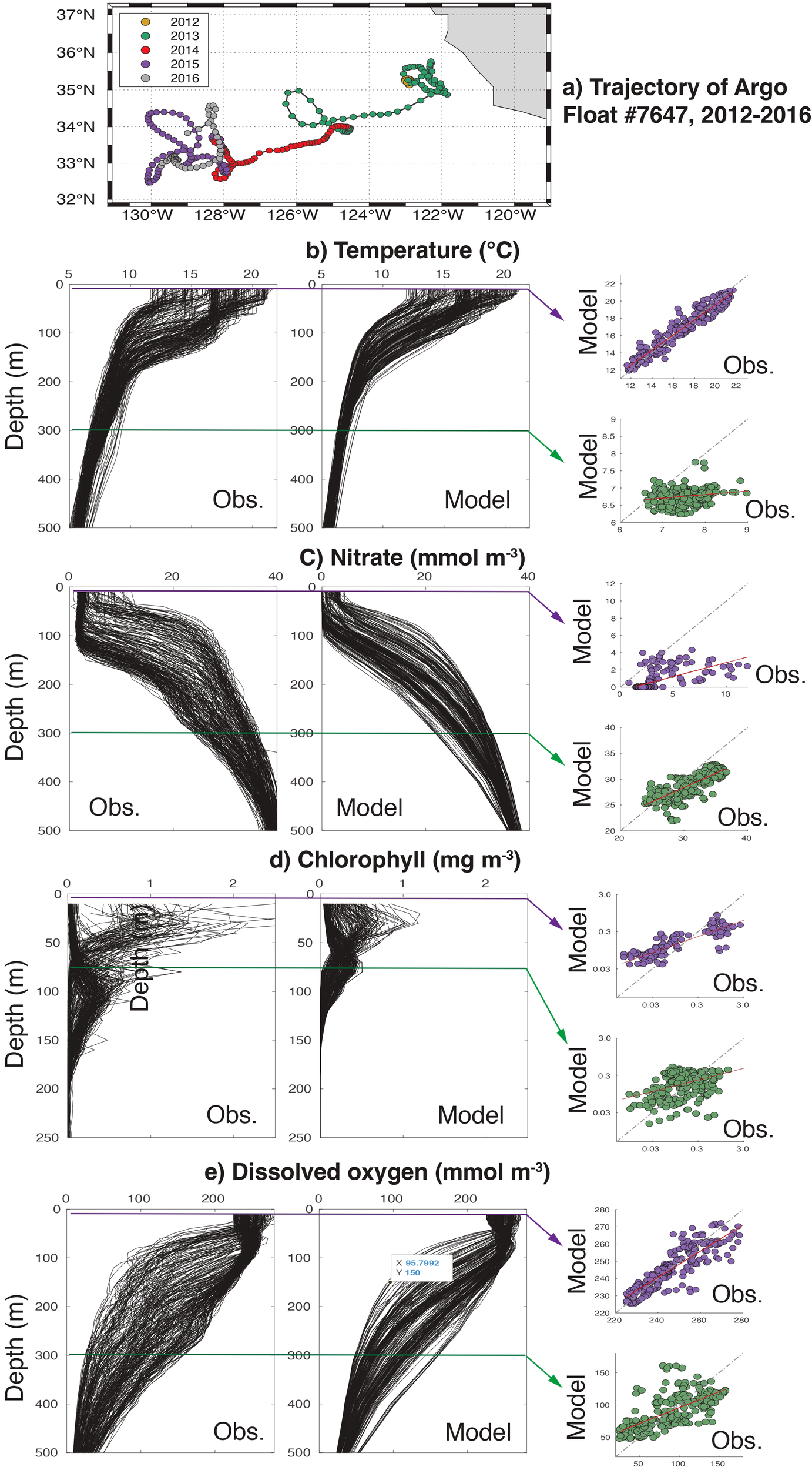
Figure 2. (a) Trajectory of a real float (Series# 7647, WMO# 1902394) deployed in the CCS, which provided a 46-month dataset of sampled ocean physical and biogeochemical variability along its trajectory, and comparisons of Float #7647 measured profiles and model-simulated profiles of (b) temperature, (c) nitrate concentration, (d) chlorophyll concentration, and (e) dissolved oxygen concentration in the upper 500 m sampled at the same time and locations of the real float’s observations.

Figure 3

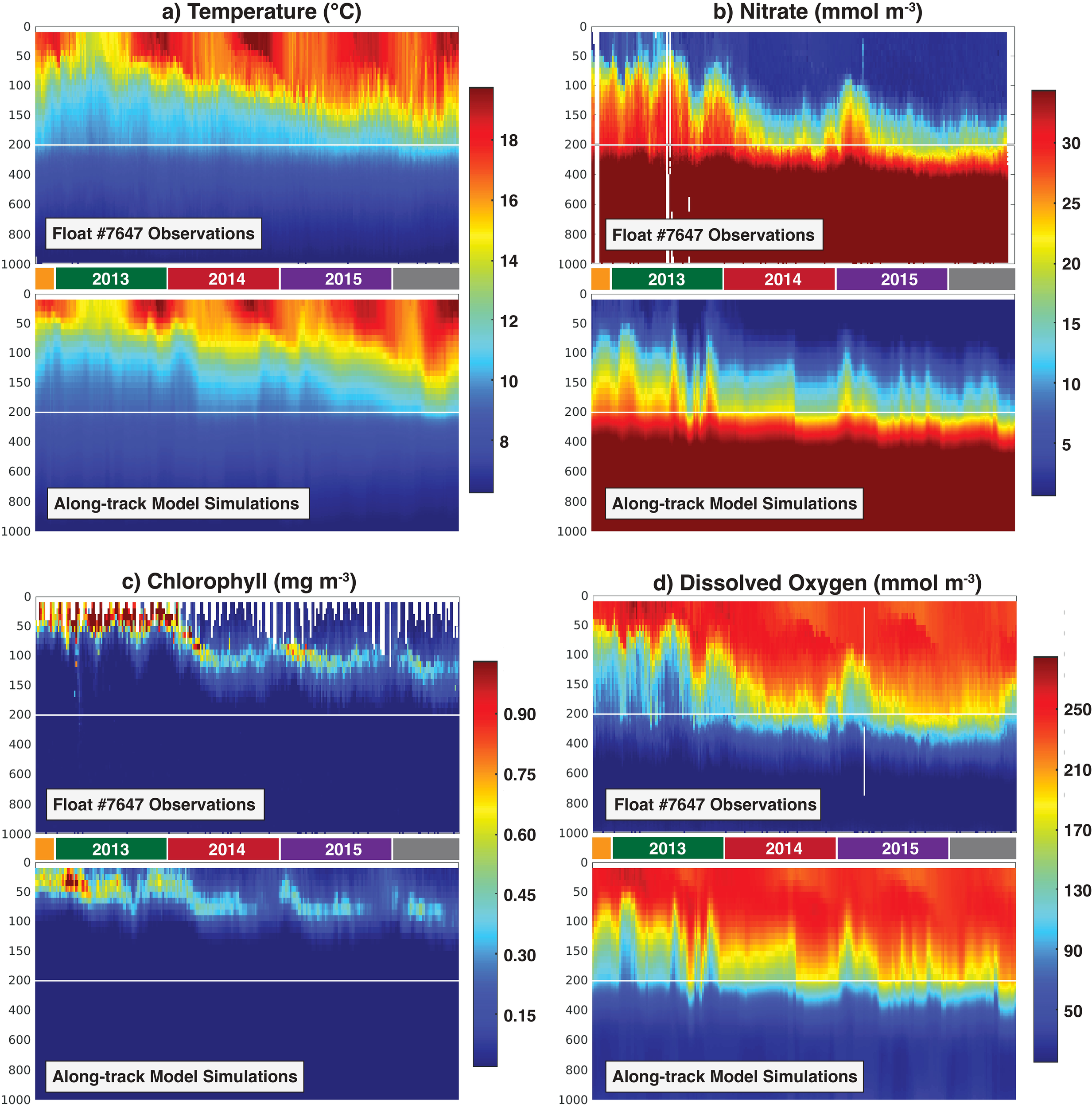
Figure 3. Comparison of Float #7647 measured and model simulated (a) temperature, (b) nitrate, (c) chlorophyll concentration, and (d) dissolved oxygen concentration at the same time and locations along the real float’s trajectory over the 46-month period between 2012 and 2016.

3.2 Sensitivity of simulated float trajectories and sampled variability to deployment location

Beyond the chaotic influence of eddies and fronts, the overall direction and offshore extent of simulated float trajectories show a noticeable dependency on the latitude of the deployment sites (Figures 4a–c). To quantify and visualize the spatial spans and the likelihood of an average float drifting to, and sampling a given location, we use density plots (Figures 4d–f) to show the total number of profiles collected by the float ensemble in a given gridded location during the entire period scaled by the size of the float ensemble (n = 920). A denser distribution thus indicates a higher probability for this location to be sampled by the floats. For example, a high density of 7 on the map means that an average float deployed nearshore within this domain is expected to drift to, and stay at that location for about 35 days, and collect 7 profiles there across its 5-year lifespan. Floats deployed in the northern domain (i.e., north of 42°N) tend to drift to the northwest and stay relatively inshore (Figures 4c, f). This pattern is likely driven by seasonally consistent northwestward coastal currents at the floats’ drifting depth of 1000 m, and strong summertime surface currents of the same direction (Supplementary Figure S6). Floats deployed in the central areas (34-42°N) tend to drift offshore overall but may spread extensively to the north and southwest as well, covering an approximately 40% larger area than those from the more northerly deployments (Figures 4b, e, h). These offshore drifts and areal coverage patterns are consistent between summertime and wintertime deployments even though the ocean current system undergoes a seasonal reversal in the central CCS (Supplementary Figures S7, S8). While it is unclear whether the 1000-m current fields dominate the drift, the strong wintertime southwestward surface currents may also play an important role (Supplementary Figure S6). Floats deployed further south (south of 34°N) tend to drift offshore to the southwest though to a lesser extent compared to the central CCS deployments (Figure 4a). This finding is consistent with the direction of wintertime surface currents and, further in the south, summertime surface currents as well (Supplementary Figure S6). The areal coverage of these floats is similar to those from the northerly deployments (Figures 4g, h).

Figure 4

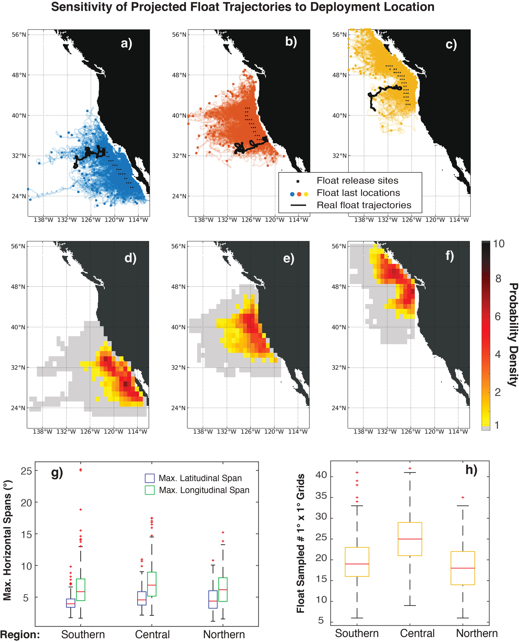
Figure 4. (a-c) Overall drift direction and extent and (d-f) spatial probability density distribution of simulated float trajectories, (g) maximum latitudinal and longitudinal spans of float drift, and (h) areal coverage by the floats over the 5-year period, showing the sensitivity to the latitude of deployment locations in the CCS. Floats are grouped into the southern (floats deployed between 25.9-34°N), central (34-42°N), and northern (42-50°N) deployment domains (control deployments, n = 920).

Controls of float sampled variability of temperature, nitrate, chlorophyll, and DO at the ocean surface and interior include local spatiotemporal gradients in model simulated fields and float sampled area associated with the direction and offshore extent of the drift. Overall, floats from more northerly deployments sampled a larger surface range in temperature (~6°C) and chlorophyll (~0.7 mg m^-3) compared to those from more southerly deployments (Figures 5a, c). In the ocean interior, float sampled variability appears less sensitive to the latitudes of the deployment sites. However, larger ranges of nitrate and DO at depths of 200-300 m are captured by floats deployed in the central and southern regions, consistent with the overall larger area sampled by these floats (Figures 4h, 5b, d).

Figure 5

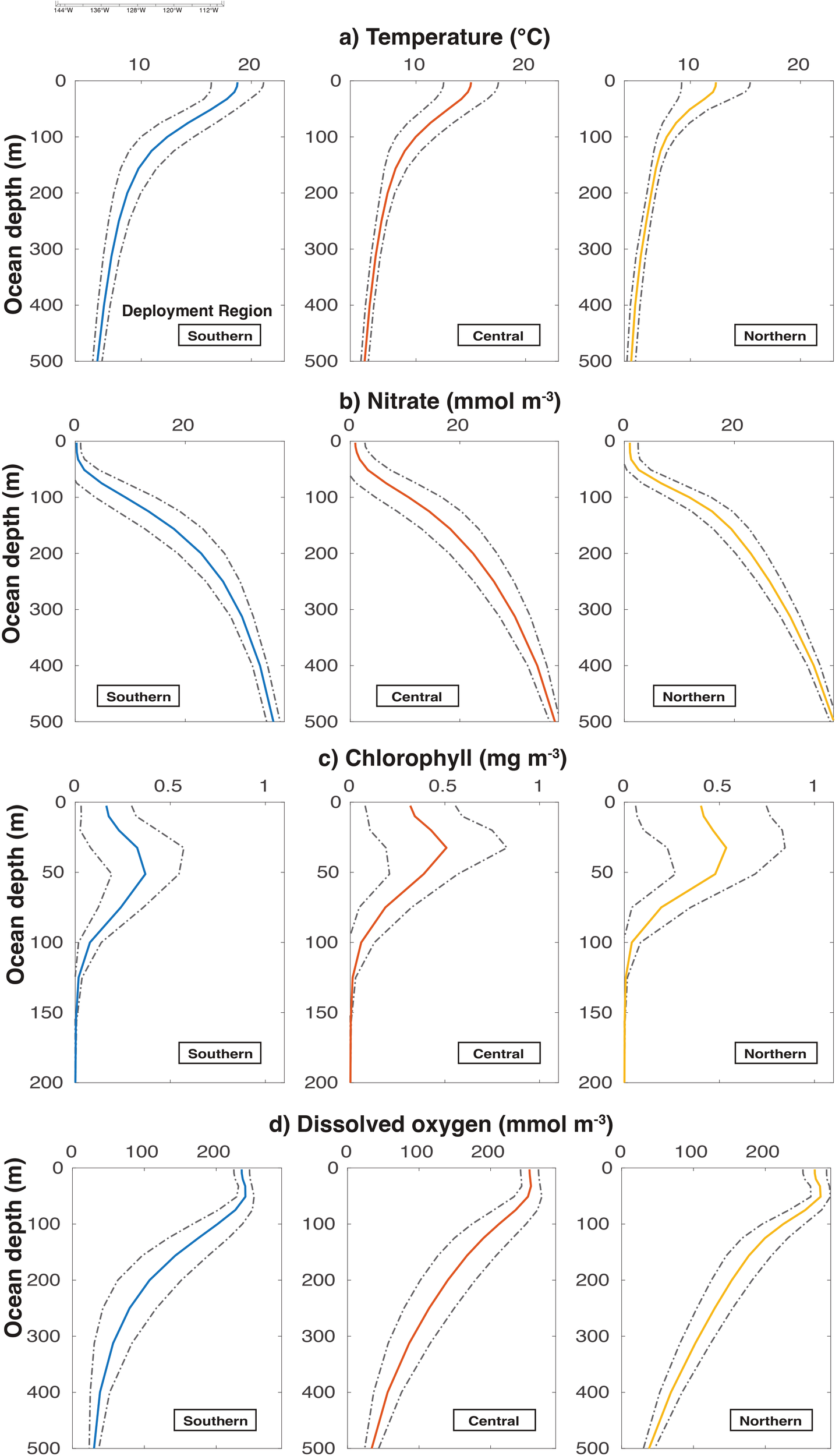
Figure 5. Virtual float sampled profiles of (a) temperature, (b) nitrate concentration, (c) chlorophyll concentration, and (d) dissolved oxygen concentration in the upper 500 m and their sensitivity to the latitude of deployment locations. Each solid line represents the mean values averaged over about 109,500 profiles (i.e., for the control deployments, there are a total of about 300 floats deployed in each domain and each float sampled about 365 profiles), and the dashed lines represent one standard deviation from the mean values.

3.3 Sensitivity of simulated float trajectories and sampled variability to parking depth

Simulated float trajectories and sampled variability in temperature, nitrate, chlorophyll, and DO depend largely on the depth at which floats spend a majority of their lifetime drifting. When operating on a 5-day profiling cycle, for example, a float spends 4.5 days or 90% time drifting at its parked depth. Three additional float fleets are deployed at the same 92 locations (n = 276) as a sensitivity experiment in which these floats’ parking depth is altered from the default 1000 m to 200 m, 500 m, and 2000 m, respectively, to assess the sensitivity of simulated trajectories and sampled variability to this change (Figures 6–8). Simulated trajectories show that floats drifting at 2000 m move a much shorter distance on average over the 5-year period, essentially providing a nearly Eulerian dataset (Figure 6d), while floats drifting at 200 m, 500 m and 1000 m provide datasets associated with stronger mean currents and more eddy-like features which they encounter at shallower depths (Figures 6a–c, 7c). Maximum latitudinal and longitudinal drift spans and areal coverage over the 5-year period all decrease as the parking depth increases (Figures 6e, f), largely due to stronger mean currents at shallower depths (Supplementary Figure S1). However, analyzing the along-track ocean current speed anomaly at a given location and day of the year (see Section 2.5) suggests that floats drifting at shallower depths do not necessarily experience stronger-than-usual currents (Figure 7c). The probability of a float getting entrained into and repeatedly sampling an eddy-like feature is 50% higher for the 1000-m drifting case when compared to the 200-m drifting case despite a larger sampled area and a stronger mean flow experienced by the latter, followed by the 500-m and 2000-m drifting cases (Figure 7c). An analysis using the 1000 m velocities to identify eddy-like structures, as opposed to the 500 m velocities, are provided in Supplementary Figure S9 and shows consistent results.

Figure 6

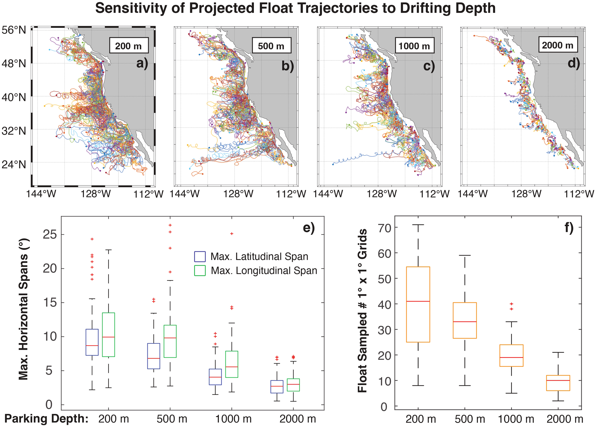
Figure 6. (a-d) Overall drift direction and extent of simulated float trajectories, (e) maximum latitudinal and longitudinal spans of float drift, and (f) areal coverage by the floats over the 5-year period, showing the sensitivity to different parking depths (200 m, 500 m, 1000 m, and 2000 m; n = 368). In a-d, colored lines are used to simply differentiate the numerous floats.

Figure 7

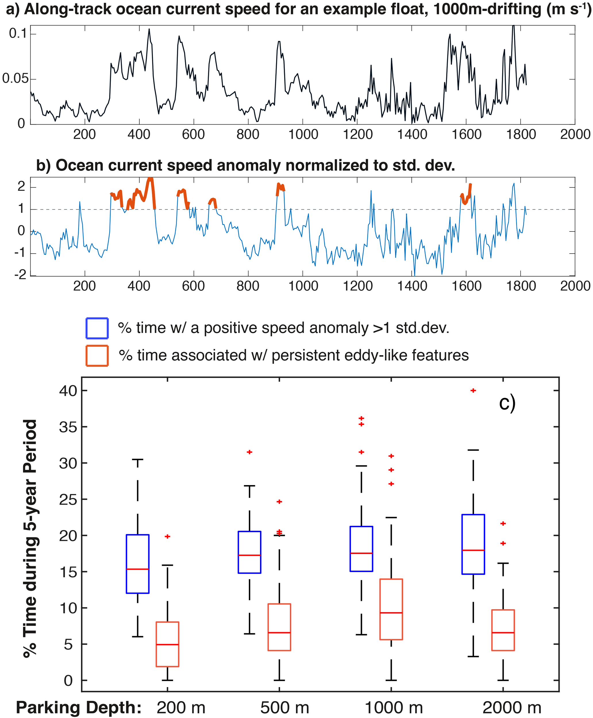
Figure 7. (a) An example showing daily ocean current speed along the trajectory of a 1000-m drifting float over the 5-year period. (b) Identification of the total number of days, shown in thickened red segments, when the float is considered associated with and repeatedly sampling the same eddy-like features using the ocean current speed anomaly criteria (see Section 2.5). (c) % time an average float experiences stronger-than-usual ocean currents, shown in blue boxes, and % time an average float is considered associated with and repeatedly sampling the same eddy-like features, shown in orange boxes, over the 5-year period, as well as their sensitivity to different parking depths (200 m, 500 m, 1000 m, and 2000 m; n = 368).

Figure 8

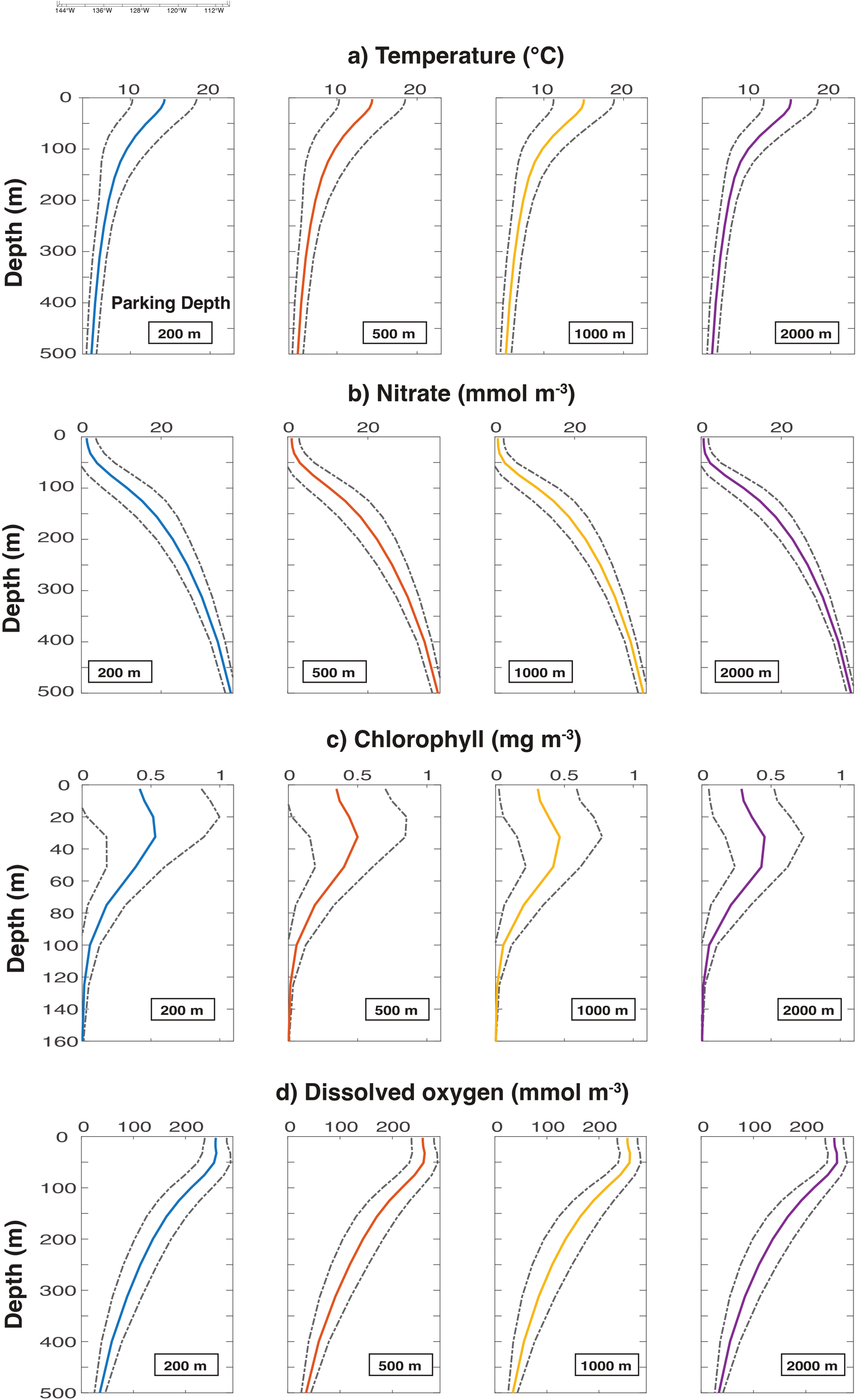
Figure 8. Virtual float sampled profiles of (a) temperature, (b) nitrate concentration, (c) chlorophyll concentration, and (d) dissolved oxygen concentration in the upper 500 m and their sensitivity to parking depth. Each solid line represents the mean value averaged over 33,580 profiles, i.e., there are 92 floats deployed in all three (northern, central, southern) regions in each experiment, and each float collected about 365 profiles, and dashed lines represent one standard deviation from the mean values.

Due to the aforementioned, these datasets sample the area and its variability quite differently as they not only sample the Eulerian and Lagrangian variability at different depths but also have an up to 10% probability of continuously quasi-Lagrangian sampling the same eddy-like features for prolonged periods. Overall, sampled dynamic ranges in surface ocean temperature, nitrate, chlorophyll, and DO all increase in the 200 m-drifting dataset as the floats move further to the southwest and sample a broader area along their trajectories, in particular for chlorophyll ranges. Higher chlorophyll mean values (>0.5 mg m^-3) are also sampled in the upper 50 m with 200-m drifting but not in the deeper-drifting cases (Figure 8c). Temperature, nitrate, and DO, in contrast, do not exhibit a difference in mean sampled values across all cases either at the surface or in the interior (Figures 8a, b, d).

3.4 Sensitivity of simulated float trajectories and sampled variability to profiling and sampling intervals

In contrast to the high sensitivity to parking depth, sensitivity to profiling intervals across 1 to 30 days appears low with regard to both simulated float drift spans and coverage area (Supplementary Figures S10-S12). We also assess the degree to which more frequent sampling (i.e., how often the sensors are turned on) can better capture the full range of variability in float observables. To test this sensitivity of sampled variability to sampling intervals, we analyze the fleet of floats set to a daily profiling interval and compute the sampled ranges of daily temperature, nitrate, chlorophyll, and DO for the 5-year period (n = 92). This dataset is considered to contain the full range of observed variability. We then reduce the sampling interval from daily to the typical float sampling intervals (every 5-10 days), sub-seasonal (every 30 days), seasonal (every 90 days), and interannual (every 365 days), and compute the percentage of retained sampled range compared to the full range dataset. Sampling at typical intervals (every 5-10 days) still captures over 75% of the daily surface variability in all ocean variables, while interannual variability from sampling every 365 days accounts for about 20% of daily surface variability (Figure 9). For the ocean interior, the typical 5-10 days sampling design captures over 80% of daily variability for temperature, 87% for chlorophyll, and over 95% for nitrate and DO in good correspondence to their solubility and biogeochemical controls.

Figure 9

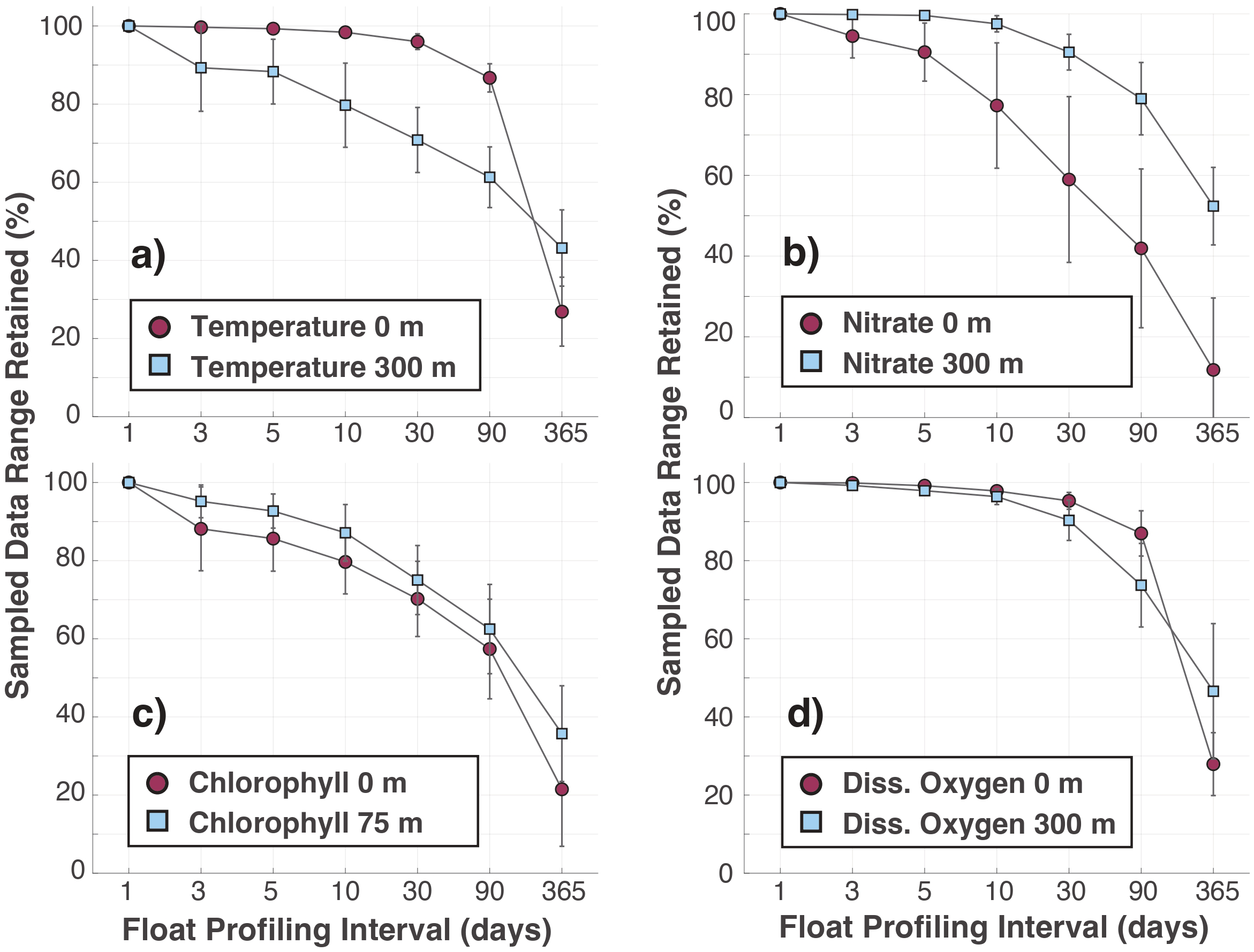
Figure 9. Sensitivity of float sampled range of (a) temperature, (b) nitrate concentration, (c) chlorophyll concentration, and (d) dissolved oxygen concentration at the ocean surface and interior to float sampling intervals, shown as the percentage of sampled range retained compared to the daily sampling dataset. For each float, a sampled dataset comprises {VAR_sday, VAR_sday+n, VAR_sday+2n, …}, where VAR is the sampled ocean variable, sday is the first day of sampling which can be {1, 2, …, n-1}, and n is the sampling interval in days. The range (i.e., maximum value - minimum value) of the sampled dataset is computed for each sday and then the mean and standard deviation of all the sampled ranges are computed. The mean sampled range for each VAR and each sampling interval, shown as a filled circle for the surface and a filled square for the ocean interior, and the mean standard deviation, shown as the length of an error bar, are averaged values across all floats (n = 92).

4 Discussion and conclusions

Our initial finding is that most virtual floats deployed in the CCS tend to drift offshore to the southwest even though the current system undergoes a seasonal reversal, which is consistent with the trajectories of all 3 real floats analyzed. Taking a closer look, however, we find a strong latitudinal dependency of the overall directions and offshore extent of the float trajectories. Floats deployed in the north tend to drift to the northwest and stay relatively inshore; floats deployed in the central domain drift offshore overall but spread extensively to the north and the southwest while sampling the largest area and variability; floats deployed further south tend to drift offshore to the southwest. Another key finding of our analysis is that float sampled area and ocean variability are tightly linked to the parking depth and the possibility of eddy association. Because of the use of the 1000-m parking depth, floats tend to spend considerable time sampling the same eddy-like features up to a few months at a time (Figures 7b, c), making the data from these profiles highly correlated during these times and potentially limiting the total amount of variability that the floats experience over their lifetime. We recommend that this “non-random” repeated sampling of the same eddies be quantified with a spectral analysis to separate the seasonal/spatial and eddy components. While this potential for eddy-association may diminish the float’s capability of sampling the full range of variability in the local region, it also provides a quasi-Lagrangian opportunity for mechanistic analysis of biogeochemical processes within these environments over time with increased ability to interpret time-evolving concentrations into fluxes (Bushinsky et al., 2019; Gray, 2023). Encouragingly, we find little sensitivity of the floats’ trajectories and areal coverage to the frequency of profiling which supports the Argo float’s 5-day or 10-day cycle design. While we find 10-day sampling to only capture about 80% of daily variability in modeled temperature in the interior ocean at 300 m, we find higher percentages of daily variability captured for the biogeochemical variables (chlorophyll, nitrate, DO), providing support that Argo float’s standard of 5-day or 10-day sampling is also sufficient to characterize biogeochemical variability as well as physical variability. Finally, we recognize that the evaluation and analysis of these float simulations apply only to the CCS; however, our methods and recommendations may be considered more widely in similar eastern boundary current regions, in particular when considering the likelihood of float-eddy association and role of parking depth.

Data availability statement

The raw data supporting the conclusions of this article will be made available by the authors, without undue reservation.

Author contributions

XL: Data curation, Formal analysis, Methodology, Visualization, Writing – original draft. JD: Conceptualization, Funding acquisition, Methodology, Project administration, Resources, Supervision, Writing – review & editing. ED: Methodology, Writing – review & editing. GJ: Funding acquisition, Methodology, Project administration, Writing – review & editing.

Funding

The author(s) declare that financial support was received for the research and/or publication of this article. This report was prepared by Xiao Liu under award NA21OAR4310251 from the National Oceanic and Atmospheric Administration, U.S. Department of Commerce. The statements, findings, conclusions, and recommendations are those of the authors and do not necessarily reflect the views of the National Oceanic and Atmospheric Administration, or the U.S. Department of Commerce. PMEL contribution number 6454.

Acknowledgments

We thank NOAA GFDL’s M. Harrison and K. Noh who performed an internal review for an earlier draft of this manuscript, and the two journal reviewers who provided constructive insights and suggestions.

Conflict of interest

The authors declare that the research was conducted in the absence of any commercial or financial relationships that could be construed as a potential conflict of interest.

Publisher’s note

All claims expressed in this article are solely those of the authors and do not necessarily represent those of their affiliated organizations, or those of the publisher, the editors and the reviewers. Any product that may be evaluated in this article, or claim that may be made by its manufacturer, is not guaranteed or endorsed by the publisher.

Supplementary material

The Supplementary Material for this article can be found online at: https://www.frontiersin.org/articles/10.3389/fmars.2025.1481761/full#supplementary-material

References

Adcroft A., Anderson W., Balaji V., Blanton C., Bushuk M., Dufour C. O., et al. (2019). The GFDL global ocean and sea ice model OM4.0: Model description and simulation features. J. Adv. Modeling Earth Syst. 11, 3167–3211. doi: 10.1029/2019MS001726

Crossref Full Text | Google Scholar

Addey C. I. (2022). Using Biogeochemical Argo floats to understand ocean carbon and oxygen dynamics. Nat. Rev. Earth Environ. 3, 739. doi: 10.1038/s43017-022-00341-5

Crossref Full Text | Google Scholar

Bograd S. J., Castro C. G., Di Lorenzo E., Palacios D. M., Bailey H., Gilly W., et al. (2008). Oxygen declines and the shoaling of the hypoxic boundary in the California Current, Geophys. Res. Lett. 35, L12607. doi: 10.1029/2008GL034185

Crossref Full Text | Google Scholar

Brady R. X., Lovenduski N. S., Yeager S. G., Long M. C., Lindsay K. (2020). Skillful multiyear predictions of ocean acidification in the California Current System. Nat. Commun. 11, 2166. doi: 10.1038/s41467-020-15722-x

Crossref Full Text | Google Scholar

Bushinsky S. M., Landschützer P., Rödenbeck C., Gray A. R., Baker D., Mazloff M. R., et al. (2019). Reassessing Southern Ocean air-sea CO2 flux estimates with the addition of biogeochemical float observations. Global Biogeochemical Cycles 33.11, 1370–1388. doi: 10.1029/2019GB006176

Crossref Full Text | Google Scholar

Chan F., Barth J. A., Lubchenco J., Kirincich A., Weeks H., Peterson W. T., et al. (2008). Emergence of anoxia in the California Current large marine ecosystem. Science 319, 920. doi: 10.1126/science.1149016

Crossref Full Text | Google Scholar

Chavez F., Messie M. (2009). A comparison of eastern boundary upwelling ecosystems. Prog. Oceanogr 83, 80–96. doi: 10.1016/j.pocean.2009.07.032

Crossref Full Text | Google Scholar

Checkley D., Barth J. A. (2009). Patterns and processes in the california current system. Prog. Oceanogr. 83, 49–64. doi: 10.1016/j.pocean.2009.07.028

Crossref Full Text | Google Scholar

Dussin R., Curchitser E. N., Stock C. A., Van Oostende N. (2019). Biogeochemical drivers of changing hypoxia in the California Current Ecosystem. Deep-Sea Res. II 169–170, 104590. doi: 10.1016/j.dsr2.2019.05.013

Crossref Full Text | Google Scholar

Feely R. A., Okazaki R. R., Cai W.-J., Bednaršek N., Alin S. R., Byrne R. H., et al. (2018). The combined effects of acidification and hypoxia on pH and aragonite saturation in the coastal waters of the California current ecosystem and the northern Gulf of Mexico, Cont. Shelf Res. 152, 50–60. doi: 10.1016/j.csr.2017.11.002

Crossref Full Text | Google Scholar

Galán A., Saldías G. S., Corredor-Acosta A., Muñoz R., Lara C and Iriarte J. L. (2021). Argo float reveals biogeochemical characteristics along the freshwater gradient off western patagonia. Front. Mar. Sci. 8. doi: 10.3389/fmars.2021.613265

Crossref Full Text | Google Scholar

Garcia H. E., Locarnini R. A., Boyer T. P., Antonov J. I., Baranova O. K., Zweng M. M., et al. (2014a). World Ocean Atlas 2013, Volume 3: Dissolved Oxygen, Apparent Oxygen Utilization, and Oxygen Saturation. In Levitus S., Mishonov A. Ed. NOAA Atlas NESDIS 75, 27 pp. National Oceanic and Atmospheric Administration, Silver Spring, MD, USA.

Google Scholar

Garcia H. E., Locarnini R. A., Boyer T. P., Antonov J. I., Baranova O. K., Zweng M. M., et al. (2014b). “World ocean atlas 2013, Volume 4: Dissolved inorganic nutrients (phosphate, nitrate, silicate),” in NOAA atlas NESDIS, vol. 76 . Eds. Levitus S., Mishonov &A., 25). National Oceanic and Atmospheric Administration, in Silver Spring, MD, USA.

Google Scholar

Gray A. R. (2024). The four-dimensional carbon cycle of the southern ocean. Ann Rev Mar Sci. 16:163–190. doi: 10.1146/annurev-marine-041923-104057

PubMed Abstract | Crossref Full Text | Google Scholar

Griffies S. M., Danabasoglu G., Durack P. J., Adcroft A. J., Balaji V., Böning C. W., et al. (2016). OMIP contribution to CMIP6: Experimental and diagnostic protocol for the physical component of the Ocean Model Intercomparison Project. Geoscientific Model. Dev. 3231–3296. doi: 10.5194/gmd-9-3231-2016

Crossref Full Text | Google Scholar

Gruber N., Hauri C., Lachkar Z., Loher D., Frölicher T. L., Plattner G. K. (2012). Rapid progression of ocean acidification in the California Current System. Science. 337, 220–223. doi: 10.1126/science.1216773

PubMed Abstract | Crossref Full Text | Google Scholar

Hickey B., MacFadyen A., Cochlan W., Kudela R., Bruland K., Trick C. (2006). Evolution of chemical, biological and physical water properties in the northern California current in 2005: Remote or local wind forcing? Geophysical Res. Lett. 33. doi: 10.1029/2006GL026782

Crossref Full Text | Google Scholar

Huyer A. (1983). Coastal upwelling in the California Current system. Prog. Oceanography 12, 259–284. doi: 10.1016/0079-6611(83)90010-1

Crossref Full Text | Google Scholar

Johnson K. S., Bif M. B. (2021). Constraint on net primary productivity of the global ocean by Argo oxygen measurements. Nat. Geosci. 14, 769–774. doi: 10.1038/s41561-021-00807-z

Crossref Full Text | Google Scholar

Johnson G. C., Hosoda S., Jayne S. R., Oke P. R., Riser S. C., Roemmich D., et al. (2022). Argo–two decades: Global oceanography, revolutionized. Annu. Rev. Mar. Sci. 14, 379–403. doi: 10.1002/2016GL070413

Crossref Full Text | Google Scholar

Kudela R. M., Banas N. S., Barth J. A., Frame E. R., Jay D. A., Largier J. L., et al. (2008). New insights into the controls and mechanisms of plankton productivity in coastal upwelling waters of the Northern California Current System. Oceanography 21, 46–59. doi: 10.5670/oceanog.2008.04

Crossref Full Text | Google Scholar

Liu X., Stock C. A., Dunne J. P., Lee M., Shevliakova E., Malyshev S., et al. (2021). Simulated global coastal ecosystem responses to a half-century increase in river nitrogen loads. Geophys. Res. Lett. 48, e2021GL094367. doi: 10.1029/2021GL094367

Crossref Full Text | Google Scholar

Locarnini R. A., Mishonov A. V., Antonov J. I., Boyer T. P., Garcia H. E., Baranova O. K., et al. (2013). “World ocean atlas 2013, Volume 1: Temperature,” in NOAA atlas NESDIS, vol. 73 . Eds. Levitus S., Mishonov &A., 40. National Oceanic and Atmospheric Administration, in Silver Spring, MD, USA.

Google Scholar

Mazloff M. R., Verdy A., Gille S. T., Johnson K. S., Cornuelle B., Sarmiento J. (2023). Southern Ocean acidification revealed by biogeochemical-Argo floats. J. Geophysical Research: Oceans 128, e2022JC019530. doi: 10.1029/2022JC019530

Crossref Full Text | Google Scholar

McClatchie S., Goericke R., Cosgrove R., Auad G., Vetter R. (2010). Oxygen in the Southern California Bight: Multidecadal trends and implications for demersal fisheries, Geophys. Res. Lett. 37, L19602. doi: 10.1029/2010GL044497

Crossref Full Text | Google Scholar

Olsen A., Key R. M., van Heuven S., Lauvset S. K., Velo A., Lin X., et al. (2016). The Global Ocean Data Analysis Project version 2 (GLODAPv2) – An internally consistent data product for the world ocean. Earth System Sci. Data 8, 297–323. doi: 10.5194/essd-8-297-2016

Crossref Full Text | Google Scholar

Roemmich D., Alford Matthew H., Hervé C., Kenneth J., King B., Moum J., et al. (2019). On the future of argo: A global, full-depth, multi-disciplinary array. Front. In Mar. Sci. 6, 28. doi: 10.3389/fmars.2019.00439

Crossref Full Text | Google Scholar

Santora J. A., Mantua N. J., Schroeder I. D., Field J. C., Hazen E. L., et al. (2020). Habitat compression and ecosystem shifts as potential links between marine heatwave and record whale entanglements. Nat. Commun. 11, 536. doi: 10.1038/s41467-019-14215-w

PubMed Abstract | Crossref Full Text | Google Scholar

Schultz C., Dunne J. P., Liu X., Drenkard E., Carter B. (2024). Characterizing subsurface oxygen variability in the California Current System (CCS) and its links to water mass distribution. J. Geophysical Research: Oceans 129, e2023JC020000. doi: 10.1029/2023JC020000

Crossref Full Text | Google Scholar

Smith J. A., Buil M. P., Muhling B., Tommasi D., Brodie S., Frawley T. H., et al. (2023). Projecting climate change impacts from physics to fisheries: A view from three California current fisheries. Prog. Oceanography 211, 102973. doi: 10.1016/j.pocean.2023.102973

Crossref Full Text | Google Scholar

Stock C. A., Dunne J. P., Fan S., Ginoux P., John J., Krasting J., et al. (2020). Ocean biogeochemistry in GFDL’s Earth System Model 4.1 and its response to increasing atmospheric CO2. J. Adv. Modeling Earth Syst. 12, e2019MS002043. doi: 10.1029/2019MS002043

Crossref Full Text | Google Scholar

Tsujino H., Urakawa S., Nakano H., Small R. J., Kim W. M., Yeager S. G., et al. (2018). JRA-55 based surface dataset for driving ocean–sea-ice models (JRA55-do). Ocean Modell 130, 79–139. doi: 10.1016/j.ocemod.2018.07.002

Crossref Full Text | Google Scholar

van Oostende N., Dussin R., Stock C., Barton A., Curchitser E., Dunne J., et al. (2018). Simulating the ocean’s chlorophyll dynamic range from coastal upwelling to oligotrophy. Prog. Oceanography 168, 232–247. doi: 10.1016/j.pocean.2018.10.009

Crossref Full Text | Google Scholar

Wang T. Y., Gille S. T., Mazloff M. R., Zilberman N., Du Y. (2018). Numerical simulations to project Argo float positions in the mid-depth and deep southwest Pacific. J. Atmospheric Oceanic Technol. 35, 1425–1440. doi: 10.1175/JTECH-D-17-0214.1

Crossref Full Text | Google Scholar

Wang T., Gille S. T., Mazloff M. R., Zilberman N. V., Du Y. (2020). Eddy-induced acceleration of Argo floats. J. Geophysical Research: Oceans 125, e2019JC016042. doi: 10.1029/2019JC016042

Crossref Full Text | Google Scholar

Weber E. D., Auth T. D., Baumann-Pickering S., Baumgartner T. R., Bjorkstedt E. P., Bograd S. J., et al. (2021). State of the California current 2019–2020: Back to the future with marine heatwaves? Front. Mar. Sci. 8. doi: 10.3389/fmars.2021.709454

Crossref Full Text | Google Scholar

Xing X., Wells M. L., Chen S., Lin S., Chai F. (2020). Enhanced winter carbon export observed by BGC-Argo in the Northwest Pacific Ocean. Geophysical Res. Lett. 47, e2020GL089847. doi: 10.1029/2020GL089847

Crossref Full Text | Google Scholar

Zhang Y., Bai Y., He X., Li T., Jiang Z., Gong F. (2023). Three stages in the variation of the depth of hypoxia in the California Current System 2003-2020 by satellite estimation. Sci. Total Environ. 874, 162398. doi: 10.1016/j.scitotenv.2023.162398

PubMed Abstract | Crossref Full Text | Google Scholar

Zweng M. M., Reagan J. R., Antonov J. I., Locarnini R. A., Mishonov A. V., Boyer T. P., et al. (2013). “World ocean atlas 2013, Volume 2: Salinity,” in NOAA atlas NESDIS, vol. 74 . Eds. Levitus S., Mishonov &A., 39. National Oceanic and Atmospheric Administration, in Silver Spring, MD, USA.

Google Scholar