Abstract
Ocean moored buoys are essential ocean monitoring devices that are permanently moored in the sea to collect real-time hydrological and meteorological data. In response to the anomalies and missing data in datasets collected from ocean moored buoys, this paper innovatively established an intelligent quality control Transformer-Encoder-BiLSTM model. This model can impute missing data and identify anomalies in buoy datasets. The model first uses the multi-head attention mechanism of the Transformer Encoder to extract global features from time-series data of buoy observations. Subsequently, it utilizes the BiLSTM network for temporal reasoning training to capture dynamic changes within the time series, predicted data. Finally, using the predicted data as a benchmark, the model conducts anomaly detection, fills in missing values, and rectifies stuck values. We conducted a series of comprehensive experiments, with the data from Buoy No. 0199 in Qingdao, China as an illustrative example. The experimental results indicate that the performance indicator R² of the model is above 0.9, the accuracy of quality control is above 97%, while both precision and recall are above 84%. The F1 scores range between 81.61% and 90.09%. These experiments demonstrate that this method exhibits high accuracy and efficiency in filling in missing data, rectifying stuck values and identifying anomalous data, showing broad application potential.
1 Introduction
Ocean moored buoys are crucial monitoring devices for collecting ocean observation data, which are equipped with various marine sensors to meet monitoring needs such as marine meteorological observations, ecological environmental protection, and disaster prevention and reduction. Anchored buoys provide a reliable platform for collecting and transmitting real-time hydrological and meteorological data from the ocean, characterized by their long-term, continuous, and stable nature (Liu et al., 2023). Meanwhile, anchored buoys provide robust empirical data for complex oceanographic processes, thereby advancing the development of marine science (Rapizo et al., 2015; Wang et al., 2016). In the context of developing cutting-edge marine science, the quality of firsthand ocean observation data directly determines the feasibility of constructing an accurate and reliable marine database, which is crucial for conducting marine scientific research (Wong et al., 2020; Wen et al., 2021). However, the data collected by ocean moored buoys often suffer from various issues in practical applications, such as sensor equipment failures, electromagnetic environmental interference, and component aging. These issues lead to decreased data quality, resulting in data drift, fixed values, missing values, and spike anomalies, severely affecting the accuracy and credibility of marine scientific research (Vieira et al., 2020; Martínez-Osuna et al., 2021). Therefore, there is an urgent need for standardized data processing procedures and quality control (QC) methods to fully utilize the data collected by the buoys and ensure its high quality (Zhou et al., 2018; Tan et al., 2021). The QC for the monitoring data of ocean moored buoys is a crucial issue that not only attracts the attention of data users but also becomes the focus of buoy equipment developers. After all, the quality of the data directly reflects the effectiveness of the observations made by the buoy equipment, determining whether it can accurately capture the dynamics of the ocean and provide reliable evidence for various marine research and practical applications.
Manual, semi-automatic, and visual QC are classic data QC techniques that have been successfully implemented in major international and EU marine data infrastructures, such as the World Ocean Database (WOD) (Palmer et al., 2018), the Copernicus Marine Environment Monitoring Service (CMEMS) (von Schuckmann et al., 2017), the International Quality Controlled Ocean Database (IQuOD) (Cowley et al., 2021), and the SeaDataNet (SDN) (Schaap and Lowry, 2010), etc. Although these techniques can eliminate gross errors, the data products generated still contain data anomalies, with bad data being mislabeled as good data. Traditional methods of quality control for ocean observing data primarily relied on statistical theories. These include range filters, time checks, data distribution checks, spike detection and Gradient checks, associated with Grubbs, PauTa, and linear fitting, to detect and correct anomalous data (Ingleby and Huddleston, 2007; Cummings, 2011; Qian et al., 2019). Moreover, it generally takes a long time to carry out these quality control processes, especially when the number of detected suspicious data is large.
With the continuous advancement of computer and data analysis technologies, machine learning methods have emerged as a promising choice, as they can significantly enhance the efficiency of quality control. Researchers have progressively incorporated more efficient approaches, such as time series analysis and neural networks, to handle larger scales of marine observing data (Jörges et al., 2021; Chen et al., 2024) Ono et al. (2015) proposed a method based on Conditional Random Fields (CRF) for error detection, significantly enhancing the precision of automated quality control techniques, marking an initial exploration into the use of machine learning in marine data quality control. Good et al. (2023) developed an open-source Python package CoTeDe for automatic quality control to identify anomalies of ocean temperature profiles with machine learning methods. Mieruch et al (Mieruch et al., 2021). developed a fully connected Multi-Layer-Perceptron (MLP) network architecture to quality assess big data collections in the SeaDataNet data infrastructure, fixing a binary classification problem of normality and anomaly in ocean temperature profiles. Iafolla et al. (2022) adopted microseismical signals and utilized a decision tree and convolutional neural networks (CNNs) to reconstruct sea wave data and recover missing buoy data.
The Transformer-based neural network, have been firmly developed as state of the art approaches for natural language translation, textual entailment, reading comprehension, abstractive summarization and time-series observation inference (Vaswani et al., 2017). By using a self-attention mechanism to mine global and long distance dependencies between input and output, the Transformer model shows excellent performance in time series anomaly detection tasks, especially for satellite sensors data (Tuli et al., 2022; Wang et al., 2022; Wen et al., 2022). Tuli et al. (2022) successfully developed deep Transformer networks by attention-based sequence encoders, to solve the problem of anomaly detection of multivariate time series data in modern industrial applications. Additionally, a bidirectional Transformer model (BTAD) (Ma et al., 2023) has be built for anomaly detection of multi-variate time series, which proves that the multi-head attention mechanism can improve the detection performance and enhance the generalization ability. In addition, Long Short-Term Memory Networks (LSTM) (Hochreiter and Schmidhuber, 1997) and bidirectional Long short-term memory (BiL-STM) (Bi et al., 2023), typical recurrent neural networks for time series data, have made tremendous efforts to push the boundaries of recurrent time-series inference and formed encoder-decoder architectures. LSTM provides promising solutions to capture time dependencies and realize anomaly detection (Yao et al., 2022). combined LSTM and Principal Component Analysis (PCA) to build a six-degree-of-freedom motion prediction model for damage detection of mooring systems of a semi-submersible platform, and showed through experimental results that this model can achieve 100% anomaly detection accuracy under various damage levels and environmental conditions. Xie et al. (2023) proposed a method for quality control of time series of wave observations from Argo platforms, which effectively enhances the accuracy of anomaly detection by combining multi-step prediction models with peak detection. The fusion of the Transformer-encoder and BiLSTM brings new opportunities for intelligent data processing. Li et al. (2023) built a sequential-to-sequential model to extract latent causal relationships from financial news to summarize abstracts of content with hierarchical Transformer-BiLSTM. To ensure reliable operation of smart meters, Zhao et al. (2023) built a Transformer-BiLSTM neural network mode, which achieved an accurate assessment of the operating state of the meters and improved the robustness of the state assessment. Wang (2023) introduced the Temporary Convolution Network (TCN) to conduct an improved transformer model and adopted BiLSTM to capture bidirectional information in sequences, enabling accurate prediction of stock prices.
Although existing studies have used deep learning methods to solve some of the problems related to the detection of outliers in univariate and multivariate data in the industrial field, the news field and the marine data field, there are still some deficiencies such as vanishing gradient, poor generalization ability and poor robustness. Marine buoys are exposed to the complex marine environment all year round, and different sensors may face various types of failures such as corrosion, power fluctuations, and the attachment of aquatic organisms. Employing deep learning technology to construct methods and models that can rapidly and accurately identify abnormal observations of marine mooring buoys poses some unique challenges. Firstly, the observation data of marine buoys contain various anomalies like fixed values, missing values, and abrupt changes, which are heterogeneous and irregular. The abnormal data feature both isolated single-point jumps and continuous drifts, with unfixed occurrence frequencies and missing and fixed values often intertwine, greatly heightening the complexity of anomaly detection and data imputation (Vieira et al., 2020; Tan et al., 2021). Secondly, abnormal labels are extremely scarce in buoy observation data. The lack of precise annotations for supervised learning makes it difficult for the model to learn comprehensive abnormal features. Existing neural network models have not fully taken into account the differences in anomalies caused by different sensor failure modes, resulting in poor adaptability to buoy observation data (Zhou et al., 2018; Chen et al., 2024). Thirdly, buoy data distributions vary significantly across different time periods. Without a periodic time encoding or sliding training window mechanism, A model is prone to deviations in imputation or detection results because of “temporal drift” and high data volatility, affecting its generalization ability.
To address the issues of anchored buoy observing data QC, including detecting anormal data, filling missing data and correct stuck values, this paper proposes a customized time-series analysis model through organic integration of the Transformer encoder and BiLSTM recurrent neural network. This model named Transformer-Encoder-BiLSTM, leverages the multi-head attention mechanism of the Transformer encoder to extract global features and long-distance dependencies of ocean observing time-series data, and employs the BiLSTM network for temporal reasoning to capture the dynamic changes in the time series to generate predicted data. Using the predicted data as a reference, the model accomplishes the filling of missing values and the correction of stuck values in the buoy observing dataset, as well as the identification of anomalous values. Taking the observation data of anchored Buoy No. 0199 in Maidao Island, Qingdao, China as an example, this paper analyzes and verifies the performance of the proposed Transformer-Encoder-BiLSTM model, and uses quality flags to mark the results of data quality control. Extensive experiments demonstrate that this method achieves high accuracy and efficiency in handling tasks such as filling missing data, correcting stuck values, and identifying anomalies. Compared with traditional methods, the Transformer-Encoder-BiLSTM model not only boosts the precision of data quality assessments, but also effectively resolves issues of data absence and redundancy, thereby significantly enhancing the practical value of the buoy observing data. To our best knowledge, the Transformer-Encoder-BiLSTM model can serve as complementary addition to existing algorithms and holds great promise for application in the quality control of other anchored buoy data across China.
2 Design of an intelligent quality control model for ocean-moored buoy data
Anomaly types that are difficult to identify with basic statistical methods, especially those with strong correlation and complex patterns, this study designs a time series analysis model based on Transformer encoder and BiLSTM, referred to as Transformer-Encoder-BiLSTM, on the basis of traditional data pre-processing checks. The model leverages the multi-head attention mechanism of the Transformer encoder to extract global features from time series data, and employs the BiLSTM network for temporal reasoning training to capture the dynamic changes in the time series, thereby generating predicted data.
2.1 Model structure
The Transformer-Encoder-BiLSTM model, designed in this paper, consists of four main components: the input layer, the Transformer encoder layer, the temporal reasoning layer with two levels of BiLSTM, and the output layer. The specific structure of the model is illustrated in Figure 1.
Figure 1
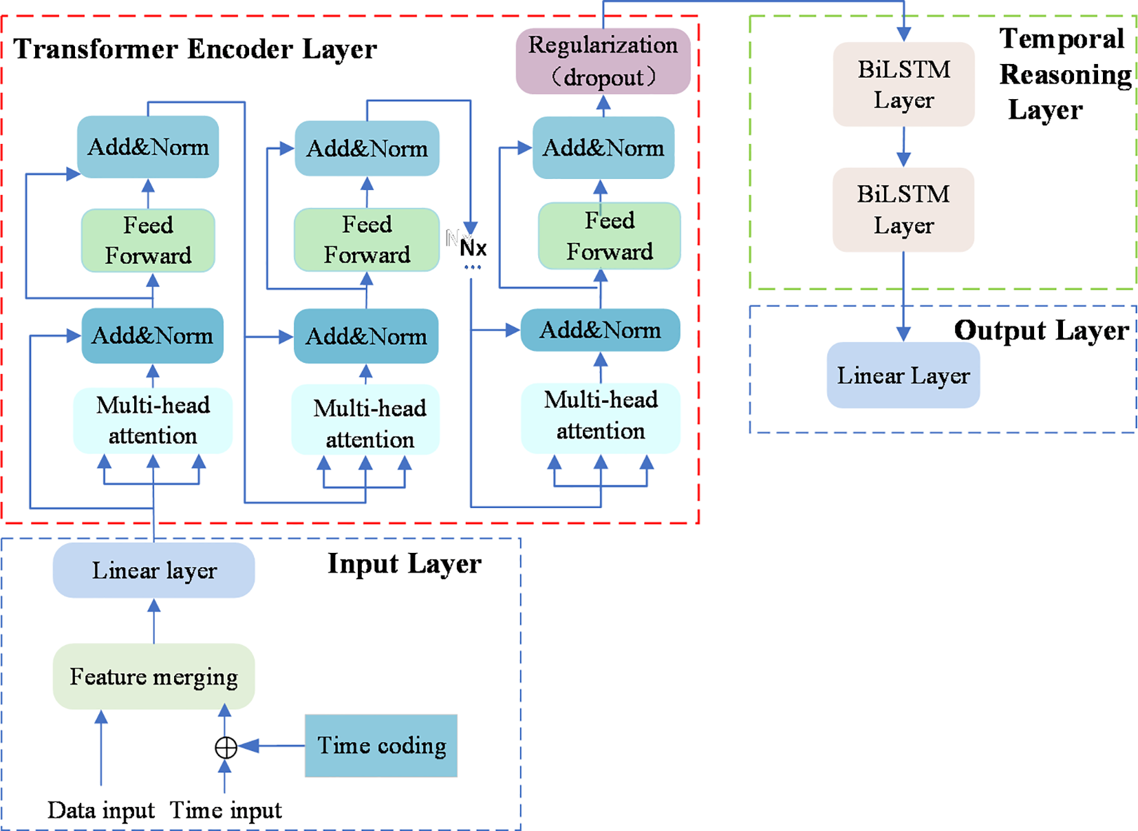
Structure of the Transformer-Encoder-BiLSTM model.
2.1.1 Input layer
The input layer of the model consists of three parts: time feature encoding, feature merging, and a linear layer. The specific structure is depicted in Figure 2. The implementation of the input layer is as follows: First, the time feature encoder processes the time column using variants of sine and cosine functions as shown in (Equations 1, 2) to encode timestamps. The sine and cosine functions transform each timestamp into a set of continuous features regarding days in the year and daily minutes, based on its temporal position within the time series. The encoding method helps the model capture the periodic and seasonal variations in time. In the process of feature merging, an expanded feature matrix is formed by concatenating the encoded time features with the original data features. Finally, the merged feature matrix is passed to a linear transformation layer, which maps the input data to the feature dimensions required by the Transformer encoder layer.
Figure 2
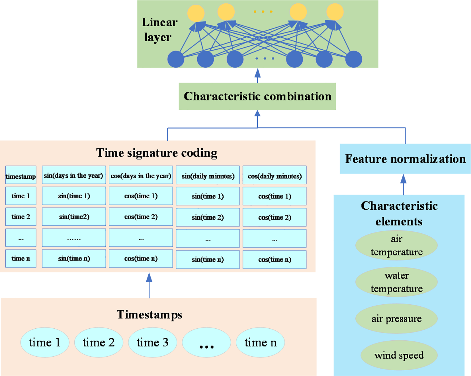
Structure of the input layer of the Transformer Encoder-BiLSTM model.
Here, PEsin refers to the sine encoding, PEcos refers to the cosine encoding, pos represents the position of the current timestamp within the sequence, i is the index of the feature dimension, d represents the feature dimension of the input data, and 104 is a constant used to adjust the frequencies of the sine and cosine functions.
The buoy-observed data of air temperature, water temperature, wind speed and air pressure are processed by Z-score standardization to ensure that the scales of all features are consistent. The equation for the standardization process is shown as (Equation 3).
In (Equation 3), X represents the original data, and μ and σ are the mean value and the standard deviation of the data respectively.
The feature fusion layer combines the time features after positional encoding with the standardized observed data features through horizontal expansion, forming an extended feature matrix. This ensures that the Transformer encoder can utilize both temporal information and data features simultaneously. The feature fusion equation is shown in (Equation 4).
In (Equation 4), is the feature element of the standardized observed data, and is the encoded time feature.
The linear layer is used to transform the fused features to fit the subsequent layers of the model. It is a fully connected layer that can perform additional linear transformations to form the final input features. The data transformation equation of the linear layer is shown in (Equation 5).
In (Equation 5), W and b are the weights and biases of the linear layer respectively, and F represents the features after feature fusion.
2.1.2 Transformer encoder layer
The encoder layer is built on the Transformer architecture and comprises multiple repeated encoder units, as demonstrated in a red dotted box in Figure 1. Each encoder layer consists of a multi-head self-attention mechanism, a feed-forward network, layer normalization, and residual connections. After the encoder layer, Dropout is applied at a specified rate to the encoded data for regularization purposes, preventing the model from overfitting during the training process.
In the encoder unit, the multi-head attention mechanism is the core component. By distributing attention across multiple heads, the model can parallelly execute single-head attention computations in multiple subspaces, extracting information. This setup allows the model to directly learn relationships between different positions in the sequence, effectively capturing complex patterns and long-distance dependencies. The single-head attention mechanism, as shown in (Equation 6), involves queries (Q), keys (K), and values (V) first being transformed through linear transformations to generate their respective weight matrices WQ, WK, and WV. The transformed Q, K, and V use a scaled dot-product operation to compute attention scores, which are then normalized through the softmax function. Multiple attention heads operate in parallel in different subspaces performing the same single-head self-attention computations, producing multiple outputs as shown in (Equation 7). The outputs from each head are concatenated and then merged into a unified output through a linear transformation layer WO, as depicted in (Equation 8). Each encoder layer also includes a feed-forward network, which independently processes the output at each position in the sequence using the equation shown in (Equation 9).
In the structure, W1 and W2 are the weight matrices of the linear layers, while b1 and b2 are the bias terms. To stabilize the training of deep networks, layer normalization and residual connections are employed as shown in (Equation 10). These techniques help maintain gradient stability and accelerate the convergence of the model.
2.1.3 BiLSTM-based temporal reasoning layer
The temporal reasoning layer consists of a bidirectional LSTM neural network (BiLSTM) which serves to enhance the model’s ability to capture long-term dependencies within the sequence to enhance time reasoning, thereby improving prediction accuracy. The structure of the BiLSTM network is shown in Figure 3, where (Figure 3A) illustrates the structure of a single LSTM cell, and (Figure 3B) depicts the overall BiLSTM network structure. Each layer is composed of a forward LSTM (running from left to right) and a backward LSTM (running from right to left).
Figure 3
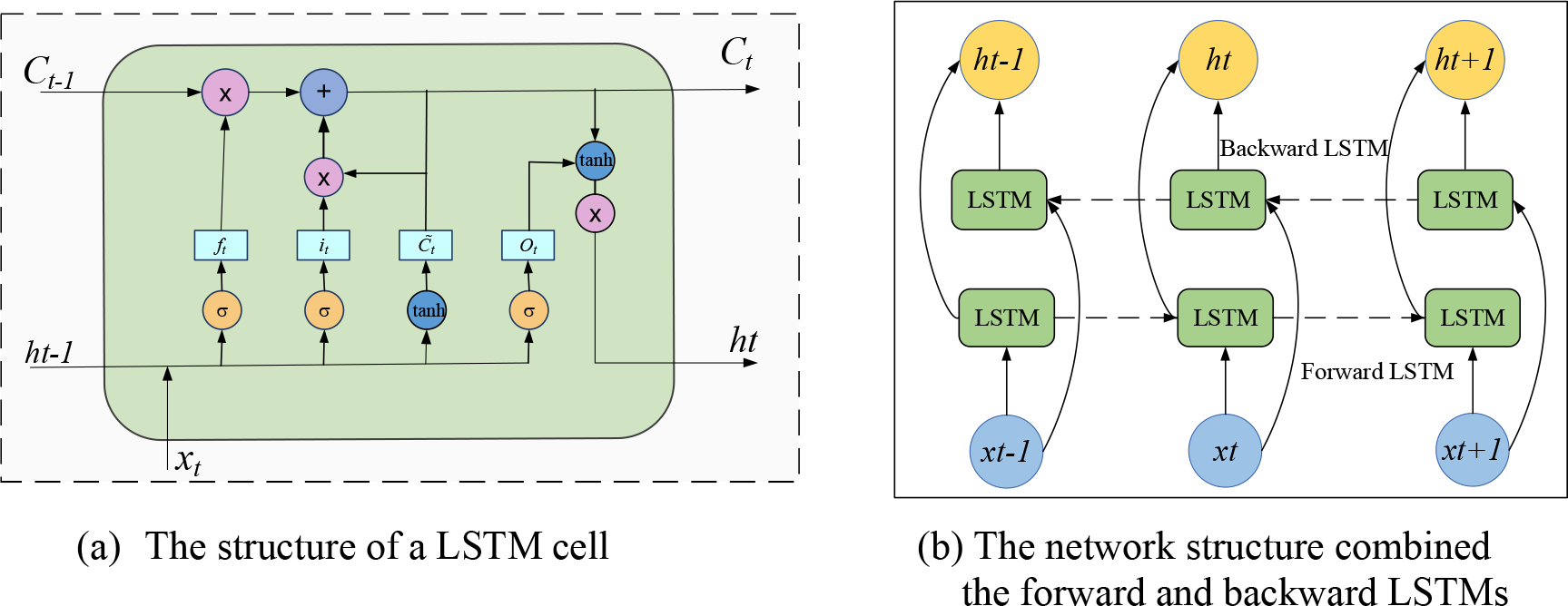
Structure of the BiLSTM network. (a) LSTM cell structure. (b) Bidirectional LSTM framework.
As shown in (Figure 3A), a single cell of the LSTM, which includes three gate structures: the forget gate (ft), the input gate (it), and the output gate (Ot). In (Figure 3A), Ct and Ct−1 represent the states of the memory units at the previous moment and the current moment respectively, ht and ht−1 represent the states of the hidden layers at the previous moment and the current moment respectively, and xt is the data input at the current moment. The forget gate ft calculates how much past information should be retained in the memory cell through an activation function sigmoid is shown in (Equation 11). The input gate it calculates how much new information enters the memory cell through an activation function sigmoid, as shown in (Equation 12). The updated value t of the cell state is obtained by performing a weighted matrix summation on the input data xt and the previous hidden state ht−1, and then passing the result through the tanh activation function, as shown in (Equation 13). The output gate Ot determines how much information is read from the memory cell. It is obtained by performing a weighted summation of the previous hidden state ht−1 and the input data xt, and then passing the result through the sigmoid activation function, as shown in (Equation 14). Finally, Ct and ht are calculated by (Equations 15, 16) respectively and are passed to the next round of calculation.
Among above equations, represents the sigmoid function. , , and are the weight matrices for the input, , and are the weight matrices related to the hidden state.
In the BiLSTM network, the forward LSTM receives the output from the Transformer encoder (depicted in Section 2.1.2) as its input, which has already integrated the global dependencies and contextual information of the sequence. Through its recursive nature, the forward LSTM enhances sensitivity to local dynamic changes in the time series. This effectively integrates and refines relevant features, and boosts its ability to parse short-term dependencies. After receiving the output from the forward BiLSTM, the backward LSTM continues to process the time series information, further synthesizing and refining the features to enhance the model’s ability to recognize complex or deep temporal patterns. The outputs of the forward and backward LSTMs are combined to integrate the complete contextual information of the time-series observation data of buoys, as shown in (Equations 17, 18, 19).
Among them, represents the output of the forward LSTM, represents the output of the backward LSTM, and H is the final output after the combination of the forward and backward LSTMs.
The bidirectional structure of the BiLSTM temporal reasoning layer enables it to integrate information from both forward and backward directions of the observation data sequence, providing the model with a more comprehensive contextual perspective and enhancing its capability to predict future sequences and interpret past states.
2.1.4 Output layer
The output layer is composed of a linear layer, with the input dimension corresponding to the hidden layer dimension of the backward LSTM, and the output dimension matching that of the target prediction variable. Its function is to ensure that the model’s output matches the dimension of the prediction target. The responsibility of the linear layer is to perform a linear transformation, mapping the output of the BiLSTM to the target space. The output of the BiLSTM is ht, which is the hidden state vector for each timestamp after processing by the backward LSTM. Therefore, the output of the linear layer can be represented as follows with Equation 20:
where, ht is the output hidden state from the second layer of the BiLSTM, W is the weight matrix of the linear layer, b is the bias term, and yt is the output of the linear layer.
The simplicity and efficiency of the linear layer make it an ideal choice for the model’s output, ensuring that the model can make accurate predictions based on the features of the time series. It serves as the final layer of the entire model and is a crucial step to generate the final prediction results that match the demanded dimension.
The Transformer-Encoder-BiLSTM model is trained using a dataset that has undergone quality control and interpolation to learn the regularities and patterns of time series data, enabling accurate predictions of buoy observed data. In the experimental phase, the predictive function of the model is used to generate temporal reference data for the test set. Finally, the reference data is used to replace observations marked as missing or fixed values and identify anomalies in the test set that were not marked with quality flag, thereby further enhancing the overall quality and reliability of the data.
2.2 Loss function, optimizer, and error metrics
The Transformer-Encoder-BiLSTM model employs Mean Squared Error (MSE) as the loss function, which calculates the average of the squared differences between the predicted values and actual values. The optimizer selected is Adam, a gradient descent algorithm that combines momentum with adaptive learning rate adjustments. The initial learning rate is set to 0.001, and it is dynamically adjusted using the ‘StepLR’ learning rate scheduler. The learning rate is multiplied by a gamma value after a certain number of training epochs, as determined by the ‘step_size’ parameter. Gamma is a multiplicative factor less than 1, used to gradually decrease the learning rate, helping the model to stabilize and converge in the later stages of training, thus avoiding overfitting.
3 Implementation of ocean moored buoy data quality control method
The workflow of the ocean moored buoy data intelligent quality control method is shown in Figure 4, which includes three stages of data cleaning, model training, and intelligent data quality control.
Figure 4
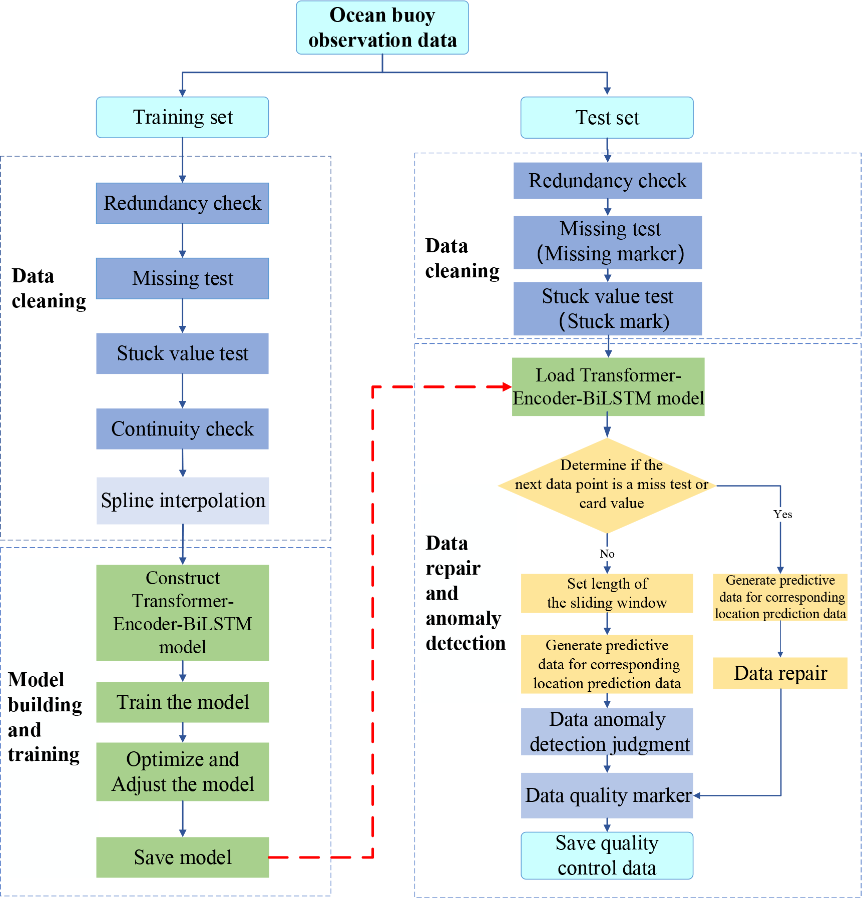
Workflow of the ocean moored buoy data intelligent quality control method.
3.1 Data cleaning
Data cleaning is performed on both training and test datasets. The steps for cleaning the training set data involve redundancy detection, missing data detection, stuck value detection, continuity detection, and spline interpolation. For the test set, data cleaning includes redundancy detection, missing data detection, and stuck value detection. The cleaned data is labeled with quality flags as shown in Table 1.
Table 1
| Quality Control Flag (Quality Code) | Meaning |
|---|---|
| Blank | Data not quality controlled |
| 1 | Correct data |
| 2 | Suspicious data |
| 3 | Missing data |
| 4 | Stuck value data |
Definition of data quality flags.
The specific data cleaning methods are as follows.
(1). Redundancy checks and missing data detection.
In the implementation process, duplicate data are identified by comparing the observation time and measured values in the buoy observation data records. If there are several records at the same observation timestamp, the average value of these records is taken as the observed value, and the redundant data are deleted. If a certain timestamp is absent, an empty record with that timestamp as the observation time will be added, and the record will be marked as missing with the symbol “3”.
(2). Stuck value detection
Stuck value detection identifies and handles fixed values in the sequence by sensor failures, transmission errors, or other technical issues. The stuck value check adopts a sliding window with a length of 6 time units, which slides along the time series. It determines whether the maximum value (Vmax) and minimum value (Vmin) of an element over a certain period meet the condition in (Equation 21). If not, the data is classified as outliers and marked with the symbol “4”. According to the China national industry standards for marine data processing1,2, the threshold values (Hh) within a sliding window for air temperature, water temperature, wind speed, and air pressure are set to 0.1, 0.1, 0.2, and 0.1 respectively.
Here, Vmax represents the maximum value of the observed data sequence, and Vmin represents the minimum value of the observed data sequence. Hh is the constant inspection parameter, which serves as the threshold for the fixed value detection.
(3). Continuity check
Gradient inspection and spike inspection are adopted to evaluate the continuity of the change values of the observation elements within a certain period of time. The specific method of the gradient inspection is as follows: Assume that the current observation value is xi, and the previous valid value adjacent to it in time or space is xi-1. It is supposed to satisfy (Equation 22). Otherwise, the observation values will be determined as suspicious.
Here, Hg is the gradient test threshold. According to the industry standards for marine data processing1,2, the Hg for air temperature and water temperature is set to 4.0, the Hg for wind speed is set to 10.0, and the Hg for air pressure is set to 1.0.
The spike inspection is based on the fact that the changes of marine observation elements within a spatial or temporal range are limited. If an observation value is significantly different from the surrounding observation values, it is determined to be abnormal. The specific method is as follows: Assume that the current data is xi, and the first correct values adjacent to it on the left and right in time or space are xi-1 and xi+1 respectively. It is supposed to satisfy (Equation 23). Otherwise, it is considered suspicious.
Here, Hjis the spike threshold. According to the China national industry standards for marine data processing1,2, the Hj for air temperature and water temperature is set to 3.0, the Hj for wind speed is set to 10.0, and the Hj for air pressure is set to 1.0.
The suspicious data detected in the processing of continuity check will be marked with the symbol “2”.
(4). Spline interpolation
For the missing data, stuck values, and suspicious data in the training set, the cubic polynomial spline interpolation method is used for filling and correction to ensure the continuity and integrity of the data during model training. The specific implementation process is as follows: First, define Si(x) as a cubic polynomial (as shown in (Equation 24)) on the specific interval [xi, xi+1]. This polynomial represents a curve between the corresponding adjacent data points xi and xi+1. Then, substitute four known data points on [xi, xi+1] into (Equation 24), and based on this, the values of ai, bi, ci, and di can be calculated. Finally, substitute the value of any point x within this interval into (Equation 24) to calculate the corresponding value, thus completing the interpolation of the data at x.
3.2 Model training and optimization
The cleaned data is fed into the Transformer-Encoder-BiLSTM time series model described in Section 3 for training. Through training and hyperparameter tuning, the model loss is reduced, and the model parameters are updated to minimize the loss function, thereby improving the model’s training effectiveness and prediction accuracy. After optimization is complete, the adjusted network model parameters are saved as a model file, which will be used for intelligent data quality control (as indicated by the red arrow in Figure 4).
During the model tuning process, the Optuna library, which is a Bayesian optimization algorithm based on a tree structure that searches for the best combination of hyperparameters through trials (Akiba et al., 2019), is used for hyperparameter optimization. The model’s hyperparameters include the batch size, the sequence length, the output dimension of input linear layer, the number of attention heads, the number of encoder layers, the number of BiLSTM hidden units, the number of BiLSTM layers, the dropout rate, the step size of the learning rate scheduler, and gamma.
One hundred optimization trials using the Optuna library were performed to minimize the mean squared error loss (MSELoss) on the validation set for determining the hyperparameter values as shown in Table 2. The optimal hyperparameters are determined according to the following process. Firstly, the value ranges were designed based on the optimal performance configurations derived from extensive preliminary experiments and performance evaluations. Subsequently, sensitivity tests were carried out on the upper and lower bounds of the parameters to ascertain which values might lead to performance degradation or overfitting. The results of these preliminary experiments disclosed that overly large or small hyperparameter values could result in a decline in model performance or induce overfitting. After that, statistical analyses were conducted on the model performance under different hyperparameter combinations, and the combinations that could significantly boost the model performance were selected. Through repeated tests, the optimal values of the hyperparameters shown in Table 2 were identified.
Table 2
| Hyperparameter Name | Value Options | Optimal Value |
|---|---|---|
| Batch size | [6, 12, 24,32] | 12 |
| Sequence Length | [3, 6, 12, 24] | 6 |
| Output dimension of input linear layer | [32, 64, 128] | 32 |
| Number of attention heads | [2, 4, 8] | 2 |
| Number of encoder layers | [1, 2, 4, 6] | 2 |
| Number of BiLSTM hidden units | [32, 64, 128, 256] | 32 |
| Number of BiLSTM layers | [1, 2, 3, 4] | 2 |
| Dropout rate | [0.1, 0.2, 0.3, 0.4, 0.5] | 0.2 |
| Step_size of learning rate scheduler | [10, 15, 20, 25, 30] | 15 |
| gamma | Range between 0 and 1 | 0.5 |
Optimal hyperparameters of the Transformer-Encoder-BiLSTM model.
3.3 Intelligent data quality control
The intelligent data quality control process consists of two modules: data repair and anomaly detection. For the test data marked as missing or fixed values, the trained Transformer-Encoder-BiLSTM model is loaded for data repair. Simultaneously, for data without quality flags, the model is executed to figure out outliers. In the procedures of data repair and anomaly detection, the Transformer-Encoder-BiLSTM model works as follows.
Firstly, the preprocessed data, which is marked with quality flags defined in Table 1, is loaded. For the missing and stuck values with the symbols ‘3 ‘ and ‘4’, the trained Transformer-Encoder-BiLSTM is executed to predict the values at corresponding timestamps and replace the original values with the predicted ones.
Secondly, anomaly detection is performed on the data entries with empty identifiers. First, load the saved Transformer-Encoder-BiLSTM model to generate the predicted data for the corresponding positions. Then, Calculate the difference between the predicted data and the original data, and use the equation outlined in (Equation 25) to determine if it is suspicious data. Data values that meet the criteria of (Equation 25) will be marked as suspicious, to be marked with a quality symbol of ‘2’; if they do not meet the criteria, they will be considered correct data, with a quality symbol of ‘1’.
Here, Vi is the i-th value of the difference sequence V between the observed data sequence A and the reference data sequence B; is the average of the difference sequence V; K is the threshold coefficient (generally set between 2 and 5) based on the confidence significance level; and σ is the standard deviation of the difference sequence V.
Finally, the system will save the quality-controlled data and conduct a comprehensive evaluation to ensure data accuracy and consistency, confirming that it meets the expected standards.
3.4 Data quality control evaluation metrics
The evaluation of quality control results is conducted using Accuracy, Precision, Recall, and F1 score. Accuracy refers to the proportion of correctly predicted samples by the model out of the total number of samples, calculated using (Equation 26); Precision refers to the proportion of samples determined as anomalies by the model that are actually anomalies, calculated using (Equation 27); Recall refers to the proportion of actual anomalies that are correctly identified as anomalies by the model, calculated using (Equation 28); and the F1 score is the harmonic mean of precision and recall, used to balance precision and recall, calculated using (Equation 29).
Here, TP stands for True Positive, indicating the number of data points that are actually anomalies and correctly detected as anomalies by the model; TN stands for True Negative, indicating the number of data points that are actually normal and correctly detected as normal by the model; FP stands for False Positive, indicating the number of data points that are actually normal but incorrectly detected as anomalies by the model; and FN stands for False Negative, indicating the number of data points that are actually anomalies but incorrectly detected as normal by the model.
4 Experiments and analysis
4.1 Hardware and software environment and experimental data
The experiments in this study were conducted on a standard desktop computer equipped with an AMD Ryzen 7 6800H processor and an RTX 3050 discrete graphics card. The software environment included the Ubuntu 20.04 operating system, the Python programming language, the neural network library PyTorch 2.2.1, the GPU computing library CUDA 12.1, and the hyperparameter optimization library Optuna.
The experimental data are sourced from Buoy No. 0199 which is deployed in the sea area near Maidao Island, Qingdao, China [the location is indicated in (Figure 5A)]. This buoy is a circular buoy with a diameter of 15 meters and is moored by three anchors [see (Figure 5B)]. The time range of the selected experimental data is from May 28, 2023, to September 8, 2023. The interval between adjacent data records is 10 minutes, and the number of data samples is 14,834. The experimental data were selected because this time period spans from late spring to early autumn. During this period, significant changes have taken place in meteorological and oceanic conditions, including the increase in temperature, fluctuations in wind speed, and changes in air pressure. Analyzing these data is of great significance and can help us better understand the impact of seasonal changes on the surrounding meteorological environment. In addition, the experimental data are derived from the actual observations of the in-situ buoys, which can reflect the real changes in the marine environment. The results of the data analysis are of even greater practical guiding significance for the R&D team of buoy equipment.
Figure 5
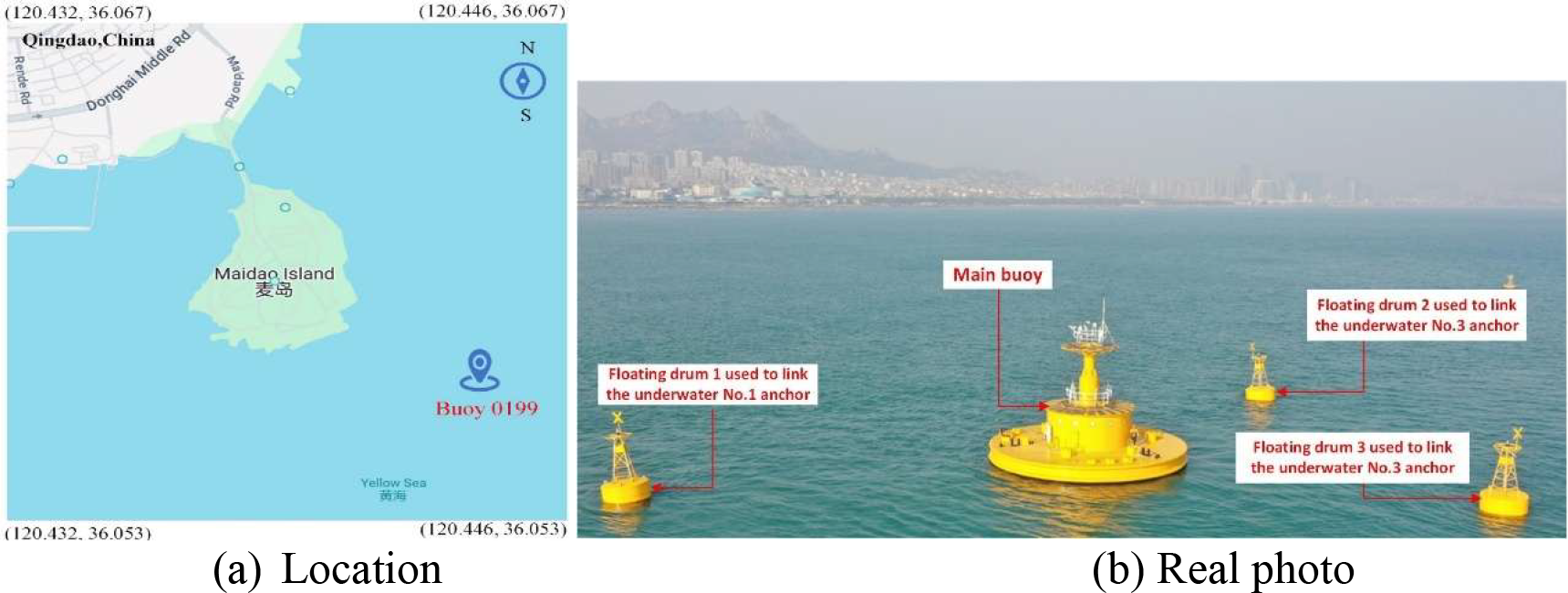
Deployment location and structure of Buoy 0199. (a) Geographical location of Buoy 0199 near Maidao Island, Qingdao, China. (b) Real-world photograph of the buoy, showing the main buoy and three floating drums connected to underwater anchors.
In the experiments, the average air temperature, water temperature, average wind speed, and average air pressure were taken as the objects of data quality control. Through the Pearson correlation coefficient test, it was found that the correlations between the air temperature and the water temperature and that between the wind speed and the air pressure are high. Additionally, data elements in the buoy observation dataset include the air temperature per minute, wind speed per minute, air pressure per minute within every 10 minutes, as well as the water temperature, average air temperature, average wind speed, and average air pressure. The input characteristic elements for the four target elements (average air temperature, water temperature, average wind speed, and average air pressure) are shown in Figure 6. The input feature elements for detecting average air temperature and water temperature include air temperature per minute within 10 minutes, average air temperature and water temperature. The input feature elements for detection average wind speed include wind speed per minute within 10 minutes, average wind speed and average air pressure. The input feature elements for detecting average air pressure include air pressure per minute within 10 minutes, average air pressure and average wind speed.
Figure 6
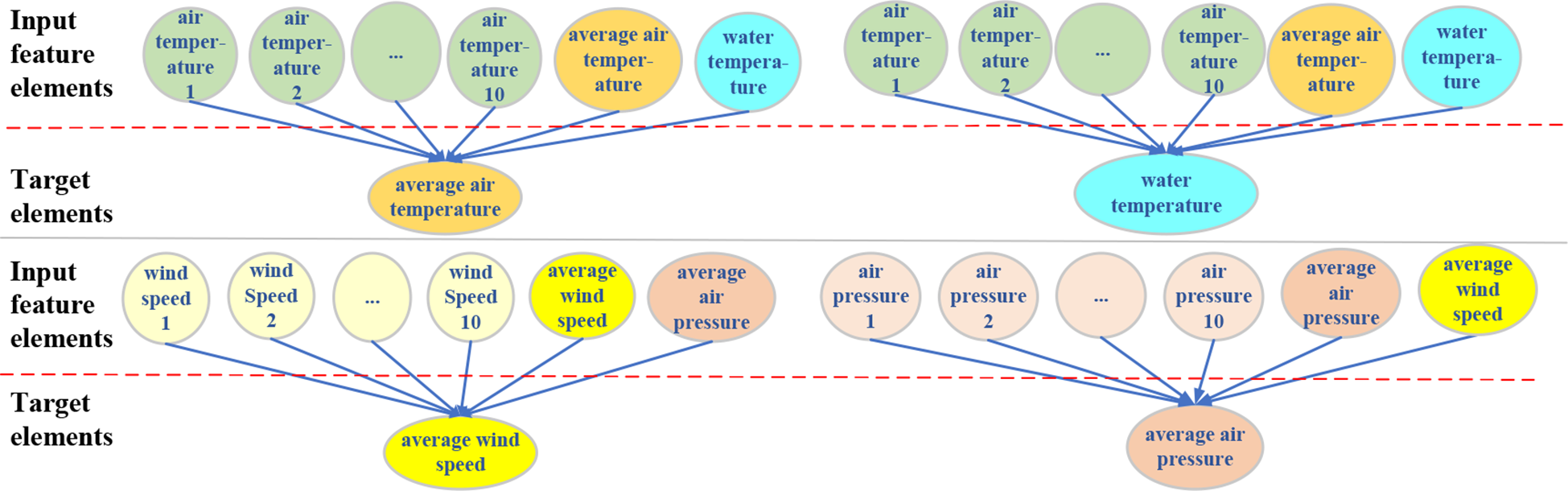
The mapping relationship between the input feature elements and the quality control target elements.
The entire experimental dataset was divided into training and test sets. The training set covers the time period from May 28, 2023, to August 6, 2023, with 10,258 data points; the test set covers the period from August 7, 2023, to September 8, 2023, with 4,576 data points. During the execution of the Transformer-encoder-BiLSTM model (described in Section 2.1.1), the variation in the dimensions of the feature data of the four target elements (average air temperature, water temperature, average wind speed, and average air pressure) in each data processing layer is shown in Table 3. The original input feature dimension is 12. After combined with encoded time feature in the procedure of feature merging, the feature dimension changes to16. After being processed by the input linear layer, the feature dimension changes to 32. Then, after passing through the Transformer-Encoder layer, deep features are extracted, and the feature dimension remains unchanged. After being processed by two layers of BiLSTM, the feature dimension reaches 64. Finally, after the processing of the linear layer, the output dimension is fixed at 1.
Table 3
| Type | Input size | Output size |
|---|---|---|
| Time coding | [batch size, sequence length,1] | [batch size, sequence length,4] |
| Fearure merging | [batch size, sequence length,12] | [batch size, sequence length,16] |
| Linear layer | batch size, sequence length,16] | [batch size, sequence length,32] |
| Transformer Encoder layer | [batch size, sequence length,32] | [batch size, sequence length,32] |
| BiLSTM Layer1 | [batch size, sequence length,32] | [batch size, sequence length,64] |
| BiLSTM Layer2 | [batch size, sequence length,64] | [batch size, sequence length,64] |
| Output layer | [batch size,64] | [batch size, 1] |
Dimensions of feature data in the Transforme-Encoder-BiLSTM network structure.
4.2 Analysis of data quality control effectiveness
4.2.1 Analysis of missing data and stuck value detection results
Missing data and stuck value detection was conducted on the four target elements (average air temperature, water temperature, average wind speed, and average air pressure) within the test set. Missing values are marked with the symbol ‘3’ and stuck values are marked with the symbol ‘4’. The visual results of missing data and stuck value detection are shown in Figure 7. In Figure 7, empty spaces indicate missing data and red dots indicate stuck values. The experimental results indicate that missing data for all four elements is concentrated within several identical time periods, with a missing rate of 8.85%. The missing data originates from common external factors, such as data transmission issues or system interruptions. For stuck value detection, threshold values for air temperature, water temperature, wind speed, and air pressure were set at 0.1, 0.1, 0.2, and 0.1 respectively. A sliding window of six time points was applied along the time series to identify stuck values. The stuck value rates for air temperature, water temperature, wind speed, and air pressure are 4.1%, 8.1%, 0.79%, and 2.69%, respectively, indicating varying degrees of stuck values among the different elements. The stuck value rate for seawater temperature is the highest, due to prolonged operation of the water temperature sensor in seawater, where it is subject to environmental interference. In contrast, the stuck value rate for wind speed is the lowest, as the wind sensor is mounted on a bracket at the top of the buoy platform, operating in open air and thus experiencing less environmental interference.
Figure 7
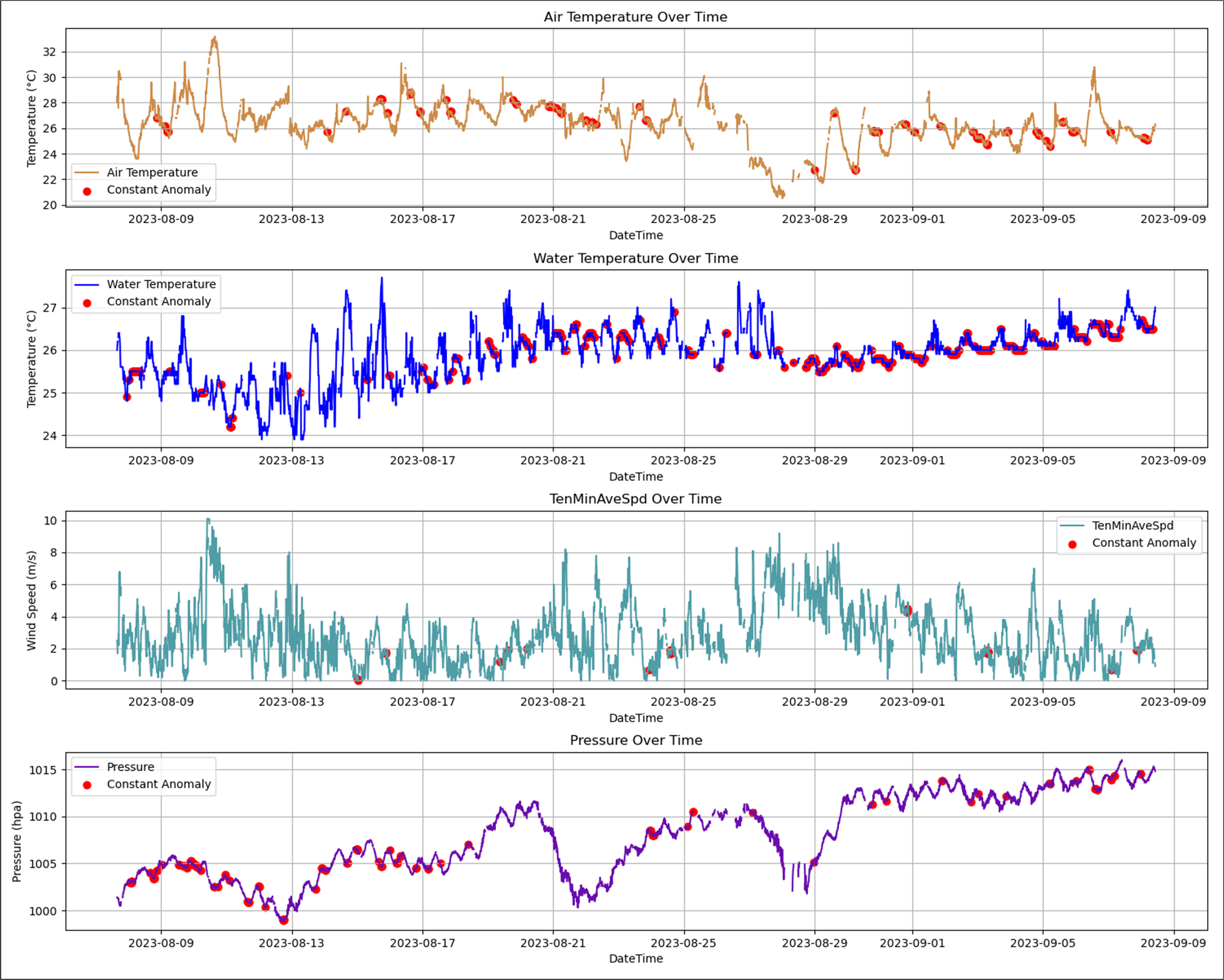
Results of missing and stuck value detection on the testing dataset.
4.2.2 Analysis of data repair results
Data repair is performed before anomaly detection to ensure data integrity. In the data repair process, the predicted values generated by the Transformer-Encoder-BiLSTM model are used to impute the missing values and replace stuck values. Figure 8 illustrates the repaired results calculated by the Transformer-Encoder-BiLSTM model for missing and stuck value data. In Figure 8, green dots represent filled values of missing data and red dots represent replaced values of stuck data. The magnified area in Figure 8 highlights the recovery of air temperature data from August 31 to September 2, 2023. It shows that the Transformer-Encoder-BiLSTM model effectively corrects missing and stuck values, providing a reliable data foundation for anomaly detection and enhancing its accuracy and effectiveness.
Figure 8
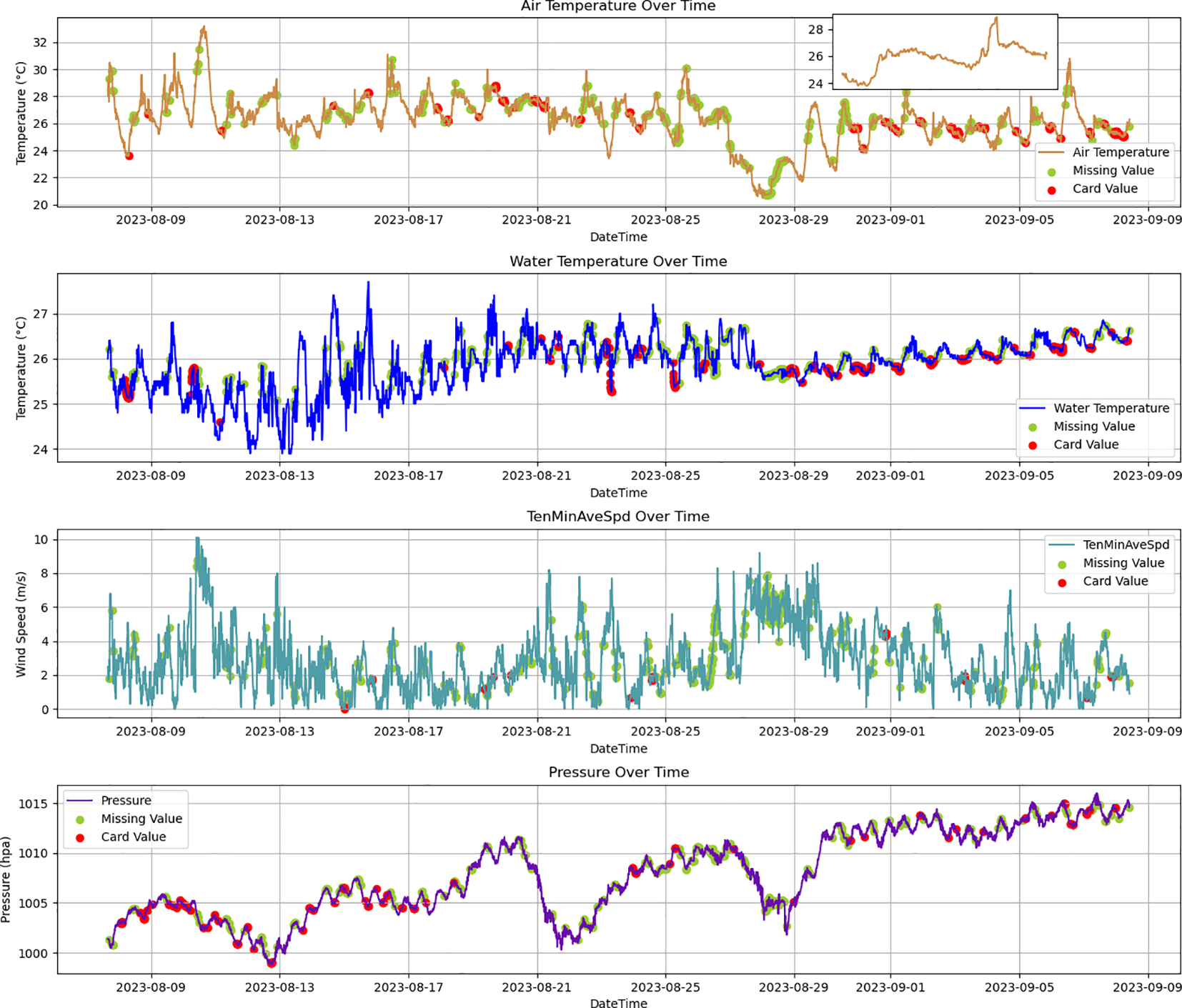
Results of repairing missing and stuck values with the Transformer-Encoder-BiLSTM model.
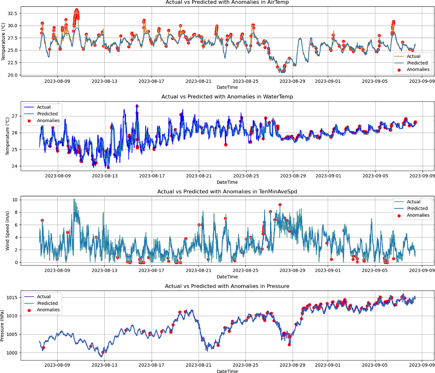
4.2.3 Analysis of anomaly detection results
The Transformer-Encoder-BiLSTM model performs further anomaly detection on data from the testing dataset that is not marked with any quality flags. Figure 9 shows the anomaly detection results based on the Transformer-Encoder-BiLSTM model, where the red dots represent outliers. The results indicate that 253, 275, 87, and 191 records are identified as anomalous for air temperature, water temperature, wind speed, and air pressure, respectively. The corresponding error rates are 6.35%, 7.69%, 2.12%, and 4.77%. It indicates that the model’s performance varies when detecting different elements, which is related to the external environment that the monitoring sensors work in. Specifically, the error rate of seawater temperature is the highest, as the water temperature sensors are installed underwater and are susceptible to fluctuations caused by waves and ocean currents, leading to increased data error rates. In contrast, the error rate of wind speed is relatively low, because the wind sensors are mounted on a 10 m high frame on top of a buoy platform, which protects them from seawater erosion, resulting in more stable data with fewer anomalies. This is consistent with the cause analysis of the stuck value detection results.
Figure 9
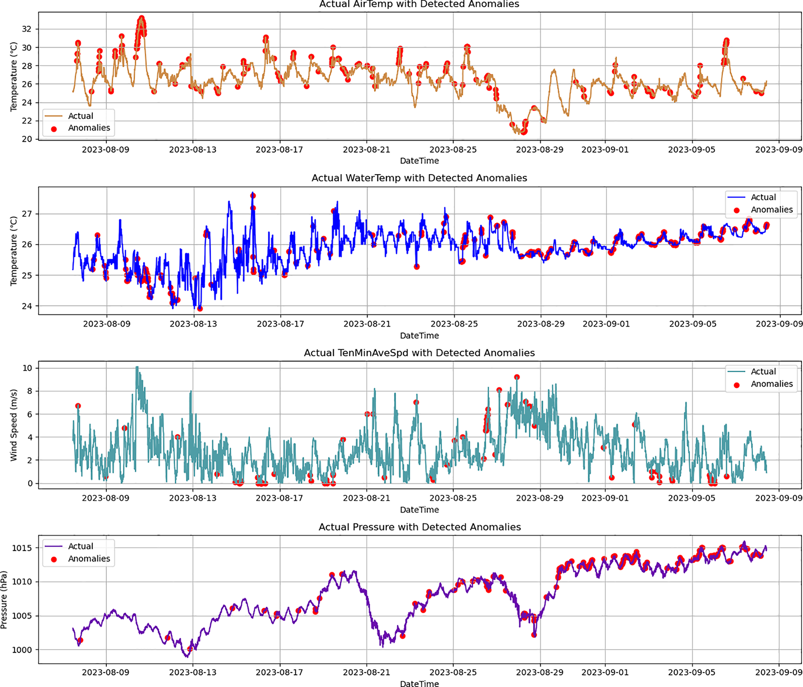
Anomaly detection results of air temperature, water temperature, wind speed, and air pressure with the Transformer-Encoder-BiLSTM model.
4.2.4 Evaluation of data quality control results
The anomaly detection results of the Transformer-Encoder-BiLSTM model are evaluated and the assessment results are shown in Table 4. From Table 4, it can be observed that the accuracy rates for the four target elements are all above 97%, demonstrating the model’s efficiency in distinguishing between correct data and anomalies. The precision rates are all above 84%, indicating the model’s accuracy in identifying anomalous data. The recall rates range between 75.61% and 85.71%, demonstrating that the model effectively identifies real anomalies with very few missed detections. The F1 scores range from 81.61% to 90.09%, further confirming the model’s high overall performance. Among the four elements, the quality control assessment for air temperature performs the best, with an F1 score of 90.09%. Overall, the Transformer-Encoder-BiLSTM model demonstrates high reliability in detecting anomalies across all four parameters: air temperature, water temperature, wind speed, and air pressure.
Table 4
| Ocean Parameters | Accuracy (%) | Precision (%) | Recall (%) | F1 (%) |
|---|---|---|---|---|
| air temperature | 98.67% | 94.86% | 85.71% | 90.09% |
| water temperature | 98.18% | 84.28%. | 78.64% | 81.61 |
| wind speed | 99.32 | 89.66% | 80.41% | 84.73% |
| air pressure | 97.82% | 92.73% | 81.41% | 86.78 |
Evaluation metrics of the Transformer-Encoder-BiLSTM model for buoy data anomaly detection.
4.2.5 Analysis of time efficiency
Using the Transformer-Encoder-BiLSTM model to carry out outlier detection for the four target elements is highly time-efficient. As shown in Figure 10, the time consumed in the four data processing stages, namely data processing, sample segmentation, model training, and model evaluation, is presented. The model training time for 10,258 data records of the training set ranges from 1,550 seconds to 1,750 seconds. Meanwhile, the model evaluation time needed for performing outlier detection on 4,576 data records of the test set is between 2.6 seconds and 3.6 seconds, suggesting a relatively fast calculation speed and its practicability in actual scenarios. By invoking the trained model, real-time outlier detection can be accomplished within 4 seconds. Experiments have verified that the Transformer-Encoder-BiLSTM model enjoys high computational efficiency.
Figure 10
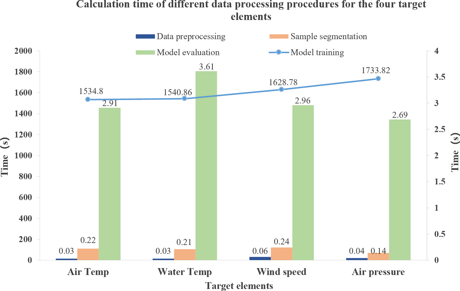
The calculation time of the Transformer-Encoder-BiLSTM model for QC of air temperature, water temperature, wind speed and air pressure.
Actually, the computational efficiency of the Transformer-Encoder-BiLSTM model will inevitably vary due to changes in on-site hardware configurations, making it difficult to ensure real-time response performance. Therefore, offline data imputation is adopted as an alternative to real-time imputation. The specific process is as follows: First, the model is pre-trained on the server every hour using the historical observation data from at least 30 days ago. Then, data anomaly detection and imputation are carried out for the data from one hour ago. Finally, the processed data is imported into the real-time data system.
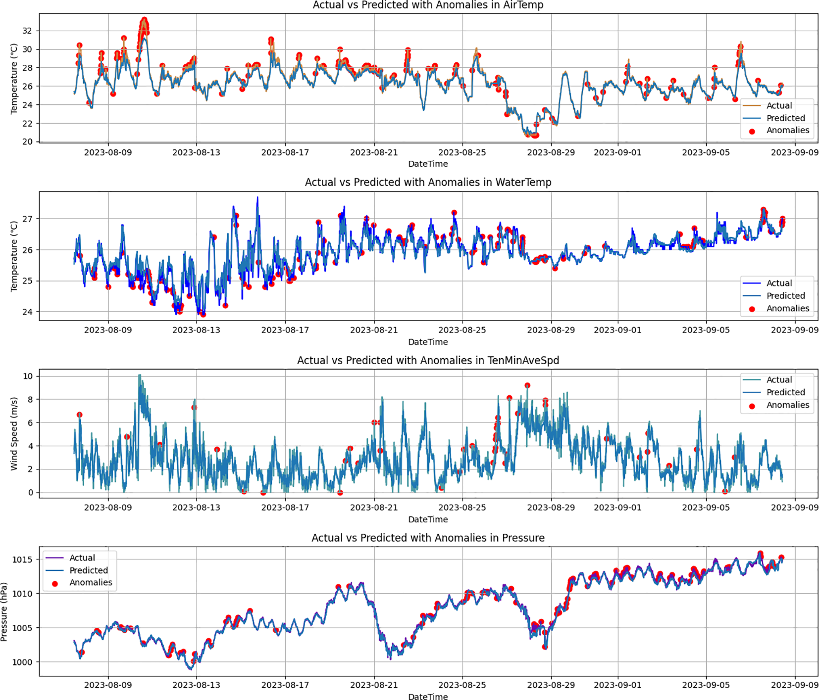
4.3 Ablation experiments
In the ablation experiments, the performance of three models—BiLSTM, Transformer-Encoder-LSTM, and Transformer-Encoder-BiLSTM—is compared. Figures 11–13 show predicted values and anomaly detection results for the BiLSTM, Transformer-LSTM, and Transformer-Encoder-BiLSTM models, respectively. The different detection methods revealed their sensitivity and ability to identify anomalies in temperature, water temperature, wind speed, and air pressure. For the BiLSTM model, the number of detected suspicious data points is as follows: 272 for air temperature, 263 for water temperature, 74 for wind speed, and 196 for air pressure. The Transformer-LSTM model detected slightly more suspicious data points: 291 for air temperature, 270 for water temperature, 85 for wind speed, and 181 for air pressure. In contrast, the Transformer-Encoder-BiLSTM model, which integrates both the Transformer encoder and BiLSTM, identified 253 suspicious data points for air temperature, 275 for water temperature, 87 for wind speed, and 191 for air pressure. These time series models demonstrate high sensitivity in identifying anomalous data. Further quality evaluation of these anomaly detection methods was conducted, with detailed results shown in Table 5. Experimental results indicate that the Transformer-Encoder-BiLSTM model outperforms the other two models in accuracy, precision, recall, and F1 score for detecting anomalies in air temperature, water temperature, wind speed, and air pressure, highlighting its superior anomaly detection capability.
Figure 11
Predicted values and anomaly points got using the BiLSTM model.
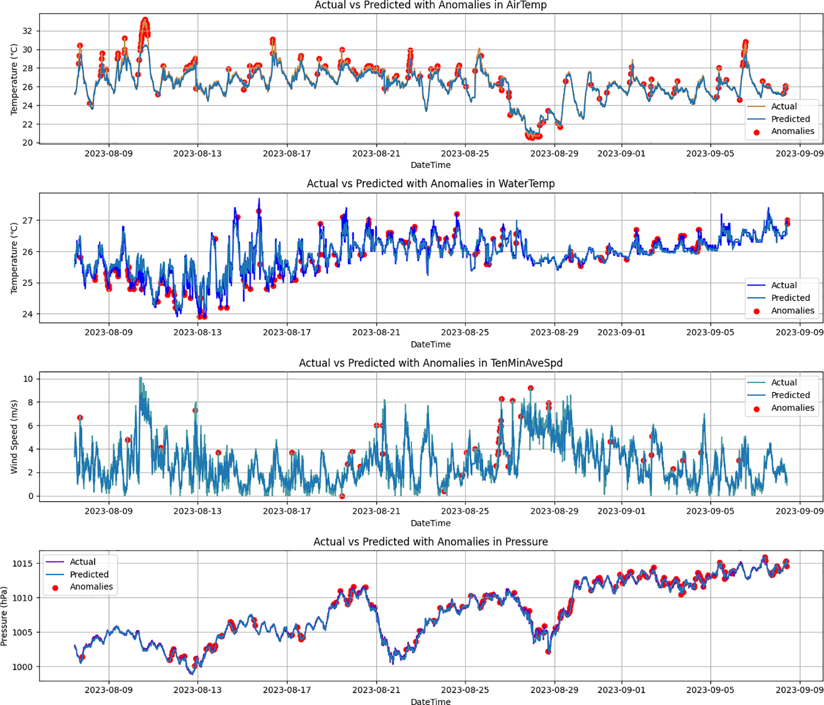
Figure 12
Predicted values and anomaly points got using the Transformer-Encoder-LSTM model.
Figure 13
Predicted values and anomaly points got using the Transformer-Encoder-BiLSTM model.
Table 5
| Detection | Accuracy | Precision | Recall | F1 |
|---|---|---|---|---|
| BiLSTM | 97.30% | 84.60% | 78.46% | 80.20% |
| Transformer-Encoder-LSTM | 98.35% | 89.20% | 81.60% | 85.42% |
| Transformer-Encoder-BiLSTM | 98.50% | 90.38% | 81.64% | 85.80% |
Evaluation metrics of the BiLSTM model, the Transformer-Encoder-LSTM model and the Transformer-Encoder-BiLSTM model for detecting anomalies.
Further comparison of the three models in terms of MAE, MSE, RMSE, and R² metrics is provided in Table 6. The results show that the proposed Transformer-Encoder-BiLSTM model, which combines the efficient data encoding capabilities of the Transformer encoder with the strong temporal information processing abilities of the bidirectional LSTM, demonstrates excellent model performance. Specifically, this model achieves an MAE of 0.122, MSE of 0.032, RMSE of 0.180, and an R² score of 0.916, outperforming the other two models in all metrics.
Table 6
| Model | MAE | MSE | RMSE | R2 |
|---|---|---|---|---|
| BiLSTM | 0.208 | 0.062 | 0.249 | 0.838 |
| Transformer-Encoder-LSTM | 0.137 | 0.038 | 0.197 | 0.898 |
| Transformer-Encoder-BiLSTM | 0.122 | 0.032 | 0.180 | 0.916 |
Performance comparison of the BiLSTM model, the Transformer-Encoder-LSTM model and the Transformer-Encoder-BiLSTM model.
The above results of ablation experiments indicate that incorporating the Transformer encoder and the bidirectional LSTM to build the Transformer-Encoder-BiLSTM model significantly enhances the performance of anomaly detection. The Transformer encoder layer effectively captured the complex dependencies and nonlinear features in the ocean observation data. The bidirectional LSTM further strengthened the model’s capacity to capture contextual information in the time series. This enhanced the model’s ability to understand long-term trends and, ultimately optimized the model’s overall predictive performance for detecting anomalous data.
4.4 Comparative experiments
The QC method using the Transformer-Encoder-BiLSTM model was compared with traditional ocean data QC methods, namely Grubbs’ test and the 3σ criterion, as well as the state-of-the-art AI models, such as the Seasonal and Trend decomposition using Loess and LSTM model (STL-LSTM) (Feng et al., 2021) and the CNN-BiGRU-Attention model (Song et al., 2024), with detailed results shown in Table 7. The experiments indicate that traditional methods have lower recall rates, making them prone to missing anomalous data, resulting in lower overall performance (F1 score) compared to deep learning models. Among all metrics, the Transformer-Encoder-BiLSTM model performed the best, particularly excelling in precision and F1 score, demonstrating its ability to effectively balance accuracy and recall in detecting anomalous data, and showcasing the strongest overall performance.
Table 7
| Detection | Accuracy | Precision | Recall | F1 |
|---|---|---|---|---|
| Grubbs Test | 94.52% | 82.29% | 60.20% | 81.20% |
| 3σ Criterion | 95.63% | 82.86% | 60.10% | 81.58% |
| CNN-BiGRU-Attention | 96.63% | 84.28% | 75.48% | 82.61% |
| STL-LSTM | 97.50% | 88.69% | 80.52% | 84.50% |
| Transformer-Encoder-BiLSTM | 98.50% | 90.38% | 81.64% | 85.80% |
Evaluation metrics of Grubbs Test, 3σ Criterion, the CNN-BiGRU-Attention model, the STL-LSTM model and the Transformer-Encoder-BiLSTM model for Buoy Data Detection.
The Transformer-Encoder-BiLSTM model was compared with the CNN-BiGRU-Attention model and the STL-LSTM model in terms of four performance indicators: MAE, MSE, RMSE, and R2. The results are shown in Table 8, which indicates that the Transformer-Encoder-BiLSTM model proposed in this paper has high performance.
Table 8
| Model | MAE | MSE | RMSE | R2 |
|---|---|---|---|---|
| CNN-BiGRU-Attention | 0.228 | 0.068 | 0.261 | 0.903 |
| STL-LSTM | 0.330 | 0.036 | 0.190 | 0.890 |
| Transformer-Encoder-BiLSTM | 0.122 | 0.032 | 0.180 | 0.916 |
Performance comparison the CNN-BiGRU-Attention model, the STL-LSTM model and the Transformer-Encoder-BiLSTM model.
4.5 Robustness verification
The robustness verification of outlier detection was additionally conducted on the datasets of Buoy No. 0234, situated in Jiaozhou Bay, China, and Buoy No. 0235, which is located in the Bohai Strait. The performance comparison of the Transformer-Encoder-BiLSTM model for data outlier detection of Buoy No. 0199, Buoy No. 0234, and Buoy No. 0235 is presented in Table 9. It can be noted that the MAE of the data is below 0.22, the MSE is below 0.12, the RMSE is below 0.34, and the R2 value is above 85%. This suggests that the Transformer-Encoder-BiLSTM data quality control model proposed in this paper possesses good robustness and is able to detect outliers in the observed data from various buoy stations.
Table 9
| Buoy No. | MAE | MSE | RMSE | R2 |
|---|---|---|---|---|
| 0234 | 0.208 | 0.106 | 0.254 | 0.862 |
| 0235 | 0.211 | 0.114 | 0.338 | 0.858 |
| 0199 | 0.122 | 0.032 | 0.180 | 0.916 |
Performance comparison of the Transformer-Encoder-BiLSTM model on dataset of three buoys.
5 Conclusion and discussion
The long-term and continuous observations provided by moored buoys are of immense scientific value, but anomalies and data gaps disrupt this continuity and diminish the data’s applicational value. This article innovatively establishes an intelligent buoy data QC method through the organic fusion of the Transformer encoder and a BiLSTM time series analysis model, named Transformer-Encoder-BiLSTM. The buoy data QC method based on the Transformer-Encoder-BiLSTM model overcomes the defects of traditional QC methods, which can only identify gross errors and are unable to automatically detect outliers. The Transformer-Encoder-BiLSTM model demonstrates strong sensitivity to complex time-series buoy data for detecting subtle differences in nonlinearity and achieves high recall rates in anomaly detection. The innovation of the proposed data QC method is manifested as follows: 1) By taking advantage of the Transformer model, the positional data of each observation point is calculated through the self-attention mechanism. This enables the method to capture the long-distance correlations existing in the time series. Moreover, it can automatically learn the importance weights among the data of different time points in the time series data and encode feature data, which efficiently reflects the inherent temporal correlations within the data. It also boosts robustness to noisy data and improves the generalization ability of the Transformer-Encoder-BiLSTM model. 2) Employing BiLSTM enables the modeling of elements in each dimension of the encoded feature sequence from both the forward and backward directions, realizing temporal reasoning, and enhancing the accuracy of data prediction.
Ablation experiments, along with a large number of comparative experiments, and robustness experiments have been conducted to verify the effectiveness, robustness, and generalization ability of the Transformer-Encoder-BiLSTM model. Experiments have demonstrated that the model attains high performance. Specifically, for the four target elements (average air temperature, water temperature, average wind speed and average air pressure) of Buoy No. 0199 in Maidao Island, Qingdao, China, it has an R² exceeding 0.9, a quality control accuracy higher than 97%, precision and recall above 84%, and F1 scores ranging from 81.61% to 90.09%. The performance of the Transformer-Encoder-BiLSTM model has been proven to be superior to that of STL-LSTM and CNN-BiGRU-Attention. When the model was used to detect outliers in the data of another two buoys (No. 0234 and No. 0235), it also achieved good results, with the R2 values being greater than 85%, which demonstrates that the Transformer-Encoder-BiLSTM model has high robustness.
This article focuses on addressing the key technical issues during the development of marine buoy equipment. Great efforts are made to detect outliers, impute missing data, and repair stuck values and abnormal data in the observation dataset collected by our own in-situ buoy devices to enhance the quality and reliability of the data. In the future, public datasets like those in SeaDataNet will be used for model experimental verification. Additionally, future research will focus on optimizing the Transformer-Encoder-BiLSTM model for spatiotemporal quality control of other ocean buoy data elements, considering multi-station data quality across different observation sites, elements, and scales, so as to improve the robustness and generalization ability of the model. We also plan to study other neural network models, such as the spectral temporal convolutional neural network, for the high-precision QC of marine buoy data. In conclusion, this article reports an effective attempt at addressing issues of buoy data QC by leveraging the state-of-the-art neural networks, namely the Transformer-Encoder-BiLSTM. It holds great potential for establishing a comprehensive intelligent quality control method for ocean-moored buoy data.
Statements
Data availability statement
The original contributions presented in the study are included in the article/supplementary material, further inquiries can be directed to the corresponding author/s.
Author contributions
MS: Writing – original draft, Writing – review & editing, Conceptualization, Methodology, Supervision. SG: Writing – original draft, Writing – review & editing, Data curation, Investigation, Methodology, Software, Validation, Visualization. SL: Writing – original draft, Writing – review & editing, Conceptualization, Formal analysis, Funding acquisition, Resources. YX: Writing – original draft, Writing – review & editing, Conceptualization, Methodology, Project administration. SC: Writing – original draft, Writing – review & editing, Conceptualization, Formal analysis, Project administration. WL: Writing – original draft, Writing – review & editing, Software, Validation. JZ: Writing – review & editing, Resources, Data curation. KZ: Writing – original draft, Writing – review & editing, Conceptualization, Resources. XF: Formal analysis, Funding acquisition, Methodology, Project administration, Writing – original draft, Writing – review & editing.
Funding
The author(s) declare that financial support was received for the research and/or publication of this article. This work is supported by the Taishan Industrial Program Key R&D Program of Shandong Province, China (2023ZLYS01), the project “Research on intelligent analysis method of data reliability of Marine data buoy based on machine learning” supported by Qingdao Natural Science Foundation (23-2-1-159-zyyd-jch) and Qilu University of Technology (Shandong Academy of Sciences) Major innovation project of science, education and production integration pilot project (2023JBZ02). This work is also supported by Laoshan Laboratory.
Conflict of interest
The authors declare that the research was conducted in the absence of any commercial or financial relationships that could be construed as a potential conflict of interest.
Generative AI statement
The author(s) declare that no Generative AI was used in the creation of this manuscript.
Publisher’s note
All claims expressed in this article are solely those of the authors and do not necessarily represent those of their affiliated organizations, or those of the publisher, the editors and the reviewers. Any product that may be evaluated in this article, or claim that may be made by its manufacturer, is not guaranteed or endorsed by the publisher.
References
1
Akiba T. Sano S. Yanase T. Ohta T. Koyama M. (2019). Optuna: A next-generation hyperparameter optimization framework. In: Proceedings of the 25th ACM SIGKDD International Conference on Knowledge Discovery & Data Mining (KDD '19), August 4–8, 2019, Anchorage, AK, USA. New York, NY: Association for Computing Machinery (ACM), pp. 2623–2631. doi: 10.1145/3292500.3330701
2
Bi J. Zhang L. Yuan H. Zhang J. (2023). Multi-indicator water quality prediction with attention-assisted bidirectional LSTM and encoder-decoder. Inf. Sci.625, 65–80. doi: 10.1016/j.ins.2022.12.091
3
Chen Y. Cai C. Cao L. Zhang D. Kuang L. Peng Y. et al . (2024). WindFix: Harnessing the power of self-supervised learning for versatile imputation of offshore wind speed time series. Energy287. doi: 10.1016/j.energy.2023.128995
4
Cowley R. Killick R. E. Boyer T. Gouretski V. Reseghetti F. Kizu S. et al . (2021). International quality-controlled ocean database (IQuOD) v0.1: the temperature uncertainty specification. Front. Mar. Sci.8. doi: 10.3389/fmars.2021.689695
5
Cummings J. A. (2011). “Ocean data quality control,” in Operational oceanography in the 21st century. Dordrecht, Netherlands: Springer, pp. 91–121. doi: 10.1007/978-94-007-0327-8_4
6
Feng J. Huang L. Song R. Huang H. (2021). An improved STL-LSTMModel for daily bus passenger flowPrediction during the COVID-19Pandemic. Sensors21, 5950. doi: 10.3390/s21175950
7
Good S. Mills B. Boyer T. Bringas F. Castelão G. Cowley R. et al . (2023). Benchmarking of automatic quality control checks for ocean temperature profiles and recommendations for optimal sets. Front. Mar. Sci.9. doi: 10.3389/fmars.2022.1075510
8
Hochreiter S. Schmidhuber J. (1997). Long short-term memory. Neural Comput.9, 1735–1780. doi: 10.1162/neco.1997.9.8.1735
9
Iafolla L. Fiorenza E. Chiappini M. Carmisciano C. Iafolla V. A. (2022). Sea wave data reconstruction using micro-seismic measurements and machine learning methods. Front. Mar. Sci.9. doi: 10.3389/fmars.2022.798167
10
Ingleby B. Huddleston M. (2007). Quality control of ocean temperature and salinity profiles — Historical and real-time data. J. Mar. Syst.65, 158–175. doi: 10.1016/j.jmarsys.2005.11.019
11
Jörges C. Berkenbrink C. Stumpe B. (2021). Prediction and reconstruction of ocean wave heights based on bathymetric data using LSTM neural networks. Ocean Eng.232. doi: 10.1016/j.oceaneng.2021.109046
12
Li H. Peng Q. Mou X. Wang Y. Zeng Z. Bashir M. F. (2023). Abstractive financial news summarization via transformer-biLSTM encoder and graph attention-based decoder. IEEE/ACM Trans. Audio Speech Lang. Process.31, 3190–3205. doi: 10.1109/taslp.2023.3304473
13
Liu S. Song M. Chen S. Fu X. Zheng S. Hu W. et al . (2023). An intelligent modeling framework to optimize the spatial layout of ocean moored buoy observing networks. Front. Mar. Sci.10. doi: 10.3389/fmars.2023.1134418
14
Ma M. Han L. Zhou C. (2023). BTAD: A binary transformer deep neural network model for anomaly detection in multivariate time series data. Advanced Eng. Inf.56, 101949. doi: 10.1016/j.aei.2023.101949
15
Martínez-Osuna J. F. Ocampo-Torres F. J. Gutiérrez-Loza L. Valenzuela E. Castro A. Alcaraz R. et al . (2021). Coastal buoy data acquisition and telemetry system for monitoring oceanographic and meteorological variables in the Gulf of Mexico. Measurement183, 109841. doi: 10.1016/j.measurement.2021.109841
16
Mieruch S. Demirel S. Simoncelli S. Schlitzer R. Seitz S. (2021). SalaciaML: A deep learning approach for supporting ocean data quality control. Front. Mar. Sci.8, 611742. doi: 10.3389/fmars.2021.611742
17
Ono S. Matsuyama H. Fukui K.-I. Hosoda S. (2015). A preliminary study on quality control of oceanic observation data by machine learning methods. In: Proceedings of the 18th Asia Pacific Symposium on Intelligent and Evolutionary Systems (IES 2014), Volume 1, November 10–12, 2014, Singapore. Springer: Cham, pp. 679–693. doi: 10.1007/978-3-319-27146-0_53
18
Palmer M. D. Boyer T. Cowley R. Kizu S. Reseghetti F. Suzuki T. et al . (2018). An algorithm for classifying unknown expendable bathythermograph (XBT) instruments based on existing metadata. J. Atmospheric Oceanic Technol.35, 429–440. doi: 10.1175/jtech-d-17-0129.1
19
Qian C. Liu A. Huang R. Liu Q. Xu W. Zhong S. et al . (2019). Quality control of marine big data—a case study of real-time observation station data in Qingdao. J. Oceanology Limnology37, 1983–1993. doi: 10.1007/s00343-019-8258-y
20
Rapizo H. Babanin A. V. Schulz E. Hemer M. A. Durrant T. H. (2015). Observation of wind-waves from a moored buoy in the Southern Ocean. Ocean Dynamics65, 1275–1288. doi: 10.1007/s10236-015-0873-3
21
Schaap D. M. A. Lowry R. K. (2010). SeaDataNet – Pan-European infrastructure for marine and ocean data management: unified access to distributed data sets. Int. J. Digital Earth3, 50–69. doi: 10.1080/17538941003660974
22
Song M. Hu W. Liu S. Chen S. Fu X. Zhang J. et al . (2024). Developing an artificial intelligence based method for predicting the trajectory of surface drifting buoys using a hybrid multi-layer neural network model. J. Mar. Sci. Eng.12, 958. doi: 10.3390/jmse12060958
23
Tan Z. Zhang B. Wu X. Dong M. Cheng L. (2021). Quality control for ocean observations: From present to future. Sci. China Earth Sci.65, 215–233. doi: 10.1007/s11430-021-9846-7
24
Tuli S. Casale G. Jennings N. R. (2022). Tranad: Deep transformer networks for anomaly detection in multivariate time series data (arXiv preprint). arXiv:2201.07284. https://arxiv.org/abs/2201.07284.
25
Vaswani A. Shazeer N. Parmar N. Uszkoreit J. Jones L. Gomez A. N. et al . (2017). Attention is all you need. In: Proceedings of the 31st International Conference on Neural Information Processing Systems (NeurIPS 2017), December 4–9, 2017, Long Beach, CA, USA. Curran Associates, Inc., Red Hook, NY, USA, pp. 5998–6008.
26
Vieira F. Cavalcante G. Campos E. Taveira-Pinto F. (2020). A methodology for data gap filling in wave records using Artificial Neural Networks. Appl. Ocean Res.98, 102109. doi: 10.1016/j.apor.2020.102109
27
von Schuckmann K. Le Traon P.-Y. Alvarez-Fanjul E. Axell L. Balmaseda M. Breivik L.-A. et al . (2017). The copernicus marine environment monitoring service ocean state report. J. Operational Oceanography9, s235–s320. doi: 10.1080/1755876x.2016.1273446
28
Wang S. (2023). A stock price prediction method based on biLSTM and improved transformer. IEEE Access11, 104211–104223. doi: 10.1109/access.2023.3296308
29
Wang X. Pi D. Zhang X. Liu H. Guo C. (2022). Variational transformer-based anomaly detection approach for multivariate time series. Measurement191, 110791. doi: 10.1016/j.measurement.2022.110791
30
Wang J. Wang Z. Wang Y. Liu S. Li Y. (2016). Current situation and trend of marine data buoy and monitoring network technology of China. Acta Oceanologica Sin.35, 1–10. doi: 10.1007/s13131-016-0815-z
31
Wen J. Yang J. Jiang B. Song H. Wang H. (2021). Big data driven marine environment information forecasting: A time series prediction network. IEEE Trans. Fuzzy Syst.29, 4–18. doi: 10.1109/tfuzz.2020.3012393
32
Wen Q. Zhou T. Zhang C. Chen W. Ma Z. Yan J. et al . (2022). Transformers in time series: A survey (arXiv preprint). arXiv:2202.07125. https://arxiv.org/abs/2202.07125.
33
Wong A. P. S. Wijffels S. E. Riser S. C. Pouliquen S. Hosoda S. Roemmich D. et al . (2020). Argo data 1999–2019: two million temperature-salinity profiles and subsurface velocity observations from a global array of profiling floats. Front. Mar. Sci.7. doi: 10.3389/fmars.2020.00700
34
Xie J. Jiang H. Song W. Yang J. (2023). A novel quality control method of time-series ocean wave observation data combining deep-learning prediction and statistical analysis. J. Sea Res.195, 102439. doi: 10.1016/j.seares.2023.102439
35
Yao J. Wu W. Li S. (2022). Anomaly detection model of mooring system based on LSTM PCA method. Ocean Eng.254, 111350. doi: 10.1016/j.oceaneng.2022.111350
36
Zhao Z. Chen Y. Liu J. Cheng Y. Tang C. Yao C. (2023). Evaluation of operating state for smart electricity meters based on transformer–encoder–biLSTM. IEEE Trans. Ind. Inf.19, 2409–2420. doi: 10.1109/tii.2022.3172182
37
Zhou Y. Qin R. Xu H. Sadiq S. Yu Y. (2018). A data quality control method for seafloor observatories: the application of observed time series data in the east China sea. Sensors (Basel)18 (8), 2628. doi: 10.3390/s18082628
Summary
Keywords
ocean moored buoy, data quality control, transformer encoder, BiLSTM, anomaly detection, data correction
Citation
Song M, Gao S, Liu S, Xu Y, Chen S, Zhang J, Li W, Zhang K and Fu X (2025) Intelligent quality control method for marine buoy data based on transformer encoder and BiLSTM. Front. Mar. Sci. 12:1528587. doi: 10.3389/fmars.2025.1528587
Received
01 December 2024
Accepted
07 April 2025
Published
30 April 2025
Volume
12 - 2025
Edited by
Zhibin Yu, Ocean University of China, China
Reviewed by
Yaofeng Xie, Ocean University of China, China
Liye Zhang, Shandong University of Science and Technology, China
Wen Zhang, National University of Defense Technology, China
Zhichao Cai, East China Jiaotong University, China
Updates
Copyright
© 2025 Song, Gao, Liu, Xu, Chen, Zhang, Li, Zhang and Fu.
This is an open-access article distributed under the terms of the Creative Commons Attribution License (CC BY). The use, distribution or reproduction in other forums is permitted, provided the original author(s) and the copyright owner(s) are credited and that the original publication in this journal is cited, in accordance with accepted academic practice. No use, distribution or reproduction is permitted which does not comply with these terms.
*Correspondence: Shixuan Liu, lsx@sdioi.com; Yuzhe Xu, cosmo.xu@outlook.com
Disclaimer
All claims expressed in this article are solely those of the authors and do not necessarily represent those of their affiliated organizations, or those of the publisher, the editors and the reviewers. Any product that may be evaluated in this article or claim that may be made by its manufacturer is not guaranteed or endorsed by the publisher.