Abstract
Several global and regional initiatives exist to increase the proportion of seafloor mapped by direct measurements, brought together through international collaborations, of which the Nippon Foundation-GEBCO Seabed 2030 Project is perhaps the most well-known. Nearly halfway into the United Nations Decade of Ocean Science for Sustainable Development, we used publicly available bathymetric and type-identifier datasets from the General Bathymetric Chart of the Oceans (GEBCO) to systematically evaluate progress in the global seafloor mapping effort between 2019 and 2024. We explore each major ocean basin and sea, exclusive economic zones (EEZs), and different depth zones. Proportionally, the North Atlantic (NAO) and North Pacific (NPO) have the highest mapping coverage, with over a third of each ocean mapped by the end of 2024. Nearly 30% of the seafloor in the Arctic Ocean (AO), South Atlantic Ocean (SAO), and Southern Ocean (SO) has been mapped by 2024. In contrast, the Indian Ocean (IO) remains the least mapped, with only 17.5% coverage. When considering mapping coverage by depth zones, approximately one-quarter of shallow areas (0–200 m) and the abyssal zone (3000–6000 m) have been mapped, comprising 6.3% and 68.4% of the global mapped seafloor area, respectively. Nearly 40% of seafloor in the upper (200–1000 m) and lower (1000–3000 m) bathyal zones has been mapped, corresponding to 5.6% and 17.7% of the global total mapped area. Although, the hadal zone (>6000 m) makes up only 1.0% of the global seafloor, it has the highest (55.6%) proportional mapping coverage, comprising up to 2.0% of global mapping effort. Evaluation of mapping coverage by sovereign states shows that progress is strongly influenced by EEZ size, economic status and the presence of offshore resources. This study reveals the uneven mapping efforts worldwide and suggests that more focus should be given to the two polar oceans, IO, and Southern Hemisphere in general, as well as the EEZs of African and Asian states, to reach the average global coverage. With the current average rate of new map generation of ∼3.2% of total seafloor area annually, we predict that the global seafloor could be mapped in approximately 20 years. Analysis of the seafloor mapping efforts in different depth zones of ocean basins, EEZs, and ABNJ provide future priority areas of exploration for the Seabed 2030 initiative.
Introduction
The ocean, covering 71% (∼362 million km2) of the surface of our planet, plays a fundamental role in sustaining life, controlling climate and facilitating commerce, representing a vast source of resources and economic wealth (Worm et al., 2006; Anderson and Peters, 2016; Mayer et al., 2018; Wölfl et al., 2019; Frazão Santos et al., 2020). It provides the basis of many existing and emerging human activities including navigation (commercial and defence), food resources, renewable energy, and marine resource management, among many others (Visbeck et al., 2014; Halpern et al., 2019; Ryabinin et al., 2019). Water depth and seafloor morphology influence environmental factors including light penetration and photosynthesis, sedimentation, current movements, and water column stratification, which govern species distribution patterns and productivity in the ocean (Krogh, 1934; Costello et al., 2010; Jamieson, 2015; Mayer et al., 2018; Wölfl et al., 2019). Digital bathymetric models (DBM) generated from high-resolution bathymetric data improve our understanding of seafloor morphology. This information is critical for oceanographic, biological, geological, and glaciological research, and support the development of ocean management plans that are essential for a growing blue economy (Mayer et al., 2018; Harris and Baker, 2019; Lucieer et al., 2019; Tozer et al., 2019). Consequently, robust mapping of the seafloor has consistently formed a keystone campaign for nations and scientists throughout history.
The first recorded water depth measurements were made over 3000 years ago using sounding poles and weighted lead lines (Theberge, 1989; Wölfl et al., 2019). Since then, seafloor mapping techniques have undergone several technological developments in support of drivers such as the military, expansion of the telecommunications industry and resource exploration (Dierssen and Theberge, 2016; Wölfl et al., 2019). Improved versions of lead lines, that measured ocean depth at hundreds of points, were first applied in the 1870s, revealing basic features like oceanic trenches and ridges (Thomson and Murray, 1911a, 1911b; Dierssen and Theberge, 2016; Wölfl et al., 2019). The early 20th century witnessed a major revolution in seafloor mapping with the development of echosounding technology where sound waves are emitted from a transducer located on the hull of vessels, echoed off the seafloor and the depth calculated from the returned echo (two-way travel time) (Dierssen and Theberge, 2016). This single beam echosounder (SBES) method provided more accurate and efficient depth measurements, once corrected for velocity of sound through water. The first SBES data was collected for scientific research during the German Meteor Expedition (1925–1927) in the Atlantic Ocean (Dierssen and Theberge, 2016). However, as the resolution of the SBES data depends on the operating speed and sampling interval, this method turned to be more practical for small-scale marine surveys in shallow water regions (Mayer et al., 2018; Li et al., 2023). The need for sonar techniques for submarine warfare in greater depths during World War II spurred the development of modern sonar technologies, and their wide application in scientific expeditions enabled hydrographers and cartographers to map the seafloor in unprecedented detail (Lurton, 2002; Makowski and Finkl, 2016; Wölfl et al., 2019). The turning point in global seafloor mapping came when Marie Tharp and Bruce Heezen produced the world’s first systematic map of the ocean floor in the 1950s, detailing the Atlantic Ocean from 23-50° N and revealing the detail of the Mid-Atlantic Ridge for the first time (Heezen and Tharp, 1957). This map showed for the first time, an extensive mid-ocean ridge complex and challenged theories around seafloor spreading and creation of new crust (Heezen et al., 1959). Despite SBES systems becoming standard in ocean survey, the next generation of systems, multibeam echosounders (MBES), began to emerge in the 1970s which offered greater efficiency by covering wider swaths of data and producing high accuracy and more robust mapping products, especially for large-scale areas with complex underwater topography (Dierssen and Theberge, 2016; Wölfl et al., 2019). MBES collects soundings from numerous points at the same time, therefore, mapping efforts are more time efficient as it covers a much larger area than SBES.
Meanwhile, the availability of optical satellite imagery, usually from multispectral sensors, also advanced seafloor mapping techniques through satellite-derived bathymetry (SDM), offering an alternative to acoustic bathymetric methods in coastal areas, shallow seas and lakes (Jupp, 1988; Laporte et al., 2023). Additionally, scientists began using satellite altimetry to map the seafloor indirectly through measurement of small variations in sea surface height, which correlate with gravity anomalies created by underwater features (Sandwell et al., 2006; Tozer et al., 2019). Furthermore, 21st-century advances have enabled the application of autonomous underwater vehicles (AUVs) and remotely operated vehicles (ROVs) to acquire ultra high-resolution seafloor depth information over specific geographic areas. More recently, crowdsourced bathymetry is now an important part of the global ocean mapping campaign and has been encouraged by the International Hydrographic Organization (IHO), facilitating mariners, amateur and professional, to contribute bathymetric data (https://seabed2030.org). Accuracy, detection range, resolution and coverage of all the seafloor mapping methods strongly depends on environmental conditions such as depth, water clarity, and other physical properties of the water column, and technical parameters such as frequency, beam width, and platform stability. The performance of data acquisition devices for seafloor mapping and model accuracy was reviewed in detail by Li et al. (2023).
Although some of these seafloor mapping methods offer higher resolution or broader coverage than others, each technique has unique strengths and limitations. Rather than competing, these methods complement one another, working together to provide a more comprehensive and accurate understanding of underwater topography. By combining different technologies, such as MBES for detailed bathymetry in the deeper water, SDB for mapping the coastal area and satellite-derived bathymetry for global-scale assessments, researchers can achieve a more complete and reliable representation of the seabed. Yet, as a result there are various techniques, platforms and equipment to acquire and process bathymetric data, and different institutions, organizations and nations holding and interpreting these data. Therefore, establishing an international authority to regulate, standardize collection and processing of, and act as data repositories proved important. The role of regional and international hydrographic organisations is crucial for the regulation of mapping standards and data-sharing activities. Although many countries (e.g. Australia, Japan, France) have their own national hydrographic offices and repositories, others (e.g. Vanuatu, Guyana, Republic of Kiribati) do not have organisations to perform such functions. For further information, Wölfl et al. (2019) provide a more comprehensive review of entities and repositories for bathymetry data compilation, archiving, discoverability and availability. The General Bathymetric Chart of the Oceans (GEBCO) is the organisation with a mandate to map the entire ocean and makes available a range of bathymetric data sets and data products. The GEBCO bathymetric compilations are produced using the outputs of a range of regional and global mapping projects, including the Global Multi-Resolution Topography (GMRT) (Ryan et al., 2009), European Marine Observation and Data Network (EMODnet) (Míguez et al., 2019), International Bathymetric Chart of the Arctic Ocean (IBCAO) (Jakobsson et al., 2020), and International Bathymetric Chart of the Southern Ocean (IBCSO) (Dorschel et al., 2022). Several regional grids from a variety of national agencies and international projects are also incorporated, including for the Caspian, Black, Baltic and Weddell seas, and for the parts of the Pacific, Atlantic and Indian Oceans (Weatherall et al., 2015).
In 2017, the Nippon Foundation of Japan partnered with GEBCO to initiate the Seabed 2030 Project to establish infrastructure, international collaboration and integrate all available bathymetric data from a variety of sources and resolutions to 1) produce the definitive map of the world seafloor by 2030 and 2) make it openly accessible to all (Mayer et al., 2018; Wölfl et al., 2019; Jakobsson, 2020). This challenge was announced to coincide with the inception of the United Nations Decade of Ocean Science for Sustainable Development (UN Ocean Decade, 2021-2030), which aims to mobilise the global marine research community to develop science and technology to advance knowledge for the protection and sustainable use of our ocean (Ryabinin et al., 2019).
Since the inception of the Seabed 2030 project, significant progress has been made in increasing the proportion of measured versus estimated seafloor area, rising from 6.2% in 2014 (GEBCO_2014 grid, the product preceding the start of Seabed 2030) to 15% in 2019 (GEBCO_2019 grid, the first Seabed 2030 grid) to 26.1% in 2024 (current GEBCO_2024 grid) (Weatherall et al., 2015; Mayer et al., 2018; Wölfl et al., 2019; Seabed 2030 Project, T. N. F, 2024). Yet over 70% of the world’s ocean is not mapped by high-resolution bathymetric data. In the GEBCO bathymetric grids, the areas not comprising directly measured data are infilled by indirect measurements such as satellite altimetry data (i.e., the SRTM15+ data set), interpolation or bathymetric contours from charts (Smith and Sandwell, 1997; Weatherall et al., 2015; Tozer et al., 2019). Although the predicted DBM from indirect methods gives the general trend of the seafloor morphology such as mid-ocean ridges and fracture zones, its accuracy and reliability is limited for finer-scale features such as submarine canyons and seamounts (Beaman et al., 2010; Klein et al., 2023). Several studies have subsequently used crowd-sourced bathymetry or algorithms with ship-borne ground-truth data to improve the accuracies of these global elevation grids in production of local scale maps (Novaczek et al., 2019; Jakobsson et al., 2020; Ruan et al., 2020; Dorschel et al., 2022).
Progress in direct mapping coverage is unlikely to have increased equally across the world’s ocean due to differences in accessibility, technical challenges and resource availability. For these reasons, the areal coverage of high-resolution bathymetry will vary with oceanic regions, Exclusive Economic Zones (EEZs), and different depth zones. While there are studies focusing on the evaluation of national-level mapping efforts (Westington et al., 2019; Forbes, 2023), there is a lack of global-level research that quantitatively compares progress in mapping effort between these categories since the start of Seabed 2030 and the UN Ocean Decade. In this study, we look to quantitively describe the seafloor mapping effort in the six years since 2019, comparing progress in different ocean basins and seas, EEZs, across areas beyond national jurisdiction (ABNJ), and different depth zones to comprehensively evaluate global mapping effort. A year-by-year time series analysis of the increase in the areal coverage of higher-resolution bathymetry is used to evaluate the annual effort of mapping across these categories and to identify focal areas for future mapping campaigns.
Datasets and methods
This study employed a systematic geospatial workflow to analyse the GEBCO global bathymetric and Type Identifier (TID) grid raster data from 2019 to 2024 within specific depth zones across different ocean basins, seas, EEZs, ABNJ, and the increment of areal coverage of seafloor that is considered mapped. The TID grids give information on the types of source data that the GEBCO compilations are based on (www.gebco.net/data_and_products/historical_data_sets). The term ‘mapped area’ has different definitions depending on the study. To keep our analysis consistent and reproducible, we follow the definition of Wölfl et al. (2017), where ‘mapped area’ refers to all seabed areas mapped by direct depth measurements (TID values from 1 to 17, Supplementary Table S1), representing areas covered by data with the greatest detail and accuracy. In contrast, ‘unmapped area’ refers to geographic areas that only comprise estimated depth values predicted by interpolation and indirect depth measurements (TID values from 40 to 46, Supplementary Table S1). These are areas that give an approximation of the shape of the seafloor through interpolation or prediction. Unknown data sources (TID values from 70 to 72, Supplementary Table S1) in the GEBCO TID grids are also classified as ‘unmapped areas’ in this study.
For analysis, the global ocean was delimited into ten ocean basins and seas following the categories from the Flanders Marine Institute’s Global Oceans and Seas, version 1 (Flanders Marine Institute, 2021) (Supplementary Table S2): the Arctic Ocean (AO), Baltic Sea (BS), Indian Ocean (IO), Mediterranean and Black Sea (Med&BlaS), North Atlantic Ocean (NAO), North Pacific Ocean (NPO), South Atlantic Ocean (SAO), South China Sea and Eastern Archipelagic Seas (SCS&EAS), South Pacific Ocean (SPO) and the Southern Ocean (SO). Maritime Boundaries and EEZs data were sourced from the Flanders Marine Institute (2023) (Supplementary Table S1). To avoid controversies regarding overlapping claims on some EEZs, disputed country borders, and the legitimacy of states, we exclusively used the first-level sovereignty as the host of the EEZ (Flanders Marine Institute, 2023, Figure 1). Any area between a state’s coastline (delineated as zero depth based on the GEBCO_2024 compilation) and the outer limit of the corresponding EEZ is simplified here as EEZ. Regions corresponding to ABNJ, which are areas beyond any EEZ, territorial seas, internal waters of a state, or in the archipelagic waters of an archipelagic state, are sourced from the Flanders Marine Institute (2024). Territorial claims by sovereign states in the Antarctica are not considered EEZs given that there are no Antarctic coastal states sensu stricto (Dodds and Hemmings, 2015), and as such are included in the ABNJ data layer. Extended continental shelf regions are also considered ABNJ.
Figure 1
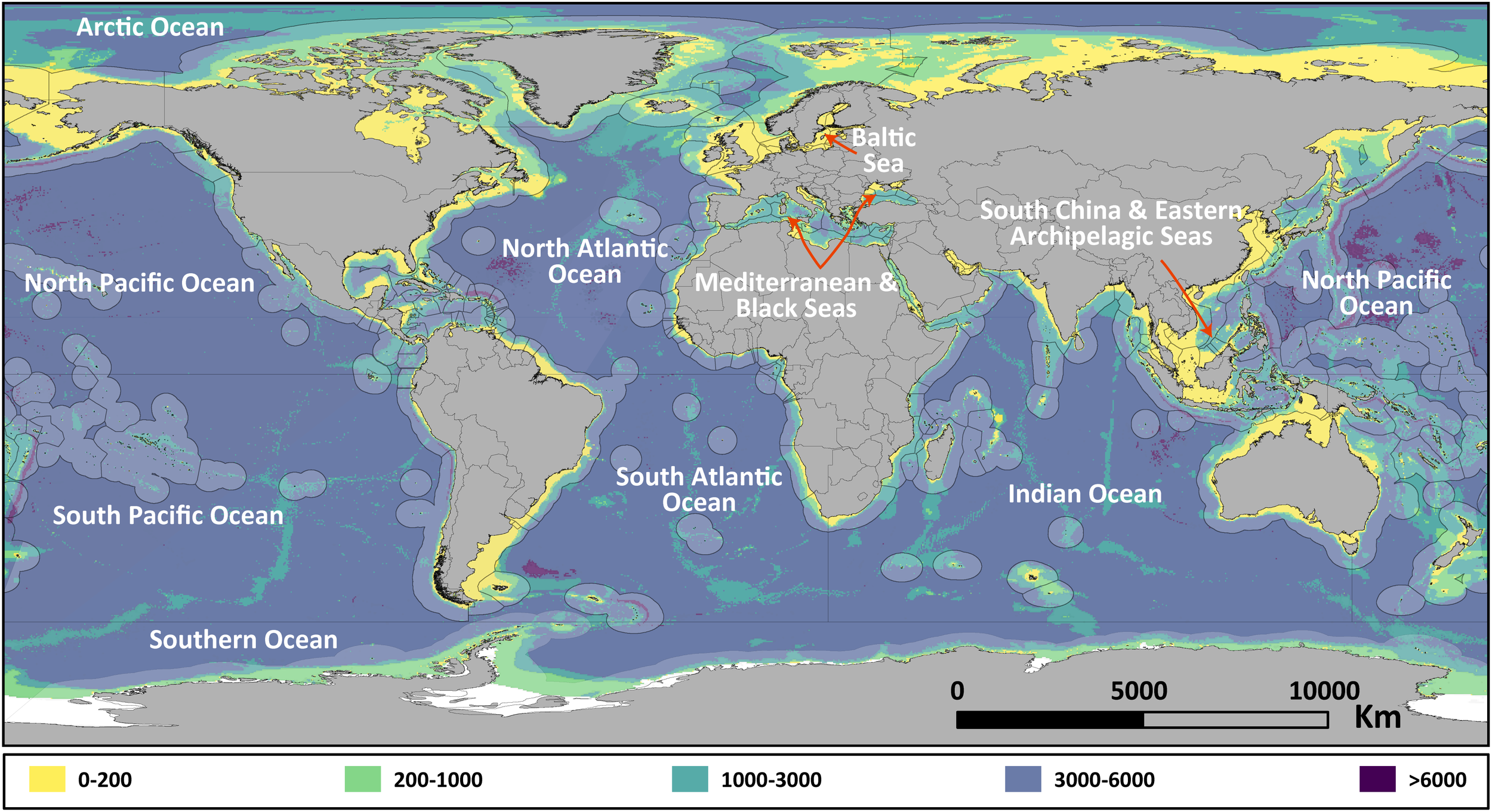
Distribution of different depth zones within the world ocean and seas and EEZ. The EEZ analysed this study includes all the area between a state’s coastline (delineated as zero depth based GEBCO_2024 bathymetry grid) and the outer limit of the corresponding EEZ. Territorial claims by sovereign states in the Southern Ocean are not considered EEZ. The depth zones are based on GEBCO_2024 bathymetry grid.
Five different depth zones were considered: the shallow zone (<200 m), the upper bathyal zone (200–1000 m), the lower bathyal zone (1000–3000 m), the abyssal zone (3000–6000 m) and the hadal zone (>6000 m), based on GEBCO_2024 bathymetric grid (Figure 1). Water depths <200 m correspond to nearshore locations and are often represented by the continental shelf. The upper bathyal zone is generally located on the upper slope and is characterised by sudden changes in slope gradient. The lower bathyal zone includes the mid-lower slope and continental rise, often representing a transition from continental margin to abyssal plain. The abyssal zone is represented largely by abyssal plains forming the majority of the global seafloor area. The hadal zone is primarily comprised of spatially isolated subduction trenches, fracture zones and deep basins.
A Python code was developed to accurately intersect GEBCO bathymetric and TID grid datasets with shapefiles representing the aforementioned global ocean and sea boundaries, EEZs, and defined depth zones. All data were reprojected to the Mollweide projection (ESRI:54009) to convert units from angular (decimal degrees) to linear units (meters) and to preserve accurate areas in both low and high latitudes. Based on the criteria of the Nippon Foundation-GEBCO Seabed 2030 Project, an area was considered ‘mapped’ if at least one sounding falls within a grid cell of 100x100 m at depths shallower than 1500 m, within a cell of 200x200 m at depths between 1500 m to 3000 m, within a cell of 400x400 m at depths between 3000 m to 5750 m, or within a cell of 800x800 m at depths greater than 5750 m (Mayer et al., 2018). In this study, the original resolution (15 arc-second, corresponding to 450 m resolution at the equator) of the GEBCO bathymetric and TID grids was used to maintain high accuracy of the analysis. A grid of 162 cells of 20 degrees each was generated to iteratively process cell-specific and allow memory-efficient computation. Each grid cell geometry was used to cut in-memory tiles of both the GEBCO bathymetric and TID grid rasters. These two tiles were then co-registered by reprojecting the bathymetric raster to match the resolution and spatial alignment of the TID using nearest neighbour resampling, ensuring that both datasets accurately overlay before stacking them together. A new band holding pixel-wise TID information was then added to the stack by iterating through each unique ocean and sea boundary polygon that intersected any given tile and assigning overlapping pixels a numeric code representing a specific ocean and sea while pixels outside were assigned a NaN (not a number) value. The same process was repeated with the EEZ, depth zones, and ABNJ, and corresponding bands were generated and added to the stack. This resulted in a multiband image holding information about the GEBCO TID mapping method (band 1), ocean and sea (band 2), EEZ (band 3), depth zones (band 4), and ABNJ (band 5) for each tile. Finally, a simple non-land pixels count (which has NaN in the ocean band) of all combinations of GEBCO TID, ocean and sea, EEZ, depth zones, and ABNJ in all the tiles provided coverage data which was then collated for all tiles in the grid before analysis. As the area was calculated based on the numbers and sizes of pixels, it gives the planar areal coverage of the mapped area but not the geodesic area. This may account for the differences between the values calculated in this study and the previously reported proportions of mapped areas worldwide. All coding has been developed using Python v3.12 (https://www.python.org) and open-source packages and is available at (https://github.com/yniyazi/global_seafloor_mapping). Maps were generated using ArcGIS Pro v3.2 (https://www.esri.com/en-us/home). Plots were made using Spyder v3.8 (https://www.spyder-ide.org).
Results and discussion
The Python scripts used for the calculation of the global seafloor mapping effort provide new insights into the current mapping status and progress and highlight priority areas for future mapping initiatives. Total mapping cover percentages presented here differ slightly from coverage values reported Seabed 2030 Project, T. N. F (2024), owing to methodological differences such as the resolution of the datasets used, definition of the mapped and unmapped areas, oceanic boundaries, and area calculation methods (planar vs geodesic) as described in the Data and Methods section. For example, total global mapping coverage in 2024 was 28.5% according to this study, whilst 26.1% was reported by Seabed 2030 (Seabed 2030 Project, T. N. F, 2024). Regardless, patterns are consistent with the general trends observed in global ocean mapping efforts and are valuable for guiding future mapping strategies.
Seafloor mapping efforts in the world’s ocean basins and seas
There has been a significant increase in the seafloor area mapped by direct measurement over the past six years, and MBES remained as the most used mapping method. In 2019, only 12.4% of the world’s seafloor was mapped, of which 12.2% was mapped by MBES (Figure 2, Supplementary Table S3). Since then, there has been a consistent increase each year in both direct measurement and area mapped with MBES. The growth is steady, and the areal coverage of 2024 is over twice that of 2019. Specifically, directly mapped area increased to 28.5% in 2024, of which 24.2% was mapped through MBES. The incremental increase for direct measurement ranges between 3-4% (average 3.2%) of global seafloor area each year, while the annual increment for MBES is smaller at about 2-3% (average 2.5%). This higher increase in the proportion of direct measurement area compared to the increase in MBES coverage is perhaps due to the wider application of Lidar and satellite-derived bathymetry in shallow zones, as well as the release of commercial seismic-derived bathymetric datasets in recent years (Lebrec et al., 2021; Harishidayat et al., 2024) (Figure 2b).
Figure 2
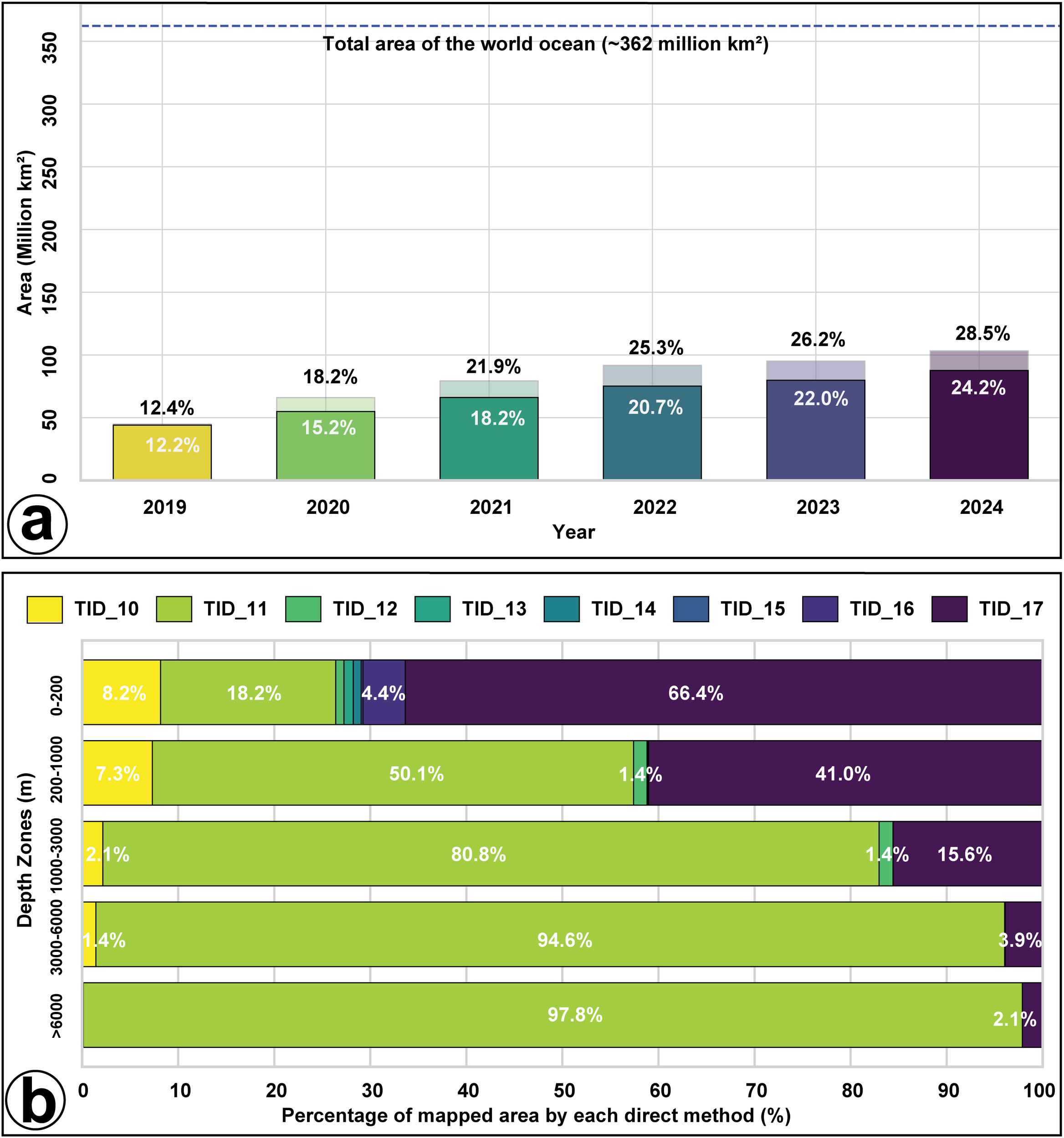
(a) Coverage and proportion of area mapped by all direct methods (semi-transparent bars) and MBES (bright bar) relative to the total world ocean and sea area, since 2019. (b) Proportion of area mapped by each direct method relative to total direct mapped area at different depth zones, in 2024. For the definition of TID and the corresponding codes, refer to Supplementary Table S1.
The proportion of seafloor area mapped by direct measurement differs across the ten ocean basins and seas (Figures 3 and 4, Supplementary Table S4). Among these regions, the SPO has the largest total areal coverage as it consists of 23.5% of the global ocean, followed by the NPO (21.4%) and the IO (19.6%). The NAO and SAO each comprise around 11% of the global ocean, while the AO and SO make up 4% and 6%, respectively. From a direct mapping perspective, the NAO and NPO demonstrate a clear and notable increase in mapping coverage over the past 6 years, especially in 2020 and 2021. By 2024, the proportional areal coverage of the NAO and NPO reaches 44.5% and 37.2%, respectively. This gradual year-on-year increase in mapping coverage is possibly due to the economic significance of these ocean basins and their proximity to high-income nations in Europe, North America, and Asia, resulting in increased investment in mapping to support maritime activities and research programs. By comparison, the SPO, SAO and IO show more gradual but steady mapping progress. By 2024, the proportional mapping coverage of the SAO reaches 28.1% of its total area, while the SPO and IO reach 23.4% and 17.5% respectively. Mapping coverage in the SPO and SAO is expected to increase due to research programs such as the iAtlantic Project (https://www.iatlantic.eu) and the All-Atlantic Ocean Research Alliance (Polejack et al., 2021), and the Schmidt Ocean Institute’s strategic framework for future exploration in this region (Schmidt Ocean Institute, 2024a). Although the vast size and challenging conditions in these remote regions make mapping efforts more logistically demanding, coverage in the IO has increased strongly since 2020, possibly related to increased international collaborations such as the Second International Indian Ocean Expedition (IIOE-2, https://iioe-2.incois.gov.in), data releases related to the search for MH370 (Picard et al., 2018; Hood and Beckley, 2019), and IO exploration projects (Werner et al., 2009; Jamieson et al., 2022; Niyazi et al., 2024; O’Hara, 2024). Furthermore, while the proportional cover percentage may appear relatively low, in absolute seabed area, more of the SPO has been mapped than the NAO. In the polar SO and AO, mapping progress has stabilised around the mid to upper 20% since 2022 (Supplementary Table S4) (Jakobsson et al., 2020; Dorschel et al., 2022). Achieving full coverage in these regions is challenging due to the presence of sea ice and extreme weather conditions during most of the year. The BS displays significant variation, particularly between 2022 and 2024, where its proportional coverage swings from 99.5%, to 28.9%, to 81.7%, implying a possible mis-categorisation of mapped data recorded in GEBCO TID during that period. The Med&BlaS shows a notably high mapping percentage starting in 2020, with mapping coverage reaching around 55%. However, since then, mapping progress appears to have plateaued. As much of the Med&BlaS lies within EEZs, this may reflect differences in mapping efforts or data contribution between countries bordering the Med&BlaS. Over the six-year period, the SCS&EAS region experienced an overall increase in mapping coverage from 4.81% in 2019 to 17.12% in 2024, almost quadrupling its mapped area. This significant growth reflects expanded data contribution and mapping initiatives, potentially due to the region’s ecological, economic, and geopolitical importance.
Figure 3
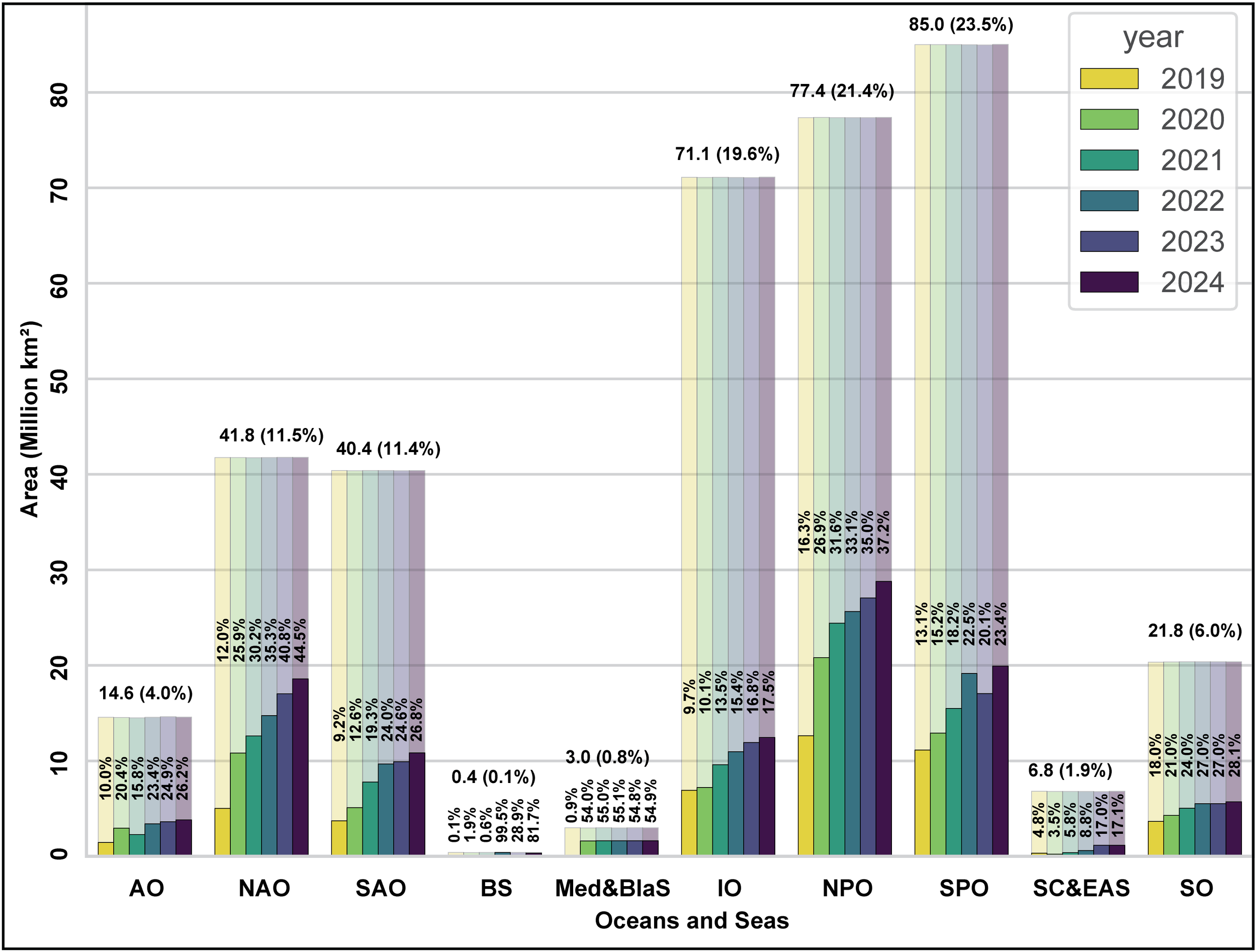
Accumulative coverage of mapped area in each ocean and sea, since 2019. Background (semi-transparent bars) is the absolute areal coverage of each ocean and sea, labelled horizontally with absolute area (km2) and percentage relative to the global ocean. Vertical labels above each bar represent the proportion of mapped area relative to the absolute areal coverage of each ocean and sea. AO, Arctic Ocean; BS, Baltic Sea; IO, Indian Ocean; Med&BlaS, Mediterranean Sea and Black Sea; NAO, North Atlantic Ocean; NPO, North Pacific Ocean; SAO, South Atlantic Ocean; SCS&EAS, South China Sea and Eastern Archipelagic Seas; SPO, South Pacific Ocean; SO, Southern Ocean.
Figure 4
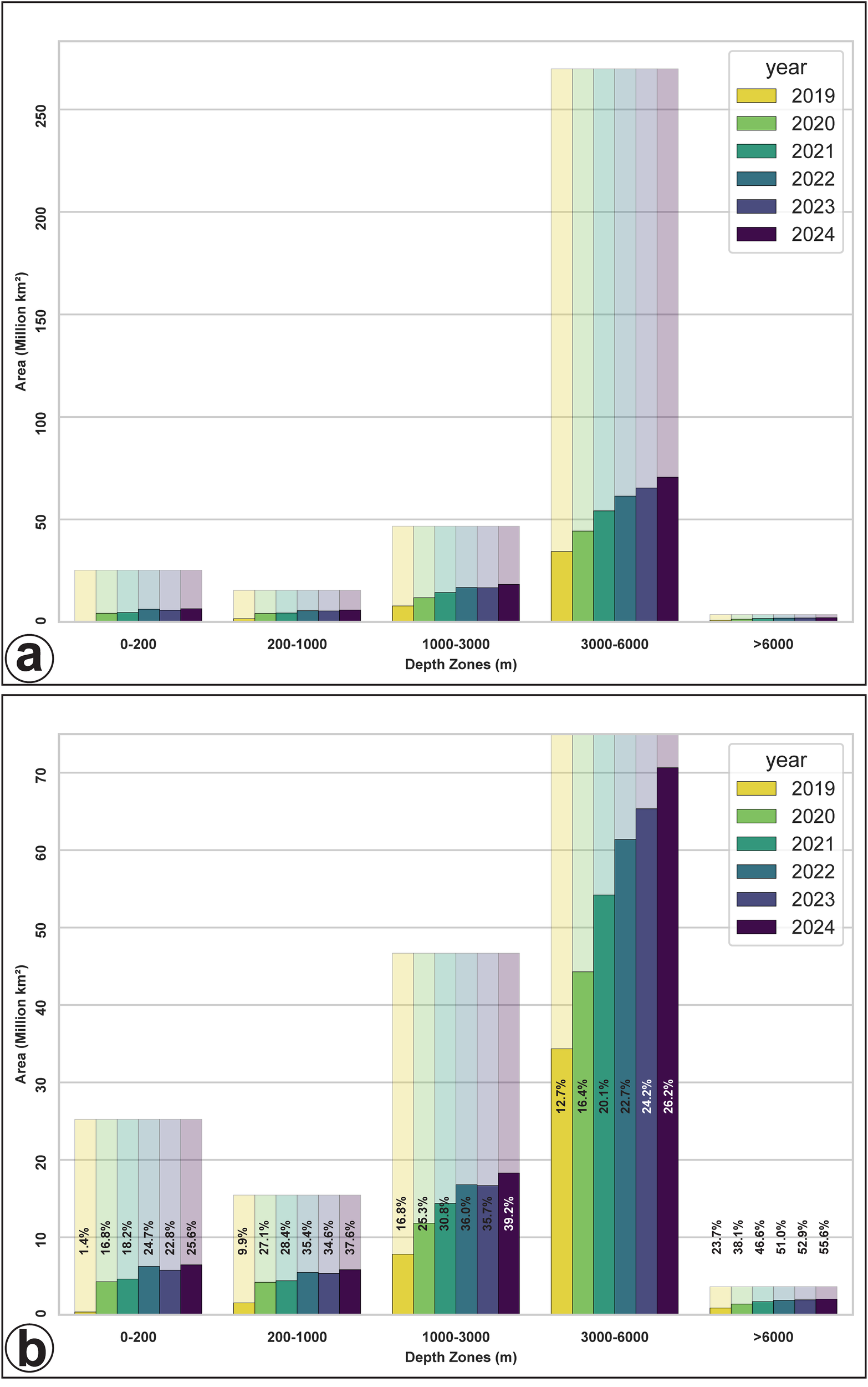
(a) Accumulative coverage of mapped area in different depth zones, since 2019. Background (semi-transparent bars) is the areal coverage of each depth zone, and the bright bars the areal coverage of mapped area. (b) Zoom in of (a). Vertical labels represent the proportion of directly mapped area relative to the areal coverage of each depth levels.
Proportion of direct mapping methods in each depth zone
Increases in mapping coverage vary with depth zone (Figures 4, 5, Supplementary Table S4). The shallow zone (<200 m) comprises ~7% of the global seafloor area, and the proportion of mapped area in this zone has consistently increased over the years, from 1.4% in 2019 to 25.7% by 2024, making up 6.3% of the global total mapped area. Notable progress occurred in 2020, with mapping coverage jumping to 16.7%. This increase likely reflects increased data collection and submission to GEBCO. Despite the relative accessibility and importance of this depth zone for marine navigation and coastal management, mapping coverage in this zone is lower than the average (28.1%) mapping coverage of global total seafloor. This could be explained by the narrower (< 2000 m, Mayer et al., 2018) swath width restricted by water depth. In addition, this lower percentage of publicly available data through GEBCO compared to deeper waters, may also relate to the fact that this depth zone almost always falls within the national jurisdiction of EEZs. Given the sensitivity of these areas to navigation regulations and national security and sovereignty, mapping efforts and data contribution largely depend on both resource availability to acquire data and national incentives to submit data. Furthermore, foreign research activity usually requires permit agreements for work within EEZs which may also influence mapping coverage in coastal areas.
Figure 5
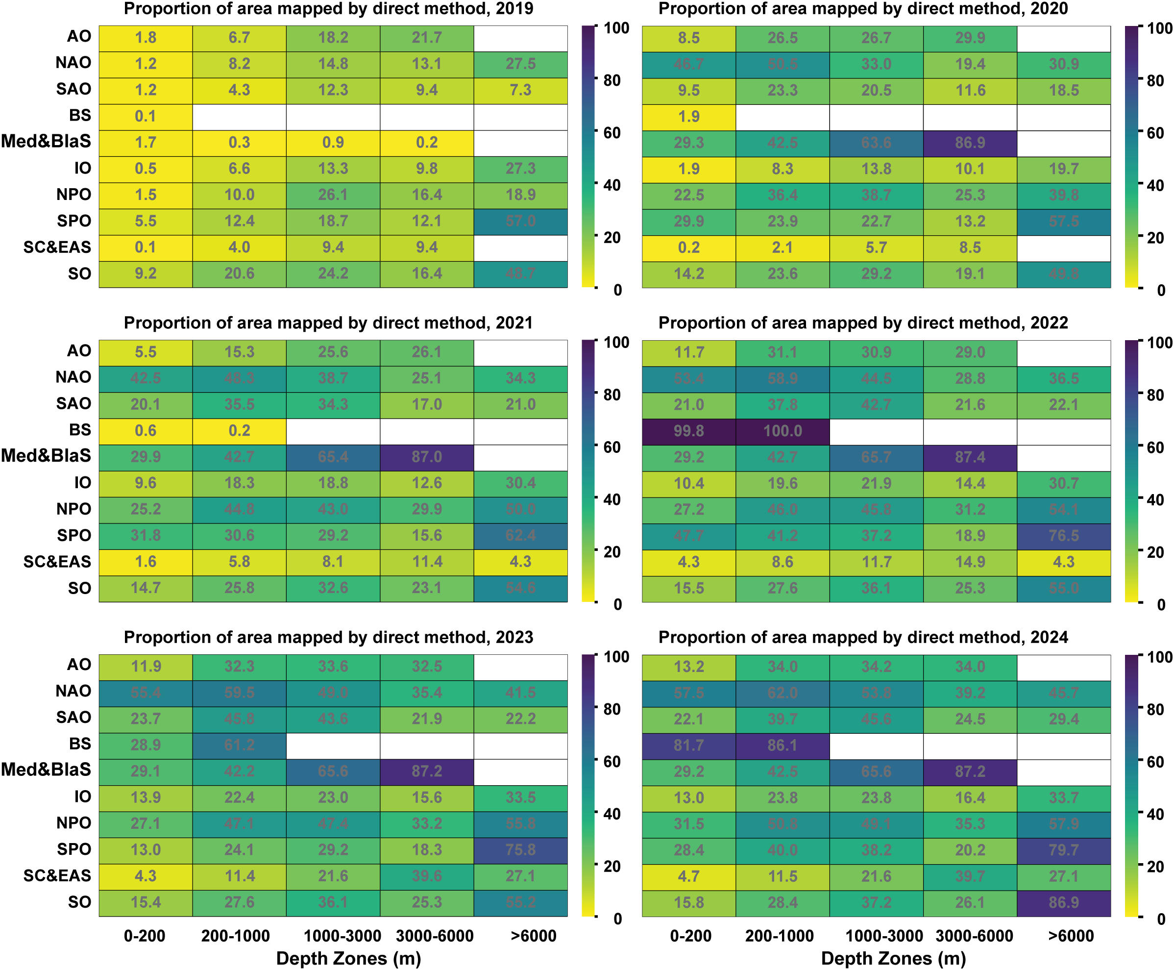
Heatmaps showing the proportion of mapped area within each ocean and sea, and in each depth zone from 2019 to 2024. Colour bar represents the proportion (%).
The upper and lower bathyal depth zones comprise 4.3% and 12.9% of the global total seafloor area, respectively. In the upper bathyal depth zone, mapping coverage increased from 9.9% in 2019 to 37.6% by 2024, rendering it one of the proportionally better-mapped depth zones along with the lower bathyal zone. Mapping efforts in the lower bathyal zone show similarly strong growth, increasing from 16.8% in 2019 to 39.2% by 2024. As such the upper and lower bathyal depth zones to comprise 5.6% and 17.7% of the global total mapping coverage, respectively. Significant resource exploration and extraction activities, including commercial fishing and deep-water hydrocarbon industries, occur at upper and lower bathyal depths, which could contribute to higher mapping coverage in these depth zones (Clark et al., 2016; Victorero et al., 2018). Intensification of mapping contributions from governments, research institutions, and the private sector since the launch of the Nippon Foundation-GEBCO Seabed 2030 Project may also play crucial role in the increase of mapping coverage in the bathyal zone (Jakobsson, 2020). The abyssal zone, comprising 74.5% of the global total seafloor area, has the largest areal proportion relative to the entire ocean area (Figure 4a). At abyssal depths, mapping coverage more than doubled from 12.7% in 2019 to 26.2% by 2024, comprising 68.4% of the global mapped area. In absolute terms, this equates to an area roughly the size of the Indian Ocean that has been mapped at abyssal depths (~71 million km2). As with bathyal depths, increasing industrial interest, primarily from deep-sea mining, and related research initiatives at abyssal depths may contribute to the growing mapping coverage in this depth zone (Volkmann et al., 2018; Simon-Lledó et al., 2020). Conversely, the hadal zone covers a very small (1.0%) area of the total global seafloor (Figure 4a), but has seen a rapid increase in direct mapping coverage, from 23.71% in 2019 to over 55.56% in 2024, attracting almost 2.0% of the global seafloor mapping effort and rendering it the depth zone with highest proportional mapping coverage. The dramatic increase reflects increased interest and specialized mapping and research initiatives for hadal features, aimed to the understanding of the extreme biological, ecological and geological conditions of the deepest trenches and troughs in the oceans (Jamieson et al., 2018; Stewart and Jamieson, 2018; Bongiovanni et al., 2022). Increase in mapping percentage in all the bathyal, abyssal and hadal zones, may also have been benefited from the development and integration of MBES technology with AUVs and uncrewed surface vessels (USVs) that have enhanced data collection efficiency and safety in remote and restricted areas (Kum et al., 2020).
The mapping methods employed also vary by depth zone, as shown by the GEBCO_2024 TID data (Figure 2b, Supplementary Table S1). The largest variety of methods used occurred in water depths <200 m. Of the direct mapping methods, a combination of various direct mapping methods is the most commonly utilised (TID_17, 66.4%), followed by MBES (TID_11, 18.2%) and SBMS (TID_10, 8.2%). In this depth zone, other methods such as satellite-derived bathymetry (TID_16), isolated sounding methods (TID_13) and seismic-derived bathymetry (TID_12) also contribute to mapping coverage (4.4%, 1.0% and 0.8%, respectively). This diversity of applied direct mapping methods is related to the availability of Lidar and optical methods to map clear, shallow waters, which light can easily penetrate. In the upper bathyal depth zone, the combined direct method (TID_17) remains significant, covering 41.0% of the mapped area. However, MBES becomes more dominant than in the shallowest zone, now representing 50.1% of the mapped area (Figure 2b). SBES covers 7.3%, while seismic-derived bathymetry (1.4%) and Electronic Navigation Chart (ENC) sounding (0.1%) represent minor contributions. The increase in MBES reflects a transition to acoustic mapping methods as the maximum water depth that light can readily penetrate is generally exceeded in waters beyond 200 m, prohibiting the use of optical mapping methods. In the lower bathyal zone, the proportion of seafloor mapping methods continues to shift, with MBES contributing 80.8% of the mapped area. The combined direct method decreases in proportion to 15.6%, while SBES (2.1%) and seismic-derived bathymetry (1.4%) also make increasingly smaller contributions. At abyssal depths, MBES dominates coverage, accounting for 94.6% of the mapped area. SBES and combined direct method contribute only minimal coverage, at 1.4% and 3.9%, respectively. The sharp decline in the variety of mapping methods highlights the advantages of MBES in meeting the technical requirements to map greater depths. In the hadal zone, MBES remains the primary mapping method, making up 97.8% of the mapped area. This extreme depth is almost entirely mapped through MBES, with very limited contributions from SBES (0.1%) and combined direct methods (2.1%). A heatmap comparison matrix of proportional area mapped by major ocean basin or sea versus depth zone is shown in Figure 5, providing spatial cross-referencing of the greatest increases in proportional mapping effort from 2019 to 2024.
Seafloor mapping efforts in the EEZs
The areal coverage of available bathymetric data for EEZs of the countries has increased from 5.7% in 2014, to 13.1% in 2019, and 33.2% in 2024 (Supplementary Table S5). The coverage of area mapped by direct method across EEZs varies significantly by sovereign state, location, water depth and economic status (Figures 6, 7). In general, states in the northern hemisphere have higher mapping coverage than those in the southern hemisphere (Figure 7).
Figure 6
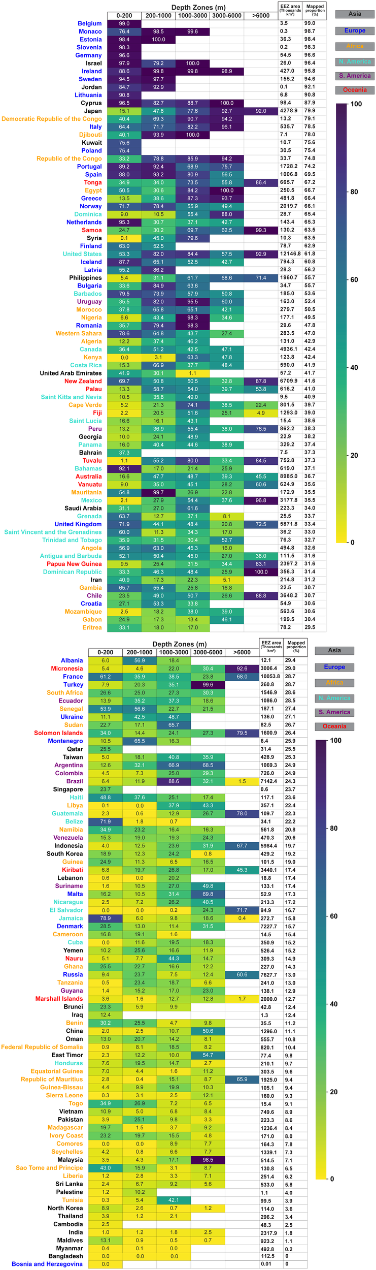
Proportion of mapped area in each Exclusive Economic Zone (EEZ) subdivided by different depth zones. The sovereign states are listed based on the proportion of total mapped area in their respective EEZ. The EEZ area includes all regions between a state’s coastline and the outer limit of its corresponding EEZ. Colours of the sovereign state names represent their continental locations.
Figure 7
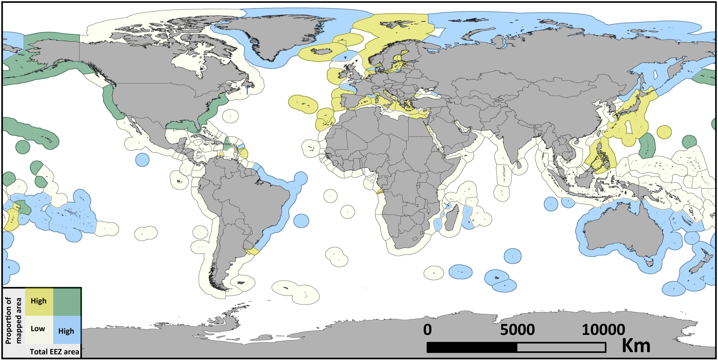
Bivariate map showing the proportion of total area mapped by direct method and total area of Exclusive Economic Zone (EEZ) for each nation. Both the total EEZ area and proportion of mapping is classified by equal interval method.
The majority of states with the highest proportion of seafloor area mapped by direct method are located in Europe. Coverage approaches 100% in shallow and upper bathyal waters for countries including Belgium, Monaco, and Estonia owing to their relatively small EEZs and strategic interest in coastal and marine economies. Despite the larger size and deeper depth, 95.8% of the Republic of Ireland EEZ is directly mapped owing to nationwide initiatives (O’Toole et al., 2022). At depths >1000 m, countries with larger marine territories (e.g. Norway, France, Portugal, Spain) still have high proportions of directly mapped areas, and mapping gaps are increasingly addressed with national initiatives led by their respective hydrographic offices and research institutes (Buhl-Mortensen et al., 2015; Míguez et al., 2019; Thierry et al., 2019; Moses and Vallius, 2020; Thorsnes et al., 2020; Dias, 2021) (Figure 6). Several European countries (e.g. United Kingdom, The Netherlands, France) have well-mapped shallow waters, but lag in mapping coverage of their deeper regions. These deeper regions likely correspond to their overseas territories located in distal oceanic areas compared to their relatively shallow adjacent continental shelves. For example, Denmark has relatively low mapping coverage as its territorial waters also include Greenland where mapping coverage is lower due to its remoteness, vast size and short weather window for marine operations. Bosnia and Herzegovina is unique, since it’s EEZ does not exceed water depths of 200 m, and has no publicly available bathymetry data.
Asia features a mix of high-income nations and low-middle-income countries with diverse EEZ sizes and geographic national priorities. Middle Eastern countries bordering the Red Sea and Persian Gulf, such as Israel, Jordan and Kuwait, show high mapping coverage, likely reflecting the importance of this area for shipping and commerce routes as well as resource assessment and extraction. In East Asia, Japanese territorial waters are particularly well mapped, with almost all (>92%) of its abyssal and hadal areas mapped, as well as over three-quarters of its lower bathyal zone surveyed by direct measurement. This reflects national mapping initiatives and international research in deeper waters; a key motivation being earthquake monitoring for risk assessment and hazard mitigation (Suyehiro et al., 2003). In contrast, its shallower zones are comparatively less well-mapped (<15%), reflecting a potential focus on economically valuable or strategically important areas. Indeed, many Asian EEZs are relatively poorly mapped, with less than 2% of India’s EEZ mapped to date. China also has a very low proportion of mapped area in its shallower waters, with only 2% and 2.5% mapped in shallow and upper bathyal depths respectively (Figure 6). However, China is likely to have mapped more of its EEZ than suggested by Figure 6 based on its resource availability, highlighting that not all seabed data is necessarily submitted for inclusion in the GEBCO grid. Instead, some data may be stored in secure national government repositories, especially data deemed to be nationally sensitive. Mapping coverage in Southeast Asian countries like Bangladesh, Myanmar, Cambodia, Thailand and Vietnam is limited, likely mirroring resource constraints.
African countries generally have low mapping coverage. Many EEZs remain largely unmapped likely owing to the high cost of marine mapping technologies and limited infrastructure (Bell et al., 2023). However, African countries known for offshore resources, and large-scale geomorphic features such as submarine canyons, fans, and landslides (e.g. Egypt, Morocco, the Democratic Republic of the Congo, Republic of the Congo, Nigeria, Algeria, Mauritania, Angola and Kenya), exhibit higher mapping coverage, likely driven by both industry-led and funded research initiatives (Babonneau et al., 2002; Schulz, 2003; Loncke and Mascle, 2004; Krastel et al., 2014; Ruffell et al., 2024). Djibouti and Egypt, which act as important shipping hubs and where seafloor mapping is a priority for navigation, also feature high mapping coverage.
In North America, the United States of America (USA) and Canada have strong mapping coverage in shallow and bathyal zones due to their advanced mapping technologies, strong track record of research funding, and strategic interests (Westington et al., 2019; Bell et al., 2023; Forbes, 2023). Deep-sea areas within their EEZs are partially mapped, some of which may relate to offshore resource activity (e.g. in the Gulf of Mexico). The USA, in particular, is well mapped across all depths, with over 50% of each depth zone mapped in its EEZ. In fact, it is the only country with a high total EEZ area that is also rated as a country with a high proportion of total area mapped by direct method (Figure 7). This could be attributed to national open-source initiatives such as the Rolling Deck to Repository (R2R, https://www.rvdata.us) and the Marine Geoscience Data System (MGDS, https://www.marine-geo.org) that ensure seafloor mapping data are regularly and efficiently submitted and are subsequently uploaded to GEBCO. Many South American countries (e.g. Peru, Colombia) have low mapping coverage, particularly in deeper depth zones. However, Uruguay has the highest mapped coverage proportionally for South America, likely due to the presence of the major port city of Montevideo and its relatively small EEZ which is located along an important shipping route (Krastel et al., 2011). Meanwhile, larger EEZs in South America, like those of Brazil and Argentina, have moderate mapping coverage focused on key economic areas (e.g., hydrocarbon exploration zones). In Chilean territorial waters, a high proportion of the hadal area has been mapped, possibly because of scientific interest in the Peru-Chile Trench (Fujii et al., 2013; Bongiovanni et al., 2022). Conversely, some Caribbean nations, such as the Bahamas, Barbados and Grenada, appear to have prioritized mapping shallow zones, potentially owing to the economic importance of fisheries and tourism in this region (Deville et al., 2003; Mulder et al., 2012)
In Oceania, high-income countries like Australia and New Zealand have relatively high overall coverage, benefiting from the activities of research institutions and international collaborations (Stuart Caie, 2023; Geoscience Australia, 2024). Some oceanic nations including The Kingdom of Tonga, the Independent State of Samoa and the Philippines (the latter is classed as Asia in this study) feature large mapping coverage, especially in deeper waters. This may be a function of specific research interest in features located in their EEZs (e.g. Tonga Trench and Philippine Trench) (Jamieson et al., 2024c). Globally, island nations stand out as a special case, especially those characterised by extensive maritime zones compared to their land mass and population, and their lower-income status (e.g. Seychelles, Maldives, Micronesia, Republic of Kiribati) (Jamieson et al., 2024a). Due to their vast size, these benefit from international collaborations to address data coverage gaps in EEZ (Jamieson et al., 2024a).
Seafloor mapping efforts in ABNJ
In ABNJ, mapping efforts similarly vary across ocean basins and depth zones (Figure 8). Nearly forty percent of the NAO’s ABNJ have been mapped, reinforcing that the NAO is the best mapped of the world’s ocean basins by proportion (Figure 8a). The AO is the least mapped of the different ocean basins’ ABNJ at 9.2%, likely owing to distance from land and extensive sea-ice coverage for the central Arctic during most of the year, which restricts research opportunities (Ramirez-Llodra et al., 2024). Similarly, only 16% of the IO’s ABNJ have been mapped, an expected result given the recognised need for more research in this region, particularly in the southern IO, which holds a large proportion of ABNJ (Thomas et al., 2024). Proportional ABNJ mapping coverage in the SAO, NPO, SPO, and SO ranges between 23.1% and 27.9%.
Figure 8
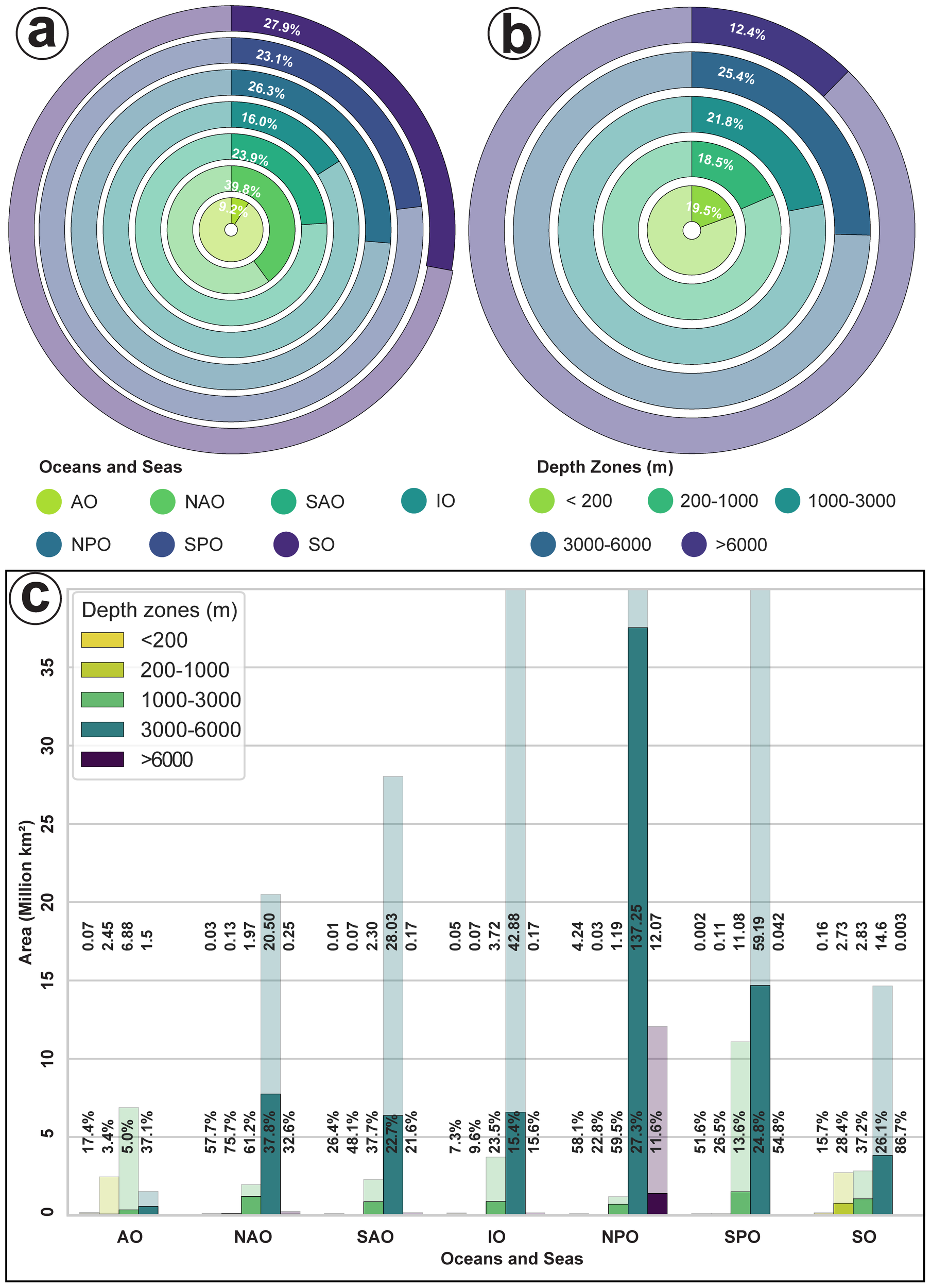
Proportion of mapped area of Area Beyond National Jurisdiction (ABNJ) within each ocean (A) and each depth zone (B). (C) Total and mapped ABNJ area in each ocean at different depth zones. Upper labels represent the total area (million km2) of ABNJ in each ocean at different depths, lower labels represent the proportion (%) of area mapped. The area bar plots are cut at 40 million km2 to better highlight the oceans and depths with lower values.
Evaluating ABNJ mapping coverage by depth zone, the abyssal zone is best proportionally mapped – 25.4% across all ocean basins (Figure 8b) and up to 37.8% in the NAO (Figure 8c) – despite also representing the largest depth zone by total area in ABNJ. The lower bathyal zone is also relatively well mapped (21.8%), given that it accounts for a large portion of ABNJ. Shallow and hadal depths account for very small portions of ABNJ, since the global continental shelf and many hadal trenches largely lie within EEZs. Yet only 19.5% and 12.4% of these depths have been mapped in ABNJ, respectively (Figure 8b).
Considering ABNJ mapping efforts by both depth and ocean basin reveals significant variability in coverage (Figure 8c). Apart from in the IO and polar regions, the shallow zone is relatively well mapped in most ocean basins (up to 51.6% in the SPO’s ABNJ), however, this is likely a feature of the very small absolute areas for depths <200 m in ABNJ (generally <0.1 million km2). Only the NPO’s ABNJ has a greater absolute area for depths <200 m, 4.24 million km2, likely owing to the tectonic evolution and high number of shallow seamounts in the region (Wessel et al., 2010; Kim and Wessel, 2011; Yesson et al., 2011). The upper bathyal zone is the best mapped for ABNJ in the NAO (more than 75%) and SAO (48.1%), while only around one-quarter of the NPO, SPO and SO’s upper bathyal depth ABNJ is mapped. Lower bathyal depths are proportionally well mapped in NAO and NPO ABNJ (>59%), and SAO and SO ABNJ (>37%). Conversely, while the lower bathyal zone is the largest depth zone in terms of absolute area for the AO’s ABNJ, only 5% of this area has been mapped. In absolute area, mapping coverage of abyssal regions in ABNJ is high in the NPO and SPO. Proportionally, around a quarter or more of abyssal area has been mapped in most ocean basins apart from the IO (15.4%), where ABNJ mapping coverage is low generally. Despite their small absolute area, hadal zones feature high mapping coverage. For example, the hadal zone has the highest proportion of mapped area in the SPO’s ABNJ (54.8%). Similarly, the NPO is known for its extensive hadal areas, comprising over 12 million km2 of the NPO’s ABNJ, including trenches, deep basins and fracture zones (Jamieson and Stewart, 2021) and as such is a key target for deep-sea research initiatives. However, only 11.6% of its hadal ABNJ has been mapped to date, reflecting the magnitude of this depth zone in the NPO. The higher mapping proportions at lower bathyal, abyssal and hadal depths in these ABNJ may reflect mapping and research initiatives that targeted prominent seafloor features such as mid-ocean ridges, fracture zones, seamounts, hydrothermal vents and submarine canyons (Somoza et al., 2021; Bond et al., 2023; Swanborn et al., 2023; Jamieson et al., 2024a, 2024b).
Why direct mapping matters
Differences between unmapped (where existing bathymetry has only been predicted by interpolation and indirect depth measurements) and mapped (where bathymetry is derived from direct mapping methods) areas were assessed using a depth difference map generated by subtracting the unmapped area (covered by the SRTM15+ model) of the GEBCO_2022 bathymetry grid from the mapped (measured) area in the GEBCO_2024 bathymetry grid. The GEBCO_2022 TID grid was selected to evaluate the depth discrepancy to avoid TID mis-categorisation present in the previous TID grids.
Overall, the vast majority (85.7%) of the predicted depths deviate from the measured depths by no more than ±100 m, suggesting the SRTM15+ model is consistent with its estimated level of accuracy in these areas (Figure 9a). The depth differences are within 100 to 500 m in 14% of the compared area, and considering the full depth of the ocean, this difference could be deemed minor, especially in the abyssal and hadal zones. Depth differences in the remaining 0.3% mostly range between 500 to 2000 m. Within the 0–500 m offset range, the measured depth value was deeper than the predicted value in 62.1% of the cases, and shallower than the predicted value in 37.6% of the cases (Figure 9a).
Figure 9
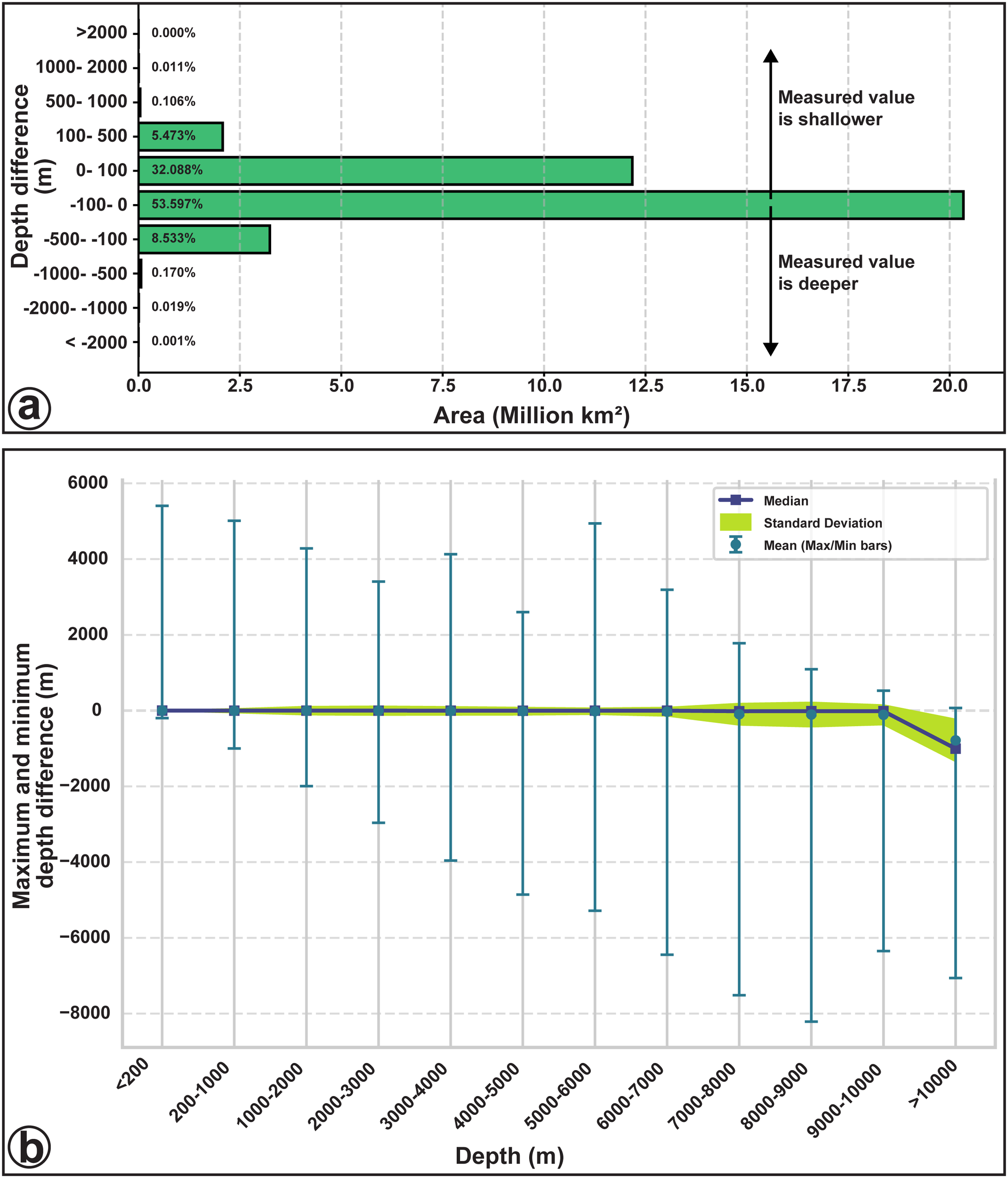
Differences in depth value from the mapped and unmapped grids, calculated by subtracting GEBCO_2022 grid from the GEBCO_2024 grid for the specific area that is considered unmapped in in the former and mapped in the latter compilation. (a) Distribution histogram showing the depth differences and corresponding area. (b) Distribution histogram showing the depth maximum, minimum and average differences within specific depth intervals.
However, discrepancies between the depth value of the unmapped and directly mapped areas are depth-dependent (Figure 9b). The absolute average differences between mapped and predicted grids increase from less than 3 m in the shallow and upper bathyal zone (200–1000 m), to an extreme of 4161 m in depths greater than 10,000 m (Figure 9b). Although the predicted and mapped depth values are comparable for shallower depths, average absolute depth differences start to increase at hadal depths, indicating increased discrepancy between indirectly and directly mapped depth values in deeper waters. Across all depths, outliers can be found in either direction though trending towards deeper measured values with depth.
Outlook and recommendations
The results of this study highlight the importance of employing direct mapping methods to both verify and, where necessary, correct the recorded seafloor bathymetry. Acquiring these accurate depth data is critical for ensuring safety in maritime navigation and industries, identifying natural resource targets for exploitation, understanding the structure and drivers of seafloor environments, conservation, and addressing important marine ecological questions (e.g. species distributions, connectivity, habitat delineation) (Wölfl et al., 2019). Such applications of seafloor mapping range from local to global importance and contribute to the UN’s Sustainable Development Goal 14 (Life Below Water) to “conserve and sustainably use the oceans, seas and marine resources”. The past five years have seen a strong increase in the availability of directly mapped seafloor data globally, strengthened by global initiatives and international collaborations in data acquisition, processing and sharing. This study showed a trajectory of growth in bathymetric data coverage across different ocean basins and seas, EEZs, ABNJ and depth zones. While this steady growth is promising, we highlight the importance of sustaining and striving to improve upon the established trajectory. Since the start of the UN Ocean Decade, there has been a renewed incentive to map the seafloor, spearheaded by the Seabed 2030 project (Mayer et al., 2018; Jakobsson, 2020). However, with the total area mapped currently sitting at 28.5% as per this study (24.2% MBES) of the global ocean, a significant effort is still required to achieve the ambitious goal set out by this initiative of mapping the entire world ocean by 2030 (Mayer et al., 2018).
At the average rate of direct mapping progress since 2019 of ∼3.2% per year (Figure 2a), it would take over 22 years for GEBCO’s full seafloor map to be complete with current resolution, if the new added coverage is not concurrent with previously mapped areas. As with other recent reviews of marine research progress (Bridges et al., 2023; Ramirez-Llodra et al., 2024; Thomas et al., 2024), we have found extensive spatial inconsistencies in the availability and quality (direct vs indirect) of data across different ocean basins, EEZs and depth zones. To address this, it is imperative moving forward that we target and explore new areas, rather than revisiting regions that have already been mapped to a very high quality, such as the Mariana Trench (Greenaway et al., 2021; Bongiovanni et al., 2022) and the Drake Passage (Dorschel et al., 2022). Initiatives to map new areas have already yielded impressive results and interesting discoveries in seafloor geomorphology: from trans-oceanic expeditions that have mapped extensive transects (e.g. Trans-Pacific Transit Expedition which mapped 373,732 km2 of seafloor, an area similar in size to Japan (Jamieson et al., 2024a)), to the mapping of newly discovered seafloor features (e.g. ‘Eye of Sauron’ caldera (O’Hara, 2024)). The sheer size of these new features are not insignificant, with one newly discovered seamount recently mapped from the Nazca Ridge covering ∼70 km2 in area and reaching over 3100 m in height (Schmidt Ocean Institute, 2024b), and their discovery supports the identification of high priority areas for protection. Research vessels could also utilise their transit time to map new areas by using the BathyGlobe GapFiller or similar algorithms that provide automatic adjustment of transit lines reduce duplication of existing data but rather slightly overlap prior mapping coverage (Galceran and Carreras, 2012; Ware et al., 2023).
Beyond mapping for scientific research, the support and mobilisation of the global fleet of vessels is also crucial to support this initiative (Coley, 2022). In this way, mapping new areas may be achieved by capitalising on existing technology and predetermined vessel transits, whereby shipping fleets and other operators with MBES or other direct mapping equipment are encouraged to continue mapping as they are transiting from one area to another. A wide variety of organisations traverse the ocean, representing science, industries, governments, philanthropy, non-governmental organisations, and more. Harnessing the resources and enterprise of each of these groups is essential to utilise the global fleet of equipped vessels to its full potential, including merchant ships, military ships, cruise liners, fishing vessels, ferries, private yachts, and sailing boats (Wölfl et al., 2019). This, along with the application of the BathyGlobe GapFiller or similar programs, will increase the coverage in the non-target regions during the transit. Furthermore, various studies have demonstrated the use of vessels of opportunity, that is ships that are not primarily scientific vessels but can carry devices to measure environmental and acoustic variables, in supplementing scientific research in this way (Wright and Baldauf, 2016; Haris et al., 2021).
Uneven mapping coverage within the EEZs of sovereign states and ABNJ in different depth zones indicate priorities should be given to specific regions and depths to catch up with the average global mapping coverage. As some of the Asian, African and South American states have the least coverage in almost all depth zones, a strategic initiative to deploy research vessels to this region will help with the mapping efforts. Schmidt Ocean Institute (2024a)‘s research plans set up until 2033 highlight such necessity and will help to increase mapping coverages in both EEZs and ABNJ in the southern hemisphere. Simplifying the associated logistical paperwork and regulatory processes in EEZs would significantly reduce barriers, encouraging collaboration and efficient execution of mapping projects. In addition, technological innovations to produce low-cost marine robotics, such as low-logistics AUVs will help low-income countries to map their EEZs (Wölfl et al., 2019; Osuka et al., 2021).
Finally, while the importance of a complete global ocean map has been emphasised (Coley, 2022), there is a need to also look beyond the UN Ocean Decade and the Seabed 2030 targets, to understand the potential applications of such a resource and begin laying plans to build upon this achievement. Our mission to understand our ocean is not complete once the entire seafloor has been mapped, rather it will provide us with a new tool to realise new research ambitions. Potential applications may include the overlaying of biological models to better study the local-to-global connectivity of our ocean and support marine spatial planning, especially in the face of a changing climate (Worm et al., 2006; Harris and Baker, 2019; Frazão Santos et al., 2020). Highlighting these ambitions now may help to further incentivise increased data acquisition, processing and sharing for a global map of the seafloor.
Conclusion
In conclusion, mapping coverage varies substantially across depth zones of ocean basins, EEZs, and ABNJ. The NAO and NPO have the highest proportional mapping coverage of up to 44.5% and 37.2%, respectively, while the AO, SAO, SPO and SO have mapping coverage of nearly 30%. The IO is the least mapped ocean with only 17.5% mapped. The hadal zone is mapped to a high proportion of 55.6%, while the upper and lower bathyal depths are up to 39%. Meanwhile, only around one-quarter of the shallow and abyssal zones are mapped. The types of direct mapping methods used also vary by depth, with MBES identified as an increasingly important tool for mapping in deeper ocean depths. Mapping coverage variation in EEZs is likely influenced by economic resources, technological capacity, and geographic priorities. Europe and North America lead in mapping efforts, while Africa, Asia, and Oceania face challenges in achieving comprehensive mapping, particularly in deep-sea zones. Meanwhile, low proportions of mapped ABNJ tend to correspond with more remote and inaccessible ocean basins and depth zones that are rarely prioritised for marine research and have low maritime activity (e.g. southern IO and central AO). Applying the average mapping progress of 3.2%, mapping of the whole seafloor will be completed by 2047, which is well beyond the targets of the SEABED 2030 and UN Decade of Ocean Science for Sustainable Development. More effort and resources must be prioritised for those areas with low mapping coverage to accomplish full bathymetric seafloor coverage in a reasonable timeframe.
Statements
Data availability statement
The original contributions presented in the study are included in the article/Supplementary Material, further inquiries can be directed to the corresponding author/s.
Author contributions
YN: Conceptualization, Data curation, Formal analysis, Investigation, Methodology, Software, Visualization, Writing – original draft, Writing – review & editing. ET: Formal analysis, Validation, Writing – original draft, Writing – review & editing. NP: Data curation, Software, Validation, Writing – review & editing. DS: Formal Analysis, Validation, Writing – original draft, Writing – review & editing. HS: Funding acquisition, Project administration, Supervision, Validation, Writing – review & editing. AJ: Conceptualization, Funding acquisition, Project administration, Supervision, Validation, Writing – review & editing.
Funding
The author(s) declare that financial support was received for the research and/or publication of this article. Data analysis and writing of this study were supported by the Minderoo-UWA Deep-Sea Research Centre, funded by the Minderoo Foundation and Inkfish LLC. The funder was not involved in the study design, collection, analysis, interpretation of data, the writing of this article, or the decision to submit it for publication.
Acknowledgments
We thank Pauline Weatherall from the British Oceanographic Data Centre and Jaya Roperez from Inkfish for assistance with the datasets.
Conflict of interest
Author HS was employed by Kelpie Geoscience Ltd.
The remaining authors declare that the research was conducted in the absence of any commercial or financial relationships that could be construed as a potential conflict of interest.
Generative AI statement
The author(s) declare that no Generative AI was used in the creation of this manuscript.
Publisher’s note
All claims expressed in this article are solely those of the authors and do not necessarily represent those of their affiliated organizations, or those of the publisher, the editors and the reviewers. Any product that may be evaluated in this article, or claim that may be made by its manufacturer, is not guaranteed or endorsed by the publisher.
Supplementary material
The Supplementary Material for this article can be found online at: https://www.frontiersin.org/articles/10.3389/fmars.2025.1543885/full#supplementary-material
References
1
Anderson J. Peters K. (2016). Water worlds: Human geographies of the ocean. London, England: Ashgate Publishing. doi: 10.4324/9781315547619
2
Babonneau N. Savoye B. Cremer M. Klein B. (2002). Morphology and architecture of the present canyon and channel system of the Zaire deep-sea fan. Mar Pet Geol19, 445–467. doi: 10.1016/S0264-8172(02)00009-0
3
Beaman R. J. O’Brien P. E. Post A. L. De Santis L. (2010). A new high-resolution bathymetry model for the Terre Adélie and George V continental margin, East Antarctica. Antarct Sci.23, 95–103. doi: 10.1017/s095410201000074x
4
Bell K. L. C. Quinzin M. C. Amon D. Poulton S. Hope A. Sarti O. et al . (2023). Exposing inequities in deep-sea exploration and research: results of the 2022 Global Deep-Sea Capacity Assessment. Front. Mar Sci.10. doi: 10.3389/fmars.2023.1217227
5
Bond T. Niyazi Y. Kolbusz J. L. Jamieson A. J. (2023). Habitat and benthic fauna of the Wallaby-Cuvier escarpment, SE Indian ocean. Deep Sea Res. Part II210, 105299. doi: 10.1016/J.DSR2.2023.105299
6
Bongiovanni C. Stewart H. A. Jamieson A. J. (2022). High-resolution multibeam sonar bathymetry of the deepest place in each ocean. Geosci Data J.9, 108–123. doi: 10.1002/GDJ3.122
7
Bridges A. E. H. Howell K. L. Amaro T. Atkinson L. Barnes D. K. A. Bax N. et al . (2023). “Review of the central and south atlantic shelf and deep-sea benthos: science, policy, and management,” in Oceanography and Marine Biology: An Annual Review, vol. 61. (Boca Raton: CRC Press), 127–218. doi: 10.1201/9781003363873-5
8
Buhl-Mortensen L. Buhl-Mortensen P. Dolan M. F. J. Holte B. (2015). The MAREANO programme – A full coverage mapping of the Norwegian off-shore benthic environment and fauna. Marine Biol. Res.11, 4–17. doi: 10.1080/17451000.2014.952312
9
Clark M. R. Althaus F. Schlacher T. A. Williams A. Bowden D. A. Rowden A. A. (2016). The impacts of deep-sea fisheries on benthic communities: a review. ICES J. Marine Sci.73, i51–i69. doi: 10.1093/ICESJMS/FSV123
10
Coley K. (2022). A global ocean map is not an ambition, but a necessity to support the ocean decade. Mar Technol. Soc. J.56, 9–12. doi: 10.4031/MTSJ.56.3.3
11
Costello M. J. Cheung A. De Hauwere N. (2010). Surface area and the seabed area, volume, depth, slope, and topographic variation for the world’s seas, oceans, and countries. Environ. Sci. Technol.44, 8821–8828. doi: 10.1021/es1012752
12
Deville E. Battani A. Griboulard R. Guerlais S. Herbin J. P. Houzay J. P. et al . (2003). The origin and processes of mud volcanism: New insights from Trinidad. Geol Soc. Spec Publ216, 475–490. doi: 10.1144/GSL.SP.2003.216.01.31
13
Dias T. G. (2021). “Program SEAMAP 2030: 100% of the portuguese maritime spaces mapped by 2030,” in The International Hydrographic Review, 159–168. Available at: https://journals.lib.unb.ca/index.php/ihr/article/view/33112 (Accessed December 4, 2024).
14
Dierssen H. M. Theberge A. E. (2016). “Bathymetry: seafloor mapping history,” in Encyclopedia of Natural Resources: Water, (Taylor & Francis), 644–648. doi: 10.1081/e-enrw-120047531
15
Dodds K. Hemmings A. D. (2015). “Polar Oceans: Sovereignty and the contestation of territorial and resource rights,” in Routledge Handbook of Ocean Resources and Management, Routledge, London, 576–591. doi: 10.4324/9780203115398-38
16
Dorschel B. Hehemann L. Viquerat S. Warnke F. Dreutter S. Tenberge Y. S. et al . (2022). The international bathymetric chart of the southern ocean version 2. Sci. Data9, 275. doi: 10.1038/s41597-022-01366-7
17
Flanders Marine Institute (2021). Global Oceans and Seas, version 1. Available online at: https://www.marineregions.org/ (Accessed December 4, 2024).
18
Flanders Marine Institute (2023). Maritime Boundaries Geodatabase: Maritime Boundaries and Exclusive Economic Zones (200NM), version 12. Available online at: https://www.marineregions.org (Accessed December 4, 2024).
19
Flanders Marine Institute (2024). Maritime Boundaries Geodatabase: High Seas, version 2. Available online at: https://www.marineregions.org/ (Accessed December 4, 2024).
20
Forbes A. R. (2023). Canadian Bathymetric Gap Analysis and the Comparison of Barometric Pressure Enhanced Predicted Tides to Ellipsoid Referenced Hydrographic Surveys. Available online at: https://tspace.library.utoronto.ca/handle/1807/130315 (Accessed December 4, 2024).
21
Frazão Santos C. Agardy T. Andrade F. Calado H. Crowder L. B. Ehler C. N. et al . (2020). Integrating climate change in ocean planning. Nat. Sustainability3, 505–516. doi: 10.1038/s41893-020-0513-x
22
Fujii T. Kilgallen N. Rowden A. Jamieson A. (2013). Deep-sea amphipod community structure across abyssal to hadal depths in the Peru-Chile and Kermadec trenches. Mar Ecol. Prog. Ser.492, 125–138. doi: 10.3354/meps10489
23
Galceran E. Carreras M. (2012). “Efficient seabed coverage path planning for ASVs and AUVs,” in IEEE International Conference on Intelligent Robots and Systems. Vilamoura-Algarve, Portugal, 88–93. doi: 10.1109/IROS.2012.6385553
24
Geoscience Australia (2024). Australia’s Seabed: How much is mapped? A national metadata assessment – 2024.
25
Greenaway S. F. Sullivan K. D. Umfress S. H. Beittel A. B. Wagner K. D. (2021). Revised depth of the Challenger Deep from submersible transects; including a general method for precise, pressure-derived depths in the ocean. Deep Sea Res. Part I178, 103644. doi: 10.1016/J.DSR.2021.103644
26
Halpern B. S. Frazier M. Afflerbach J. Lowndes J. S. Micheli F. O’Hara C. et al . (2019). Recent pace of change in human impact on the world’s ocean. Sci. Rep.9, 11609. doi: 10.1038/s41598-019-47201-9
27
Haris K. Kloser R. J. Ryan T. E. Downie R. A. Keith G. Nau A. W. (2021). Sounding out life in the deep using acoustic data from ships of opportunity. Sci. Data8, 1–23. doi: 10.1038/s41597-020-00785-8
28
Harris P. T. Baker E. (2019). Seafloor Geomorphology as Benthic Habitat: GeoHab Atlas of Seafloor Geomorphic Features and Benthic Habitats. Philadelphia, PA: Elsevier Science Publishing, 1–1030. doi: 10.1016/C2017-0-02139-0
29
Harishidayat D. Niyazi Y. Stewart H. A. Al-Shuhail A. Jamieson A. J. (2024). Submarine canyon development controlled by slope failure and oceanographic process interactions. Sci. Rep.. 14, 18486. doi: 10.1038/s41598-024-69536-8
30
Heezen B. C. Tharp M. (1957). Physiographic diagram, Atlantic Ocean. Available online at: https://nla.gov.au/nla.obj-3005098339/view (Accessed December 11, 2024).
31
Heezen B. C. Tharp M. Ewing M. (1959). The Floors of the Oceans: I. The North Atlantic. Geological Society of America. doi: 10.1130/SPE65
32
Hood R. R. Beckley L. E. (2019). The second international Indian ocean expedition (IIOE-2): motivating new exploration in a poorly understood ocean basin (Volume 1). Deep Sea Res. Part II161, 2–4. doi: 10.1016/J.DSR2.2019.04.009
33
Jakobsson M. Mayer L. A. Bringensparr C. Castro C. F. Mohammad R. Johnson P. et al . (2020). The international bathymetric chart of the arctic ocean version 4.0. Sci. Data7, 176. doi: 10.1038/s41597-020-0520-9
34
Jamieson A. (2015). The Hadal Zone: Life in the deepest oceans. Cambridge, England: Cambridge University Press. doi: 10.1017/CBO9781139061384
35
Jamieson A. J. Fang J. Cui W. (2018). Exploring the hadal zone: recent advances in hadal science and technology. Deep Sea Res. Part II: Topical Stud. Oceanography155, 1–3. doi: 10.1016/J.DSR2.2018.11.007
36
Jamieson A. J. Steward H. A. Kolbusz J. L. Nester G. Swanborn D. Javier M. (2024a). Nova Canton Trough Expedition Report (Inkfish Open Ocean Program), Zenodo. Available at: https://zenodo.org/records/14099757.
37
Jamieson A. J. Stewart H. A. (2021). Hadal zones of the Northwest Pacific Ocean. Prog. Oceanogr190, 102477. doi: 10.1016/j.pocean.2020.102477
38
Jamieson A. J. Stewart H. A. Bond T. Kolbusz J. L. Nester G. (2024b). Trans-Pacific Transit Expedition Report (Inkfish Open Ocean Program), Zenodo. doi: 10.5281/ZENODO.14103855
39
Jamieson A. J. Stewart H. A. Kolbusz J. L. Swanborn D. Nester G. (2024c). Tonga Trench Expedition Report (Inkfish Open Ocean Program), Zenodo. doi: 10.5281/zenodo.14094650
40
Jamieson A. J. Stewart H. A. Weston J. N. J. Lahey P. Vescovo V. L. (2022). Hadal biodiversity, habitats and potential chemosynthesis in the Java Trench, Eastern Indian ocean. Front. Mar Sci.9. doi: 10.3389/FMARS.2022.856992
41
Jupp D. L. B. (1988). “Background and extensions to depth of penetration (DOP) mapping in shallow coastal waters,” in The Symposium on Remote Sensing of the Coastal Zone. Queensland, Australia.
42
Kim S. S. Wessel P. (2011). New global seamount census from altimetry-derived gravity data. Geophys J. Int.186, 615–631. doi: 10.1111/j.1365-246X.2011.05076.x
43
Klein E. Hadré E. Krastel S. Urlaub M. (2023). An evaluation of the General Bathymetric Chart of the Ocean in shoreline-crossing geomorphometric investigations of volcanic islands. Front. Mar Sci.10. doi: 10.3389/fmars.2023.1259262
44
Krastel S. Böttner C. Cartigny M. Feldens P. Fu L. Glogowski S. et al . (2014). Morphology, processes and geohazards of giant landslides in and around Agadir Canyon, northwest Africa - Cruise MSM32 - September 25 - October 30, 2013 - Bremen (Germany) - Cádiz (Spain). doi: 10.2312/CR_MSM32
45
Krastel S. Wefer G. Hanebuth T. J. J. Antobreh A. A. Freudenthal T. Preu B. et al . (2011). Sediment dynamics and geohazards off Uruguay and the de la Plata River region (northern Argentina and Uruguay). Geo-Marine Lett.31, 271–283. doi: 10.1007/S00367-011-0232-4
46
Krogh A. (1934). Conditions of life in the ocean. Ecol. Monogr4, 421–429. doi: 10.2307/1961648
47
Kum B. C. Shin D. H. Jang S. Lee S. Y. Lee J. H. Moh T. J. et al . (2020). Application of unmanned surface vehicles in coastal environments: bathymetric survey using a multibeam echosounder. J. Coast Res.95, 1152. doi: 10.2112/SI95-223.1
48
Laporte J. Dolou H. Avis J. Arino O. (2023). Thirty years of satellite derived bathymetry – The charting tool that hydrographers can no longer ignore. Int. Hydrographic Rev.29, 170–184. doi: 10.58440/ihr-29-a20
49
Lebrec U. Paumard V. O’Leary M. J. Lang S. C. (2021). Towards a regional high-resolution bathymetry of the North West Shelf of Australia based on Sentinel-2 satellite images, 3D seismic surveys, and historical datasets. Earth Syst. Sci. Data13, 5191–5212. doi: 10.5194/ESSD-13-5191-2021
50
Li Z. Peng Z. Zhang Z. Chu Y. Xu C. Yao S. et al . (2023). Exploring modern bathymetry: A comprehensive review of data acquisition devices, model accuracy, and interpolation techniques for enhanced underwater mapping. Front. Mar Sci.10. doi: 10.3389/fmars.2023.1178845
51
Loncke L. Mascle J. (2004). Mud volcanoes, gas chimneys, pockmarks and mounds in the Nile deep-sea fan (Eastern Mediterranean): Geophysical evidences. Mar Pet Geol21, 669–689. doi: 10.1016/j.marpetgeo.2004.02.004
52
Lucieer V. Dolan M. Lecours V. Lecours V. (2019). Marine geomorphometry. Marine Geomorphometry400. doi: 10.3390/BOOKS978-3-03897-955-5
53
Lurton X. (2002). An introduction to underwater acoustics: principles and applications (New York, NY: Springer Science & Business Media).
54
Makowski C. Finkl C. W. (2016). “History of modern seafloor mapping,” in Seafloor Mapping along Continental Shelves: Research and Techniques for Visualizing Benthic Environments, Springer Cham, 3–49.
55
Mayer L. Jakobsson M. Allen G. Dorschel B. Falconer R. Ferrini V. et al . (2018). The nippon foundation—GEBCO seabed 2030 project: the quest to see the world’s oceans completely mapped by 2030. Geosciences (Basel)8, 63. doi: 10.3390/geosciences8020063
56
Míguez B. M. Novellino A. Vinci M. Claus S. Calewaert J. B. Vallius H. et al . (2019). The European Marine Observation and Data Network (EMODnet): Visions and roles of the gateway to marine data in Europe. Front. Mar Sci.6. doi: 10.3389/FMARS.2019.00313
57
Moses C. A. Vallius H. (2020). Mapping the geology and topography of the european seas (European marine observation and data network, emodnet). Q. J. Eng. Geology Hydrogeology54. doi: 10.1144/QJEGH2020-131/ASSET/C0F895D4-35C8-48A1-863F-4B19620655C5
58
Mulder T. Ducassou E. Eberli G. P. Hanquiez V. Gonthier E. Kindler P. et al . (2012). New insights into the morphology and sedimentary processes along the western slope of Great Bahama Bank. Geology40, 603–606. doi: 10.1130/G32972.1
59
Niyazi Y. Bond T. Kolbusz J. L. Maroni P. J. Stewart H. A. Jamieson A. J. (2024). Deep-sea benthic structures and substrate types influence the distribution of functional groups in the Wallaby-Zenith Fracture Zone (East Indian Ocean). Deep Sea Res. Part I: Oceanographic Res. Papers206, 104268. doi: 10.1016/J.DSR.2024.104268
60
Novaczek E. Devillers R. Edinger E. (2019). Generating higher resolution regional seafloor maps from crowd-sourced bathymetry. PLoS One14, e0216792. doi: 10.1371/JOURNAL.PONE.0216792
61
O’Hara T. D. (2024). Geomorphology and oceanography of central-eastern Indian Ocean seamounts. Deep Sea Res. 2 Top. Stud. Oceanogr218, 105415. doi: 10.1016/j.dsr2.2024.105415
62
O’Toole R. Judge M. Sacchetti F. Furey T. Mac Craith E. Sheehan K. et al . (2022). Mapping Ireland’s coastal, shelf and deep-water environments using illustrative case studies to highlight the impact of seabed mapping on the generation of blue knowledge. Geol Soc. Spec Publ505, 71–96. doi: 10.1144/SP505-2019-207
63
Osuka K. E. McClean C. Stewart B. D. Bett B. J. Le Bas T. Howe J. et al . (2021). Characteristics of shallow and mesophotic environments of the Pemba Channel, Tanzania: Implications for management and conservation. Ocean Coast Manag200, 105463. doi: 10.1016/J.OCECOAMAN.2020.105463
64
Picard K. Brooke B. P. Harris P. T. Siwabessy P. J. W. Coffin M. F. Tran M. et al . (2018). Malaysia Airlines flight MH370 search data reveal geomorphology and seafloor processes in the remote southeast Indian Ocean. Mar Geol395, 301–319. doi: 10.1016/J.MARGEO.2017.10.014
65
Polejack A. Gruber S. Wisz M. S. (2021). Atlantic Ocean science diplomacy in action: the pole-to-pole All Atlantic Ocean Research Alliance. Humanit Soc. Sci. Commun.8. doi: 10.1057/s41599-021-00729-6
66
Ramirez-Llodra E. Meyer H. K. Bluhm B. A. Brix S. Brandt A. Dannheim J. et al . (2024). The emerging picture of a diverse deep Arctic Ocean seafloor: From habitats to ecosystems. Elementa12. doi: 10.1525/elementa.2023.00140
67
Ruan X. Cheng L. Chu S. Yan Z. Zhou X. Duan Z. et al . (2020). A new digital bathymetric model of the South China Sea based on the subregional fusion of seven global seafloor topography products. Geomorphology370, 107403. doi: 10.1016/j.geomorph.2020.107403
68
Ruffell S. C. Talling P. J. Baker M. L. Pope E. L. Heijnen M. S. Jacinto R. S. et al . (2024). Time-lapse surveys reveal patterns and processes of erosion by exceptionally powerful turbidity currents that flush submarine canyons: A case study of the Congo Canyon. Geomorphology463, 109350. doi: 10.1016/j.geomorph.2024.109350
69
Ryabinin V. Barbière J. Haugan P. Kullenberg G. Smith N. McLean C. et al . (2019). The UN decade of ocean science for sustainable development. Front. Mar Sci.6. doi: 10.3389/fmars.2019.00470
70
Ryan W. B. F. Carbotte S. M. Coplan J. O. O’Hara S. Melkonian A. Arko R. et al . (2009). Global multi-resolution topography synthesis. Geochem. Geophys. Geosyst.10. doi: 10.1029/2008gc002332
71
Sandwell D. T. Smith W. H. F. Gille S. Kappel E. Jayne S. Soofi K. et al . (2006). Bathymetry from space: Rationale and requirements for a new, high-resolution altimetric mission. Comptes Rendus. Géoscience338, 1049–1062. doi: 10.1016/j.crte.2006.05.014
72
Schmidt Ocean Institute (2024a). (Apply - Schmidt Ocean Institute). Available online at: https://schmidtocean.org/apply/ (Accessed December 5, 2024).
73
Schmidt Ocean Institute (2024b). New Seamount and Previously Unknown Species Discovered in High Priority Area for International Marine Protection - Schmidt Ocean Institute. Available online at: https://schmidtocean.org/new-seamount-and-previously-unknown-species-discovered-in-high-priority-area-for-international-marine-protection/ (Accessed December 5, 2024).
74
Schulz H. D. (2003). Report and preliminary results of Meteor Cruise M 58/1, Dakar - Las Palmas, 15.04. - 12.05.2003. Available online at: https://media.suub.uni-bremen.de/handle/elib/3870 (Accessed December 3, 2024).
75
Seabed 2030 Project, T. N. F (2024). Seabed 2030 announces latest progress on World Hydrography Day. Available online at: https://seabed2030.org/2024/06/21/seabed-2030-announces-latest-progress-on-world-hydrography-day/ (Accessed December 3, 2024).
76
Simon-Lledó E. Pomee C. Ahokava A. Drazen J. C. Leitner A. B. Flynn A. et al . (2020). Multi-scale variations in invertebrate and fish megafauna in the mid-eastern Clarion Clipperton Zone. Prog. Oceanogr187, 102405. doi: 10.1016/J.POCEAN.2020.102405
77
Smith W. H. F. Sandwell D. T. (1997). Global sea floor topography from satellite altimetry and ship depth soundings. Sci. (1979)277, 1956–1962. doi: 10.1126/SCIENCE.277.5334.1956/ASSET/FBFA5CB2-0680-4A97-B98D-A5648B80563E
78
Somoza L. Medialdea T. González F. J. Machancoses S. Candón J. A. Cid C. et al . (2021). High-resolution multibeam bathymetry of the northern Mid-Atlantic Ridge at 45–46° N: the Moytirra hydrothermal field. J. Maps17, 184–196. doi: 10.1080/17445647.2021.1898485
79
Stewart H. A. Jamieson A. J. (2018). Habitat heterogeneity of hadal trenches: Considerations and implications for future studies. Prog. Oceanogr161, 47–65. doi: 10.1016/J.POCEAN.2018.01.007
80
Stuart Caie (2023). “Mapping New Zealand’s seafloor,” in 5th South and West Pacific Regional Mapping Community Meeting. Available at: https://seabed2030.org/wp-content/uploads/2023/09/2.7_StuartCaie_5th-SaWPaC-RMC-Meeting-2023-LINZ.pdf (Accessed May 6, 2025).
81
Suyehiro K. Mikada H. Asakawa K. (2003). Japanese seafloor observing systems: present and future. Mar Technol. Soc. J.37, 102–114. doi: 10.4031/002533203787537230
82
Swanborn D. J. B. Huvenne V. A. I. Malpas T. Pittman S. J. Rogers A. D. Taylor M. L. et al . (2023). Seamount seascape composition and configuration shape Southwest Indian Ridge fish assemblages. Deep Sea Res. Part I: Oceanographic Res. Papers191, 103921. doi: 10.1016/J.DSR.2022.103921
83
Theberge A. E. (1989). Sounding pole to sea beam. Surveying Cartography5, 334–346.
84
Thierry S. Dick S. George S. Benoit L. Cyrille P. (2019). “EMODnet bathymetry a compilation of bathymetric data in the European waters,” in OCEANS 2019 - Marseille, OCEANS Marseille 2019 2019-June. doi: 10.1109/OCEANSE.2019.8867250
85
Thomas E. A. Bond T. Kolbusz J. L. Niyazi Y. Swanborn D. J. B. Jamieson A. J. (2024). Deep-sea ecosystems of the Indian Ocean <1000 m. Sci. Total Environ.957, 176794. doi: 10.1016/j.scitotenv.2024.176794
86
Thomson C. W. Murray J. (1911a). Report on deep-sea deposits based on the specimens collected during the voyage of HMS Challenger in the years 1872 to 1876. (UC San Diego: Library – Scripps Digital Collection). Available at: https://escholarship.org/uc/item/0403495k.
87
Thomson C. W. Murray J. (1911b). Report on the scientific results of the voyage of H.M.S. Challenger during the years 1873-76. Narrative - Vol. 1. First Part. (UC San Diego: Library – Scripps Digital Collection). Available at: https://escholarship.org/uc/item/50990698.
88
Thorsnes T. Misund O. A. Smelror M. (2020). Seabed mapping in norwegian waters: Programmes, technologies and future advances. Geol Soc. Spec Publ499, 99–118. doi: 10.1144/SP499-2019-69
89
Tozer B. Sandwell D. T. Smith W. H. F. Olson C. Beale J. R. Wessel P. (2019). Global bathymetry and topography at 15 arc sec: SRTM15+. Earth Space Sci.6, 1847–1864. doi: 10.1029/2019ea000658
90
Victorero L. Watling L. Palomares M. L. D. Nouvian C. (2018). Out of sight, but within reach: A global history of bottom-trawled deep-sea fisheries from > 400 m depth. Front. Mar Sci.5. doi: 10.3389/fmars.2018.00098
91
Visbeck M. Kronfeld-Goharani U. Neumann B. Rickels W. Schmidt J. van Doorn E. et al . (2014). Securing blue wealth: The need for a special sustainable development goal for the ocean and coasts. Mar Policy48, 184–191. doi: 10.1016/j.marpol.2014.03.005
92
Volkmann S. E. Kuhn T. Lehnen F. (2018). A comprehensive approach for a techno-economic assessment of nodule mining in the deep sea. Mineral Economics31, 319–336. doi: 10.1007/S13563-018-0143-1
93
Ware C. Mayer L. Johnson P. (2023). BathyGlobe GapFiller: A planning tool to help fill the gaps in world bathymetry. Int. Hydrographic Rev.29, 16–27. doi: 10.58440/IHR-29-2-A19
94
Weatherall P. Marks K. M. Jakobsson M. Schmitt T. Tani S. Arndt J. E. et al . (2015). A new digital bathymetric model of the world’s oceans. Earth Space Sci.2, 331–345. doi: 10.1002/2015ea000107
95
Werner R. Hauff F. Hoernle K. (2009). RV SONNE fahrtbericht/cruise report SO199 CHRISP: Christmas Island seamount province and the investigator ridge: age and causes of intraplate volcanism and geodynamic evolution of the South-Eastern Indian ocean ; merak/Indonesia - Singapore, 02.08.2008 - 22.09.2008. Getr. Zählung. doi: 10.3289/IFM-GEOMAR_REP_25_2009
96
Wessel P. Sandwell D. T. Kim S. S. (2010). The global seamount census. Oceanography23. doi: 10.5670/oceanog.2010.60
97
Westington M. Miller J. J. Batts A. Armstrong A. (2019). “Creating a seafloor mapping plan to fill U.S. Gaps by 2030,” in OCEANS 2019 MTS/IEEE Seattle, OCEANS 2019. doi: 10.23919/OCEANS40490.2019.8962563
98
Wölfl A.-C. Jencks J. Johnston G. Varner J. Devey C. (2017). Identifying deep-sea target areas for a pilot Atlantic seabed mapping project using GIS techniques. Available online at: http://www.thejot.net/?page_id=837&show_article_preview=911 (Accessed December 5, 2024).
99
Wölfl A.-C. Snaith H. Amirebrahimi S. Devey C. W. Dorschel B. Ferrini V. et al . (2019). Seafloor mapping – the challenge of a truly global ocean bathymetry. Front. Mar Sci.6. doi: 10.3389/fmars.2019.00283
100
Worm B. Barbier E. B. Beaumont N. Duffy J. E. Folke C. Halpern B. S. et al . (2006). Impacts of biodiversity loss on ocean ecosystem services. Sci. (1979)314, 787–790. doi: 10.1126/SCIENCE.1132294
101
Wright R. G. Baldauf M. (2016). Hydrographic survey in remote regions: using vessels of opportunity equipped with 3-dimensional forward-looking sonar. Marine Geodesy39, 439–457. doi: 10.1080/01490419.2016.1245226
102
Yesson C. Clark M. R. Taylor M. L. Rogers A. D. (2011). The global distribution of seamounts based on 30 arc seconds bathymetry data. Deep Sea Res. Part I: Oceanographic Res. Papers58, 442–453. doi: 10.1016/J.DSR.2011.02.004
Summary
Keywords
world ocean, seafloor mapping, EEZ, GEBCO, seabed 2030
Citation
Niyazi Y, Thomas EA, Pucino N, Swanborn DJB, Stewart HA and Jamieson AJ (2025) Status of global seafloor mapping effort and priority areas for future mapping. Front. Mar. Sci. 12:1543885. doi: 10.3389/fmars.2025.1543885
Received
12 December 2024
Accepted
21 April 2025
Published
30 May 2025
Volume
12 - 2025
Edited by
David Alberto Salas Salas De León, National Autonomous University of Mexico, Mexico
Reviewed by
Tanja Stratmann, Royal Netherlands Institute for Sea Research (NIOZ), Netherlands
Carlos Angel Mortera-Gutierrez, National Autonomous University of Mexico, Mexico
Updates
Copyright
© 2025 Niyazi, Thomas, Pucino, Swanborn, Stewart and Jamieson.
This is an open-access article distributed under the terms of the Creative Commons Attribution License (CC BY). The use, distribution or reproduction in other forums is permitted, provided the original author(s) and the copyright owner(s) are credited and that the original publication in this journal is cited, in accordance with accepted academic practice. No use, distribution or reproduction is permitted which does not comply with these terms.
*Correspondence: Yakufu Niyazi, yakup.niyazi@uwa.edu.au
Disclaimer
All claims expressed in this article are solely those of the authors and do not necessarily represent those of their affiliated organizations, or those of the publisher, the editors and the reviewers. Any product that may be evaluated in this article or claim that may be made by its manufacturer is not guaranteed or endorsed by the publisher.