Abstract
Introduction:
The identification of recruitment areas and other essential fish habitats of exploited stocks is a fundamental requirement for the development of marine spatial planning and ecosystem conservation measures. Reducing recruitment mortality is particularly relevant on the northern continental shelf of the Iberian Peninsula and is one of the key prerequisites for the future sustainability of trawl fisheries.
Methods:
In this study, the distribution of nursery areas of four-spot megrim (Lepidorhombus boscii) was analyzed using time series of scientific bottom trawl survey data to assess whether recruitment areas are persistent over time. Four environmental variables were considered as potential predictors of recruit distribution, as they may influence habitat selection by this species: sea bottom temperature, sea bottom salinity, bathymetry, and sediment type. Additionally in a second stage and based on the spatial findings during this work, the recruitment abundance index within the a4a stock assessment model currently used to provide scientific advice for this species was divided into two spatial areas.
Results:
Spatial analyses revealed a specific depth preference for four-spot megrim recruits, with higher abundance in shallower waters, particularly within the 150 to 300 m depth range, respect deeper ones. More importantly, our findings showed significant spatial-temporal variability in four-spot megrim nursery areas. Furthermore, the results of the updated assessment model showed differences in biological reference points (BRPs) compared to the existing model.
Discussion:
This suggests that static spatial management approaches may be ineffective due to environmental variability and underscoring the importance of incorporating spatial structure into the assessment process. This approach enables more accurate stock evaluations and more effective, sustainable management, thus laying the groundwork for a potential implementation of spatial stock assessment for this species.
1 Introduction
When evaluating the sustainability of a resource, it is essential to consider all population compartments and developmental stages. The success of these stages often depends on environmental conditions and the level of exploitation at any given time. Furthermore, this assessment must be conducted within a temporal framework and across multiple levels (Colloca et al., 2015). The space-time dynamics of all life stages are fundamental to the overall behavior of a species, requiring a thorough understanding of these dynamics along with their associated habitats (Pennino et al., 2022). Recruitment is one of the most vulnerable phases for harvested species, making it critical to identify the factors influencing its success to implement effective management measures (Izquierdo et al., 2021; Paradinas et al., 2015).
For flatfish, high-quality nursery areas are essential and have a direct impact on the success of recruits, ensuring good recruitment (Florin et al., 2009). Due to the biology of these species, connectivity and dispersion between spawning and nursery areas play a crucial role in the recruitment process (Barbut et al., 2019). Additionally, demersal fish face challenges in accessing favorable habitats that support individual development. Thus, recruitment areas become particularly critical when planktonic larvae transition to the demersal state and require a favorable habitat to ensure a successful settlement to the bottom (van der Veer et al., 2022). During this process, connectivity, or the flow between populations, plays a vital role (Barbut et al., 2019).
Despite the significance of the larval stage, there is limited information available on the flatfish genus Lepidorhombus. While some general patterns observed in other flatfish species apply, specific research on the species under study is needed, given its importance as a fishing resource in the south Europe. The four-spot megrim (Lepidorhombus boscii) is a benthic flatfish commonly found at depths of 100 to 450 meters in the Eastern North Atlantic and the Mediterranean (Landa and Fontenla, 2016; Sánchez et al., 1998). This species is a target for the trawl fleet in Spanish Atlantic waters, often caught alongside other species in mixed trawl fisheries (ICES advice, 2023; Punzón et al., 2010), which complicate its management. Previous studies have highlighted its particularly vulnerability to exploitation, as juvenile individuals are highly susceptible to fishing gear due to their distribution, likely influenced by their diet and associated substrate (Abad et al., 2020; Fernández-Zapico et al., 2017; Sánchez et al., 1998). Unlike many flatfish species, whose nursery areas are located in shallow regions (van der Veer et al., 2022), facilitating spatial management, Lepidorhombus juveniles are found at greater depths.
Since the landing obligation was progressively implemented in 2015, discarding this species is no longer allowed, and juveniles must be brought to port (EU, 2013). This regulation has encouraged the adoption of technical measures to prevent unwanted capture, such as using more selective fishing gear and establishing temporary closed fishing areas. Some authors have proposed creating a methodological framework to identify fish nurseries based on their spatio-temporal persistence (Colloca et al., 2009). However, recent observations suggest that these measures are insufficient unless the fundamental role of connectivity is considered based in a realist understating of the complexity of the spatial structure of populations, along with the need for movement an exchange of individuals information between different habitat patches to ensure species long-term persistence (Roos et al., 2020; Cecino et al., 2021).
Currently, this species is assessed using a single stock model structured by age. Each year, a length-age key derived from sampling data is applied to catch data to reconstruct the population structure (ICES, 2024). As a result, recruitment become a critical component in the modeling process, and ultimately in the whole population dynamics and the biological reference points. The nursery size hypothesis suggests that the annual recruitment of flatfish is limited by the size of the nursery area. Identifying these areas allows to establish causal relationship with the population sizes, as they are regulated by the capacity of the nurseries (Wilson et al., 2016). Protecting these nursery areas through fisheries-restricted areas (FRA) is a practical strategy for sustainable resource management (Izquierdo et al., 2021). Increasingly, it is becoming evident that stock assessment frameworks must incorporate the ecosystems complexity and the interrelationships between their components, where the spatial dimension and environmental variables both local and regional can be decisive (Kerametsidis et al., 2024).
Within this context, the primary objective of this study is to identify the nursery areas of four-spot megrim (Lepidorhombus boscii) by employing Bayesian spatiotemporal models that incorporate environmental variables (i.e., Sea Bottom Temperature, Sea Bottom Salinity, bathymetry and type of sediment). These models enable a detailed analysis of the species’ distribution patterns over time and space, providing essential information for sustainable management and the protection of critical habitats. As a secondary objective, this study aims to determine the potential impact of incorporating spatial information into current single stock assessment models after identifying nursery areas and their spatial and temporal persistence. By addressing these objectives, this research seeks to contribute valuable insights into the sustainable management of four-spot megrim and provide a framework for improving fisheries management in data-limited settings.
2 Materials and methods
2.1 Study area and four-spot megrim data
Four-spot megrim recruitment data are scientific and independent of commercial fishing. These data were collected during the SP-NSGFSQ4 scientific survey conducted by the Spanish Oceanographic Institute in autumn (September to October) from 1993 to 2020. The survey is carried out on the northern continental shelf of the Iberian Peninsula, which has a total area of almost 18,000 km2. The seafloor type is mainly composed of rocky or sandy substrates on the inner shelf (<100 m depth), while the outer shelf is made up of muddy bottoms in the western zone and rocky bottoms in the eastern zone.
This bottom-trawl survey performs a stratified sampling design based on depth with three bathymetric strata: 70-120 m, 121-200 m and 201-500 m. In addition, extra hauls at greater depths are commonly performed. For this study, sampling locations up to 600 m depth were included. During the surveys, each sampling stations involved 30 minutes of trawling hauls at a speed of 3 knots. Approximately 115 hauls were conducted annually across the three bathymetric strata, resulting of 3328 hauls over the study period (Figure 1). Sampling was performed using a baka 44/60 gear and adhered to the protocol established by the International Bottom Trawl Survey Working Group (IBTSWG) of ICES (ICES, 2017).
Figure 1
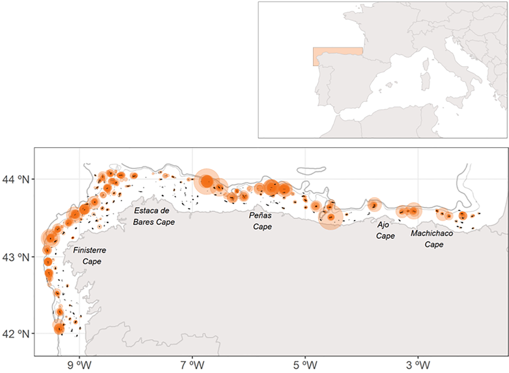
Map of the study area showing the sampling locations of four-spot megrim recruits from 1993 to 2020. Black dots represent all hauls conducted, while bubbles indicate hauls with the number of individuals categorized into four ranges: 1-47,48-94, 95-141 and 142-188. Bathymetric lines mark the 300- and 600-meters depth contours.
Only four-spot megrim recruits, defined as age-0 individuals, were considered in this study. Since the length-age key is estimated annually, this information was used to determine the length range of recruits for each year. Accordingly, age-0 individuals were classified as follows: those ≤8 cm from 1986 to 1998 and from 2004 to 2016, those ≤7 cm from 2017 to 2020, and those ≤9 cm from 1999 to 2003.The total number of individuals caught per 30 minutes trawl was used as abundance index. A presence/absence variable was created for recruits in each haul, where presence was defined as abundance values >0, and absence as abundance equal to 0.
2.2 Environmental variables
Four environmental variables were considered as potential or known predictors of recruit distribution, as they may influence the habitat selection of this species. These include two oceanographic variables: Sea Bottom Temperature (SBT in °C) and Sea Bottom Salinity concentration (SBS in PSU), and two topographic variables: bathymetry (in meters) and type of sediment.
SBT and SBS values were collected during the study with a CTD (conductivity, temperature and depth) device, which was deployed after each fishing haul to gather data throughout the water column. Sediment type was determined through spatial analysis of data obtained with dredges, conducted at sampling points arranged in a grid to comprehensively cover the study area.
As is a standard practice, all covariates were explored for collinearity, outliers, and missing values before being included in the models (Zuur et al., 2010) (see Supplementary Figure S1). Correlation was assessed using Spearman’s correlation, while collinearity was evaluated using Generalized variance-inflation factors (GVIF) (Fox and Weisberg, 2011). To enhance visualization and interpretation, the explanatory variables were standardized by subtracting the mean and dividing by the standard deviation (Gelman, 2008).
2.3 Modelling nursery areas
Exploratory analysis revealed two main characteristics of the four-spot megrim recruit abundance data: strong spatial and temporal dependence and high proportions of zeros since it is absent in a large number of hauls (see Supplementary Figure S2). To address these features, we implemented a hierarchical Bayesian hurdle spatial‐temporal model, which is highly suitable for such data. Indeed, these models account for spatial-temporal autocorrelation, incorporate a component to capture an excess of zeros, and effectively integrate the uncertainties associated to the sampling process (Pennino et al., 2019). In particular, these models combine two types of components: (1) modeling presence/absence to estimate an idea of the relative occurrence of recruits, Yst, and (b) modeling the abundance to approximate the absolute abundance, Zst. For both processes s is the spatial location, and t is the temporal index. As is common in these cases, a Bernoulli distribution was used to model Yst, while a Gamma distribution was applied to model Zst. The latter process depends on the former as follows:
where πst represents the probability of occurrence at location s at time t, and μst and ϕ denote the mean and dispersion of the abundance, respectively. The linear predictors includes: α(Y) and α(Z), which represent the intercepts of each variable; f() a second order random walk (RW2) function to fit non-linear relationships for environmental variables (Fahrmeir and Lang, 2001); g(t) the temporal trend fitted through a RW2 effect over the years; and Ust (Y) and Ust (Z), which represent the spatial-temporal structure of the two processes. Note that the terms g(t) and Ust are shared between both predictors by using the scale parameters η and θ. Three different spatial-temporal structures, namely opportunistic, persistent or progressive, were tested in this study following Paradinas et al., 2017. Opportunistic structures indicate that a species changes the spatial distribution each year without following a specific pattern. On the contrary, persistent structures describe a species with a stable spatial distribution that remains consistent year after year. Finally, progressive structures identify a species that modifies its spatial distribution in a correlated manner from one year to the next. The progressive structure contains an autoregressive parameter, ρt, which controls the level of persistence in the spatial effect. This parameter ranges from 0 to 1, where values close to 0 indicate more opportunistic behaviors, while values close to 1 reflect more persistent distributions over time (Izquierdo et al., 2021).
2.4 Bayesian inference
Following Bayesian reasoning, the parameters are treated as random variables, and prior knowledge must be incorporated through corresponding prior distributions. In particular, a vague zero‐mean Gaussian prior distribution with a variance of 100 was assigned to all of the parameters involved in the fixed effects. For the hyperparameters of the spatial terms and the ρ parameters of the RW2 functions, PC priors (Fuglstad et al., 2018) were used to describe prior knowledge. Following Izquierdo et al., 2021 and Pennino et al., 2022, who implemented similar models for other species in the same area of study, these priors were set as follows: if the prior probability of the spatial range was smaller than 0.5, it was set at 0.05, if the probability of the spatial variance was larger than 0.6, it was also set at 0.05, and if the probability that the precision of the RW2 effects was larger than 0.5, it was set at 0.01.
Inference was performed using the integrated nested Laplace approximation (INLA) methodology (Rue et al., 2009) and software in R (R Development Core Team, 2022).
2.5 Model selection
Model selection was based on two different measures: (a) the Watanabe‐Akaike information criterion (WAIC) (Watanabe, 2010) and Log-Conditional Predictive Ordinates (LCPO) (Roos and Held, 2011). A lower WAIC value indicated a better fit, while LCPO assessed the model’s predictive power, with lower values representing better predictive performance.
Model selection was performed as a subsequently process: (1) testing all the environmental variables to determine whether they should be shared or not shared between the occurrence and abundance processes.; (2) the best model (based on the lower WAIC and LCPO) was used to evaluate the three spatial-temporal structures (i.e., opportunistic, persistent and progressive) Using the best model (based on the lowest WAIC and LCPO values) to evaluate the three spatiotemporal structures (i.e., opportunistic, persistent, and progressive).; (3) once the spatial-temporal structure was selected, a shared RW2 effect for the year was added to the final model to extract the abundance index.
2.6 Model evaluation
INLA performs an internal cross-validation, which consists on a leave-one-out cross-validation process. This process generates a failure vector for each observation, with values ranging from 0 to 1. A value of 0 indicates that the predictive measure for a particular observation is reliable, whereas a value of 1 indicates it is not reliable (Blangiardo and Cameletti, 2015).
2.7 Current stock assessment model
This stock is assessed with assessment for all - a4a (Millar and Jardim, 2019), a non-linear catch-at-age model implemented in R (R Core Team, 2022) and FLR framework (Kell et al., 2007). The model is run using ADMB (Fournier et al., 2012), allowing for rapid application with low parameterization requirements (ICES, 2024). The model is composed of five sub-models, each based on different structural assumptions. The first sub-model addresses fishing mortality at age, where age is treated as a factor, with any ages greater than 6 being capped at 6, and year is also considered as a factor. The second sub-model defines the initial age structure, where age is again treated as a factor. The third sub-model focuses on recruitment, with year as a factor, and fishing mortality is freely estimated for each year. The fourth sub-model involves a list of models for abundance indices and catchability-at-age, where catchability is modeled using a logistic function. Finally, the fifth sub-model models the observation variance of catch-at-age and abundance indices, using the default value of the a4aSCA function.
An FLStock object is required as input data. This object includes various components such as catches, (landings and discards), weights-at-age, natural mortality (M), maturity, harvest before spawning and mortality (ICES, 2024). The commercial catch data (comprising international catches, ages, and length frequencies from catch sampling) are available for Spain and Portugal from 1986 to 2022. Two survey indices are provided: the Spanish SP-NSGFSQ4 (1988 - 2022) and the Portuguese NepS (FU 2829) (1997 - 2018). The maturity ogive is assumed to be constant and natural mortality is set to a value of 0.2 (ICES, 2023).
3 Results
3.1 Spatial modelling results
Out of 3328 samples collected in the study area, four-spot megrim recruits were present in 674 of these stations. The total abundance recorded per sample ranged from a minimum of 0 to a maximum of 188 individuals.
According to the model selection scores (Table 1), the occurrence and abundance distributions of four-spot megrim recruits were mainly influenced by the bathymetry variable. This effect of bathymetry was most pronounced when it was not shared between the occurrence and abundance processes, suggesting that their bathymetric ranges differ. Models that treated bathymetry as not shared effect for occurrence and abundance, recorded a lower WAIC and LPCO compared to the others (Table 1). Among the different spatio-temporal structures, the progressive structure had the one the lowest WAIC and LPCO values (Table 1).
Table 1
| Model | WAIC | LCPO | Failure |
|---|---|---|---|
| Bathymetry shared | 6445.65 | 0.79 | 0 |
| Bathymetry not shared | 6426.15 | 0.78 | 0 |
| SSS shared | 7688.83 | 0.90 | 0 |
| SSS not shared | 7691.54 | 0.90 | 0 |
| SST shared | 7491.52 | 0.88 | 1 |
| SST not shared | 7489.18 | 0.88 | 1 |
| Type of sediment shared | 7678.47 | 0.90 | 0 |
| Type of sediment not shared | 7675.15 | 0.90 | 0 |
| progressive | 5816.03 | 0.76 | 0 |
| opportunistic | 7688.83 | 0.79 | 0 |
| persistent | 7491.52 | 0.90 | 0 |
Comparison of the main four-spot megrim models based on WAIC and LCPO scores and the failure vector.
Since bathymetry was the only relevant variable included in the final model, the original scale units were used to facilitate interpretation of its partial effect. Figure 2 shows that there is an optimal bathymetric range between 150 and 300 m for both the occurrence and abundance of four-spot megrim recruits, with abundance gradually decreasing in deeper waters.
Figure 2
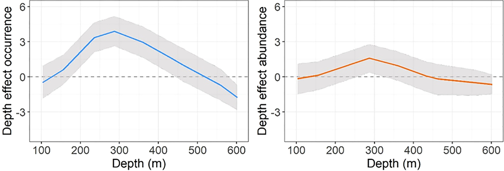
Smoothed (RW2) depth effects predicted for the occurrence and abundance of four-spot megrim on the linear predictor log-scale. Shaded regions represent the approximate 95% credibility interval.
Although the spatio-temporal structure was selected, the temporal correlation parameter in the final model was close to 1 in both processes (0.97 for the occurrence and 0.96 for abundance process). This suggest that while recruits change their distribution in space, these changes are highly correlated between years.
The temporal trend of the year smoothed effect for four-spot megrim abundance shows a clear pattern of change over time, with the abundance of recruits varying considerably throughout the entire time series (Figure 3). The same trend is observed in the year effect for four-spot megrim occurrence (see Supplementary Figure S3).
Figure 3
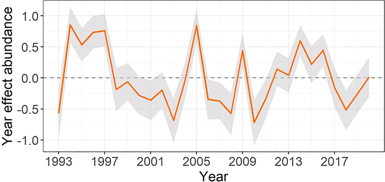
Smoothed (RW2) year effect predicted for the abundance of four-spot megrim on the linear predictor log-scale. Shaded regions represent the approximate 95% credibility interval. Note that the year term is shared in both predictors (occurrence and abundance) by the scale parameter η = 0.86.
To better identify the main abundance hot-spots areas throughout the entire time-series, four time-steps were averaged (Figure 4). The mean of the posterior distributions of the spatial effects reveals a clear increasing pattern in the abundance of the species in the western part of the Iberian Peninsula from 1993 to 2020 (Figure 4). Indeed, from the begging of the time series, there appears to have been shift in the distribution from the eastern part of the study area (Cantabrian Sea) to the western one (Figure 4). The standard deviation (sd) of the posterior distributions of the spatial effects remained consistent over the study period (see Supplementary Figure S4). It is also important to note that since the spatio-temporal structure is shared between the occurrence and abundance processes, the spatial effect is the same for both cases (Supplementary Figure S5).
Figure 4
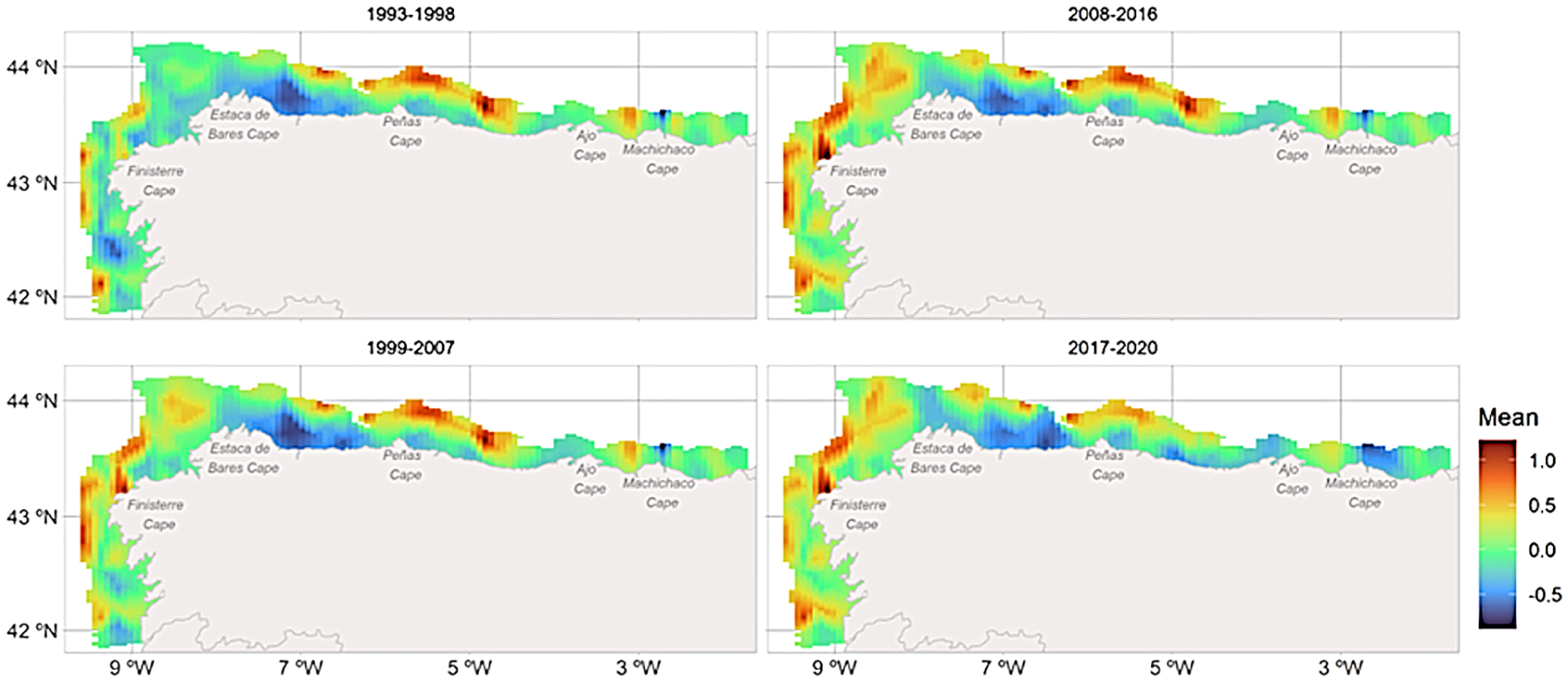
Spatio-temporal mean posterior distribution maps for the abundance of the four-spot megrim grouped by year steps. Cold colors represent areas of low abundance whereas warm colors indicate areas where abundance is high. Note that the spatio-temporal term is shared in both predictors (occurrence and abundance) by the scale parameter θ=0.47.
Overall, four hotspots were identified. The main hotspot (1) is located north of Peñas Cape, where high abundance was observed throughout most of the time series, with a slight decrease noted in the final years. A similar pattern was seen in the smaller hotspot (2) located in the northeast near Ajo Cape. Another important hotspot (3) appeared in the northwest of Estaca de Bares cape (off La Coruña), displaying almost no abundance from 1993 to 1998, followed by a steady increase through 2017-2020. A small hotspot (4) was also found in deeper waters to the southwest of Finisterre Cape (off Vigo), where it was present in the first two time-periods but gradually increased and moved closer to the coast over the past two decades. These shifts demonstrate a progressive movement of the spatial abundance hot-spots throughout the time series (Supplementary Figures S6A–C).
3.2 Spatial approach in single stock assessment results
The results indicate that the study area is divided into two zones with different dynamics concerning the nursery areas over time. As a first step, an attempt has been made to include this spatial information into the assessment model. The nurseries in the Cantabrian area tends to remain stable, with a slight decline in abundance over time, while those in the Galicia area show a progressive increase. The abundance index, expressed in number of individuals per age in the survey, is used to calibrate the model. This index is particularly effective precisely for younger stock ages, including the recruitment age (ICES, 2024). Since this index represents the total area of distribution of the species in the study area and is stratified, a preliminary approach involves dividing it into the two defined zones (Figure 5) to incorporate the spatial effect, reflecting the strength of recruitment by area.
Figure 5
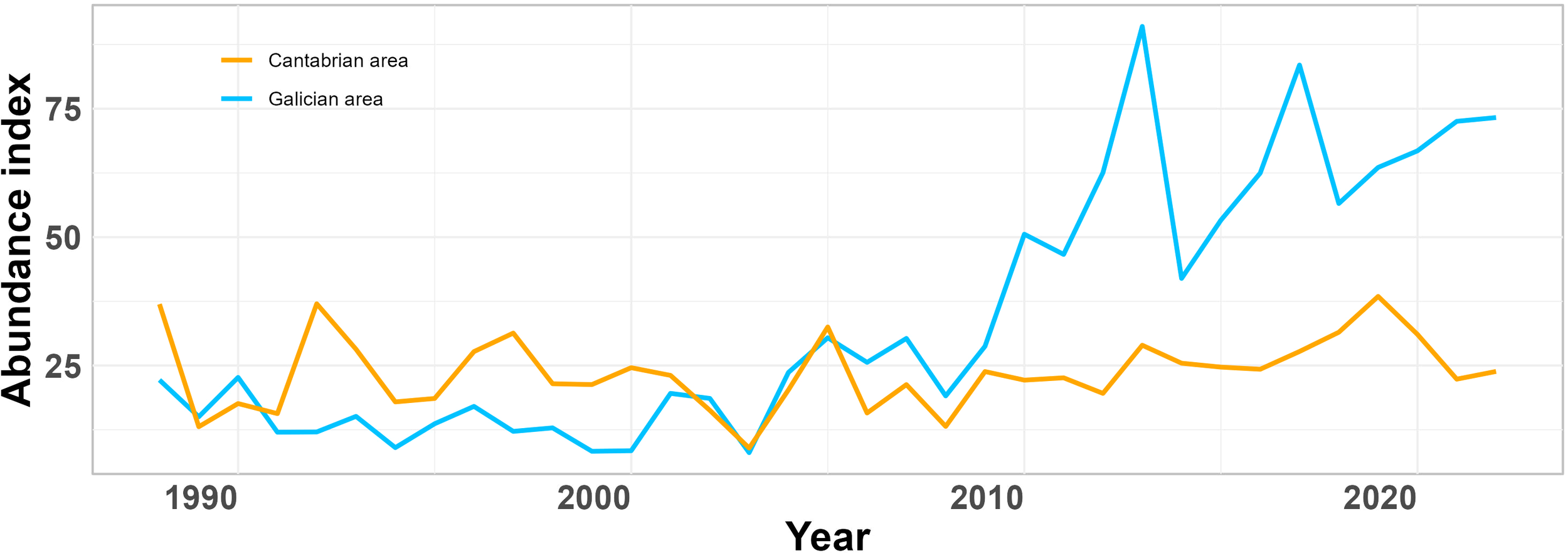
Abundance indices (number of individuals/30 minutes) from SP-NSGFSQ4 survey. Orange line is Cantabrian area and blue line is Galician area.
This variation in the model input data in the current assessment model does not result in significant changes in the model outcomes of Spawning stock biomass and Fishing mortality compared to those previously (Supplementary Figure S7). However, when recalculating the biological reference points (BRPs) of the stock following the ICES procedure (ICES, 2024), differences are observed (Table 2). These differences are evident when comparing the current values to those obtained in this study. For example, the MSY Btrigger has decreased from 3375 t in the study to 2932 t in the current values, indicating a slight reduction in the threshold below which the stock may face a low probability of sustainable exploitation. Similarly, the FMSY, which represents the fishing pressure that maximizes sustainable yield, shows a small decrease from 0.194 in the study to 0.176 in the current model, suggesting a slightly lower optimal fishing mortality rate. Lastly, the Blim, the spawning stock biomass threshold below which reproductive capacity could be reduced, has also decreased from 2672 t in the study to 2321 t in the current values. These recalculated values, while reflecting a similar trend, suggest that the updated spatial data or input parameters may lead to more conservative reference points, potentially affecting future stock management strategies.
Table 2
| BRP | Definition | This study values | Current values |
|---|---|---|---|
| MSY Btrigger | A low biomass that is encountered with a low probability if a stock is exploited at FMSY | 3375 t | 2932 t |
| FMSY | Fishing pressure that gives the maximum sustainable yield in the long term | 0.194 | 0.176 |
| Blim | Spawning stock biomass below which there may be reduced reproductive capacity | 2672 t | 2321 t |
Comparison of biological reference points.
Current values refer to the ones used in the official stock assessment in ICES.
4 Discussion
In this study, we aimed to identify a methodology for locating the nursery areas of the four-spot megrim and assessing their persistence in space and time. These areas are essential for maintaining a healthy population and for managing the resource to ensure its sustainability (Paradinas et al., 2015). Additionally, this methodology provides valuable spatial information that, when included in the stock assessment model, enhances the precision of the results used to inform scientific advice on recommended catch levels for the stock (Punt, 2019; Booth, 2000). The findings of this study are inherently constrained by the temporal scope of the annual oceanographic survey. However, this time frame offers a valuable opportunity to examine annual recruitment dynamics, as the majority of spawning occurs in April, enabling the effective capture of zero-age individuals using the employed fishing gear.
An important challenge with this species is that mature individuals do not migrate to shallow areas for reproduction, resulting in a significant gap in biological knowledge in the spawning areas and early life stages dispersion that results in the spatiotemporal variability observed in the nursery areas. The inability to study the development of eggs and larvae under laboratory conditions further challenge our capacity to understand drifting pathways and survival of early life stages. In contrast, other flatfish species are influenced by variables such as temperature regimes (Dunlop et al., 2022) and high freshwater inflows during the spawning season, which are important for recruitment success, as they occur in coastal or estuarine areas (Morrongiello et al., 2014).
The distributions of occurrence and abundance for four-spot megrim recruits were primarily influenced by the bathymetry variable. This influence is most effective when the occurrence and abundance processes do not share the same bathymetric range, suggesting that these processes driving occupancy and strength on aggregations have a different bathymetric preference. The optimal bathymetric range for the occurrence and abundance for four-spot megrim recruits lies between 150 and 300 meters, which is consistent with the species’ known bathymetric preference (Fernández-Zapico et al, 2017; Sánchez et al, 1998). This range also aligns with findings from another study on undersized four-spot megrim (individuals smaller than 20 cm), whose preferred habitat spans from 100 to 350 meters (Abad et al., 2020). In that study, the abundance of these undersized four-spot megrims was primarily explained by depth, thought other factors such as SBT, SBS and spatial and temporal effects also played a role (Abad et al., 2020). As a species that reproduces in deep waters, it is logical that bathymetry emerges as a key variable influencing the distribution of recruits and the location of nurseries, as demonstrated in previous studies (Izquierdo et al., 2021).
For both occurrence and recruit abundance, the results revealed a significant variability throughout the time series. The predicted trend observed in the graph aligns with the recruitment values obtained from the model used to assess this stock, showing consistency in the peaks of recruit abundance (ICES, 2024). It is well known that recruitment is a highly dynamic process, with external factors from local to regional scale playing a crucial role in determining success or failure, which explains its high variability (Hidalgo et al., 2019; Zimmermann et al., 2019; Duffy-Anderson et al., 2005; Cardinale and Arrhenius, 2000). Therefore, a more comprehensive investigation of habitats is necessary, incorporating additional variables known to significantly affect the distribution of individuals in other flatfish species. These include mesoscale and hydrodynamic processes that play critical roles in larval dispersal (Barbut et al., 2019), along with a better description of the static properties of the substrate of the preferred nursery areas and how they are connected among populations subunits. While our model identifies spatiotemporal variations in nursery areas, it is important to acknowledge that the limited number of variables included in the analysis may not fully capture all factors influencing recruits distribution. Future studies should explore additional environmental and ecological variables, as well as potential interactions between them, to better understand the drivers of these spatial changes.
The spatiotemporal analysis of nurseries revealed four well-defined hotspots within the study area and timeframe. These hotspots align with those identified in previous research on the distribution of commercially sized and undersized individuals of this species (Abad et al., 2020). Overlap was observed, particularly in the case of undersized individuals, as these hotspots also encompass age-zero recruits, along with some areas where commercial-sized and fully mature individuals are present. Thus, a spatial ban on nurseries would not only protect the recruits but also provide protection for a portion of the spawners, offering dual benefit for the population. A different temporal dynamic of the hotspot groups emerged in our analyses, where the two located in the eastern area appear stable over time with a decrease at the end of the period while the two in the western area show an upward trend, with a notable increase in the last period, are key factors for consideration in fishery management. This spatial and abundance shift highlights the importance of adopting dynamic and adaptive stock management strategies, which have been advocated in several studies as a means to achieve more effective and sustainable exploitation in the long term. Given this significance, future research could benefit from complementing the analyzed approach with mechanistic studies aimed at explaining the specific causes of these spatial changes. Furthermore, during the implementation of the landing obligation, it was emphasized that minimizing discards by avoiding high-discard areas benefits both the resource and the fishing industry (Guillen et al., 2018). Management measures informed by updated spatial data, such as temporary spatial closures, could play a significant role in preserving exploited populations. These measures ensure their sustainability while supporting the economic viability of fisheries, as dynamic scenarios may require fewer permanently closed areas compared to traditional closures (Vigo et al., 2024). Since improving protection is easier than increasing productivity, priority areas for protection should be those with high connectivity, as these are crucial to sustain an efficient pathway between the spawners spawning areas and the nurseries. By integrating population dynamics and fishing effort into a spatiotemporal model, area-based fisheries management tools could be effectively evaluated (Radici et al., 2023; Booth, 2000).
Despite the growing understanding of the importance of spatial information in the dynamics of exploited populations, it is currently not incorporated into almost any stock assessment model used by the major international scientific organizations dedicated to providing advice. While spatial structure is crucial in population assessments, models that integrate this information generally perform better. These models present new challenges and proposals that differ from traditional approaches and their application in fisheries management remain limited, particularly their extensive data requirements including knowledge the spatial populations structure and rates of subunits exchange movement and directions (Cadrin et al., 2020). However, in the last years several spatially explicit stock assessment models have been developed (e.g. Goethel et al., 2015; Cao et al., 2020; Thorson et al., 2021), along with good practices and recommendations opening a realistic platform for a future and more widespread implementation (Goethel et al., 2023).
Incorporating spatial structure into stock assessments with precision can enhance model accuracy, reduce the risk of misinterpreting stock status, and help avoid shortcomings in fisheries management (Cadrin, 2020; Goethel et al., 2023). The stock of four-spot megrim in the Atlantic region of the Iberian Peninsula is assessed using the a4a model. While this model does not directly incorporate spatial information, it is important to evaluate how such information could impact the results of the stock assessment. Specifically, analyzing the influence of varying trends in recruitment hotspots across the two different areas is crucial. This analysis could incorporate spatial effects into future management measures or lead to the proposal of more efficient alternative. In addition, future studies can also explore influence of the rates of exchange and direction between putative population subunits of the species.
The incorporation of spatial information into the model, in the form of two different abundance indices based on the area, yielded different results. When comparing the results from the assessment model used annually with those that included these two indices, the differences are not significant. However, a slight increase was observed in some values, such as fishing mortality (F) and the biomass of the spawning stock (SSB) in the assessment year. Despite this, these changes did not result in a substantial shift in the annual advice on recommended catches for the stock. However, recalculating the biological reference points (BRPs) of the stock revealed differences in the values, showing an upward trend in Blim, FMSY and MSY Btrigger, which affect management measures. Previous studies have shown that failing to incorporate the correct spatial structure when calculating BRPs can lead to biased stock status indicators, overexploitation or missed opportunities for designing management measures that optimize performance (Goethel and Berger, 2017; Goethel et al., 2024). Furthermore, changes driven by climatic variations that affect productivity—and consequently, BRPs based on long-term fish stock productivity (O’Leary et al., 2020)—highlight the importance of continually improving stock assessment models. These improvements will contribute to more accurate harvest control rules and more effective fisheries management.
Statements
Data availability statement
The raw data supporting the conclusions of this article will be made available by the authors, without undue reservation.
Ethics statement
The manuscript presents research on animals that do not require ethical approval for their study.
Author contributions
EA: Conceptualization, Data curation, Formal analysis, Investigation, Methodology, Resources, Writing – original draft, Writing – review & editing. FI: Conceptualization, Data curation, Formal analysis, Investigation, Methodology, Resources, Writing – original draft, Writing – review & editing. JL: Data curation, Investigation, Resources, Writing – review & editing. FV: Data curation, Investigation, Resources, Writing – review & editing. MH: Conceptualization, Funding acquisition, Investigation, Project administration, Resources, Supervision, Writing – review & editing. MP: Conceptualization, Funding acquisition, Investigation, Methodology, Project administration, Resources, Supervision, Writing – original draft, Writing – review & editing.
Funding
The author(s) declare that financial support was received for the research and/or publication of this article. The authors thank the funding for the following projects in the different sections of this study: National Program of collection, management and use of data in the fisheries sector and support for scientific advice regarding the Common Fisheries Policy, co-funded by the European Union through the European Maritime Fisheries and Aquaculture Fund (EMFAF), COCOCHA research project Grant PID2019-110282RA-100 funded by MCIN/AEI/10.13039/501100011033, FRESCO research project PID2022-140290OB-I00 funded by MCIN/AEI/10.13039/501100011033/and by “ERDF A way of making Europe”, Ministry of Science, Innovation and Universities—State Research Agency.
Conflict of interest
The authors declare that the research was conducted in the absence of any commercial or financial relationships that could be construed as a potential conflict of interest.
Generative AI statement
The author(s) declare that no Generative AI was used in the creation of this manuscript.
Publisher’s note
All claims expressed in this article are solely those of the authors and do not necessarily represent those of their affiliated organizations, or those of the publisher, the editors and the reviewers. Any product that may be evaluated in this article, or claim that may be made by its manufacturer, is not guaranteed or endorsed by the publisher.
Supplementary material
The Supplementary Material for this article can be found online at: https://www.frontiersin.org/articles/10.3389/fmars.2025.1545819/full#supplementary-material
Supplementary Figure 1Smoothed relationships and correlation between the response variable and the environmental covariates.
Supplementary Figure 2Number of sampling hauls by year where the four-spot megrim was present and absent.
Supplementary Figure 3Smoothed (RW2) year shared effect predicted for the occurrence of four-spot megrim on the linear predictor log-scale. Shaded regions represent the approximate 95% credibility interval. Note that the year term is shared in both predictors (occurrence and abundance) by the scale parameter η = 1.088.
Supplementary Figure 4Spatio-temporal mean posterior distribution maps for occurrence of four-spot megrim grouped by year steps. Cold colors represent areas of low presence whereas warm colors indicate areas where presence is high. Note that the spatio-temporal term is shared in both predictors (occurrence and abundance) by the scale parameter θ=0.627.
Supplementary Figure 5Spatio-temporal standard deviation (sd) posterior distribution maps for the occurrence and abundance of four-spot megrim grouped by year steps. Cold colors represent areas of low uncertainty whereas warm colors indicate areas where uncertainty is high.
Supplementary Figure 6(A) Spatio-temporal mean posterior distribution maps for the abundance of four-spot megrim by year. Cold colors represent areas of low abundance whereas warm colors indicate areas where abundance is high. Note that the spatio-temporal term is shared in both predictors (occurrence and abundance) by the scale parameter θ=0.627. (B) Spatio-temporal mean posterior distribution maps for the abundance of four-spot megrim by year. Cold colors represent areas of low abundance whereas warm colors indicate areas where abundance is high. Note that the spatio-temporal term is shared in both predictors (occurrence and abundance) by the scale parameter θ=0.627. (C) Spatio-temporal mean posterior distribution maps for the abundance of four-spot megrim by year. Cold colors represent areas of low abundance whereas warm colors indicate areas where abundance is high. Note that the spatio-temporal term is shared in both predictors (occurrence and abundance) by the scale parameter θ=0.627.
Supplementary Figure 7Comparative results of the assessment models for Spawning stock biomass and for fishing mortality. Orange lines are the results of this study and blue lines are the results of the current assessment in ICES.
References
1
Abad E. Pennino M. Valeiras J. Vílela R. Bellido J. Punzón A. et al . (2020). Integrating spatial management measures into fisheries: The Lepidorhombus spp. case study. Mar. Policy116, 103739. doi: 10.1016/j.marpol.2019.103739
2
Barbut L. Crego C. Delerue-Ricard S. Vandamme S. Volckaert F. Lacroix G. (2019). How larval traits of six flatfish species impact connectivity. Limnol. Oceanogr.64 (3), 1150–1171. doi: 10.1002/lno.11104
3
Blangiardo M. Cameletti M. . (2015). Spatial and Spatio-Temporal Bayesian Models with R-INLA. New York: John Wiley and Sons Inc..
4
Booth A. (2000). Incorporating the spatial component of fisheries data into stock assessment models. J. Mater. Sci.57, 858–865. doi: 10.1006/JMSC.2000.0816
5
Cadrin S. (2020). Defining spatial structure for fishery stock assessment. Fish. Res. 221, 105397. doi: 10.1016/j.fishres.2019.105397
6
Cadrin S. Maunder M. Punt A. (2020). Spatial Structure: Theory, estimation and application in stock assessment models. Fish. Res.229, 105608. doi: 10.1016/j.fishres.2020.105608
7
Cao J. Thorson J. T. Punt A. E. Szuwalski C. (2020). A novel spatiotemporal stock assessment framework to better address fine-scale species distributions: Development and simulation testing. Fish Fish.21, 350–367. doi: 10.1111/faf.12433
8
Cardinale M. Arrhenius F. (2000). The influence of stock structure and environmental conditions on the recruitment process of Baltic cod estimated using a generalized additive model. Can. J. Fish. Aquat. Sci.57, 2402–2409. doi: 10.1139/F00-221
9
Cecino G. Valavi R. Treml E. (2021). Testing the influence of seascape connectivity on marine-based species distribution models. Frontiers in Marine Science, 8, 766915. doi: 10.3389/fmars.2021.766915
10
Colloca F. Bartolino V. Lasinio G. Maiorano L. Sartor P. Ardizzone G. (2009). Identifying fish nurseries using density and persistence measures. Mar. Ecol. Prog. Ser.381, 287–296. doi: 10.3354/MEPS07942
11
Colloca F. Garofalo G. Bitetto I. Facchini M. Grati F. Martiradonna A. et al . (2015). The seascape of demersal fish nursery areas in the North Mediterranean Sea, a first step towards the implementation of spatial planning for trawl fisheries. PloS One10 (3), e0119590. doi: 10.1371/journal.pone.0119590
12
Duffy-Anderson J. Bailey K. Ciannelli L. Cury P. Belgrano A. Stenseth N. (2005). Phase transitions in marine fish recruitment processes. Ecol. Complexity2, 205–218. doi: 10.1016/J.ECOCOM.2004.12.002
13
Dunlop K. Staby A. van der Meeren T. Keeley N. Olsen E. M. Bannister R. et al . (2022). Habitat associations of juvenile Atlantic cod (Gadus morhua L.) and sympatric demersal fish communities within shallow inshore nursery grounds. Estuar. Coast. Shelf Sci.279, 108111. doi: 10.1016/j.ecss.2022.108111
14
European Parliament and Council . (2013). Regulation (EU) No 1380/2013 of the European Parliament and of the Council of 11 December 2013 on the Common Fisheries Policy. Official Journal of the European Union, L 354/22. https://eur-lex.europa.eu/legal-content/EN/TXT/?uri=CELEX%3A32013R1380
15
Fahrmeir L. Lang S. (2001). Bayesian semiparametric regression analysis of multicategorical time-space data. Ann. Inst. Stat. Math.53, 11–30. doi: 10.1023/A:1017904118167
16
Fernández-Zapico O. Punzón A. Serrano A. Landa J. Ruiz-Pico S. Velasco F. (2017). Environmental drivers of the distribution of the order Pleuronectiformes in the Northern Spanish Shelf. J. Sea Res.130, 217–228. doi: 10.1016/J.SEARES.2017.02.013
17
Florin A. Sundblad G. Bergström U. (2009). Characterisation of juvenile flatfish habitats in the Baltic Sea. Estuar. Coast. Shelf Sci.82, 294–300. doi: 10.1016/J.ECSS.2009.01.012
18
Fournier D. Skaug H. Ancheta J. Ianelli J. Magnusson A. Maunder M. et al . (2012). AD Model Builder: using automatic differentiation for statistical inference of highly parameterized complex nonlinear models. Optimization Methods Softw.27, 233–249. doi: 10.1080/10556788.2011.597854
19
Fox J. Weisberg S. (2011). CAR: Companion to Applied Regression. Available online at: http://cran.R-project.org/package=car (Accessed April 12, 2023).
20
Fuglstad G. A. Simpson D. Lindgren F. Rue H. (2018). Constructing priors that penalize the complexity of gaussian random fields. J. Am. Stat. Assoc.114, 445–452. doi: 10.1080/01621459.2017.1415907
21
Gelman A. (2008). Scaling regression inputs by dividing by two standard deviations. Stat Med.27, 2865–2873. doi: 10.1002/sim.3107
22
Goethel D. Berger A. (2017). Accounting for spatial complexities in the calculation of biological reference points: effects of misdiagnosing population structure for stock status indicators. Can. J. Fish. Aquat. Sci.74, 1878–1894. doi: 10.1139/CJFAS-2016-0290
23
Goethel D. Berger A. Hoyle S. Lynch P. Barceló C. Deroba J. et al . (2024). ‘Drivin’ with your eyes closed’: Results from an international, blinded simulation experiment to evaluate spatial stock assessments. Fish Fish.25 (3), 471–490. doi: 10.1111/faf.12819
24
Goethel D. R. Berger A. M. Cadrin S. X. (2023). Spatial awareness: Good practices and pragmatic recommendations for developing spatially structured stock assessments. Fish. Res.264, 106703. doi: 10.1016/j.fishres.2023.106703
25
Goethel D. R. Legault C. M. Cadrin S. X. (2015). Demonstration of a spatially explicit, tag-integrated stock assessment model with application to three interconnected stocks of yellowtail flounder off of New England. ICES J. Mar. Sci.72, 164–177. doi: 10.1093/icesjms/fsu014
26
Guillen J. Holmes S. Carvalho N. Casey J. Dörner H. Gibin M. et al . (2018). A review of the European Union landing obligation focusing on its implications for fisheries and the environment. Sustainability10, 900. doi: 10.3390/SU10040900
27
Hidalgo M. Rossi V. Monroy P. Ser-Giacomi E. Hernández-García E. Guijarro B. et al . (2019). Accounting for ocean connectivity and hydroclimate in fish recruitment fluctuations within transboundary metapopulations. Ecol. Applications: Publ. Ecol. Soc. America29, e01913. doi: 10.1002/eap.1913
28
ICES (2017). Manual of the IBTS North Eastern Atlantic Surveys. Series of ICES Survey Protocols SISP 15 (Copenhagen: ICES).
29
ICES (2023). “Four-spot megrim (Lepidorhombus boscii) in divisions 8.c and 9.a (southern Bay of Biscay and Atlantic Iberian waters East). (southern Bay of Biscay and Atlantic Iberian waters East). ICES Advice: Recurrent Advice. Report. doi: 10.17895/ices.advice.21840912.v1
30
ICES (2024). “Working group for the Bay of Biscay and the Iberian waters ecoregion (WGBIE),” in ICES Scientific Reports, vol. 6, 762 pp. doi: 10.17895/ices.pub.25908130
31
Izquierdo F. Paradinas I. Cerviño S. Conesa D. Alonso-Fernández A. Velasco F. et al . (2021). Spatio-temporal assessment of the European hake (Merluccius merluccius) Recruits in the Northern Iberian Peninsula. Front. Mar. Sci.8, 614675. doi: 10.3389/fmars.2021.614675
32
Kell L. Mosqueira I. Grosjean P. Fromentin J. Garcia D. Hillary R. et al . (2007). FLR: an open-source framework for the evaluation and development of management strategies. Ices J. Mar. Sci.64, 640–646. doi: 10.1093/ICESJMS/FSM012
33
Kerametsidis G. Thorson J. Rossi V. Álvarez-Berastegui D. Barnes C. Certain G. et al . (2024). Cross-scale environmental impacts across persistent and dynamic aggregations within a complex population: implications for fisheries management. Can. J. Fish. Aquat. Sci.81 (3), 268–284. doi: 10.1139/cjfas-2023-0120
34
Landa J. Fontenla J. (2016). Age and growth of four spot megrim (Lepidorhombus boscii) in northern Iberian waters corroborated by cohort tracking. Estuar. Coast. Shelf Sci.179, 181–188. doi: 10.1016/J.ECSS.2016.01.010
35
Millar C. Jardim E. (2019). a4a: A flexible and robust stock assessment framework. R package version 1.8.2. Available online at: https://flr-project.org/FLa4a/ (Accessed February 2, 2024).
36
Morrongiello J. Walsh C. Gray C. Stocks J. Crook D. (2014). Environmental change drives long-term recruitment and growth variation in an estuarine fish. Global Change Biol.20 (6), 1844–1860. doi: 10.1111/gcb.12545
37
O’Leary C. Thorson J. Miller T. Nye J. (2020). Comparison of multiple approaches to calculate time-varying biological reference points in climate-linked population-dynamics models. Ices J. Mar. Sci.77, 930–941. doi: 10.1093/icesjms/fsz215
38
Paradinas I. Conesa D. López-Quílez A. Bellido J. M. (2017). Spatio-temporal model structures with shared components for semi-continuous species distribution modelling. Spat. Stat.22, 434–450. doi: 10.1016/j.spasta.2017.08.001
39
Paradinas I. Conesa D. Pennino M. Muñoz F. Fernández Á. López-Quílez A. et al . (2015). Bayesian spatio-temporal approach to identifying fish nurseries by validating persistence areas. Mar. Ecol. Prog. Ser.528, 245–255. doi: 10.3354/MEPS11281
40
Pennino M. G. Vilela R. Bellido J. M. Velasco F. (2019). Balancing resource protection and fishing activity: The case of the European hake in the northern Iberian Peninsula. Fish. Oceanogr.28 (1), 54–65.
41
Pennino M. G. Izquierdo F. Paradinas I. Cousido M. Velasco F. Cerviño S. (2022). Identifying persistent biomass areas: The case study of the common sole in the northern Iberian waters. Fish. Res.248, 106196. doi: 10.1016/j.fishres.2021.106196
42
Punt A. (2019). Spatial stock assessment methods: A viewpoint on current issues and assumptions. Fish. Res. 213, 132–143. doi: 10.1016/J.FISHRES.2019.01.014
43
Punzón A. Hernández C. Abad E. Castro J. Pérez N. Trujillo V. (2010). Spanish otter trawl fisheries in the Cantabrian Sea. ICES J. Mar. Sci.67, 1604–1616. doi: 10.1093/icesjms/fsq085
44
Radici A. Claudet J. Ligas A. Bitetto I. Lembo G. Spedicato M. et al . (2023). Assessing fish–fishery dynamics from a spatially explicit metapopulation perspective reveals winners and losers in fisheries management. J. Appl. Ecol. 60 (11), 2482–2493. doi: 10.1111/1365-2664.14508
45
R Development Core Team (2022). R: A Language and Environment for Statistical Computing (R Foundation for Statistical Computing). Available at: https://www.r-project.org (Accessed April 12, 2023).
46
Roos M. Held L. (2011). Sensitivity analysis in Bayesian generalized linear mixed models for binary data. Bayesian Anal.6, 259–278. doi: 10.1214/11-BA609
47
Roos N. Longo G. Pennino M. Francini-Filho R. Carvalho A. (2020). Protecting nursery areas without fisheries management is not enough to conserve the most endangered parrotfish of the Atlantic Ocean. Sci. Rep.10, 19143. doi: 10.1038/s41598-020-76207-x
48
Rue H. Martino S. Chopin N. (2009). Approximate Bayesian inference for latent Gaussian models by using integrated nested Laplace approximations. J. R. Stat. Soc B.71, 319–392. doi: 10.1111/j.1467-9868.2008.00700.x
49
Sánchez F. Pérez N. Landa J. (1998). Distribution and abundance of megrim (Lepidorhombus boscii and Lepidorhombus whiffiagonis) on the northern Spanish shelf. ICES J. Mar. Sci.55 (3), 494–514. doi: 10.1006/jmsc.1997.0279
50
Thorson J. T. Barbeaux S. J. Goethel D. R. Kearney K. A. Laman E. A. Nielsen J. K. et al . (2021). Estimating fine-scale movement rates and habitat preferences using multiple data sources. Fish Fish.22, 1359–1376. doi: 10.1111/faf.12592
51
van der Veer H. W. Tulp I. Witte J. I. J. Poiesz S. S. H. Bolle L. J. (2022). Changes in functioning of the largest coastal North Sea flatfish nursery, the Wadden Sea, over the past half century. Mar. Ecol. Prog. Ser.693, 183–201. doi: 10.3354/meps14082
52
Vigo M. Hermoso V. Navarro J. Sala-Coromina J. Company J. Giakoumi S. (2024). Dynamic marine spatial planning for conservation and fisheries benefits. Fish Fish.25 (4), 630–646. doi: 10.1111/faf.12830
53
Watanabe S. (2010). Asymptotic Equivalence of Bayes Cross Validation and Widely Applicable Information Criterion in Singular Learning Theory. ArXivabs/1004.2316. doi: 10.5555/1756006.1953045
54
Wilson M. Mier K. Cooper D. (2016). Assessment of resource selection models to predict occurrence of five juvenile flatfish species (Pleuronectidae) over the continental shelf in the western Gulf of Alaska. J. Sea Res.111, 54–64. doi: 10.1016/J.SEARES.2015.12.005
55
Zimmermann F. Claireaux M. Enberg K. (2019). Common trends in recruitment dynamics of north-east Atlantic fish stocks and their links to environment, ecology and management. Fish Fish.20 (3), 518–536. doi: 10.1111/FAF.12360
56
Zuur A. F. Ieno E. N. Elphick C. S. (2010). A protocol for data exploration to avoid common statistical problems. Methods Ecol. Evol.1, 3e14. doi: 10.1111/j.2041-210X.2009.00001.x
Summary
Keywords
Bayesian models, fisheries management, four-spot megrim, nurseries, spatial assessment, recruits
Citation
Abad E, Izquierdo F, Landa J, Velasco F, Hidalgo M and Pennino MG (2025) Identifying spatiotemporal variations in four-spot megrim (Lepidorhombus boscii) fishery nurseries to enhance management and stock assessment. Front. Mar. Sci. 12:1545819. doi: 10.3389/fmars.2025.1545819
Received
15 December 2024
Accepted
20 March 2025
Published
28 April 2025
Volume
12 - 2025
Edited by
Pablo Presa, University of Vigo, Spain
Reviewed by
Mbaye Tine, Gaston Berger University, Senegal
Oumar Sadio, Institut de Recherche pour le Développement, Senegal
Laura Recasens, Spanish National Research Council (CSIC), Spain
Updates
Copyright
© 2025 Abad, Izquierdo, Landa, Velasco, Hidalgo and Pennino.
This is an open-access article distributed under the terms of the Creative Commons Attribution License (CC BY). The use, distribution or reproduction in other forums is permitted, provided the original author(s) and the copyright owner(s) are credited and that the original publication in this journal is cited, in accordance with accepted academic practice. No use, distribution or reproduction is permitted which does not comply with these terms.
*Correspondence: Esther Abad, esther.abad@ieo.csic.es
†Deceased
Disclaimer
All claims expressed in this article are solely those of the authors and do not necessarily represent those of their affiliated organizations, or those of the publisher, the editors and the reviewers. Any product that may be evaluated in this article or claim that may be made by its manufacturer is not guaranteed or endorsed by the publisher.