Abstract
Introduction:
Global warming and glacier melt are transforming Southern Ocean ecosystems, profoundly affecting phytoplankton dynamics. This study investigates long-term phytoplankton changes in the Amundsen and Cosmonaut Seas, focusing on responses to climate-driven environmental shifts and the influence of the Southern Annular Mode (SAM).
Methods:
We analyzed high-resolution (4 km, monthly averaged) satellite-derived chlorophyll-a (Chla) and net primary productivity (NPP) data from austral summers (2003–2020). Environmental parameters, including sea surface temperature (SST), photosynthetically active radiation (PAR) and wind speed (WS), sea ice concentration (SIC) and mixed layer depth (MLD), were examined to elucidate their roles in driving phytoplankton variability in the Amundsen and Cosmonaut Seas.
Results:
During positive SAM phases, Chla and NPP generally increased across both seas, but local ocean circulation led to divergent subregional trends. North of the Southern Antarctic Circumpolar Front (sACCF) and within the Weddell Gyre, enhanced wind-driven MLD promoted Chla increases. In the northern Ross Gyre, cooling SST and deeper MLD intensified upwelling and nutrient, sustaining Chla growth, while shallower MLD and weaker upwelling in the eastern Ross Gyre reduced Chla. In coastal Amundsen Sea, warming SST facilitated sea ice melt, increasing Chla, whereas cooling SST in the Cosmonaut Sea and Prydz Bay increased SIC, reducing Chla.
Discussion:
This high-resolution analysis highlights the complex interplay of physical and biological drivers in polar marine ecosystems, providing critical insights into climate change impacts on Southern Ocean phytoplankton dynamics and their regional variability.
1 Introduction
The elevated atmospheric carbon dioxide (CO2) concentrations have intensified global warming, significantly impacting marine ecosystems by altering ocean circulation, accelerating sea ice melting, and causing ocean acidification (Deppeler and Davidson, 2017; Le Quéré et al., 2016). The Southern Ocean is pivotal in mitigating climate change, accounting for approximately 40% of global oceanic CO2 absorption (Frölicher et al., 2015). As the foundation of marine ecosystems, phytoplankton are essential for evaluating ecosystem changes and comprehending the global carbon cycle and its response to climate change. Key indicators of phytoplankton productivity, such as chlorophyll-a concentration (Chla) and net primary productivity (NPP), are pivotal in these assessments (Arrigo et al., 2008).
Recent research employing field observations, remote sensing, models, and reanalysis data have elucidated spatio-temporal patterns of Chla and NPP in the Southern Ocean and their associations with global climate change (Arrigo et al., 2008, 2015; Feng et al., 2022; Pinkerton et al., 2021). From a long-term perspective, Yu et al. (2023) reported an increasing trend in Southern Ocean Chla based on global Chla product results from 1998 to 2020. Thomalla et al. (2023) similarly observed an upward trend in phytoplankton blooms in this region, albeit with regional variations. Noh et al. (2021) highlighted that Chla trends in the western Amundsen-Ross Sea and the D’Urville Sea exhibited contrasting patterns, attributed to differing limiting factors for phytoplankton growth. While numerous investigations have explored large-scale spatio-temporal changes in phytoplankton productivity in the Southern Ocean, further research is essential to understand long-term and high-resolution changes in marginal seas, especially those influenced by local ocean circulation.
The Southern Ocean is recognized as being exceptionally sensitive to climate change, with various regions experiencing impacts from factors such as ocean warming, increased wind speed (WS), iron (Fe) limitation, sea ice melting, and changes in the mixed layer depth (MLD) (Haumann et al., 2020; Marinov et al., 2006; Ryan-Keogh et al., 2023; Thomalla et al., 2023). Wind-driven MLD deepening had been shown to sustain high Chla during austral summer (Carranza and Gille, 2015), while MLD shoaling has been associated with phytoplankton blooms (Briggs et al., 2018). Elevated sea surface temperatures (SST) and increased photosynthetically active radiation (PAR) have accelerated phytoplankton growth but may also suppress productivity by reducing nutrient supply through stratification (Del Castillo et al., 2019; Carranza and Gille, 2015). Kim and Kim (2021) proposed that primary production in high-latitude regions of the Southern Ocean was likely to increase in the future due to the combined effects of warming, light availability, and Fe inputs. Despite numerous studies indicating that limiting factors for phytoplankton growth vary across different regions of the Southern Ocean, the underlying processes driving phytoplankton variability, influenced by external environmental stressors such as ocean circulation and sea ice dynamics, remain complex and require further investigation (Boyd, 2019; Trimborn et al., 2019). Additionally, the relationship between Southern Ocean phytoplankton concentration and climate change remains insufficiently understood.
The Amundsen Sea, situated in the southwest sector of Antarctica, and the Cosmonaut Sea, located in the northeast sector, are two regions with distinct characteristics. Both are influenced by the Southern Antarctic Circumpolar Front (sACCF), the Antarctic Slope Current (ASC), and other regional ocean currents, yet they exhibit markedly different phytoplankton productivity patterns (Arrigo et al., 2015). Specifically, the Amundsen Sea demonstrates higher primary productivity, with the Amundsen Sea polynya (Annual NPP: 105.4 Tg C yr-1, averaged Chla: 2.28 mg m-3) ranking as one of the highest phytoplankton productivity regions in the Southern Ocean (Arrigo et al., 2015). Conversely, the Cosmonaut Sea exhibits lower primary productivity, particularly in Lützow-Holm Bay, which has an annual NPP of 6.7 Tg C yr-1 and a mean chlorophyll-a concentration of 0.17 mg m-3, ranking it among the least productive regions in the Southern Ocean (Arrigo et al., 2015).
The persistent upwelling of warm Circumpolar Deep Water (CDW) has led to the accelerated melting of West Antarctic ice shelves, making the Amundsen Sea one of the most affected regions in the Southern Ocean (Bett et al., 2020). This unique marine environment has garnered substantial attention in research, leading to an extensive body of literature (Azaneu et al., 2023; Haigh et al., 2023; Park et al., 2024; Xie et al., 2024). Pinkerton et al. (2021) utilized multiple linear regression analysis to conclude that SST exerts a more significant influence on the Chla trend in the Amundsen Sea than PAR, MLD, and SIC (sea ice concentration). Furthermore, they highlighted that the spatial resolution and coverage limitations of remote sensing data necessitate further investigation into the spatial variations in phytoplankton productivity and their underlying mechanisms (Pinkerton et al., 2021). Studies on productivity changes in the Cosmonaut Sea have predominantly relied on field observations or large-scale analyses from the South Indian Ocean sector (Schwarz et al., 2010; Takao et al., 2012), rendering it one of the less studied regions of the Southern Ocean. Consequently, a comparative analysis of the marine environments of the Amundsen and Cosmonaut Seas will enhance our understanding of phytoplankton responses to climate change and variability, offering valuable insights into the controlling mechanisms of phytoplankton productivity.
This study concentrates on the Amundsen and Cosmonaut Seas, utilizing high-resolution remote sensing ocean color data from the Southern Ocean at high latitudes. The objective is to more precisely elucidate the regulatory mechanisms governing phytoplankton changes within the context of climate change. First, in-situ Chla and NPP data were gathered to validate the accuracy of satellite products. Then, long-term temporal variations in satellite products were analyzed and combined with various satellite environmental parameters, and the similarities and differences in phytoplankton changes in the Amundsen and Cosmonaut Seas were explored. This analysis aimed to investigate the similarities and differences in phytoplankton dynamics between the Amundsen and Cosmonaut Seas. Ultimately, through comparative analysis, this study seeks to enhance our understanding of how phytoplankton respond to climate change.
2 Materials and methods
2.1 Study areas
The Amundsen Sea is situated south of 60°S, extending between 160°W and 80°W (Figure 1a). The ocean circulation in this region exhibits considerable complexity, primarily comprising the Ross Gyre, sACCF, and the Antarctic Slope Current (ASC). The interactions among these currents are pivotal to the functioning of the regional marine ecosystem. Notably, the intrusion of warm CDW has altered sea ice distribution and influenced ocean circulation by supplying iron, thereby promoting phytoplankton growth (Bett et al., 2020).
Figure 1
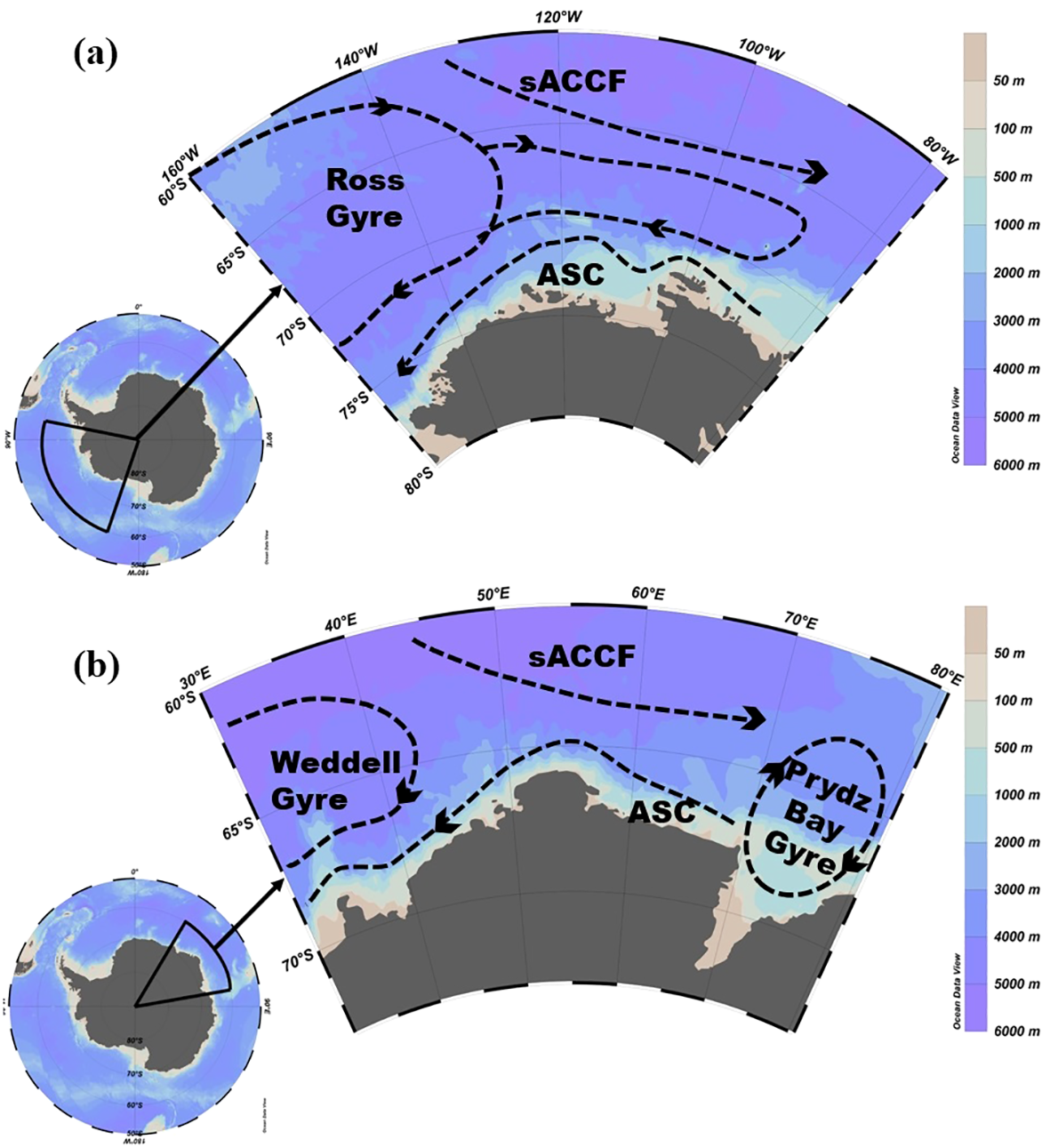
Schematic of the mean circulation in the (a) Amundsen Sea and (b) Cosmonaut Sea. The dashed lines denote the boundaries of each circulation system. (a) In the Amundsen Sea, the primary influences are the Ross Gyre, sACCF, and ASC. (b) In the Cosmonaut Sea, the main influences include the eastern Weddell Gyre, Prydz Bay Gyre, sACCF, and ASC. Ocean circulation patterns are adapted from Williams et al. (2010) and Roach and Speer (2019).
The Cosmonaut Sea, located south of 60°S and between 30°E and 80°E (Figure 1b), also exhibits a complex circulation system. It also includes currents like the sACCF and ASC. South of the sACCF, upwelling processes transport nutrients from subsurface waters to the surface, thereby stimulating phytoplankton growth and significantly influencing the primary productivity of the marine ecosystem (Morrison et al., 2015). Additionally, the Weddell Gyre and the Prydz Bay Gyre play crucial roles in regional ocean dynamics. The Weddell Gyre is characterized by a shallow mixed layer with relatively warm water and low salinity, whereas the Prydz Bay Gyre features a deeper mixed layer with cooler water and higher salinity (Williams et al., 2010).
The Amundsen Sea, situated in the warm-shelf zone, and the Cosmonaut Sea, located in the cold-shelf zone, exhibit differences in CDW temperatures of approximately 1–2°C (Frew et al., 2019; Narayanan et al., 2019). The heat fluxes from the atmosphere and the subsurface water controlled the growth and melting of sea ice (Saenz et al., 2023). In warm-shelf areas, the heat from CDW not only affects the thickness of the ice shelves (Holland et al., 2020) but also influences glacier melt. Conversely, in cold-shelf regions, the thermal effect of CDW is considerably diminished, resulting in increased sea ice production and thicker ice cover (Mahoney et al., 2011).
The study areas in the Amundsen and Cosmonaut Seas were divided into nearshore and offshore regions based on latitude thresholds. Specifically, for the Amundsen Sea, the nearshore region is south of 70°S, and the offshore region was between 60°S and 70°S; for the Cosmonaut Sea, the nearshore region was south of 65°S, and the offshore region was between 60°S and 65°S. This division was based on three reasons: First, these latitude thresholds reflected significant environmental changes identified in January SIC for the Southern Ocean (Supplementary Figure 2). For example, in the Amundsen Sea, areas south of 70°S were near the continental shelf and ice shelves, where sea ice dynamics, while areas north of 70°S were open ocean with less sea ice influence. Second, the division aligned with ocean circulation patterns. In the Amundsen Sea, areas north of 70°S were more influenced by the southern front of the sACCF, while areas south of 70°S were dominated by the ASC, affecting phytoplankton distribution differently; similar patterns apply to the Cosmonaut Sea. Third, although more complex criteria (e.g., distance from the coast, bathymetry, or hydrological fronts) could be used, latitude provided a simple, practical, and repeatable approach that matched the resolution of satellite data and the regional oceanographic context.
2.2 Data collection and match
2.2.1 In situ data
The field survey datasets were obtained from the Chinese Arctic and Antarctic Research Center’s Antarctic expeditions (CHINARE, www.chinare.org.cn) and the Japan National Institute of Polar Research’s Antarctic research team (JARE, www.nipr.ac.jp). The surveys were conducted from 2003 to 2020. A total of 1,896 in-situ Chla data samples and 57 in-situ NPP data samples were collected.
2.2.2 Satellite-derived Chla and NPP
Johnson et al. (2013) performed a comparative analysis of widely used Chla algorithms and found that existing empirical algorithms significantly underestimate Chla in high-latitude regions of the Southern Ocean. As a result, they proposed an improved algorithm for MODIS-OC3M (see Equations 1, 2).
In Equations 1 and 2, R represented the maximum value of the two remote sensing reflectance (Rrs) ratios. Chla_Johnson referred to the Chla data for the Southern Ocean (mg m-3).
The study regions are located in high-latitude regions, where satellite ocean color remote sensing could be influenced by weak illumination due to the low solar zenith angle during winter. Li et al. (2022) used the OC3M algorithm based on MODIS Rrs band ratios and a neural network model to effectively recover hourly Chla products south of 50°S in the Southern Ocean. This Chla product had higher effectiveness and accuracy than the Chla products obtained from MODIS. Therefore, this study adopted the Rrs products from Li et al. (2022) and the improved OC3M algorithm from Johnson et al. (2013). The final Chla_Johnson product spanned from 2003 to 2020, with a spatial resolution of 4 km and a temporal resolution of daily averages (for matching purposes). As a comparison of matching results, this study utilized Level 3 Chla data (Chla_OC3M) obtained from NASA’s MODIS-Aqua (www.oceancolor.gsfc.nasa.gov), covering the period from 2003 to 2020, with a spatial resolution of 4 km and a temporal resolution of monthly averages.
This study used the Vertical Generalized Production Model (VGPM) proposed by Behrenfeld and Falkowski (1997) and the Eppley-VGPM to generate NPP_VGPM and NPP_Eppley products, respectively, based on the Chl_Johnson product as input data. The period for both models was from 2003 to 2020, with a spatial resolution of 1/12° and a temporal resolution of monthly averaged. Additionally, the NPP_Arrigo (mg C m-2 day-1, 4 km and monthly) for the Southern Ocean from 2003 to 2020 was calculated using the NPP algorithm specifically developed for the Southern Ocean by Arrigo et al. (2008), as shown in Equation 3.
where Chla(z) was the Chla at a specific depth z, C/Chla was the ratio of phytoplankton carbon to Chla (constant: 88.5), and G(z, t) was the net biomass-specific growth rate (h−1) at a given time t and depth z.
2.2.3 Matching strategy of in situ data
This study first validated and evaluated satellite-derived Chla against in-situ Chla data. To meet the needs of long-term research, a month was used as the smallest time unit, with an 8-day averaged temporal resolution window to maximize the matching of valid data. Spatially, to minimize the impact of cloud interference and the resulting data gaps, different grid sizes were tested, including 1/6°×1/6°, 1/12°×1/12°, 1/24°×1/24°, and 1/48°×1/48°. The matching process between in-situ and satellite-derived Chla was as follows: First, for each in-situ Chla point, a 3σ criterion was applied for filtering, and satellite datasets within different spatial windows around each in-situ point were identified. Secondly, ensure that there were at least 50% valid pixels in each spatial window, and then used the spatial average method to increase the matching probability and meet the stated accuracy goals for the products (Hu et al., 2001). Thirdly, to ensure homogeneity of the pixel averaging window, data with a coefficient of variation (the ratio of standard deviation to mean) ≥ 0.15 were excluded to ensure stability within each spatial averaging window (Bailey and Werdell, 2006). Finally, the satellite-derived datasets were compared with the corresponding in-situ measurements. A similar matching process was applied to NPP, with a monthly averaged temporal resolution and spatial resolution box of 1/4°×1/4°, 1/6°×1/6°, and 1/24°×1/24°.
2.2.4 Other data
This study utilized environmental parameters such as SST, PAR, WS, MLD, and SIC. SST and PAR data were sourced from NASA’s MODIS-Aqua (www.oceancolor.gsfc.nasa.gov) as level 3 monthly average products, with a spatial resolution of 4 km and a period from 2003 to 2020. Monthly averaged WS datasets, representing wind speed at 10 m above sea level, were obtained from NASA’s QuikSCAT sensor (http://www.remss.com), with a spatial resolution of 0.25° and resampled to a uniform resolution of 4 km. Monthly MLD datasets from 2003 to 2020 were derived using the Hybrid Coordinate Ocean Model (HYCOM), sourced from the Oregon State Ocean Productivity Data Center (www.sites.science.oregonstate.edu), with a spatial resolution of 4 km. SIC data were obtained from the National Snow and Ice Data Center (NSIDC) (https://noaadata.apps.nsidc.org/NOAA) of the National Oceanic and Atmospheric Administration (NOAA), with a spatial resolution of 25×25 km, resampled to a uniform resolution of 4 km. The SIC datasets were available in GeoTIFF format, covering the period from 2003 to 2020 with a monthly temporal resolution. This study incorporated the Southern Annular Mode (SAM) monthly averaged data provided by Marshall (2003).
2.3 Method
2.3.1 Statistical analyses
The following statistical parameters were used to quantitatively assess the validation performance between the in-situ and satellite data:
(1) Pearson correlation coefficient (R), defined as a measure of the linear correlation between the in-situ and satellite data, was calculated in Equation 4:
The statistical significance of each correlation coefficient was assessed using a two-tailed t-test. The p-value was computed from the t-distribution with n–2 degrees of freedom, where n was the sample size. Correlations were considered statistically significant at p < 0.05, corresponding to a 5% significance level.
(2) Root Mean Square Error (RMSE) could be used to evaluate model results, and was calculated in Equation 5:
(3) Bias reflected the systematic deviation of satellite-derived data to in-situ data. The formula referred to Seegers et al. (2018) and was calculated in Equation 6:
(4) Mean Absolute Error (MAE) represented the averaged absolute difference between satellite-derived data to in-situ data, and was calculated in Equation 7:
(5) Median Absolute Percent Difference (MAPD) was the median of all percentage differences, reflecting the typical relative deviation of satellite-derived data from in-situ data, and calculated in Equation 8:
In equations 4 to 8, “RS” and “InSitu” represented the satellite data and in-situ data, respectively; “Predict” and “True” represented the predicted values and true values, respectively; and n was the sample size. In Section 3.1, the MAE and MAPD of the verification process was calculated on a logarithmic scale and then converted back to the original scale.
(6) Spearman Correlation Analysis: to evaluate the relationship between Chla, NPP and environmental variables (SST, PAR, WS, MLD, and SIC), spearman’s rank correlation coefficient was employed. The coefficient was computed in Equation 9:
where denoted the conventional Pearson correlation coefficient operator; cov[r[x], r[y]] was the covariance of the rank variables; σr[x] and σr[y] were the standard deviations of the rank variables. Spearman’s method was robust to skewness and outliers, providing a reliable measure of association under these conditions. The correlation coefficient ρ ranges from -1 to 1, with -1/1 indicating a perfect negative/positive monotonic relationship, and 0 no monotonic relationship. Statistical significance of each correlation coefficient was assessed using a t-test to compute p-values, testing whether ρ significantly differs from zero.
(7) Multiple linear regression. (MLR). This study examined the impact of five environmental factors—SST, PAR, WS, MLD, and SIC—on Chla, not NPP. NPP calculations typically integrate SST, PAR, and MLD, which can introduce autocorrelation or collinearity if analyzed directly with these factors. This study used MLR to quantify their direct relationship with Chla. Focusing on Chla as the dependent variable avoids these issues, allowing a clearer assessment of each factor’s independent contribution. The calculation was as follows:
① Standardization of Data :
In the Equation 10, represented the j-th variable of the i-th sample; had dimensions of , where n was the length of the time series and p was the number of variables (including SST, PAR, WS, MLD, and SIC). was the mean of the j-th variable, and was the standard deviation of the j-th variable. Data standardization was performed to eliminate the influence of different units of measurement.
Before performing MLR analysis, multicollinearity tests were performed on environmental factors (x) to assess potential multicollinearity problems (see Supplementary Table 2).
② Assuming a linear relationship between the dependent variable and independent variables, the linear equation was as follows:
In the Equation 11, were the regression coefficients of each independent variable, indicating the extent of the impact of each independent variable on the dependent variable; ε epsilonϵ was the error term, representing the unexplained portion of the model. After standardization, the relative contribution of each independent variable could be assessed by comparing the absolute values of the regression coefficients.
③ The percentage contribution of each parameter was calculated in Equation 12:
where βi was the coefficient for the i-th environmental parameter, and the summation includes all predictors in the model.
2.3.2 Calculation of long-term series change trend
To quantify the long-term trends of Chla and NPP in the study areas, the Mann-Kendall (MK) test (Mann, 1945; Kendall, 1975) combined with the Sen slope (Sen, 1968) were applied for robust climate change analysis (Thomalla et al., 2023; Pinkerton et al., 2021). Based on MATLAB software to achieve, the specific steps are as follows (Chla as an example):
First, climatological monthly averages were calculated for each month (e.g., January, February, etc.) using the entire time series of satellite-derived Chla. These averages were subtracted from the corresponding monthly values to derive anomaly data, effectively removing the influence of seasonal fluctuations. For each pixel within the target regions, MK test was defined in Equation 13:
where xi and xj were data points in the time series, and sgn was the sign function (1 if xj−xi> 0, -1 if < 0, and 0 if = 0). The sign of MK indicated an upward or downward trend, with statistical significance determined by the standardized statistic Z and corresponding p-value.
Upon confirming trend significance, this study quantified the trend magnitude using Sen slope estimator, calculated as the median of all pairwise slopes. See Equation 14.
where Sen represented the rate of change per unit time. This non-parametric method was also robust against outliers. For pixels where the p-value exceeded 0.05 (p > 0.05), the trend was deemed non-significant, and the Sen slope was set to 0 to exclude these statistically unreliable trends from further analysis. This thresholding ensured that only robust trends contributed to the regional assessment.
3 Result
3.1 Validation of satellite-derived Chla and NPP
To evaluate the reliability of satellite-derived data products for assessing phytoplankton productivity, we compared satellite-derived Chla and NPP estimates with corresponding in-situ measurements. The validation was performed across multiple spatial resolutions using two Chla products: Chla_OC3M and Chla_Johnson, and three NPP models: NPP_VGPM, NPP_Eppley, and NPP_ Arrigo.
The results of the in-situ and satellite-derived Chla match-ups were shown in Figure 2, and the spatial distribution results were shown in Supplementary Figure 1. Typically, when the two datasets lie near the 1:1 line, it indicates high matching accuracy. If the satellite data lie above the 1:1 line, they overestimate the in-situ data, and vice versa. Figures 2a–c showed that the Chla_OC3M generally underestimated the in-situ Chla data. In contrast, the Chla_Johnson product (Figures 2e–h), derived using the modified OC3M algorithm, exhibited improved agreement with in-situ measurements and aligned more closely with the 1:1 line. This improvement was reflected in a lower MPD, meeting the NASA Ocean Color Protocol requirement of ±35% accuracy (Hooker and McClain, 2000). The other statistical results of each spatial window confirmed that Chla_Johnson (Figures 2e–h) was also more effective and accurate than Chla_OC3M (Figures 2a–d). NPP validation results were shown in Figure 3. Both the VGPM and Eppley models (Figures 3a–f) tended to underestimate in-situ NPP values across spatial scales. Although NPP_Arrigo showed a slight overestimation, considering that the MAPD and MAE of NPP_Arrigo (1/4° and 1/6°) were the smallest and the bias was closer to 1, indicated that this product had better stability (Figures 3g, h). However, the performance metric of the 1/12° box of NPP_Arrigo indicated that the high-resolution window was not suitable for high latitude sea areas. This might result from fewer matching points due to reduced average effective pixels at higher window resolutions and the removal of highly variable pixels through strict quality screening. In addition, the simulation of the algorithm for sub-mesoscale features needs to be strengthened to further reduce the deviation between the predicted and observed values.
Figure 2
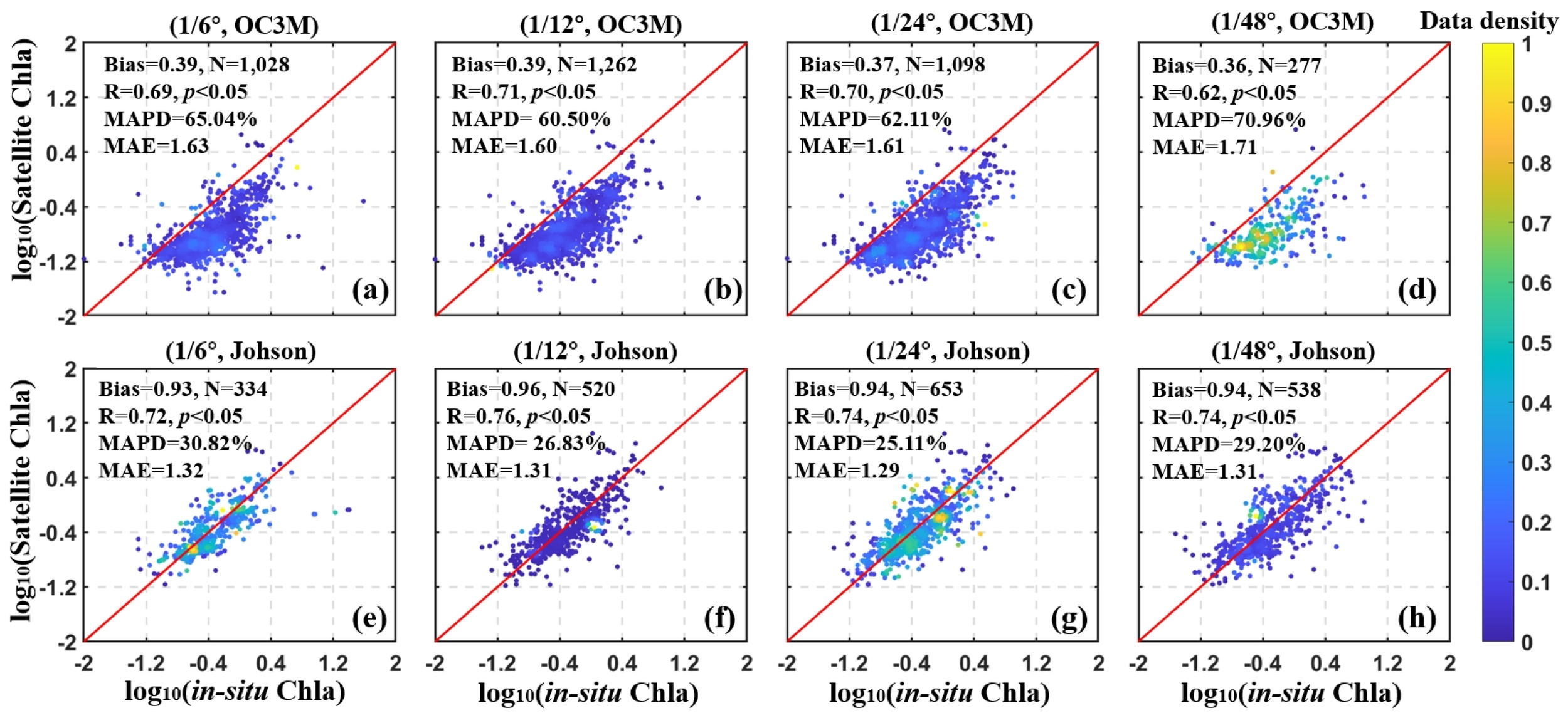
Validation results of satellite-derived Chla and in-situ Chla (Unit: mg m-3) with spatial resolution of 1/6° (a, e), 1/12° (b, f), 1/24° (c, g) and 1/48° (d, h). (a–d) Match-ups from Chl_OC3M and in-situ Chla; (e–h) Match-ups from Chl_Johnson and in-situ Chla. The units of Bias and MAE were mg m-3.
Figure 3
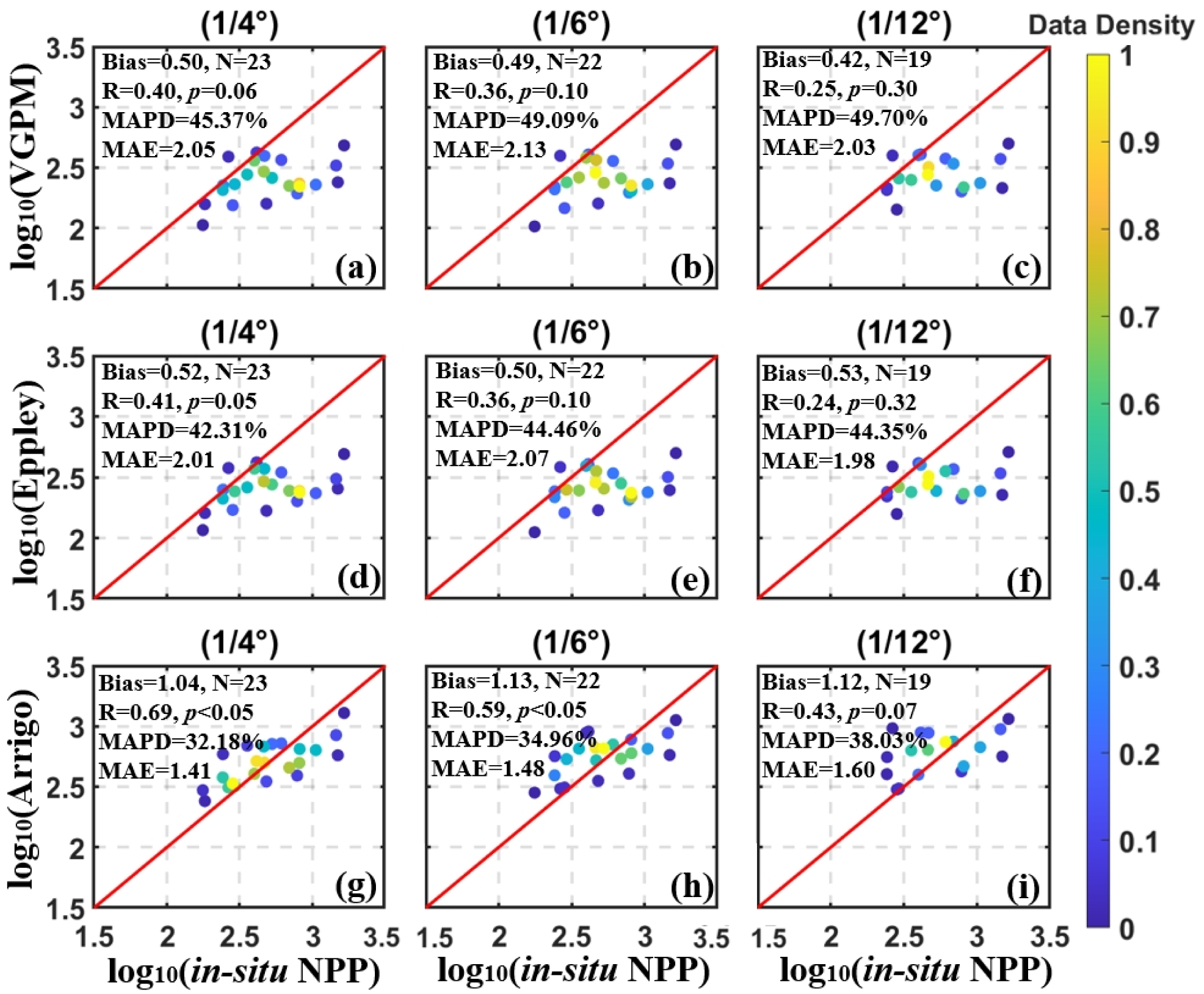
Validation results of satellite-derived NPP and in-situ NPP (Unit: mg C m-2 day-1) with spatial resolution of 1/4° (a, d, g), 1/6° (b, e, h) and 1/12° (c, f, i). (a–c) Match-ups from NPP_VGPM and in-situ NPP; (d–f) Match-ups from NPP_Eppley and in-situ NPP; (g–i) Match-ups of NPP_Arrigo and in-situ NPP. The units of Bias and MAE were mg C m-2 day-1.
Overall, the accuracy verification quantitatively showed that the match-ups of Chla_Johnson and NPP_Arrigo were consistent with in-situ observations and exhibited significant correlations. These validated datasets were therefore adopted in the subsequent analyses of spatiotemporal variability and trend detection in the Amundsen and Cosmonaut Seas.
3.2 Spatial and temporal variability of Chla and NPP in the Amundsen and Cosmonaut Seas
Satellite-derived Chla and NPP data from 2003 to 2020 revealed distinct seasonal and spatial patterns across the Amundsen and Cosmonaut Seas (Figure 4). Both variables exhibited strong variability, with phytoplankton biomass and productivity typically increasing from November, peaking in January, and declining through February and March.
Figure 4
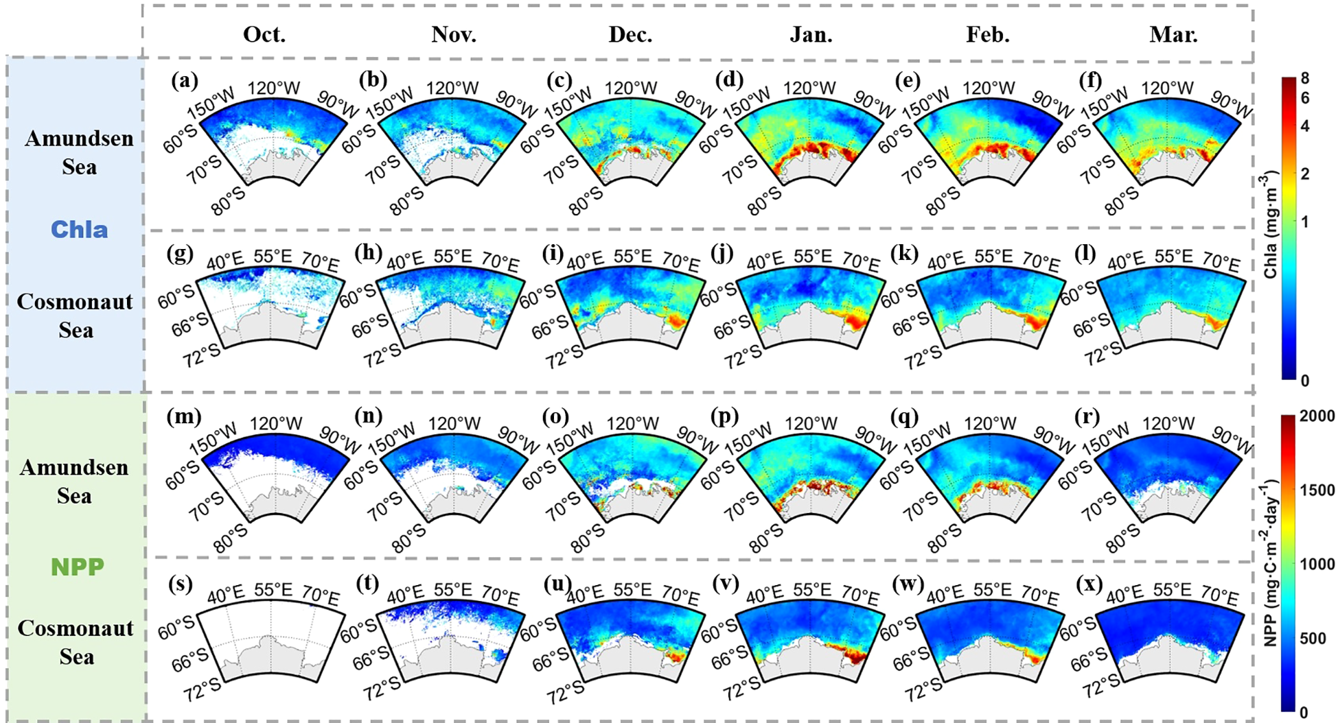
Climatological monthly mean of Chla (a–l), NPP (m–x) in the Amundsen and Cosmonaut Seas from 2003 to 2020.
Spatially, higher spatial mean Chla and NPP values were consistently observed in nearshore regions compared to offshore areas. In the Amundsen Sea, summertime (December–February) mean values of Chla and NPP reached 1.18 mg m-3 and 824.44 mg C m-2 day-1, respectively, while the corresponding values in the Cosmonaut Sea were 0.64 mg m-3 and 611.83 mg C m-2 day-1. Within the nearshore zone, maximum values were observed south of 70°S in the Amundsen Sea (up to 1.63 mg m-3 Chla and 903.82 mg C m-2 day-1 NPP) and south of 65°S in the Cosmonaut Sea (up to 0.87 mg m-3 Chla and 637.41 mg C m-2 day-1 NPP). This nearshore–offshore gradient was most pronounced in January, when the difference between the two zones peaked (Amundsen Sea: ΔChla = 1.00 mg m-3, ΔNPP = 417.65 mg C m-2 day-1; Cosmonaut Sea: ΔChla = 0.38 mg m-3, ΔNPP = 226.79 mg C m-2 day-1).
Within the offshore domains, the western Amundsen Sea, corresponding to the Ross Gyre divergence zone, exhibited elevated productivity compared to its eastern counterpart. In the Cosmonaut Sea, localized high-productivity areas were observed in the Prydz Bay and the eastern part of the Weddell Gyre, with peak values reaching 1.39 mg m-3 for Chla and 874.03 mg C m-2 day-1 for NPP in the Prydz Bay.
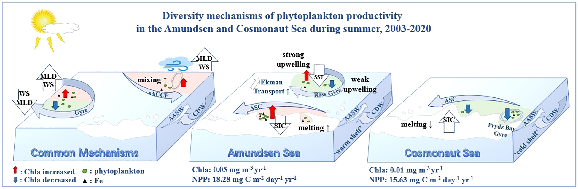
Long-term trends in austral summer Chla and NPP were assessed using Sen slope and MK test (Figure 5). Seasonal variations in Chla and NPP in the Amundsen and Cosmonaut Seas as a whole, offshore, and nearshore regions were summarized in Table 1. Both seas exhibited significant positive trends in their spatially averaged productivity over the 18-year period. In the Amundsen Sea, Chla increased at a rate of 0.05 mg m-3 yr-1 and NPP at 18.28 mg C m-2 day-1 yr-1. Corresponding trends in the Cosmonaut Sea were slightly lower: 0.01 mg m-3 yr-1 for Chla and 15.63 mg C m-2 day-1 yr-1 for NPP.
Figure 5
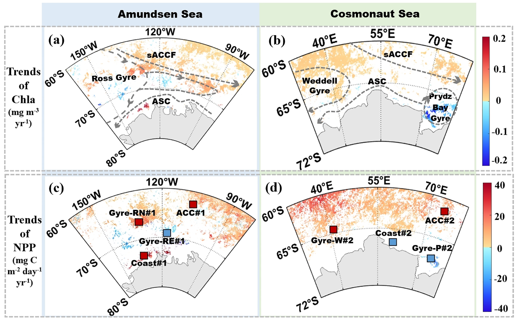
Averaged trends of Chla (a, b) and NPP (c, d) in the Amundsen (a, c) and Cosmonaut Sea (b, d) in austral summer (December to February) from 2003 to 2020. Only statistically significant trends were shown (p < 0.05).
Table 1
| Summer\Seas | Amundsen Sea | Cosmonaut Sea | |
|---|---|---|---|
| Chla | Whole Sea | 0.05 | 0.01 |
| Offshore | 0.04 | 0.08 | |
| Nearshore | 0.12 | -0.13 | |
| NPP | Whole Sea | 18.28 | 15.63 |
| Offshore | 14.20 | 18.11 | |
| Nearshore | 20.09 | -8.57 | |
Spatially averaged rates of change for Chla and NPP in austral summer in the target regions.
The rate of Chla (unit: mg m-3 yr-1) was followed by the rate of NPP (unit: mg C m-2 day-1 yr-1). Excluding non-significant trends (p > 0.05), only significant trends were shown.
At the subregional level, the offshore areas in the Amundsen Sea exhibited spatial mean Chla and NPP increases of 0.04 mg m-3 yr-1 and 14.20 mg C m-2 day-1 yr-1, respectively. In the nearshore region of the Amundsen Sea, both Chla and NPP are higher than offshore areas (Figure 5, Table 1). Notably, increases were observed north of the sACCF and in the northern Ross Gyre, while decreases were noted in the southern and eastern parts of the Ross Gyre. The offshore areas in the Cosmonaut Sea showed increased trends, with 0.08 mg m-3 yr-1 in Chla and 18.11 mg C m-2 day-1 yr-1 in NPP. In contrast, the nearshore Cosmonaut Sea, particularly the region encompassing the Prydz Bay, which displayed negative trends, with Chla and NPP decreasing by -0.13 mg m-3 yr-1 and -8.57 mg C m-2 day-1 yr-1, respectively.
3.3 Environmental parameter variability and correlation patterns in the Amundsen and Cosmonaut Seas
The environmental parameters considered in this study built on previous research on the impacts of climate change on primary producers in the Southern Ocean (Pinkerton et al., 2021). Key environmental drivers, including SST, PAR, WS, MLD, and SIC, were incorporated to enhance understanding of the primary factors and regulatory mechanisms influencing phytoplankton biomass and productivity in the Amundsen and Cosmonaut Seas.
Figure 6 presented the monthly variations of these parameters in the Amundsen and Cosmonaut Seas during the austral summer (November to March) from 2003 to 2020. SST and PAR in the Amundsen and Cosmonaut Seas initially increased in November, with SST peaking in February and PAR peaking in December, followed by a decline (Figures 6a, b, f, g). Conversely, WS and MLD exhibited an inverse trend, reaching their lowest values in December and January (regional averages: Amundsen Sea: 5.52 m s-1 and 22.11 m; Cosmonaut Sea: 5.73 m s-1 and 20.62 m; Figures 6c, d, h, i). SIC data revealed that both regions were predominantly ice-free from December to March (Figures 6e, j). During the austral summer period (December and January), the marine environment demonstrated greater stability, characterized by ice-free conditions, warmer SST, higher PAR, and reduced wind speeds (Figure 6). These conditions were more conducive to large-scale phytoplankton blooms compared to other months (Figure 4).
Figure 6
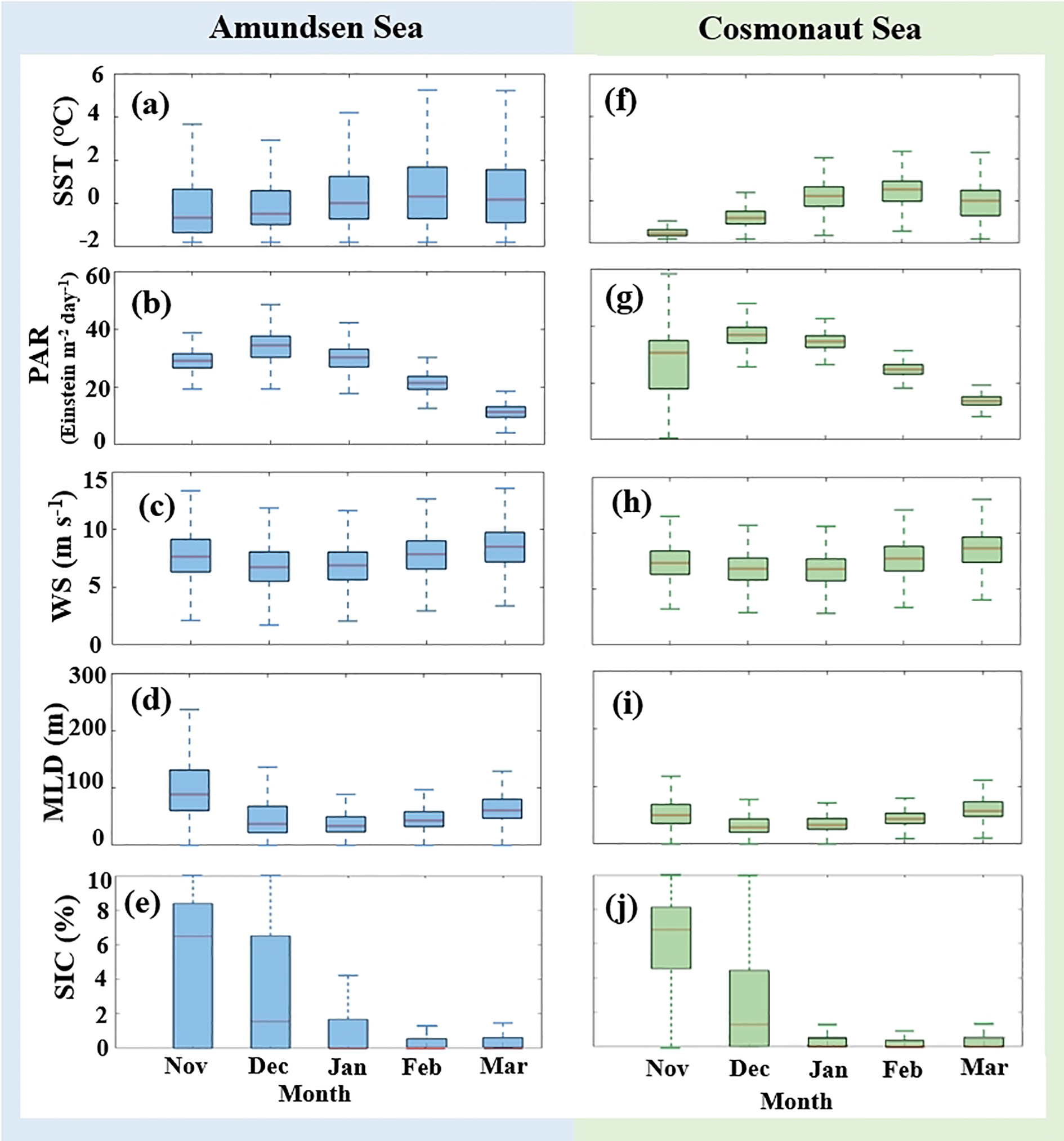
(a–j) Box plots of various environmental parameters (SST, PAR, WS, MLD, and SIC) in the Amundsen and Cosmonaut Seas from November to March, 2003–2020. The red lines showed the median.
To further investigate the primary environmental drivers of marine phytoplankton productivity, the long-term trends of various parameters during the austral summer (2003–2020) were analyzed (Figure 7, Supplementary Figure 3). In the offshore regions, long-term results showed increasing trends in WS, MLD, and SIC, while SST and PAR decreased significantly (p < 0.05, n = 54, Supplementary Figure 3). Long-term observations indicated that SIC differed significantly between nearshore and offshore regions of the Amundsen Sea. Similarly, WS exhibited distinct spatial variability between nearshore and offshore regions of the Cosmonaut Sea (p < 0.05, n = 54, Supplementary Figure 3).
Figure 7
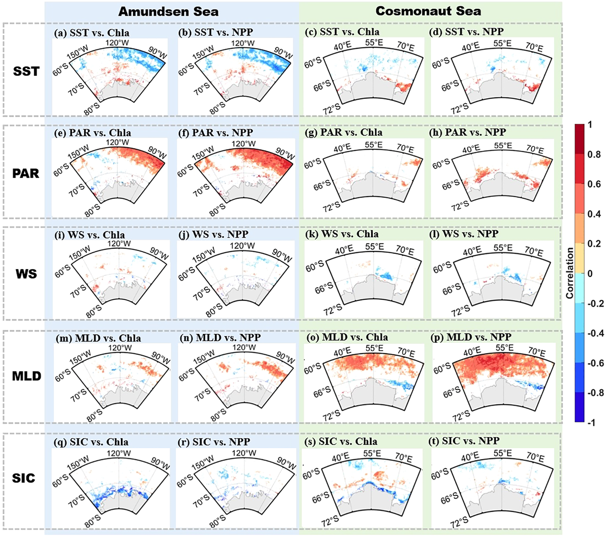
(a–t) Spearman correlations of SST, PAR, WS, MLD, and SIC in the Amundsen (a–h) and Cosmonaut (i–p) Seas with Chla and NPP, respectively, during austral summer 2003–2020 (p < 0.05). Note: before correlation analysis, the data were detrended.
To quantify the relationships between environmental variability and phytoplankton responses, Spearman correlation analyses were conducted between detrended environmental time series and Chla/NPP in both offshore and nearshore regions (Figure 7). In the offshore areas, correlation results indicated that when SST was the independent variable, Chla and NPP increased as SST decreased (Figures 7a–d, p < 0.05, n = 54). Conversely, when PAR, MLD, and SIC were the independent variable, respectively, Chlan and NPP showed a positive correlation with these parameters (Figures 7e–h, m–t, p < 0.05, n = 54). In the nearshore areas, phytoplankton productivity was significantly positively correlated with SST, PAR, and MLD (Figures 7a–h, m–p, p < 0.05, n = 54), while it was negatively correlated with SIC (Figures 7q–t, p < 0.05, n = 54).
These spatially varying correlation patterns indicate differing sensitivities of phytoplankton productivity to environmental drivers depending on geographic setting. Offshore productivity appeared to be more closely associated with vertical mixing and stratification processes, while nearshore variability was more strongly linked to thermal and radiative conditions and sea ice coverage. These observations provide a quantitative foundation for the region-specific mechanistic analyses that follow in the Discussion section.
3.4 Environmental parameter contributions to Chla variability in the Amundsen and Cosmonaut Seas
To quantify the influence of environmental variables on Chla variability, eight 1°×1° subregions in the Amundsen and Cosmonaut Seas were selected based on circulation patterns and significant Chla trends (Figures 5a, b), adopting a 1°×1° box scale inspired by S. Zhang et al. (2023) to capture mesoscale oceanographic features like sea ice dynamics regions and frontal zones using satellite-derived Chla and NPP data (4 km resolution, 2003–2020), thereby reducing noise while preserving regional signals. These include two subregions near the sACCF in the Amundsen and Cosmonaut Seas (ACC#1 and ACC#2), two nearshore zones influenced by coastal currents (Coast#1 and Coast#2), two areas in the Ross Gyre (Gyre-RN#1 and Gyre-RE#1), and two in the Cosmonaut Sea associated with the Weddell Gyre and Prydz Bay Gyre (Gyre-W#2 and Gyre-P#2).These eight sub-regions were used to analyze the differences in the mechanisms by which changes in environmental parameters affect phytoplankton in the sACCF, Gyre, and nearshore areas of the Amundsen Sea and Cosmonaut Sea.
In the subregions north of the sACCF, ACC#1 (averaged: 0.43 mg m-3, 655.68 mg C m-2 day-1) and ACC#2 (averaged: 0.60 mg m−3, 637.02 mg C m-2 day-1) exhibited relatively lower phytoplankton productivity compared to other subregions. However, both subregions demonstrated increasing trends over the study period (p < 0.05, n = 54, Figure 4, Supplementary Table 1). Based on multiple linear regression indicated that strengthened WS and MLD were the primary contributors to observed increased Chla (Table 2). Specifically, WS and MLD accounted for 40.56% and 18.17% of Chla variance in ACC#1, while MLD alone explained 64.82% in ACC#2. Both regions exhibited positive correlations between MLD and Chla, indicating that Chla increased as MLD deepened (p < 0.05, Figure 7, Figures 8a–d).
Table 2
| Regions/Parameters | SST | PAR | WS | MLD | SIC | RMSE | |
|---|---|---|---|---|---|---|---|
| Amundsen | ACC#1 | 0.02 | 0.02 | -0.09 | 0.06 | 0.08 | 0.25 |
| 1.18% | 2.84% | 40.56% | 18.17% | 37.24% | |||
| Gyre-RN#1 | -0.08 | -0.01 | -0.07 | 0.03 | 0.01 | 0.44 | |
| 54.82% | 1.00% | 34.20% | 9.20% | 0.78% | |||
| Gyre-RE#1 | 0.18 | 0.02 | -0.11 | 0.11 | 0.01 | 0.37 | |
| 56.90% | 0.94% | 22.53% | 19.52% | 0.11% | |||
| Coast#1 | 1.29 | -0.23 | 0.37 | 0.28 | -0.94 | 1.96 | |
| 58.89% | 1.96% | 4.91% | 2.74% | 31.50% | |||
| Cosmonaut | ACC#2 | 0.08 | 0.17 | -0.04 | 0.26 | 0.03 | 0.31 |
| 5.83% | 26.86% | 1.59% | 64.82% | 0.90% | |||
| Gyre-W#2 | 0.11 | 0.14 | -0.04 | 0.16 | -0.12 | 0.45 | |
| 10.77% | 18.06% | 1.15% | 57.29% | 12.73% | |||
| Gyre-P#2 | 0.37 | 0.01 | -0.12 | -0.30 | 0.06 | 1.37 | |
| 55.96 | 0.01% | 5.56% | 37.16% | 1.31% | |||
| Coast#2 | 0.07 | -0.06 | -0.15 | 0.05 | -0.35 | 0.22 | |
| 3.18% | 2.26% | 15.48% | 1.90% | 77.18% | |||
Multiple regression coefficients and the contribution of each marine environmental parameter (SST, PAR, WS, MLD, and SIC) to Chla of 8 subregions in the Amundsen and Cosmonaut Seas, respectively.
For each environment parameter in the table, the first row was the regression coefficient, and the second row was the contribution percentage. Unit of RMSE was mg m-3.
Figure 8
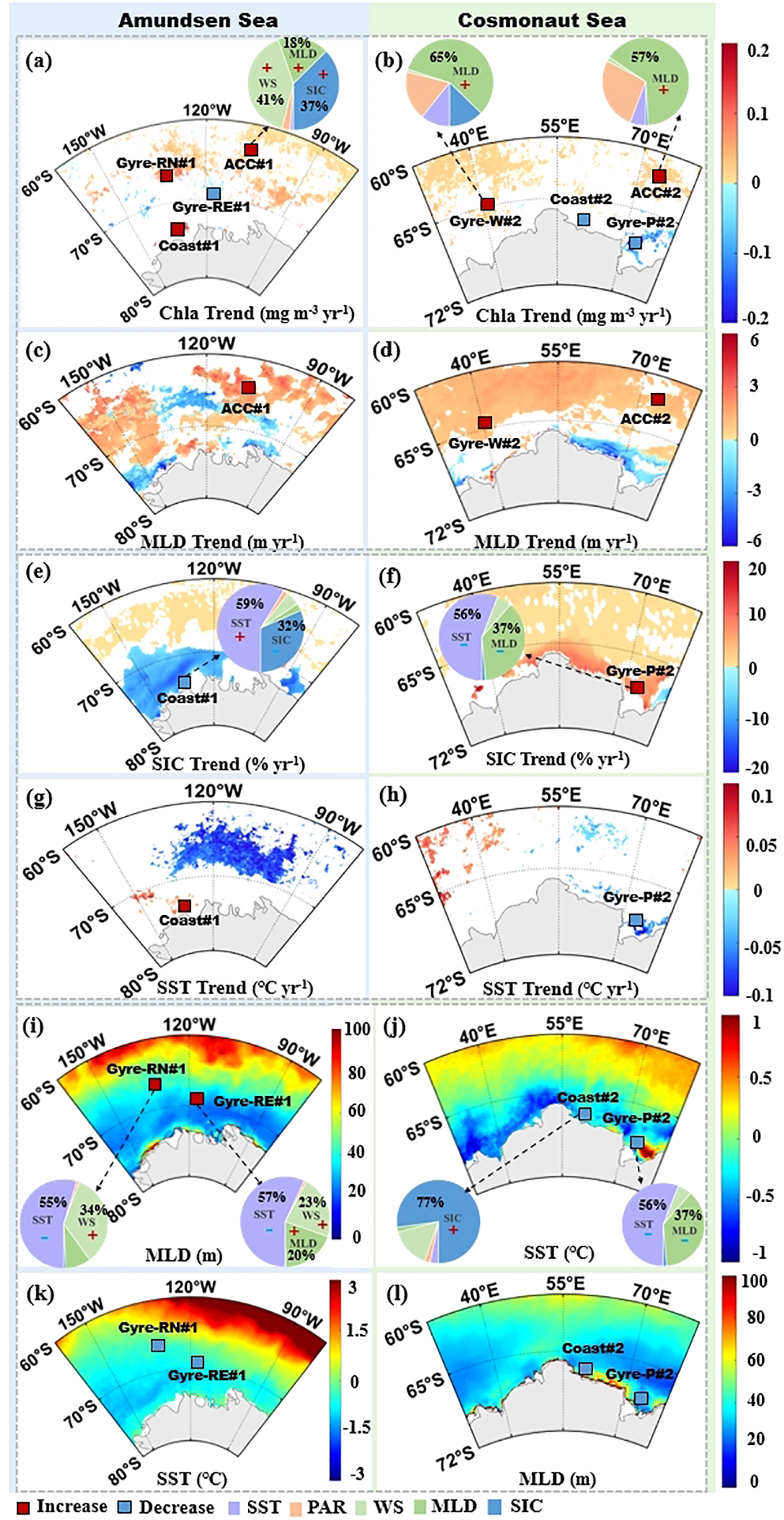
(a–l) Contribution ratio diagram of environmental parameters (SST, PAR, WS, MLD, and SIC) to Chla variation in the Amundsen and Cosmonaut Sea during austral summertime, 2003 to 2020. Note: the plus or minus signs indicated an increase or decrease in trend, and the values of all contributions were rounded to integers.
Environmental trends in Gyre-W#2 was comparable to those observed in ACC#1 and ACC#2 (Supplementary Figure 4), characterized by increasing Chla and NPP (Supplementary Table 1). The contribution of MLD deepening to Chla was most significant (57.29%, Figure 8b, Table 2). A notable positive correlation was found between WS and MLD (Supplementary Figure 4, Table 2, R = 0.59, p < 0.05), which implied that the mechanism controlling the increase in Chla was likely to be consistent in Gyre-W#2 and ACC#1 as well as ACC#2.
In Coast#1, the nearshore Amundsen Sea region, situated in highly productive nearshore regions, characterized by averaged Chla and NPP values of 2.77 mg m−3 and 1,498.16 mg C m−2 day−1, respectively. Warming SST showed a significant positive correlation with both Chla and NPP, while SIC was negatively correlated (p < 0.05, Figure 7). Both Chla and NPP demonstrated significant increasing trends over the study period (p < 0.05, n = 54, Supplementary Table 1). SST and SIC accounted for approximately 58.89% and 31.50% of the increased Chla, respectively (Figure 8e, Table 2). Furthermore, SST and SIC were significantly negatively correlated, indicating a robust relationship between SIC melting and SST warming (p < 0.05, n = 54, Supplementary Figure 4). Additionally, increased WS and deepened MLD contributed less to Chla variability (Figures 8e, g, Table 2).
This study also identified that the Prydz Bay Gyre exhibited significant large-scale algal blooms (Figure 4). However, during the austral summer of 2003–2020, these blooms in Gyre-P#2 exhibited a significant declining trend (-0.10 mg m-3 yr-1, p < 0.05, Figure 5), consistent with the findings of Pinkerton et al. (2021), who observed a decreasing trend in Chla in the Prydz Bay. Cooling SST accounted for approximately 55.96% of the Chla decline (Figures 8f, h, Table 2, Supplementary Figure 3, 4). Concurrently, decreased MLD exhibited a significant negative correlation with Chla (p < 0.05, Figure 7). Although MLD contributed 37.16%, this indirectly reflected that the reduction of Chla was not caused by MLD, but by SST. A similar situation was observed in Coast#2 (Table 8j). Both Chla (-0.01 mg m-3 yr-1) and NPP (-1.95 mg C m-2 day-1 yr-1) exhibited declining trends (p < 0.05, n = 54). Notably, the increased SIC (0.80% yr-1, Supplementary Figure 3) explained approximately 77.18% of decreased Chla, and SIC and Chla were significantly negatively correlated (R = -0.57, p < 0.05). For every unit increase in SIC, Chla decreased by -0.35 mg m-3 (Table 2).
The two Ross Gyre subregions (Gyre-RN#1 and Gyre-RE#1) exhibited similar response patterns in terms of contributing variables (Figures 8i, k, Supplementary Figure 4). In Gyre-RN#1, cooling SST and strengthened WS accounted for 54.82% and 34.20% of Chla variability, respectively (Supplementary Figure 3, Figure 8i). In Gyre-RE#1, SST and WS contributions were 56.90% and 22.53%, respectively (Supplementary Figure 3, Figure 8i). Despite both regions being part of the same circulation system, only Gyre-RN#1 showed a positive trend in Chla, whereas Gyre-RE#1 displayed a decline. This indicated that the mechanisms driving productivity changes in Gyre-RE#1 differ markedly from those observed in Gyre-RN#1.
4 Discussion
4.1 Climate regulation of phytoplankton dynamics in the Amundsen and Cosmonaut Seas
Long-term variability in phytoplankton productivity in the Amundsen and Cosmonaut Seas is not only shaped by local environmental factors but also modulated by large-scale atmospheric and oceanic climate drivers (Lenton and Matear, 2007). Among these, the Southern Annular Mode (SAM) emerges as a key mechanism linking atmospheric variability with upper-ocean conditions (Thompson et al., 2011). As the dominant mode of climate variability in the Southern Hemisphere, the SAM controls the intensity and latitudinal position of the westerly wind belt (Marshall, 2003; Fogt and Marshall, 2020). In recent decades, the SAM has exhibited a persistent trend toward its positive phase, characterized by stronger and poleward-shifted westerlies (Thompson et al., 2011; Perren et al., 2020). This shift enhances Ekman-driven upwelling and promotes the equatorward transport of cold surface waters, leading to SST cooling in much of the Southern Ocean (Purich et al., 2016; Xu et al., 2022). Furthermore, SAM exerts significant influence on changes in MLD and mesoscale eddies (Screen et al., 2010; Sen Gupta and England, 2006), ultimately influencing nutrient transport and variations in phytoplankton concentration (Noh et al., 2021).
According to the cross-correlation analysis of SAM with Chla and NPP, the change of SAM positively affected the change on Chla and NPP (Supplementary Figure 5). The increasingly positive phase of SAM enhances near polar cold water mixing through changes in wind speed (Fogt and Marshall, 2020; Marshall, 2003; Thompson et al., 2011). Consequently, this process modifies the thickness and depth of the Southern Ocean’s mixed layer (Screen et al., 2010), redistributes nutrients, and ultimately influences marine ecosystem productivity (Noh et al., 2021).
In the Amundsen Sea, positive SAM conditions facilitate the southward intrusion of warm CDW onto the continental shelf (Deb et al., 2018; Naughten et al., 2023). In contrast, regions such as the Cosmonaut Sea appear less responsive to SAM induced upwelling due to persistent sea ice cover and more limited access to CDW intrusions, resulting in decreased productivity trends. These climate influences interact with local dynamics to create complex patterns of phytoplankton variability. While SAM intensification generally promotes vertical nutrient transport through stronger winds and deeper MLD, the regional biological response depends on concurrent SIC conditions, SST anomalies, and iron availability, emphasizing the need for regionally interpretation of climate signals.
4.2 Mechanistic explanations of phytoplankton variation in the Amundsen and Cosmonaut Seas
The spatial heterogeneity in phytoplankton trends across the Amundsen and Cosmonaut Seas reflects the influence of distinct environment and region-specific physical forcing. Differences between nearshore and offshore zones, as well as between gyre and frontal areas, suggest that phytoplankton productivity in this region of the Southern Ocean is regulated by the combined effects of SST, SIC, MLD, and so forth. These environmental factors could be synergistic or antagonistic, and determining the net effect of these interactions on phytoplankton biomass and productivity remains challenging (Thomalla et al., 2023).
In most regions of the Amundsen and Cosmonaut Seas, MLD and WS showed a significant positive correlation, indicating that the deepening of MLD was mainly driven by the enhancement of WS. Carranza and Gille (2015) argued that if the intensity of wind-driven mixing is sufficient to deepen MLD, MLD may play a key role in the increase of phytoplankton in summer. For the subsequent sub-regions, if the change in MLD is caused by WS, which is referred to as wind-driven MLD here.
In high-nutrient, low-chlorophyll (HNLC) systems such as the Southern Ocean, vertical nutrient transport is crucial for sustaining phytoplankton productivity (Carranza and Gille, 2015). Wind-driven MLD deepening facilitates the upward flux of macronutrients and micronutrients, especially iron into surface waters (Carranza and Gille, 2015; Fauchereau et al., 2011). Under adequate light conditions, this process supports phytoplankton growth. However, the effect of MLD on productivity depends on local iron limitation: when iron limitation is strong, MLD deepening generally promotes growth, but when iron is already sufficient, excessive mixing may dilute surface concentrations or reduce light exposure, resulting in a negative correlation between MLD and Chla (Fauchereau et al., 2011).
Vertical mixing, however, is not the only pathway for iron supply in the Southern Ocean. In nearshore regions adjacent to the Antarctic continent, sea-ice and glacial meltwater release iron-rich freshwater into the upper ocean. This freshwater input enhances water column stratification while simultaneously delivering iron, thereby stimulating phytoplankton growth through a mechanism that operates independently of deep vertical mixing (Behera et al., 2020; Leung et al., 2015; Petrou et al., 2016). As a result, the increase in the nearshore Chla may require further consideration of the effects brought about by the SST and SIC relationship.
Three primary mechanisms governing Chla and NPP dynamics had been identified in the Amundsen and Cosmonaut Seas (Figure 9). The first mechanism involved wind-driven changes in MLD, which significantly influenced phytoplankton dynamics. In the regions north of the sACCF in the Amundsen and Cosmonaut Seas, as well as the Weddell Gyre, the observed increase in phytoplankton biomass and productivity during austral summers from 2003 to 2020 was predominantly attributed to wind-driven MLD enhancement. WS exhibited a significant positive correlation with MLD (Supplementary Figure 4), suggesting that WS enhanced vertical mixing in the upper ocean, thereby deepening the MLD (Carranza and Gille, 2015). This process facilitated the upwelling of nutrient-rich subsurface waters to the surface (Sallée et al., 2021), contributing to the sustained long-term increase in regional phytoplankton productivity (Figure 9).
Figure 9
Schematic diagram of the austral summer Chla and NPP trends mechanisms.
Moderate wind speed anomalies can break the surface stratification, enhance vertical mixing (deepen the MLD), thereby transporting deep nutrients to the surface and supporting the increase of Chla (Fauchereau et al., 2011; Carranza and Gille, 2015). However, overly strong wind speeds may deepen the MLD below the euphotic layer and inhibit the growth of phytoplankton (Fitch and Moore, 2007). In ACC#1, WS contributed high but showed a negative effect, which was consistent with the negative correlation between WS and Chla in the Southern Ocean at the monthly and seasonal scales (Fitch and Moore, 2007). While, in ACC#2, the contribution of WS was relatively low, and its indirect impact through the deepening of MLD was limited. The negative regression coefficient indicated that strong winds were not conducive to the increase of Chla (Table 2). Regression analysis effectively distinguished the direct negative effect of WS on Chla (due to excessive mixing) and the indirect positive effect (due to moderate deepening of MLD).
The impact of the ACC#1 area on SIC in offshore cannot be ignored, the contribution of cooling SIC was significant. It was inferred that cooling SST led to an increase in SIC, reducing stratification and enhancing vertical mixing, which combined with wind-driven mixed layer deepening, promoted phytoplankton growth in the region.
Concerning the impact on the Weddell Gyre, the findings of Williams et al. (2010) on large-scale circulation in the Cosmonaut Sea indicate that the eastern boundary of the Weddell Gyre demonstrated relatively high levels of productivity, with Gyre-W#2 being identified as an upwelling region (Westwood et al., 2010). Although PAR also contributed to the increase in Chla, highlighting its role in enhancing phytoplankton productivity under unrestricted light conditions, wind-driven enhancement of MLD in Gyre-W#2 remained the main driver of phytoplankton outbreaks.
The second mechanism involved the influence of upwelling intensity on phytoplankton responses. During the positive phase of SAM, intensified westerly winds induce Ekman transport, which moves cooler SST from south to north (Xu et al., 2022). This process enhanced upwelling and resulted in decreased SST in both subregions of the Ross Gyre. In Gyre-RN#1, the cooling of SST, combined with wind-driven MLD, brought nutrient-rich cold water from deeper layers to the surface, thereby promoting phytoplankton blooms in this region (Figure 8e). In contrast, Gyre-RE#1, situated between sACCF and Southern Boundary Front, exhibited higher averaged Chla and NPP than ACC#1. These observations were consistent with previous studies indicating that productivity is often elevated near frontal zones (Boyd et al., 1995). However, the average austral summer MLD in Gyre-RE#1 was significantly shallower than in Gyre-RN#1. Furthermore, the SST cooling rate in Gyre-RE#1 was considerably lower than in Gyre-RN#1, which might suggest weaker upwelling activity in Gyre-RE#1. With a shallower MLD, nutrient availability from subsurface waters might also be reduced. Strass et al. (2002) demonstrated that alternating upwelling and downwelling motions frequently occur near polar fronts. Due to the fast surface currents of the ACC, downwelling areas are usually associated with increased Chla, downwelling areas are typically characterized by higher Chla concentrations, while upwelling regions, despite their nutrient richness, may exhibit lower Chla levels (Hense et al., 2003). These factors likely contributed to the observed decline in phytoplankton productivity in subregion Gyre-RE#1 (Figure 9).
A third mechanism influencing phytoplankton variability involves the coupling between SST and SIC, particularly in coastal regions where basal melting and meltwater dynamics strongly modulate ecological conditions. In nearshore Amundsen region, elevated SST is associated with reduced SIC, leading to prolonged open-water periods, enhanced light penetration, and stratified conditions favorable to bloom development (Petrou et al., 2016; Sherrell et al., 2015). Although wind speed had a relatively minor direct contribution to productivity in this region, synoptic-scale winds can influence the size and persistence of polynyas by regulating sea ice extent (Arrigo et al., 2012). Downslope wind events may also enhance vertical mixing along the coastal slope, promoting nutrient resupply in the marginal ice zone (DeJong et al., 2018). Overall, the observed increase in phytoplankton productivity in the nearshore region of the Amundsen Sea resulted from a synergistic effect where warming SST promoted SIC melting, and wind-driven MLD deepening enhanced nutrient availability (Figure 9).
In contrast, the nearshore Cosmonaut Sea represents a colder shelf system characterized by persistent sea-ice cover and limited thermal forcing (Narayanan et al., 2019). Observed declines in SST and increases in SIC (both significantly negatively correlated, p < 0.05, n = 54) in nearshore Cosmonaut regions likely reduce the delivery of meltwater-derived nutrients (Fe), contributing to the long-term decline in phytoplankton productivity (Figure 9). DeJong et al. (2018) indicated that strong coastal winds during the austral summer inhibit coastal ice melt, and wind-induced sea ice retreat remains minimal farther offshore. As a result, SIC in this region remains comparatively high throughout the summer (Behera et al., 2020), restricting light availability and suppressing vertical nutrient exchange. Ma et al. (2020) showed that despite favorable irradiance conditions during certain periods, nutrient limitation, particularly in regions like the Prydz Bay, which are naturally oligotrophic, may constrain bloom development.
In addition to the effects of SST and SIC, complex hydrodynamic processes, such as CDW invasion and iron availability, could further modulate phytoplankton trends. In the Amundsen Sea, persistent SST warming enhances the southward intrusion of warm CDW, which promotes the basal melting of ice shelves and contributes to the release of iron-enriched meltwater (Naughten et al., 2023). However, the subpolar circulation observed in the Cosmonaut Sea and the CDW transition on the continental shelf strongly limit the amount of heat reaching the ice shelf and therefore have lower melting rates than the Amundsen Sea (Narayanan et al., 2019, 2023). Additionally, sea-ice and glacial meltwater serve as important sources of bioavailable iron in this iron-limited environment (Behera et al., 2020). As CDW advects onto the continental shelf, its interaction with sediment and sea-ice-modified waters has been shown to stimulate phytoplankton blooms (Arrigo et al., 2015). In fact, Arrigo et al. (2015) estimated that up to 58% of the interannual variability in Chla in Antarctic coastal polynyas can be attributed to iron derived from basal melt. Future studies with in-situ nutrient profiles and current measurements could quantify the contributions of CDW and iron.
MLD, WS, and Chla exhibited concurrent declining trends in the Prydz Bay,. However, MLD displayed a significant negative correlation with Chla (p < 0.05, n=54), which was contrary to the expected mechanism that decreased MLD reduced the vertical mixing effect and thus reduced Chla. The reason for this phenomenon may be that when phytoplankton are in the surface layer with sufficient light, reducing MLD is conducive to the increase of Chla. However, this negative effect appeared to be limited in the Prydz Bay. Alternatively, cooling SST coupled with increased SIC may suppress Chla accumulation by reducing phytoplankton metabolic rates or Fe release from sea ice, thus masking the beneficial effects of MLD. These findings highlight the complex interplay of environmental factors in regulating phytoplankton dynamics in the Prydz Bay.
In addition to the effects of declining SST and increasing SIC, previous studies suggest that variations in Chla in the Prydz Bay may also be significantly influenced by water mass exchange processes and grazing pressure from higher trophic levels. First, water mass exchange regulates nutrient distribution and supply, which in turn affects phytoplankton growth. In the shelf front region of Prydz Bay, frontal convergence between distinct water masses creates a pronounced nutrient gradient, with the inner shelf exhibiting significantly higher nutrient levels than the offshore waters to the north (Chen et al., 2017). Moreover, CDW mixes with ASC waters, altering density to form modified CDW and invades the Prydz Bay (Meijers et al., 2010) and brought key nutrients, maintaining phytoplankton production over time (Foppert et al., 2024). Second, higher trophic organisms such as Antarctic krill and copepods exert strong top-down control on phytoplankton dynamics. During phytoplankton blooms, these herbivores rapidly increase in abundance, consuming a substantial proportion of primary production (Deppeler and Davidson, 2017). Observational studies have also shown that during periods of elevated summer Chla in open waters, grazing activity by krill and large copepods intensifies simultaneously, thereby suppressing further phytoplankton accumulation (Zhang et al., 2023). These factors may thus constitute important mechanisms behind the observed Chla decline in the Prydz Bay, complementing the physical drivers such as SST and SIC.
Collectively, these contrasting responses between the Amundsen and Cosmonauts regions highlight the critical role of wind-driven MLD, upwelling, and SST coupling with SIC in regulating phytoplankton productivity, which illustrates how regional marine environments differently shape the Southern Ocean ecosystems.
5 Conclusion
This study utilized the high-resolution remote sensing Rrs datasets for the Southern Ocean from 2003–2020, produced by Li et al. (2022), combined with algorithms developed by Johnson et al. (2013) and Arrigo et al. (2008), to construct high-precision Chla and NPP datasets. These datasets had a monthly temporal resolution and a spatial resolution of 4 km, effectively addressing the long-term and high-precision remote sensing data of phytoplankton biomass studies in the high-latitude regions of the Southern Ocean.
This dataset revealed significant spatio-temporal variations in Chla and NPP during the austral summer (2003–2020) in the Amundsen and Cosmonaut Seas. The effects of multiple marine environmental parameters on phytoplankton trends were analyzed, considering circulation and gyre influences. Nearshore regions experienced pronounced algal blooms due to enhanced water mixing and nutrient supply, including Fe from glacial meltwater, leading to higher productivity than offshore areas. Over long-term scales, both seas showed overall increases in Chla and NPP under positive SAM phase influence. In regions north of the sACCF and within the Weddell Gyre, intensified wind-driven vertical mixing brought nutrient-rich subsurface waters to the surface, boosting phytoplankton productivity. Locally, trends varied: enhanced northward Ekman transport increased upwelling and MLD in the northern Ross Gyre, stimulating blooms, while decreased Chla in the eastern Ross Gyre was due to weaker upwelling. In the Amundsen Sea nearshore, warm CDW incursions caused glacier melting and deepened MLD, driving phytoplankton growth. Conversely, reduced productivity in Prydz Bay Gyre and nearshore Cosmonaut Sea were influenced by cooling SST, increased SIC, reducing nutrient availability.
Based on long-term satellite observations, this study provides detailed insights into the variations in phytoplankton productivity in the Amundsen and Cosmonaut Seas. It underscores the sensitivity of these ecosystems to climate change and elucidates their complex responses. These findings not only enhance our understanding of Antarctic marine ecosystems but also provide valuable data and methodological support for future climate impact assessments and the conservation of Southern Ocean ecosystems.
Despite these contributions, the study had certain limitations. The relatively short duration of satellite time series poses challenges for distinguishing long-term trends from interannual variability. Moreover, the absence of key biogeochemical observations, such as ocean pH, grazing pressure, and partial pressure of carbon dioxide, hampers a comprehensive assessment of phytoplankton dynamics. As a HNLC region, phytoplankton productivity is further influenced by atmospheric deposition of iron-bearing aerosols from desert dust and wildfire events, whose effects may persist over extended periods. These inputs vary regionally and interact with local hydrographic conditions to shape biological outcomes. Future research should adopt a more diversified approach to monitoring phytoplankton dynamics, thereby enhancing the robustness of predictions concerning primary productivity in the Southern Ocean.
Statements
Data availability statement
The original contributions presented in the study are included in the article/Supplementary Material. Further inquiries can be directed to the corresponding author.
Author contributions
XZ: Conceptualization, Data curation, Formal Analysis, Methodology, Visualization, Writing – original draft, Writing – review & editing, Investigation, Software. YB: Funding acquisition, Project administration, Writing – review & editing, Conceptualization, Investigation, Resources, Supervision, Validation. YZ: Supervision, Conceptualization, Writing – review & editing, Investigation, Visualization, Formal Analysis. XH: Resources, Writing – review & editing, Project administration, Supervision, Conceptualization. TL: Conceptualization, Validation, Supervision, Methodology, Writing – review & editing, Data curation. FG: Project administration, Resources, Writing – review & editing.
Funding
The author(s) declare that financial support was received for the research and/or publication of this article. This work was supported by the Impact and Response of Antarctic Seas to Climate Change program (grant number IRASCC2020-2022-No. 01-01-03A) and the National Naturel Science Foundation of China under Grant 42176177.
Acknowledgments
We acknowledge the Chinese Arctic and Antarctic Research Center’s Antarctic expeditions and the Japan National Institute of Polar Research’s Antarctic research team for chlorophyll-a concentration data. MODIS data and wind speed data were used courtesy of the National Aeronautics and Space Administration (NASA). Gratitude is also extended to the National Snow and Ice Data Center for supplying the sea ice data. We thank the HYCOM project for accessing the mixed layer depth data. We extend our thanks to Dr. Zhaoru Zhang for her insightful suggestions on the mechanism analysis of this study. We are grateful to Dr. Hao Li for providing remote sensing reflectance data for the Southern Ocean. Additionally, we would like to thank the staff of the satellite ground station, satellite data processing and sharing center, and marine satellite data online analysis platform (SatCO2) of the State Key Laboratory of Satellite Ocean Environment Dynamics, Second Institute of Oceanography, Ministry of Natural Resources of China (SOED/SIO/MNR) for their help with data processing.
Conflict of interest
The authors declare that the research was conducted in the absence of any commercial or financial relationships that could be construed as a potential conflict of interest.
Generative AI statement
The author(s) declare that no Generative AI was used in the creation of this manuscript.
Publisher’s note
All claims expressed in this article are solely those of the authors and do not necessarily represent those of their affiliated organizations, or those of the publisher, the editors and the reviewers. Any product that may be evaluated in this article, or claim that may be made by its manufacturer, is not guaranteed or endorsed by the publisher.
Supplementary material
The Supplementary Material for this article can be found online at: https://www.frontiersin.org/articles/10.3389/fmars.2025.1547082/full#supplementary-material
References
1
Arrigo K. R. Lowry K. E. van Dijken G. L. (2012). Annual changes in sea ice and phytoplankton in polynyas of the Amundsen Sea, Antarctica. Deep Sea Res. Part II: Topical Stud. Oceanography71-76, 5–15. doi: 10.1016/j.dsr2.2012.03.006
2
Arrigo K. R. van Dijken G. L. Bushinsky S. (2008) Primary production in the southern ocean 1997–2006. J. Geophysical Research: Oceans113 (C8). doi: 10.1029/2007JC004578
3
Arrigo K. R. van Dijken G. L. Strong A. L. (2015). Environmental controls of marine productivity hot spots around Antarctica. J. Geophysical Research: Oceans120, 5545–5565. doi: 10.1002/2015JC010888
4
Azaneu M. Webber B. Heywood K. J. Assmann K. M. Dotto T. S. Abrahamsen E. P. et al . (2023). Influence of shelf break processes on the transport of warm waters onto the eastern Amundsen Sea continental shelf. J. Geophysical Research: Oceans128, e2022JC019535. doi: 10.1029/2022JC019535
5
Bailey S. W. Werdell P. J. (2006). A multi-sensor approach for the on-orbit validation of ocean color satellite data products. Remote Sens. Environ.102, 12–23. doi: 10.1016/j.rse.2006.01.015
6
Behera N. Swain D. Sil S. (2020). Effect of Antarctic sea ice on chlorophyll concentration in the Southern Ocean. Deep Sea Res. Part II: Topical Stud. Oceanography178, 104853. doi: 10.1016/j.dsr2.2020.104853
7
Behrenfeld Falkowski P. G. (1997). Photosynthetic rates derived from satelliteheticI chlorophyll concentration. Limnology Oceanography42, 1–20. doi: 10.4319/lo.1997.42.1.0001
8
Bett D. T. Holland P. R. Naveira Garabato A. C. Jenkins A. Dutrieux P. Kimura S. et al . (2020). The impact of the amundsen sea freshwater balance on ocean melting of the west antarctic ice sheet. J. Geophysical Research: Oceans125, e2020JC016305. doi: 10.1029/2020JC016305
9
Boyd P. W. (2019). Physiology and iron modulate diverse responses of diatoms to a warming Southern Ocean. Nat. Climate Change9, 148–152. doi: 10.1038/s41558-018-0389-1
10
Boyd P. Robinson C. Savidge G. (1995). Water column and sea-ice primary production during Austral spring in the Bellingshausen Sea. Deep Sea Res. Part II: Topical Stud. Oceanography42, 1177–1200. doi: 10.1038/s41558-018-0389-1
11
Briggs E. M. Martz T. R. Talley L. D. Mazloff M. R. Johnson K. S. (2018). Physical and biological drivers of biogeochemical tracers within the seasonal sea ice zone of the Southern Ocean from profiling floats. J. Geophysical Research: Oceans123, 746–758. doi: 10.1002/2017JC012846
12
Carranza M. M. Gille S. T. (2015). Southern Ocean wind-driven entrainment enhances satellite chlorophyll-a through the summer. J. Geophysical Research: Oceans120, 304–323. doi: 10.1002/2014JC010203
13
Chen J. Han Z. Hu C. Sun W. Zhang H. (2017). Distribution and seasonal depletion of nutrients in Prydz Bay, Antarctica. Chin. J. Polar Res.29, 327. doi: 10.13679/j.jdyj.2017.3.327
14
Deb P. Orr A. Bromwich D. H. Nicolas J. P. Turner J. Hosking J. S. (2018). Summer drivers of atmospheric variability affecting ice shelf thinning in the amundsen sea embayment, west Antarctica. Geophysical Res. Lett.45, 4124–4133. doi: 10.1029/2018GL077092
15
DeJong H. B. Dunbar R. B. Lyons E. A. (2018). Late summer frazil ice-associated algal blooms around Antarctica. Geophysical Res. Lett.45, 826–833. doi: 10.1002/2017GL075472
16
Del Castillo C. E. Signorini S. R. Karaköylü E. M. Rivero‐Calle S. (2019). Is the Southern Ocean getting greener? Geophysical Res. Lett.46, 6034–6040. doi: 10.1029/2019GL083163
17
Deppeler S. L. Davidson A. T. (2017). Southern Ocean phytoplankton in a changing climate. Front. Marine Sci.4, 40. doi: 10.3389/fmars.2017.00040
18
Fauchereau N. Tagliabue A. Bopp L. Monteiro P. M. (2011). The response of phytoplankton biomass to transient mixing events in the Southern Ocean. Geophysical Res. Lett.38 (17). doi: 10.1029/2011GL048498
19
Feng J. Li D. Zhang J. Zhao L. (2022). Variations and environmental controls of primary productivity in the amundsen sea. Front. Marine Sci.9, 891663. doi: 10.3389/fmars.2022.891663
20
Fitch D. T. Moore J. K. (2007). Wind speed influence on phytoplankton bloom dynamics in the Southern Ocean Marginal Ice Zone. J. Geophysical Research: Oceans112 (C8). doi: 10.1029/2006JC004061
21
Fogt R. L. Marshall G. J. (2020). The Southern Annular Mode: Variability, trends, and climate impacts across the Southern Hemisphere. WIREs Climate Change11, e652. doi: 10.1002/wcc.v11.4
22
Foppert A. Bestley S. Shadwick E. H. Klocker A. Vives C. R. Liniger G. et al . (2024). Observed water-mass characteristics and circulation off Prydz Bay, East Antarctica. Front. Marine Sci.11. doi: 10.3389/fmars.2024.1456207
23
Frew R. C. Feltham D. L. Holland P. Petty A. A. (2019). Sea ice–ocean feedbacks in the antarctic shelf seas. J. Phys. Oceanography49, 2423–2446. doi: 10.1175/JPO-D-18-0229.1
24
Frölicher T. L. Sarmiento J. L. Paynter D. J. Dunne J. P. Krasting J. P. Winton M. (2015). Dominance of the Southern Ocean in anthropogenic carbon and heat uptake in CMIP5 models. J. Climate28, 862–886. doi: 10.1175/JCLI-D-14-00117.1
25
Haigh M. Holland P. R. Jenkins A. (2023). The influence of bathymetry over heat transport onto the Amundsen Sea continental shelf. J. Geophysical Research: Oceans128, e2022JC019460. doi: 10.1029/2022JC019460
26
Haumann F. A. Gruber N. Münnich M. (2020). Sea-ice induced Southern Ocean subsurface warming and surface cooling in a warming climate. AGU Adv.1, e2019AV000132. doi: 10.1029/2019AV000132
27
Hense I. Timmermann R. Beckmann A. Bathmann U. V. (2003). Regional ecosystem dynamics in the ACC: simulations with a three-dimensional ocean-plankton model. J. Marine Syst.42, 31–51. doi: 10.1016/S0924-7963(03)00063-0
28
Holland D. M. Nicholls K. W. Basinski A. (2020). The southern ocean and its interaction with the Antarctic ice sheet. science367, 1326–1330. doi: 10.1126/science.aaz5491
29
Hooker S. McClain C. (2000). The calibration and validation of SeaWiFS data. Prog. Oceanography45, 427–465. doi: 10.1016/S0079-6611(00)00012-4
30
Hu C. Carder K. L. Muller-Karger F. E. (2001). How precise are SeaWiFS ocean color estimates? Implications of digitization-noise errors. Remote Sens. Environ.76, 239–249. doi: 10.1016/S0034-4257(00)00206-6
31
Johnson R. Strutton P. G. Wright S. W. McMinn A. Meiners K. M. (2013). Three improved satellite chlorophyll algorithms for the Southern Ocean. J. Geophysical Research: Oceans118, 3694–3703. doi: 10.1002/jgrc.20270
32
Kendall M. G. (1975). Rank Correlation Methods (London, UK: Griffin).
33
Kim S. U. Kim K. Y. (2021). Impact of climate change on the primary production and related biogeochemical cycles in the coastal and sea ice zone of the Southern Ocean. Sci. Total Environ.751, 141678. doi: 10.1016/j.scitotenv.2020.141678
34
Lenton A. Matear R. J. (2007). Role of the southern annular mode (SAM) in Southern Ocean CO2 uptake. Global Biogeochemical Cycles21 (2). doi: 10.1029/2006GB002714
35
Le Quéré C. Buitenhuis E. T. Moriarty R. Alvain S. Aumont O. Bopp L. et al . (2016). Role of zooplankton dynamics for Southern Ocean phytoplankton biomass and global biogeochemical cycles. Biogeosciences13, 4111–4133. doi: 10.5194/bg-13-4111-2016
36
Leung S. Cabre A. Marinov I. (2015). A latitudinally banded phytoplankton response to 21st century climate change in the Southern Ocean across the CMIP5 model suite. Biogeosciences12, 5715–5734. doi: 10.5194/bg-12-5715-2015
37
Li H. He X. Bai Y. Gong F. Wang D. Li T. (2022). Restoration of wintertime ocean color remote sensing products for the high-latitude oceans of the southern hemisphere. IEEE Trans. Geosci. Remote Sens.60, 1–12. doi: 10.1109/TGRS.2022.3228961
38
Ma J. Song J. Li X. Yuan H. Li N. Duan L. et al . (2020). The change of nutrient situation in the Prydz Bay waters along longitude 73°E, Antarctica, in the context of global environmental change. Marine Pollution Bull.154, 111071. doi: 10.1016/j.marpolbul.2020.111071
39
Mahoney A. R. Gough A. J. Langhorne P. J. Robinson N. J. Stevens C. L. Williams M. M. et al . (2011). The seasonal appearance of ice shelf water in coastal Antarctica and its effect on sea ice growth. J. Geophysical Research: Oceans116 (C11). doi: 10.1029/2011JC007060
40
Mann H. B. (1945). Nonparametric tests against trend. Econometrica13, 245–259. doi: 10.2307/1907187
41
Marinov I. Gnanadesikan A. Toggweiler J. Sarmiento J. L. (2006). The southern ocean biogeochemical divide. Nature441, 964–967. doi: 10.1038/nature04883
42
Marshall G. J. (2003). Trends in the Southern Annular Mode from observations and reanalyses. J. Climate16, 4134–4143. doi: 10.1175/1520-0442(2003)016<4134:TITSAM>2.0.CO;2
43
Meijers A. Klocker A. Bindoff N. Williams G. D. Marsland S. J. (2010). The circulation and water masses of the Antarctic shelf and continental slope between 30 and 80∘ E. Deep Sea Res. Part II: Topical Stud. Oceanography57, 723–737.
44
Morrison A. K. Frölicher T. L. Sarmiento J. L. (2015). Upwelling in the southern ocean. Phys. Today68, 27–32. doi: 10.1063/PT.3.2654
45
Narayanan A. Gille S. T. Mazloff M. R. Murali K. (2019). Water mass characteristics of the antarctic margins and the production and seasonality of dense shelf water. J. Geophysical Research: Oceans124, 9277–9294. doi: 10.1029/2018JC014907
46
Narayanan A. Gille S. T. Mazloff M. R. du Plessis M. D. Murali K. Roquet F. (2023). Zonal distribution of circumpolar deep water transformation rates and its relation to heat content on antarctic shelves. J. Geophysical Research: Oceans128, e2022JC019310.
47
Naughten K. A. Holland P. R. De Rydt J. (2023). Unavoidable future increase in West Antarctic ice-shelf melting over the twenty-first century. Nat. Climate Change13, 1222–1228. doi: 10.1038/s41558-023-01818-x
48
Noh K. M. Lim H.-G. Kug J.-S. (2021). Zonally asymmetric phytoplankton response to the Southern annular mode in the marginal sea of the Southern ocean. Sci. Rep.11, 10266. doi: 10.1038/s41598-021-89720-4
49
Park T. Nakayama Y. Nam S. (2024). Amundsen Sea circulation controls bottom upwelling and Antarctic Pine Island and Thwaites ice shelf melting. Nat. Commun.15, 2946. doi: 10.1038/s41467-024-47084-z
50
Perren B. B. Hodgson D. A. Roberts S. J. Sime L. Van Nieuwenhuyze W. Verleyen E. et al . (2020). Southward migration of the Southern Hemisphere westerly winds corresponds with warming climate over centennial timescales. Commun. Earth Environ.1, 58. doi: 10.1038/s43247-020-00059-6
51
Petrou K. Kranz S. A. Trimborn S. Hassler C. S. Ameijeiras S. B. Sackett O. et al . (2016). Southern Ocean phytoplankton physiology in a changing climate. J. Plant Physiol.203, 135–150. doi: 10.1016/j.jplph.2016.05.004
52
Pinkerton M. H. Boyd P. W. Deppeler S. Hayward A. Höfer J. Moreau S. (2021). Evidence for the impact of climate change on primary producers in the southern ocean. Front. Ecol. Evol.9. doi: 10.3389/fevo.2021.592027
53
Purich A. Cai W. England M. H. Cowan T. (2016). Evidence for link between modelled trends in Antarctic sea ice and underestimated westerly wind changes. Nat. Commun.7, 10409. doi: 10.1038/ncomms10409
54
Roach C. J. Speer K. (2019). Exchange of water between the ross gyre and ACC assessed by lagrangian particle tracking. J. Geophysical Research: Oceans124, 4631–4643. doi: 10.1029/2018JC014845
55
Ryan-Keogh T. J. Thomalla S. J. Monteiro P. M. Tagliabue A. (2023). Multidecadal trend of increasing iron stress in Southern Ocean phytoplankton. science379, 834–840. doi: 10.1126/science.abl5237
56
Saenz B. T. McKee D. C. Doney S. C. Martinson D. G. Stammerjohn S. E. (2023). Influence of seasonally varying sea-ice concentration and subsurface ocean heat on sea-ice thickness and sea-ice seasonality for a ‘warm-shelf’ region in Antarctica. J. Glaciology69, 1466–1482. doi: 10.1017/jog.2023.36
57
Sallée J.-B. Pellichero V. Akhoudas C. Pauthenet E. Vignes L. Schmidtko S. et al . (2021). Summertime increases in upper-ocean stratification and mixed-layer depth. Nature591, 592–598. doi: 10.1038/s41586-021-03303-x
58
Schwarz J. N. Raymond B. Williams G. D. Pasquer B. Marsland S. J. Gorton R. J. (2010). Biophysical coupling in remotely-sensed wind stress, sea surface temperature, sea ice and chlorophyll concentrations in the South Indian Ocean. Deep Sea Res. Part II: Topical Stud. Oceanography57, 701–722. doi: 10.1016/j.dsr2.2009.06.014
59
Screen J. A. Gillett N. P. Karpechko A. Y. Stevens D. P. (2010). Mixed layer temperature response to the southern annular mode: Mechanisms and model representation. J. Climate23, 664–678. doi: 10.1175/2009JCLI2976.1
60
Seegers B. N. Stumpf R. P. Schaeffer B. A. Loftin K. A. Werdell P. J. (2018). Performance metrics for the assessment of satellite data products: an ocean color case study. Optics express26, 7404–7422. doi: 10.1364/OE.26.007404
61
Sen P. K. (1968). Estimates of the regression coefficient based on Kendall’s tau. J. Am. Stat. Assoc.63, 1379–1389. doi: 10.1080/01621459.1968.10480934
62
Sen Gupta A. England M. H. (2006). Coupled ocean–atmosphere–ice response to variations in the southern annular mode. J. Climate19, 4457–4486. doi: 10.1175/JCLI3843.1
63
Sherrell R. Lagerström M. Forsch K. Stammerjohn S. E. Yager P. L. (2015). Dynamics of dissolved iron and other bioactive trace metals (Mn, Ni, Cu, Zn) in the Amundsen Sea Polynya, Antarctica. Elementa3, 000071. doi: 10.12952/journal.elementa.000071
64
Strass V. H. Garabato A. C. N. Pollard R. T. Fischer H. I. Hense I. Allen J. T. et al . (2002). Mesoscale frontal dynamics: shaping the environment of primary production in the Antarctic Circumpolar Current. Deep Sea Res. Part II: Topical Stud. Oceanography49, 3735–3769.
65
Takao S. Hirawake T. Wright S. W. Suzuki K. (2012). Variations of net primary productivity and phytoplankton community composition in the Indian sector of the Southern Ocean as estimated from ocean color remote sensing data. Biogeosciences9, 3875–3890. doi: 10.5194/bg-9-3875-2012
66
Thomalla S. J. Nicholson S.-A. Ryan-Keogh T. J. Smith M. E. (2023). Widespread changes in Southern Ocean phytoplankton blooms linked to climate drivers. Nat. Climate Change13, 975–984. doi: 10.1038/s41558-023-01768-4
67
Thompson D. W. Solomon S. Kushner P. J. England M. H. Grise K. M. Karoly D. J. (2011). Signatures of the Antarctic ozone hole in Southern Hemisphere surface climate change. Nat. Geosci.4, 741–749. doi: 10.1038/ngeo1296
68
Trimborn S. Thoms S. Bischof K. Beszteri S. (2019). Susceptibility of two Southern Ocean phytoplankton key species to iron limitation and high light. Front. Marine Sci.6, 167. doi: 10.3389/fmars.2019.00167
69
Westwood K. J. Griffiths F. B. Meiners K. M. Williams G. D. (2010). Primary productivity off the Antarctic coast from 30–80 E; BROKE-West survey, 2006. Deep Sea Res. PT II: Top. Stud. Oceanogr.57(9-10), 794–814. doi: 10.1016/j.dsr2.2008.08.020
70
Williams G. D. Nicol S. Aoki S. Meijers A. J. Bindoff N. L. Iijima Y. et al . (2010). Surface oceanography of BROKE-West, along the Antarctic margin of the south-west Indian Ocean (30–80∘E). Deep Sea Res. Part II: Topical Stud. Oceanography57, 738–757.
71
Xie C. Zhang Z. Chen Y. Wang C. Zhou M. (2024). The response of Ross Sea shelf water properties to enhanced Amundsen Sea ice shelf melting. J. Geophysical Research: Oceans129, e2024JC020919.
72
Xu X. Liu J. Huang G. (2022). Understanding sea surface temperature cooling in the central-east pacific sector of the southern ocean during 1982–2020. Geophysical Res. Lett.49, e2021GL097579. doi: 10.1029/2021GL097579
73
Yu S. Bai Y. He X. Gong F. Li T. (2023). A new merged dataset of global ocean chlorophyll-a concentration for better trend detection. Front. Marine Sci.10, 1051619. doi: 10.3389/fmars.2023.1051619
74
Zhang S. Bai Y. He X. Yu S. Song Z. Gong F. et al . (2023). The carbon sink of the Coral Sea, the world’s second largest marginal sea, weakened during 2006–2018. Sci. Total Environ.872, 162219. doi: 10.1016/j.scitotenv.2023.162219
75
Zhang H. Wang R. Han Z. Sun Y. Fan G. Zhao J. et al . (2023). Seasonal variations of siliceous microplankton fluxes and radiolarian assemblages linked to environmental conditions in Prydz Bay polynya, Eastern Antarctica. Front. Marine Sci.10. doi: 10.3389/fmars.2023.1135900
Summary
Keywords
Chla, NPP, spatio-temporal trend, Southern Ocean, Amundsen Sea, Cosmonaut Sea, remote sensing
Citation
Zheng X, Bai Y, Zhang Y, He X, Li T and Gong F (2025) Diversity mechanisms of long-term changes in phytoplankton biomass and productivity in the Southern Ocean: comparison in the Amundsen and Cosmonaut Seas. Front. Mar. Sci. 12:1547082. doi: 10.3389/fmars.2025.1547082
Received
17 December 2024
Accepted
20 May 2025
Published
04 June 2025
Volume
12 - 2025
Edited by
Takafumi Hirata, Hokkaido University, Japan
Reviewed by
Hisatomo Waga, University of Alaska Fairbanks, United States
Zuhao Zhu, Ministry of Natural Resources, China
Ting Lv, East China Normal University, China
Updates
Copyright
© 2025 Zheng, Bai, Zhang, He, Li and Gong.
This is an open-access article distributed under the terms of the Creative Commons Attribution License (CC BY). The use, distribution or reproduction in other forums is permitted, provided the original author(s) and the copyright owner(s) are credited and that the original publication in this journal is cited, in accordance with accepted academic practice. No use, distribution or reproduction is permitted which does not comply with these terms.
*Correspondence: Yan Bai, baiyan@sio.org.cn
Disclaimer
All claims expressed in this article are solely those of the authors and do not necessarily represent those of their affiliated organizations, or those of the publisher, the editors and the reviewers. Any product that may be evaluated in this article or claim that may be made by its manufacturer is not guaranteed or endorsed by the publisher.