A hyperspectral approach for retrieving inherent optical properties, phytoplankton pigments, and associated uncertainties from non-water absorption

Aquatic ecosystems and associated biogeochemical cycles are dynamic and driven by spatiotemporally diverse processes, including increasing impacts from more extreme weather and climate-related stressors. Ocean color datasets collected by airborne and satellite sensors provide platforms capable of observing distinct ecosystem features at requisite spatial and temporal scales; however, many of the tools used, including novel tools developed for hyperspectral datasets, rely on assumptions to retrieve component optical properties that are tied to specific ecosystem traits, such as phytoplankton pigments and spectral features affiliated with carbon concentration and composition. The original Derivative Analysis and Iterative Spectral Evaluation of Absorption (DAISEA) algorithm was produced as a means to identify spectral features in hyperspectral absorption spectra free of explicit spectral assumptions in an effort to bypass these limitations. Here, we provide an update to the original DAISEA algorithm that includes improved retrieval of colored dissolved organic matter plus non-algal particulate absorption and phytoplankton absorption, Gaussian components affiliated with phytoplankton pigments, and estimates of uncertainty for all retrieved parameters. Spectral root-mean-square error (RMSE) for the majority of spectra and wavelengths was < 20%, with no bias at visible wavelengths. Relationships between phytoplankton pigment concentrations and modeled Gaussian peak height showed errors of 5%–14%, indicating strong potential for DAISEA to estimate pigment concentrations in future applications. Finally, we considered the impact of simulated noise and spectral resolution on model performance. Across absorption spectra, simulated noise led to modest changes in model performance, while spectral resolution varying from 1 to 5 nm did not significantly alter model performance. Based on these findings, we expect DAISEA to pair well with remote sensing inversion schemes that retrieve spectral non-water absorption free of spectral assumptions.

1 Introduction

Aquatic ecosystems are dynamic and driven by a combination of physical, chemical, and biological factors that vary over spatial scales ranging from meters to tens of kilometers and temporal scales from seconds to days (Dickey et al., 2006; Mouw et al., 2015). In addition to natural variability, these systems are also subject to increasing perturbations, from more extreme weather events and accelerating effects of climate change to increasing anthropogenic stressors (Cooney et al., 2018; Osburn et al., 2019; Paerl et al., 2019; Wang et al., 2019; D’Sa et al., 2023). Observing aquatic systems holistically—including spatiotemporally dense observations and accurate observations of key ecosystem traits—is critical to further our understanding of fundamental ecosystem processes and their mechanisms of change (e.g., Turak et al., 2017; Lombard et al., 2019; Johnson et al., 2024). Satellite observations of remote-sensing reflectance [R_rs(λ)] are well poised to provide these spatiotemporal observations, and multispectral sensors have offered a suite of ecosystem traits that provide effective accuracy for observing large-scale biogeochemical shifts (Werdell et al., 2013; Wang et al., 2017; Mouw et al., 2019; Cao and Tzortziou, 2024). Imaging spectroscopy and hyperspectral observations of R_rs(λ) are increasingly available for observing aquatic systems, including frequent, global observations of large aquatic systems through NASA’s Plankton, Aerosol, Cloud, and Ocean Ecosystem (PACE) Ocean Color Instrument (OCI). Decomposing R_rs(λ) into component inherent optical properties (IOPs), namely, absorption [a(λ)] and backscattering [b_b(λ)], is possible through a variety of algorithms and inversion techniques and provides a means of observing biogeochemical traits associated with these optical properties (e.g., Albert and Mobley, 2003; Albert and Gege, 2006; Loisel et al., 2018; Jorge et al., 2021; König et al., 2024). Hyperspectral sensors offer near-continuous spectral information for improved delineation of spectral features in absorption and backscattering, including phytoplankton pigments, particle composition and carbon content, and bulk molecular properties of colored dissolved organic matter (CDOM; Grunert et al., 2018; Joshi et al., 2023; Cetinić et al., 2024; Lomas et al., 2024). While these observing platforms offer immense promise for advancing our basic understanding of aquatic systems and informing management solutions, two major challenges remain largely tied to the algorithms used to retrieve information from hyperspectral R_rs(λ): (1) further development of tools that effectively identify the features present in a hyperspectral spectra, with reduced dependence on multispectral tools for identifying features, is needed (e.g., Dierssen et al., 2021), and (2) algorithms that avoid the pitfalls of explicit assumptions while still effectively decomposing observed signals to component parts (Grunert et al., 2019; Bi et al., 2023).

To overcome these challenges, the community has developed two primary tools that broadly fall into the algorithm categories of bottom-up and top-down approaches, described in Mouw et al. (2015) and Grunert et al. (2019). Briefly, bottom-up approaches provide kernels, or priors, to initialize retrieval of component parts, then simultaneously solve for all parameters to find the optimal solution (e.g., Chase et al., 2017; McKibben et al., 2024). Top-down approaches iteratively solve for component parts, providing pathways for independent estimation of individual parameters and avoiding issues with limitations of statistical fits and degrees of freedom (Lee et al., 2002; Grunert et al., 2019; Cael et al., 2023) while still providing means of optimizing solutions through minimization of error when summing component parts to fit the observed signal. For systems where optical constituents can be well constrained with priors, top-down approaches often perform well, as the signal being retrieved is “known” (e.g., Werdell et al., 2013; Bi et al., 2023; Loisel et al., 2023). However, considering the dynamic nature of aquatic systems and emerging, previously unobserved biogeochemical phenomena, these approaches can be hampered by fitting constraints that do not represent environmental conditions and limit our ability to observe novel or previously unobserved ecosystem features (Häder and Barnes, 2019; Sterner et al., 2020; Blanchet et al., 2022). For these systems, top-down approaches that fit a model to observed signals can provide necessary flexibility to observe environmental features.

More flexible algorithms are increasingly necessary, as many systems are observing new or increasingly common ecological features, including harmful algal blooms (HABs) and novel phytoplankton blooms (Reinl et al., 2020; Anderson et al., 2021) and more intense and diverse terrestrial inputs to coastal systems (Liu et al., 2023; Cao and Tzortziou, 2024). Beyond these novel or infrequently observed biogeochemical conditions, many ecosystem traits are poorly understood and/or documented. For example, the retrieval of phytoplankton pigments has a strong legacy (Hoepffner and Sathyendranath, 1991; Lee and Carder, 2004), and satellite observations of phytoplankton size structure and community composition have significantly advanced our understanding of myriad aquatic processes from fisheries yields and aquaculture to carbon export (Fogarty et al., 2016; Mouw et al., 2016). However, phytoplankton pigment traits are based on extracted pigments, which, while broadly representative of optical signals, display distinct spectral features when extracted versus within the cellular matrix (Aguirre-Gomez et al., 2001; Evangelista et al., 2006). Additionally, major pigments such as mycosporine-like amino acids, commonly referred to as “sunscreen pigments,” are missing from current Gaussian decomposition approaches, providing significant uncertainty in decomposition of ultraviolet (UV) signals and limiting our ability to observe additional biomarkers that indicate phytoplankton physiology, environmental stress, and bloom evolution toward toxin-producing genre (Eisner and Cowles, 2005; Descy et al., 2009; Vale, 2015; Behrenfeld and Milligan, 2013; Carreto et al., 2018; Jacinavicius et al., 2021).

Here, we present substantial updates to the original Derivative Analysis and Iterative Spectral Evaluation of Absorption (DAISEA) algorithm, presented as DAISEA2 (https://github.com/bricegrunert/daisea, Version 2; Grunert et al., 2019). DAISEA was created as a top-down approach for identifying absorption due to CDOM and non-algal particles [NAP; a_dg(λ)] and phytoplankton [a_ph(λ)] using total non-water absorption [a_nw(λ)] provided by an inversion scheme (e.g., König et al., 2024) or through decomposition of data collected by in-situ hyperspectral absorption instruments. The primary goal of DAISEA was to create an approach that could deconstruct hyperspectral a_nw(λ) into a_dg(λ) and a_ph(λ), including Gaussian components representing individual or groups of spectrally similar pigments, free of explicit assumptions. DAISEA2 was created with the following improvements in mind: (1) improve estimation of a_dg(λ) and a_ph(λ) and provide uncertainty estimates for all retrieved components through the application of a genetic algorithm (Houck et al., 1998; Zhan et al., 2003; Kostadinov et al., 2007), (2) evaluate the ability of DAISEA2 to estimate pigment concentrations from retrieved a_ph(λ) and Gaussian fit parameters, (3) adjust inequality constraints for application to datasets that only observe to 400 nm (e.g., ac-s), and (4) provide a hyperbolic model as a fitting option for a_dg(λ). Ultimately, DAISEA2 shows strong capability to accurately retrieve a_dg(λ) and a_ph(λ) across a variety of water types, with reliable, unbiased estimation of spectral slope (S_dg) and visible a_ph(λ) and associated Gaussian components. DAISEA2 exhibits a negative bias in retrieval of a_ph(λ) at UV wavelengths, highlighting the relatively limited understanding in our community of a_ph(λ) and pigment traits at UV wavelengths. Based on an initial evaluation with a regionally limited dataset, DAISEA2-retrieved parameters display relatively small error in relationships with measured phytoplankton pigment concentration, indicating strong potential to estimate phytoplankton pigment concentration with associated uncertainty in future applications. Finally, we discuss the performance of DAISEA2 relative to simulated noise and spectral resolution, in anticipation of application to inversion schemes.

2 Methods

2.1 Datasets and inputs

Discrete in-situ samples were accessed from NASA’s SeaWiFS Bio-optical Archive and Storage System (SeaBASS, https://seabass.gsfc.nasa.gov/) as presented for the original DAISEA algorithm (Grunert et al., 2019). This dataset contains measurements of laboratory-analyzed samples taken within 10 m of the surface, resolving concurrent absorption from phytoplankton [a_ph(λ), m⁻¹], detrital/non-algal particulates [a_d(λ), m⁻¹], and colored dissolved organic matter [a_g(λ), m⁻¹]. Beyond the quality control described in Grunert et al. (2019), additional steps were taken to remove high-noise spectra. The first derivative for wavelengths greater than 450 nm was calculated for both a_g(λ) and a_d(λ). Thresholds for exclusion were chosen by a visual inspection of slope versus wavelength for each of these parameters to remove samples that contained extreme noise. Samples with values beyond ± 0.15 m⁻¹ nm¹ were removed for CDOM, and those outside ± 0.015 m⁻¹ nm⁻¹ were removed for NAP. In addition, we required test spectra for DAISEA2 to extend between 350 nm and 700 nm. Data were not extrapolated beyond measured bounds, and samples with shorter spectra were excluded.

This SeaBASS dataset was augmented with discrete in-situ samples taken as part of 2018 and 2019 field campaigns aboard the NOAA Ecosystem Monitoring (EcoMon) cruises ranging from Cape Hatteras, North Carolina, to the Gulf of Maine (https://seabass.gsfc.nasa.gov/experiment/ECOMON) and at a time-series field station on the pier at the University of Rhode Island Graduate School of Oceanography (GSO Pier). Both additional field campaigns collected discrete samples alongside a flow-through system that captured in-situ IOPs. These included an AC-S to resolve total non-water absorption (a_nw(λ), m⁻¹) at 83 wavelengths, 3 BB3s to characterize backscattering at 9 wavelengths, a fluorometer to capture chl concentration, and a thermosalinograph to resolve concurrent temperature and salinity. Combined with the SeaBASS data, this resulted in a total library of 3,421 laboratory-analyzed discrete samples (Figure 1).

Figure 1

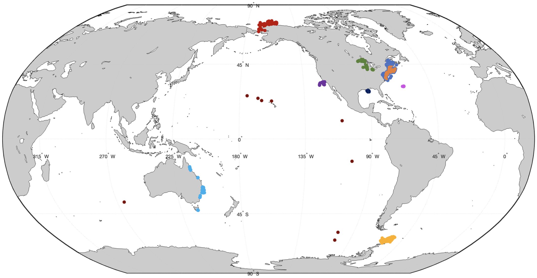
Figure 1. Map of data locations. Data are colored by region with 92 locations in the Arctic (red), 340 locations in the Great Lakes (green), 2,184 locations along the East Coast of the United States (medium blue), 94 samples near Bermuda (magenta), 22 samples along the Gulf of Mexico (dark blue), 428 samples off the coast of California (purple), 151 samples near Antarctica (yellow), 78 samples along the East Coast of Australia (light blue), and 10 samples throughout the rest of the oceans, including near Hawaii (dark red). Samples with matching HPLC data (n = 118) are highlighted in orange.

The discrete sample library contained a variety of wavelength resolutions for absorption parameters. The DAISEA2 algorithm requires an evenly spaced wavelength resolution <5 nm for a given a_nw(λ) input. To simplify the analysis and compare algorithm performance between samples, all absorption data were linearly interpolated to a 1-nm wavelength resolution from 350 nm to 700 nm prior to analysis with DAISEA2. To assess algorithm performance, the library was split into the original development (2,329 spectra) and validation datasets from Grunert et al. (2019). EcoMon and GSO Pier samples were then added to the validation set (total of 1,092 spectra). Performance metrics were not significantly different between development and validation datasets, and all further analysis was conducted on the total library.

On the EcoMon cruises, discrete samples for high-performance liquid chromatography (HPLC) were collected and sent to NASA’s Ocean Ecology Lab to resolve pigment concentrations alongside phytoplankton absorption spectra. Phytoplankton contain a wide variety of pigments that serve photosynthetic and photoprotective purposes. Each of these pigments, and/or sets of pigments, has its own absorption spectrum (Hoepffner and Sathyendranath, 1991, 1993; Chase et al., 2013) and sums to produce total phytoplankton absorption (Supplementary Figure S1). DAISEA2 uses Gaussian decomposition to parse estimated a_ph(λ) into the most likely set of pigment-specific spectra. We compare DAISEA2-retrieved parameters, including a_ph(λ) at a reference wavelength relative to maximum absorption of a given pigment documented in the literature [a_ph(λ_r)], Gaussian peak height, and Gaussian peak area to measured pigments from HPLC for these 118 samples to derive relationships and assess the algorithm’s potential ability to detect pigment composition and concentration from a_ph(λ).

2.2 DAISEA2 algorithm update

The four major updates to DAISEA2 involve (1) the introduction of genetic algorithms to retrieve fitted parameters and associated uncertainty in the form of confidence intervals, (2) adding the option of either an exponential or hyperbolic relationship for a_dg(λ), (3) the ability to process spectra that only extend to 400 nm (AC-S data) rather than requiring absorption be resolved to 350 nm, and (4) evaluating the ability of DAISEA2 to estimate pigment concentrations. We also made small changes to other steps throughout the DAISEA algorithm. While the basic processing steps in Grunert et al. (2019) are followed here, they are outlined again to highlight any changes in the DAISEA2 update.

DAISEA2 takes the input of a_nw(λ) and separates it into its constituent parts of a_ph(λ) and the combined sum of CDOM+NAP absorption [a_dg(λ), m⁻¹]. The approach uses derivative analysis to first estimate a_dg(λ) and then applies Gaussian decomposition to describe the spectral shape of a_ph(λ). Steps described below are outlined in the schematic (Figure 2) to illustrate algorithm workflow.

Figure 2

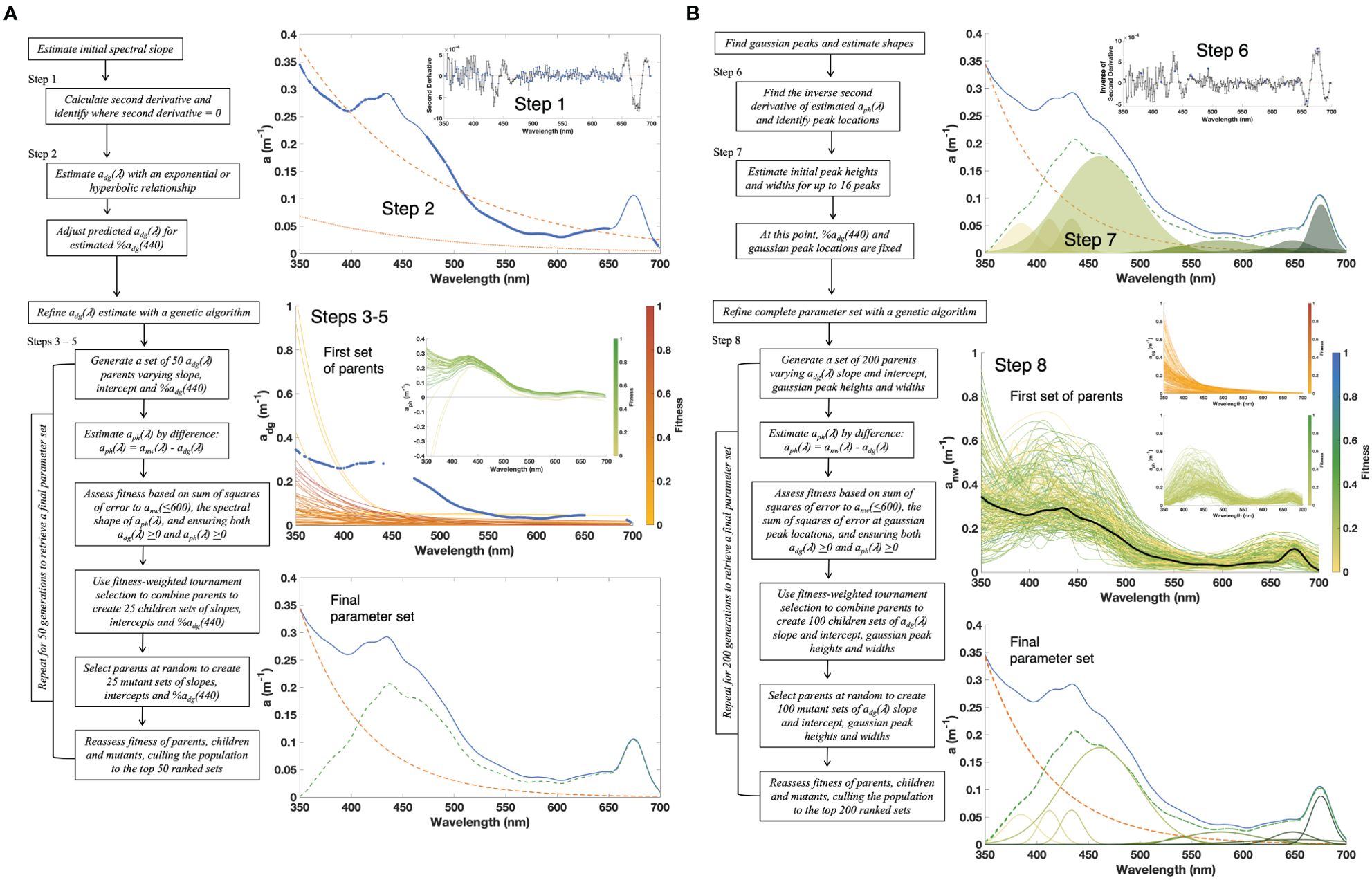
Figure 2. Schematic outlining the processing steps included in DAISEA2, with example figures summarizing each major step.

Step 1

As in DAISEA, the second derivative of a_nw(λ) is used to identify absorption at wavelengths most representative of a_dg(λ) and least influenced by phytoplankton absorption (Equation 1):

$\begin{array}{ll}\frac{d^2{a}_{nw}(\lambda )}{d{\lambda }^2}\approx \frac{a_{nw}({\lambda }_i)-2a_{nw}({\lambda }_j)+ a_{nw}({\lambda }_k)}{\Delta {\lambda }^2}& (1)\end{array}$

where Δλ indicates the wavelength resolution ($\Delta \lambda ={\lambda }_j-{\lambda }_i={\lambda }_k-{\lambda }_j$), λ_i is the wavelength for the current a_nw measurement, λ_j is the wavelength at the i^th+1 a_nw measurement, and λ_k is the wavelength at the i^th+2 a_nw measurement (Tsai and Philpot, 1998). Points where the second derivative is zero or approximately zero are expected to be the least influenced by phytoplankton pigments, as inflection points in the spectra (peaks and troughs associated with pigments) are represented as local maxima and minima in the second derivative spectra (Grunert et al., 2019). The original DAISEA algorithm identified these points as those where the second derivative was less than the median second derivative rounded to one significant digit. This is modified in DAISEA2 to identify inflection points as those falling within$0\pm 1SD(d^2{a}_{nw}(\lambda )/d{\lambda }^2)$. This small change results in fewer selected points along the curve (data not shown). DAISEA2 also explicitly excludes two major regions of the spectrum associated with chl a: 457 nm ± 15 nm and 676 nm ± 15 nm (Chase et al., 2013), as chl a is a ubiquitous pigment associated with phytoplankton (Figure 2, Step 1).

Step 2

Using the points identified in Step 1, an initial estimate of a_dg(λ) is obtained via a non-linear least squares fit to either an exponential (Equation 2) or hyperbolic (Equation 3) relationship:

$\begin{array}{ll}{a}_{nw}(\lambda )=a_{nw}({\lambda }_0)e^{-S(\lambda -{\lambda }_0)}& (2)\end{array}$

where λ₀ is the selected reference wavelength, a_nw(λ₀) is the value of a_nw at the reference wavelength, and S is the spectral slope. DAISEA2 specifies λ₀ as 440 nm. Considering past studies showing strong performance of alternative models for fitting a_g(λ) or a_dg(λ) (e.g., Twardowski et al., 2004; Cael and Boss, 2017), DAISEA2 can alternatively implement the hyperbolic equation of Twardowski et al. (2004):

$\begin{array}{ll}{a}_{nw}(\lambda )=a_{nw}({\lambda }_0)·{(\lambda /{\lambda }_0)}^{-S}& (3)\end{array}$

where λ₀, a_nw(λ₀), and S are defined as for Equation 2. Again, DAISEA2 specifies λ₀ as 440 nm. Note, whether selecting the exponential or hyperbolic relationship, DAISEA2 is a wide-spectrum slope determination across the entire wavelength range and not representative of spectral shape in specific, targeted regions (e.g., 275–295 or 350–400 nm; Helms et al., 2008; Grunert et al., 2018). Applying Equation 2 or Equation 3 yields an initial estimate of a_dg(λ), slope (S_dg, nm⁻¹), and intercept (a_dg(440), m⁻¹). Although the magnitude of S_dg derived from an exponential or hyperbolic relationship is different, the purpose of the parameter is identical and S_dg is used interchangeably to represent either for the remainder of this discussion.

To separate the relative contributions of phytoplankton and CDOM+NAP to total absorption at 440 nm, Grunert et al. (2019) derived an empirical relationship based on their training dataset also applied in DAISEA2 (Equations 4–6). The equations are repeated here for completeness:

$\begin{array}{ll}\%a_{ph}(440)=1.038e^{-0.9257(\frac{a_{nw}(555)}{a_{nw}(680)})}, where \frac{a_{nw}(555)}{a_{nw}(680)}>0.685& (4)\end{array}$

or

$\begin{array}{ll}\%a_{ph}(440)=2.088e^{-1.9460(\frac{a_{nw}(555)}{a_{nw}(680)})}, where \frac{a_{nw}(555)}{a_{nw}(680)}\le 0.685& (5)\end{array}$

and

$\begin{array}{ll}\%a_{dg}(440)=100-\%a_{ph}(440)& (6)\end{array}$

These relationships remained robust in providing fairly accurate and unbiased estimates of absorption to initialize the DAISEA model (Supplementary Figure S2). The estimate of a_dg(440) from Equation 2 or Equation 3 is modified by %a_dg(440) and retrieved a_dg(λ) updated to reflect this absorption magnitude (Figure 2, Step 2).

Steps 3–5

Phytoplankton absorption is then retrieved by difference (Equation 7):

$\begin{array}{ll}{a}_{ph}(\lambda )=a_{nw}(\lambda )-a_{dg}(\lambda )& (7)\end{array}$

At this point, the initial DAISEA algorithm used an iterative process to assess the feasibility of a_ph(λ) and modify S_dg and/or a_dg(440) until a plausible solution was found. DAISEA2 diverges from this approach, instead implementing a genetic algorithm. Genetic algorithms work with entire parameter sets, instead of adjusting the value of each fitted parameter separately, to iteratively reach an optimal solution (Holland, 1975; Houck et al., 1998) and have been used successfully in other optical oceanographic applications (Zhan et al., 2003; Kostadinov et al., 2007). Initial parameter sets are randomly generated to create a group of parents ranked by specified “fitness” criteria. Pairs of parental parameters are selected and combined to create “children” based on ranking; a higher ranking increases the probability of selection. A random subset of parental parameters, independent of rank, is also selected and “mutated” through random percent change. The “parent,” “children,” and “mutant” sets are collectively ranked by fitness, and half the population is culled. This new population becomes the next set of parents. The process is repeated until a fitness threshold is reached or a maximum number of generations is exceeded.

Genetic algorithms were initially designed to work with binary values, requiring parameter sets to be converted into binary strings cut and modified during selection, combination, and mutation (Holland, 1975). Here, we implement a methodology adapted from Houck et al., 1998, who demonstrated that working with values in the real world yielded identical results to binary transformations. In addition to random percent mutation, binary-based genetic algorithms also allow a kind of transpose mutation that exchanges one parameter value for another; for example, the value for a_dg(440) would instead be assigned as S_dg and vice versa. In our case, there is no reason to expect this kind of mutation to yield a feasible parameter set, and we did not include it in the algorithm.

For DAISEA2, the initial parameter set from Step 2 is added to a random set of 49 a_dg(440), S_dg, and %a_dg(440) triplets to generate 50 parents. While parameter sets are randomly generated, limits are placed on a_dg(440), S_dg, and %a_dg(440) to reduce processing time. For both exponential and hyperbolic relationships, a_dg(440) is restricted to between 0 m⁻¹ and input a_nw(440). Slope is restricted to between 0 and 0.03 nm⁻¹ for exponential and 0 to the initial estimate + 4 nm⁻¹ for hyperbolic fits. Finally, %a_dg(440) is restricted to between ±10% of the initial estimate from Equation 6. For each parent set of a_dg(440), S_dg, and %a_dg(440), Equation 2 (exponential) or Equation 3 (hyperbolic) and Equation 7 are applied to estimate a_dg(λ) and a_ph(λ). Fitness is assessed as (Equation 8)

$\begin{array}{ll}F=(\frac{1}{f_1}+f_2+f_3)·f_4& (8)\end{array}$

where f₁ (Equation 9) is the sum of squares of error up to 600 nm:

$\begin{array}{ll}{f}_1=\sum _{\lambda ={\lambda }_{min}}^{600nm}{[a_{nw}(\lambda )-\widehat{a_{nw}}(\lambda )]}^2& (9)\end{array}$

Since the purpose of Steps 3–5 is to estimate a_dg(λ), we chose to minimize error up to 600 nm, rather than 700 nm, to avoid the influence of chl a at red wavelengths, often visible as a peak in a_nw(λ). f₂ is a true/false metric that assesses the shape of the phytoplankton spectra (Equation 10). Since a_ph(λ) is obtained by difference, it is possible to have residual influence of a_dg(λ) if estimated slope or intercept is inaccurate. As in Grunert et al. (2019), we considered phytoplankton spectra to be reasonable if

$\begin{array}{ll}{f}_2({\lambda }_{min}\le 350nm)=1 when \frac{\widehat{a_{ph}}(350)}{\widehat{a_{ph}}(440)}\le 1.5, and 0 otherwise& (10)\end{array}$

or, for spectra, such as those recorded for the AC-S (Equation 11), with λ_min = 400nm:

$\begin{array}{ll}{f}_2({\lambda }_{min}=400nm)=1 when \frac{\widehat{a_{ph}}(400)}{\widehat{a_{ph}}(440)}\le 1.2, and 0 otherwise& (11)\end{array}$

Both f₃ (Equation 12) and f₄ (Equation 13) are true/false metrics ensuring estimated a_dg(λ) and a_ph(λ) are positive:

$\begin{array}{ll}{f}_3=1 when \frac{{\sum }_{\lambda ={\lambda }_{min}}^{690nm}\widehat{a_{dg}}(\lambda )>0}{690-{\lambda }_{min}}=1, and 0 otherwise& (12)\end{array}$

$\begin{array}{ll}{f}_4=1 when \frac{{\sum }_{\lambda ={\lambda }_{min}}^{690nm}\widehat{a_{ph}}(\lambda )>0}{690-{\lambda }_{min}}=1, and 0 otherwise& (13)\end{array}$

Note that it is a requirement of the algorithm that a_ph(λ) be positive [in other words, a_dg(λ) must be less than a_nw(λ) for all wavelengths]; retrieving negative phytoplankton absorption will result in a fitness of zero. This requirement is slightly relaxed for a_dg(λ) as f₃ simply reduces fitness rather than canceling it, as a_dg(λ) at wavelengths greater than 600 nm is often near zero. Both metrics only consider wavelengths less than 690 nm as a_nw(λ) is close to zero at higher wavelengths, making it difficult to meet the f₃ and f₄ criteria. During development, extending f₃ and f₄ to the full spectrum resulted in algorithm failure for many of the spectra in the dataset library (data not shown).

The 50 parental parameter sets are ranked by fitness from highest to lowest. Tournament selection is used to generate children: 25 pairs of parents are randomly drawn, with replacement, weighted by fitness, from the population. Each pair is combined to generate a child parameter set using the mean value of the two parents. Mutation is performed on an additional 25 randomly selected parents, without replacement, ignoring rank. Each parameter in the mutation set is modified by a randomly generated percentage up to ±20% of its initial value. Fitness is reassessed with Equation 8 for the combined set of parents, children, and mutants. The 50 highest ranked individuals are selected as the next generation of parents. The genetic algorithm runs for 50 generations to retrieve updated estimates of a_dg(440), S_dg, and %a_dg(440). DAISEA2 repeats the genetic algorithm 10 times to generate an ensemble for each of the three parameters. The median ensemble values of a_dg(440), S_dg, and %a_dg(440) are utilized in Steps 6 and 7 (Figure 2, Steps 3–5).

Steps 6 and 7

Gaussian decomposition is applied to a_ph(λ) estimated after Steps 3–5 to retrieve the number and location of pigment peaks. Peak locations are not assumed a priori. Instead, peaks are found by applying second derivative analysis to the a_ph(λ) signal. These steps closely follow the original DAISEA algorithm with some updates. The second derivative of a_ph(λ) is first smoothed by a Savitzky-Golay filter with a 9-nm window to reduce the potential for identifying noise-related peaks. The signal is then inverted, and local maxima are detected where the first derivative is zero. This creates an initial set of potential peak locations, heights, and widths as (Equation 14)

$\begin{array}{ll}{ɡ}_i={\varphi }_i{e}^{-\frac{{(\lambda -{\mu }_i)}^2}{2{\sigma }_i}}& (14)\end{array}$

where μ (nm) is the location of the peak center on the spectrum, σ (nm) is peak width, and ϕ (m⁻¹) is peak height. Peaks with σ <5 nm are considered noise and removed as peak widths associated with individual pigments or groups of pigments range from 10 nm to 53 nm (Hoepffner and Sathyendranath, 1993; Bricaud et al., 2004; Chase et al., 2013).

At this point, retrieved peak height relates to the magnitude of the second derivative rather than phytoplankton absorption. Thus, Gaussian peaks are next mapped onto a_ph(λ). Peak height is used as a proxy for peak importance and mapping proceeds from the tallest to the shortest peak. The process is iterative; as each peak is mapped, the signal for that peak is removed from a_ph(λ) before mapping the next peak. For each successive μ_i, peak height is defined as 90% of remaining a_ph(λ) at that wavelength (Equation 15):

$\begin{array}{ll}{\varphi }_i(\lambda )=0.90\left(a_{ph}(\lambda )-\sum _{i=1}^n{\varphi }_i{e}^{-\frac{{(\lambda -{\mu }_i)}^2}{2{\sigma }_i}}\right)& (15)\end{array}$

where n indicates the total number of peaks found. This is a slight change from the original DAISEA, that assigned 100% of a_ph(λ) for each successive peak instead of 90%. Due to the additive nature of the process, it is possible to retrieve peaks with negative heights. As with the original DAISEA, negative peaks are excluded, and remaining peaks ordered by height as a proxy of importance. The peak set is then trimmed to a maximum of 16.

Here, DAISEA2 diverges from the original DAISEA by checking peak locations against eight known peaks from the literature. Specifically, DAISEA2 looks for peak matches against the most common pigments associated with phytoplankton (Table 1, Chl a and b) and attempts to add a peak location if none exists within ±10 nm. Any peaks added in this step are assigned a peak height equal to a_ph(λ) after Equation 15 is applied. Again, peaks with negative heights are removed, remaining peaks are ordered by importance, and only 16 are retained. Thus, peaks added from Table 1 during this step can still be excluded (Figure 2, Steps 6 and 7).

Table 1

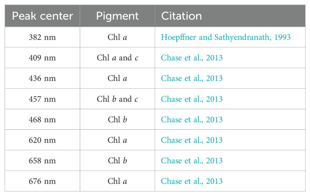
Table 1. Peak locations from the literature associated with the most common phytoplankton pigments, Chl a and b.

Step 8

The final set of μ, ϕ, and σ from Step 7 along with a_dg(440), S_dg, and %a_dg(440) from Step 5 are used to create limits for a final genetic algorithm optimizing the parameter set. Both the number and locations (μ) of Gaussian peaks are fixed and not allowed to vary during this final step. This is a change from the original DAISEA where peak locations could vary by ±5 nm. The estimated contribution of a_dg at 440 nm [%a_dg(440)] is also kept constant. Data are fit to a combination of Equations 2 and 14 (Equation 16) if an exponential relationship is specified for a_dg(λ):

$\begin{array}{ll}{a}_{nw}(\lambda )=\%a_{dg}({\lambda }_0)·a_{nw}({\lambda }_0)e^{-S(\lambda -{\lambda }_0)}+\sum _{i=1}^n{\varphi }_i{e}^{-\frac{{(\lambda -{\mu }_i)}^2}{2{\sigma }_i}}& (16)\end{array}$

or to Equations 3 and 17 if a hyperbolic relationship is used:

$\begin{array}{ll}{a}_{nw}(\lambda )=\%a_{dg}({\lambda }_0)·a_{nw}({\lambda }_0)·{(\lambda /{\lambda }_0)}^{-S}+\sum _{i=1}^n{\varphi }_i{e}^{-\frac{{(\lambda -{\mu }_i)}^2}{2{\sigma }_i}}& (17)\end{array}$

For the genetic algorithm, an initial parent population of 200 sets of ϕ, σ, a_dg(440), and S_dg are generated from a combination of 100 random parameter sets and 100 parameter sets within up to a random ±50% of their input values. While this means the initial parent population is not entirely random, it leverages the effort from Steps 1 to 7 to greatly reduce final computation time and provide reasonable constraints for the parameter space based on observed data. The following limits are imposed on all 200 parents: ϕ_i is allowed to vary between 0 m⁻¹ and a_nw(μ_i), σ between 5 nm and 50 nm, a_dg(440) between 0 m⁻¹ and a_nw(440), and S_dg between −0.002 and +0.003 nm⁻¹ of its input value for exponential relationships and between −2 and +5 nm⁻¹ of its initial value for hyperbolic fits. Grunert et al. (2019) detail the reasoning behind asymmetrical limits on S_dg in their discussion.

Using Equation 2 (exponential) or Equation 3 (hyperbolic) and Equation 7, estimates of a_dg(λ) and a_ph(λ) are calculated for each parent parameter set. Fitness is assessed as (Equation 18)

$\begin{array}{ll}F=\frac{1/f_5}{\text{max}(1/f_5)}+\frac{1/f_6}{\text{max}(1/f_6)}+f_3+f_4& (18)\end{array}$

where f₅ is the sum of squares of error over the entire wavelength range (Equation 19):

$\begin{array}{ll}{f}_5=\sum _{\lambda ={\lambda }_{min}}^{\lambda ={\lambda }_{max}}{[a_{nw}(\lambda )-\widehat{a_{nw}}(\lambda )]}^2& (19)\end{array}$

and f₆ is the sum of squares of error at the Gaussian peak locations (Equation 20):

$\begin{array}{ll}{f}_6=\sum _{i=1}^n{[a_{nw}({\mu }_i)-\widehat{a_{nw}}({\mu }_i)]}^2& (20)\end{array}$

Both f₅ and f₆ are scaled to the maximum value so they range between 0 and 1, making them of equal importance to fitness. Parameters f₃ and f₄ are as defined above during Steps 3–5 in Equations 12 and 13: true/false values ensuring a_dg(λ) and a_ph(λ) are positive for wavelengths <690 nm.

The 200 parental parameter sets are ranked by fitness from highest to lowest. As in Steps 3–5, tournament selection is used to generate children: 100 pairs of parents are randomly drawn, with replacement, weighted by fitness, from the population. Each pair is combined to generate a child parameter set using the mean value of the two parents. Mutation is then performed on an additional 100 randomly selected parents, without replacement, ignoring rank. Each parameter in the mutant set is modified by a randomly generated percentage up to ±10% of its initial value. Fitness is reassessed with Equation 18 for the combined set of parents, children, and mutants. The 200 highest ranked individuals are selected as the next generation of parents.

The genetic algorithm runs for 200 generations or for a minimum of 100 generations, and then until f₅< 0.002. During development, we found that the genetic algorithm either converged rather quickly on a parameter set (within 200 generations) or that it would take 1,000s of generations to reach a consistent solution. The limits described here balance computation time with the desire for an accurate retrieval. DAISEA2 repeats the genetic algorithm 10 times to generate ensembles for ϕ, σ, a_dg(440), and S_dg. Final parameter estimates are returned as the median of the ensemble. Error is assessed as the minimum and maximum ensemble value for each parameter. Final estimates of a_dg(λ) and a_ph(λ) are returned utilizing Equation 2 (exponential) or Equation 3 (hyperbolic) and Equation 7.

2.3 Efficiency and runtime

DAISEA2 was run on a Mac Pro (2019), 3.2 GHz, 16-core Intel Xenon W with 96 GB of RAM. Runtimes for DAISEA2 were independent of a_dg model choice (exponential/hyperbolic) and were bimodal with peaks at 8–9 s and 16–17 s per curve (data not shown). Minimum and maximum runtimes were <1 s and 25 s, respectively, with 24% of the dataset falling < 10 s and 61% of the dataset falling between 10 s and 20 s. Full runs for all 3,421 spectra took 13h utilizing a single processor. One of the goals of DAISEA2 was to create an algorithm that enables utilization of in-situ profiles, continuous underway flowthrough, or fixed-point time series absorption measurements that often only resolve a_nw(λ), such as those taken with an AC-S. We have collected such a dataset ourselves, amassing 34,031 AC-S spectra at both a fixed-point time series on a pier and from underway measurements on cruises along the eastern coast of the United States. We estimate it would take 6 days to analyze this entire dataset with a single processor.

To have a sense of the effort required to apply DAISEA2 to a satellite data product, we took a single global PACE Level 3 monthly global product and multiplied the number of pixels with data by the relative runtime spread for our DAISEA2 analysis. We estimate that it would take 555 days to process the 3,226,628 pixels with values in this scene using a single processor. This can be dramatically reduced by utilizing computing power commonly available today: allocating 15 of the 16 cores on our Mac Pro would cut this runtime down to 37 days. We expect that a computing cluster and parallel computing techniques that are increasingly available to the community would enable DAISEA2 to be efficient enough to process PACE data. Future efforts will focus on avenues for improving efficiency, particularly when paired with computationally intensive inversion schemes.

2.4 Data analysis

We assessed the performance of DAISEA2 by considering performance across eight broad classes of optical conditions. Classes were defined by the percent contribution of a_ph at 440 nm [%a_ph(440)], ranging from 0% to >70% in increments of 10%, with n = 1329 (<10%), 346 (10%–20%), 460 (20%–30%), 425 (30%–40%), 287 (40%–50%), 230 (50%–60%), 177 (60%–70%), and 136 (>70%) spectra, respectively. This approach considers the relative contribution of phytoplankton pigments to the overall absorption signal and follows delineation in Grunert et al. (2019). Performance was assessed using several common performance metrics (Seegers et al., 2018), including root-mean-square difference (RMSD) (Equation 21), normalized RMSD (NRMSD) (Equation 22), bias (Equation 23), and mean absolute difference (MAD) (Equation 24) using the following expressions:

$\begin{array}{ll}RMSD= \sqrt{\frac{{\sum }_{i=1}^n{(x_i^{estimated}-x_i^{observed})}^2}{n}}& (21)\end{array}$

$\begin{array}{ll}NRMSD (\%)=\frac{RMSD}{x_{max}^{observed}-x_{min}^{observed}}\times 100& (22)\end{array}$

$\begin{array}{ll}Bias= \frac{1}{n}\sum _{i=1}^n(x_i^{estimated}-x_i^{observed})& (23)\end{array}$

$\begin{array}{ll}MAD= \frac{{\sum }_{i=1}^n(\left|x_i^{estimated}-x_i^{observed}\right|)}{n}& (24)\end{array}$

Additionally, we considered whether a_ph(λ) or a_dg(λ) was retrievable by calculating the absolute difference in the opposing metric and comparing this value to the observed value, following Grunert et al. (2019). The premise for this approach is that if the uncertainty in a retrieved parameter is larger than the value of the other parameter, then we cannot retrieve that parameter with adequate confidence. Finally, Bayes factors (BF₁₀, unitless) were also calculated to assess fit significance (Wetzels and Wagenmakers, 2012). Bayes factors represent the likelihood that modeled results better represent observed data relative to an alternative model, with a BF₁₀ = 2 indicating the model is twice as likely to explain observed data than an alternative model, with a BF₁₀ ≥ 3 used as a threshold of significance (Wetzels and Wagenmakers, 2012).

3 Results

DAISEA2 is a revision of the original DAISEA algorithm (Grunert et al., 2019) and includes improvements in performance as highlighted below while also providing uncertainty estimates for all retrieved components. These retrieved components include spectral absorption coefficients and slope parameters associated with exponential or hyperbolic models representing a_dg(λ), spectral absorption coefficients for a_ph(λ), and Gaussian components used to model phytoplankton pigment absorption (including ϕ, μ, and σ as outlined in Equations 16, Equation 17). Additionally, we evaluated the ability of DAISEA2 to estimate HPLC pigment concentrations estimated from a_ph(λ_r), where λ_r is the corresponding wavelength for extracted pigment peak absorption, Gaussian peak height, and Gaussian peak area for Gaussian components corresponding to a particular pigment. The DAISEA2 algorithm performance followed similar broad trends to the performance of the initial DIASEA algorithm (Grunert et al., 2019), including strong spectral agreement between observed and modeled a_ph(λ) and a_dg(λ) across a range of optical conditions, from waters dominated by a_dg(λ) to waters dominated by a_ph(λ) (Figure 3).

Figure 3

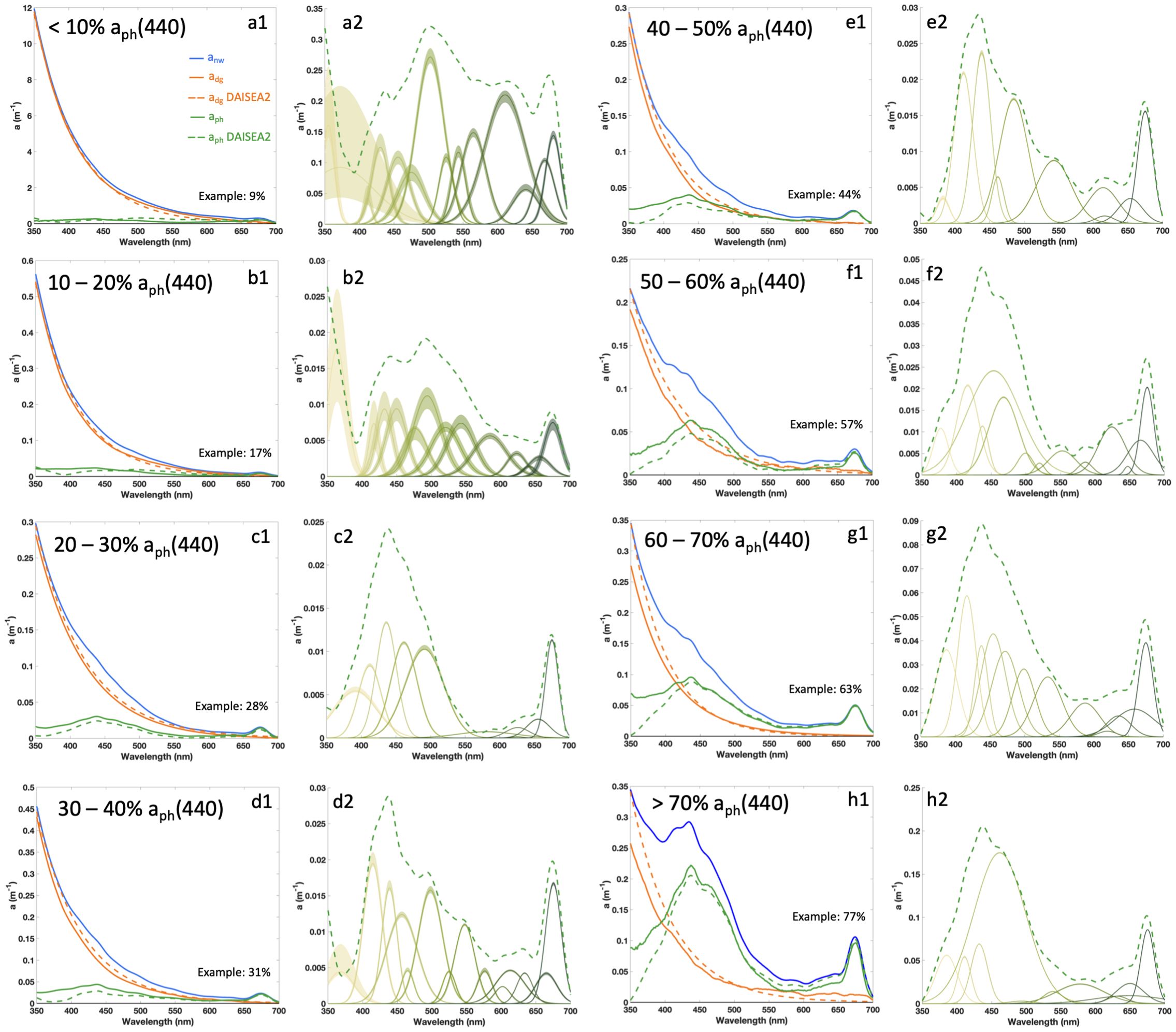
Figure 3. Example retrievals of a_dg(λ), a_ph(λ), and associated Gaussian decomposition with DAISEA2. For a1-h1, solid lines represent measured data and dashed lines show modeled results. In a2-h2, shaded areas for Gaussian decomposition represent outer bounds on peak height and width from the genetic algorithm, with the dashed line corresponding to modeled a_ph(λ). Measured spectra were grouped by percent contribution of a_ph(λ) at 440 nm. An example for each bin was selected as the spectra closest to the median residual a_ph(λ) except for the <10% group, which was selected by hand.

DAISEA2 improved spectral retrieval of a_ph(λ) and a_dg(λ) for all sites relative to DAISEA, with significant improvements in the retrievability of a_ph(λ) and a_dg(λ), particularly at longer wavelengths relative to the original model (Figure 4). Notably, from 550 nm to 700 nm, no more than 80% of sites saw a_ph(λ) retrievable in DAISEA, while the majority of wavelengths from 550 nm to 700 nm were well above 80% retrievable for spectra with % a_ph(440) > 30 using DAISEA2. These gains were made while maintaining or slightly improving the retrievability of a_dg(λ) for all classes outside of %a_ph(440) < 10. The retrievability and NRMSE were lower for a_dg(λ) at wavelengths greater than 550 nm, following an approximately exponential decrease and increase, respectively (Figure 4); this apparently contradictory behavior is due to relatively large magnitudes of a_ph(λ) for many of these sites and the relatively small magnitude of a_dg(λ) at corresponding wavelengths. Inland and coastal sites dominated this class, where a_ph(λ) magnitude was often quite large relative to more oceanic sites, but CDOM absorption was also extremely high at 440 nm (values in excess of 1 m⁻¹) for many of these data, resulting in the low relative value of %a_ph(440).

Figure 4

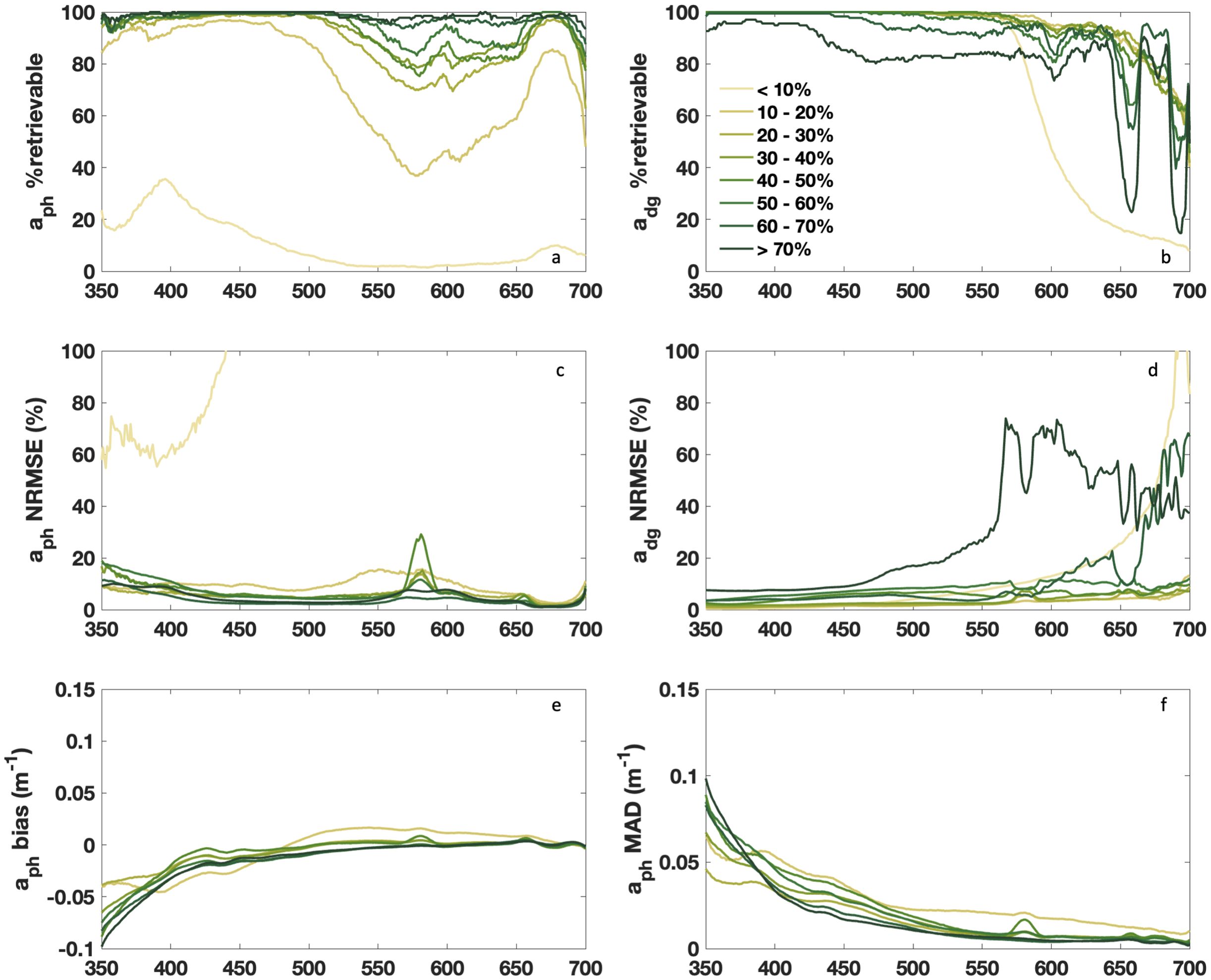
Figure 4. Spectral performance for DAISEA2 retrieval of a_ph(λ) and a_dg(λ) using an exponential model for a_dg(λ) following Equations 21–24 in Section 2.3. Data were grouped by percent contribution of a_ph(λ) at 440 nm as indicated in the legend for (a) aph % retrievable, (b) adg % retrievable, (c) aph NRMSE, (d) adg NRMSE, (e) aph bias and (f) aph MAD. Spectral performance using a hyperbolic model for a_dg(λ) can be found in Supplementary Figure S3.

Normalized RMSE was lower for all classes relative to DAISEA, including considerable decreases in NRMSE <550 nm for a_dg(λ) (Figure 4). In DAISEA, there was broad elevation in NRMSE from ~500 nm to 650 nm, while DAISEA2 has limited NRMSE to a local spike near 585 nm, indicating difficulty in fitting Chl a and c absorption at this spectral location for a subset of samples (Figure 4). Across classes, a_ph(λ) below 400 nm shows a negative bias of −0.05 to 0.1 m⁻¹ and elevated MAD below 500 nm, consistent with the algorithm systematically allocating UV absorption to a_dg(λ) instead of a_ph(λ) (Figures 4E, F). This is in contrast to DAISEA, which typically overestimated the contribution of a_ph(λ) for lower %a_ph(440) spectra and underestimated the contribution of a_ph(λ) for higher %a_ph(440) spectra at shorter wavelengths. Algorithm performance was broadly similar when using the hyperbolic model to represent a_dg(λ), except for generally improved retrievability of a_ph(λ) and a distinct spectral bias in a_ph(λ) below 450 nm represented by overestimations of pigment absorption between 400 and 500 nm (Supplementary Figure S3). The improved spectral performance of the hyperbolic model represents its ability to adequately constrain the relatively singular spectral shape of CDOM absorption from 400 nm to 700 nm, which is primarily due to charge transfer effects with a rapid degradation in fitting performance near 350 nm when the spectral complexity of a_dg(λ) increases considerably. The slightly improved performance of the hyperbolic model on CDOM absorption for spectral regions dominated by visible wavelengths (e.g., ~400 nm to 700 nm) has been previously described (Twardowski et al., 2004) and is supported by a higher spectral win rate here (Supplementary Figure S4; Seegers et al., 2018). However, as a hyperbolic model approaches infinity in finite time, the edge region of any UV retrieval is expected to rapidly deteriorate relative to an exponential model. To be consistent with the accepted community use of the exponential model, we prioritize the presentation of the exponential model here but include identical figures for the hyperbolic model performance as supplementary figures to provide a balanced narrative of strengths and limitations to each approach. It should be noted that some improvements in performance were anticipated based on stricter quality control of data used in the evaluation of DAISEA2 relative to those used in DAISEA (see Section 2.1). Overall, DAISEA2 showed an average spectral improvement of +15% retrievability of a_ph(λ), reduced NRMSE of 7.5% and 4.8% for a_ph(λ) and a_dg(λ), respectively, and a reduction in MAE of 0.015 for a_ph(λ). The average retrievability of a_dg(λ) was maintained, and average bias was near zero due to the divergence in bias as described above (data not shown).

DAISEA2 remains challenged in resolving the UV contribution of phytoplankton, largely attributed to inequality constraints used to resolve the contribution of a_dg(λ) (Equation 10; Figure 2) and the irregular contributions of UV-absorbing pigments, including Chl a absorption at 382 nm and mycosporine-like amino acids (MAAs). MAAs, in particular, remain poorly constrained, in part due to databases offering only the wavelength of peak absorption or absorption spectra specific to unknown MAAs or a phytoplankton species and not a compound, and are not parameterized in past approaches that model a_ph(λ) with component pigments (Hoepffner and Sathyendranath, 1993; Sinha et al., 2007; Piiparinen et al., 2015; Vale, 2015; Grunert et al., 2019). These challenges are clear in the systematic bias toward underestimating a_ph(λ) below 400 nm (Figure 4). Generally, algorithm performance was more challenged at shorter wavelengths, as seen in relative MAD values and bias (Figure 4). This was attributed to limitations in defining when a_ph(λ) can be expected to increase or maintain its magnitude at UV wavelengths. This knowledge gap remains in the literature, including when and where MAAs are expected and when Chl a absorption at 382 nm can be expected to be elevated. Presumably, broader knowledge on these spectral characteristics within the community would contribute to an improved understanding of phytoplankton physiology from hyperspectral, UV-observing remote sensing instruments.

Spectral fitting by DAISEA2 is quite robust, as evidenced by consistent and relatively unbiased fitting of S_dg (Figure 5; Supplementary Figure S5) and consistent retrieval of phytoplankton pigment absorption features and good agreement with reconstruction of a_ph(λ) (Figures 3, 6; Supplementary Figure S6). Gaussian components were identified as consistent with known pigment absorption locations >80% of the time, with a significant portion of “unclassified” pigments, or identified peaks that did not agree with established pigment locations in the literature, affiliated with published locations of MAAs (16% of unfitted peaks for DAISEA2 using an exponential model for a_dg(λ) (Supplementary Figure S6; Sinha et al., 2007; Piiparinen et al., 2015; Vale, 2015).

Figure 5

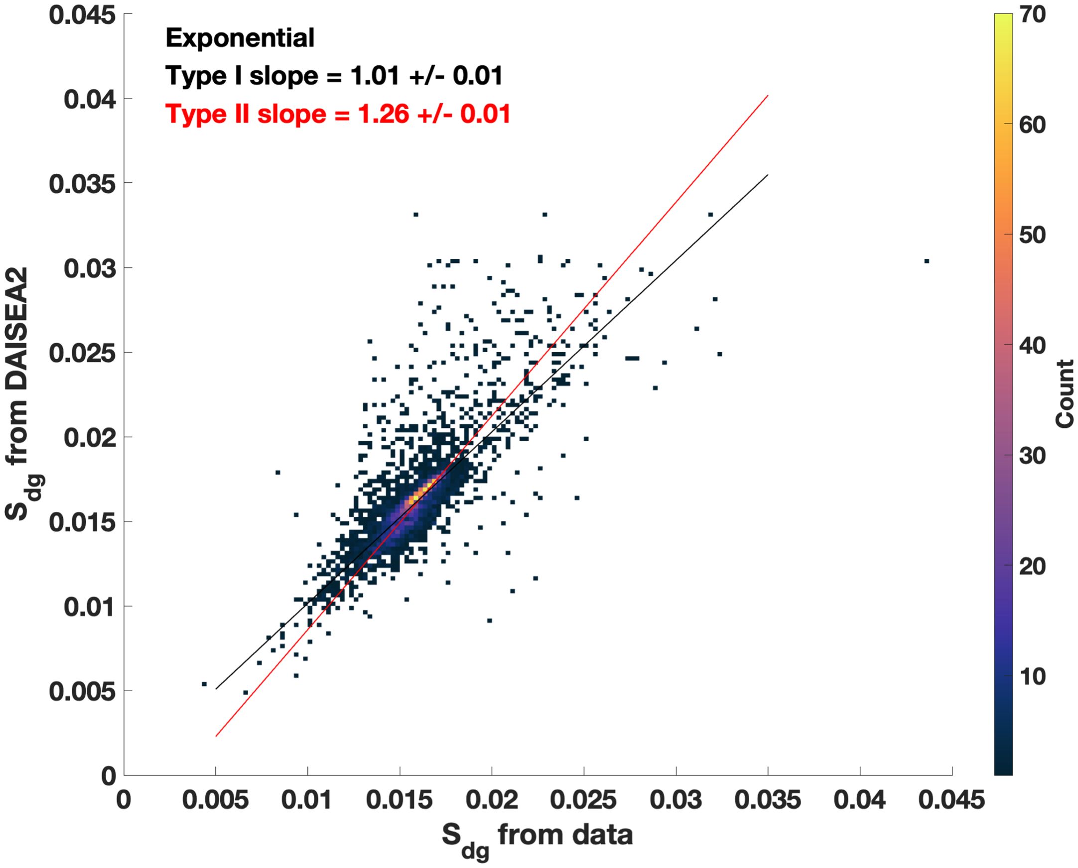
Figure 5. Spectral slope from 350 nm to 700 nm (S_350:700) retrieved from measured a_dg(λ) versus modeled a_dg(λ) with DAISEA2 using an exponential relationship. Across the entire dataset, 71% of modeled S_350:700 fall within ±0.001 of S_350:700 retrieved directly from measured data. Slopes retrieved using a hyperbolic model can be found in Supplementary Figure S4.

Figure 6

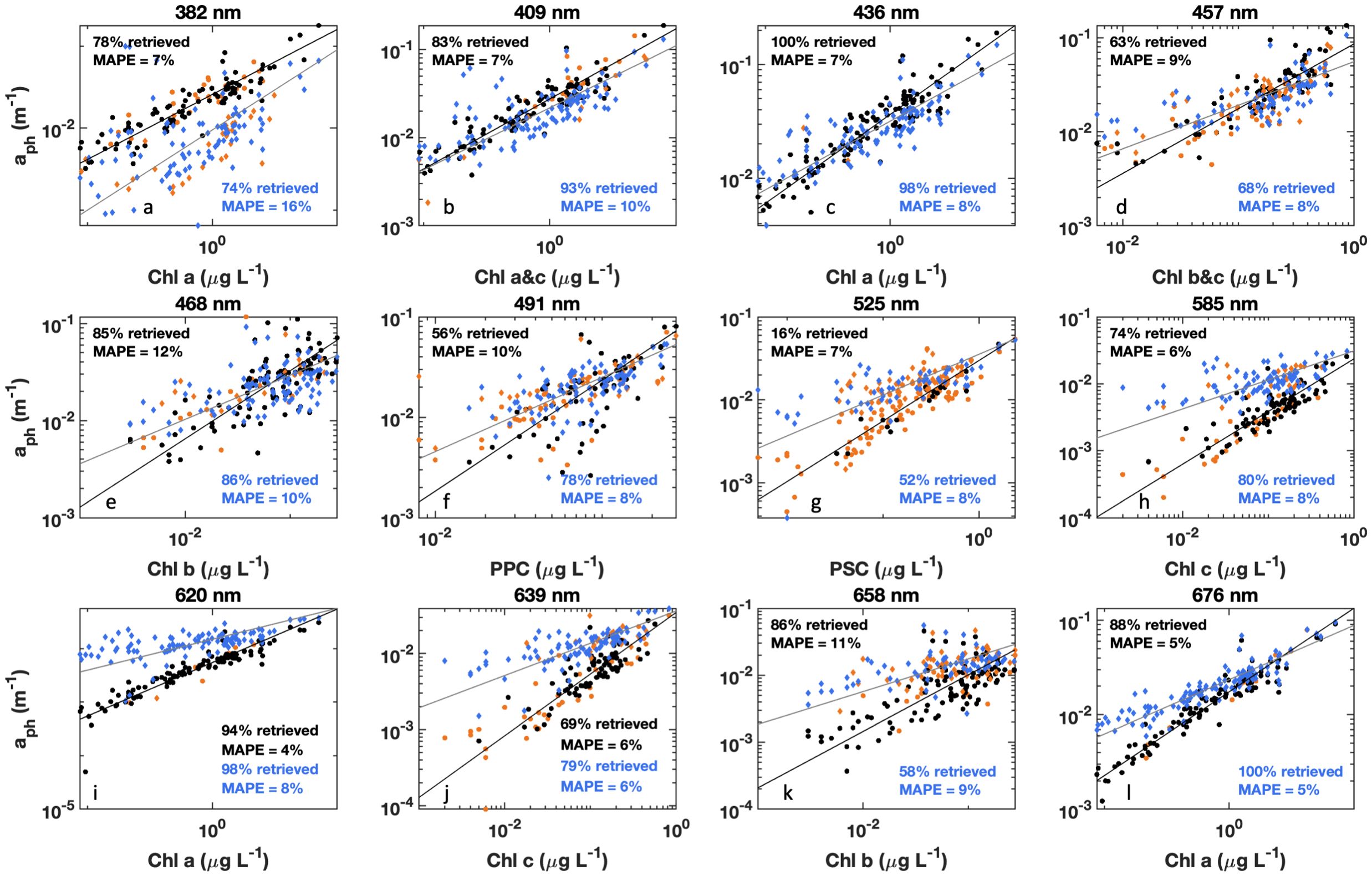
Figure 6. HPLC pigment concentrations vs. a_ph(λ) at associated wavelengths for (a) Chl a, (b) Chl a&c, (c) Chl a, (d) Chl b&c, (e) Chl b, (f) photoprotective carotenoids (PPC), (g) photosynthetic carotenoids (PSC), (h) Chl c, (i) Chl a, (j) Chl c, (k) Chl b, and (l) Chl a, for either measured (circles) or modeled (diamonds) data presented. For measured data, Steps 6 and 7 of DAISEA2 were performed on a_ph(λ) to retrieve initial Gaussian peaks. These were then further refined by a genetic algorithm for Gaussian peaks only. For modeled data, Gaussian peaks were retrieved during decomposition of a_nw(λ) using an exponential relationship for a_dg(λ) with the full DAISEA2 model. For both measured (black) and modeled (blue) analysis, Gaussian peaks within ±10 nm were considered matched to pigment locations. Orange symbols indicate samples where Gaussian decomposition did not retrieve an associated peak. Black (measured) and blue (modeled) lines are a Type II regression of pigment concentration vs. retrieved a_ph(λ) with mean absolute percent error indicated in the subplot text.

HPLC phytoplankton pigment concentrations are well correlated with the magnitude of observed a_ph(λ) at spectral locations associated with those pigments in the literature, referred to here as a_ph(λ_r), and DAISEA2 reliably retrieved pigments at these spectral locations (Table 2; Figure 6). All four absorption peaks at visible wavelengths associated with Chl a were retrieved greater than 90% of the time, including 100% retrieval of the Chl a absorption peak at 676 nm with DAISEA2. Absorption at 382 nm associated with Chl a was retrieved 75% of the time when an exponential model was used for a_dg(λ) (Figure 6) and 86% of the time when a hyperbolic model was used (data not shown), consistent with improved retrieval of a_ph(λ) at UV wavelengths when using a hyperbolic model to fit a_dg(λ). Overall, pigment concentrations displayed MAPE of 4%–12% when related to observed a_ph(λ_r) at wavelengths corresponding with those published in the literature and displayed MAPE of 5%–16% relative to modeled a_ph(λ_r). Relationships between HPLC pigment concentrations and corresponding Gaussian peak height notably decreased when applying Gaussian decomposition and the genetic algorithm to observed a_ph(λ), but improved for modeled Gaussian peak height using DAISEA2 on a_nw(λ) (Table 3, Figure 7). This was a surprising finding; however, ultimately, it indicates that total pigments or the spectral absorption of pigments considered here is underrepresented, both within the literature considered here informing the construction of DAISEA and within the model implementation. If this were not the case, we would expect a bias in pigment relationships, both within observed and modeled a_ph(λ) variables and HPLC pigments. The underrepresentation of phytoplankton pigments and/or spectral features is also supported by significantly larger MAPE between HPLC pigments and Gaussian peak areas used to reconstruct a_ph(λ), indicating an overallocation of absorption to individual pigment peaks (Supplementary Figure S7). Ultimately, DAISEA2 introduced 0%–9% error in pigment relationships when relating pigment concentration to a_ph(λ_r), with reductions in MAPE of up to 2% also observed (Table 2), and DAISEA2 ultimately reduced error in the relationship between pigment concentration and Gaussian peak height by 0%–11% for all pigments except the 676 nm Chl a peak, where MAPE increased by 1% (Table 3). Overall relationships were similar when using a hyperbolic model to fit a_dg(λ) (data not shown).

Table 2

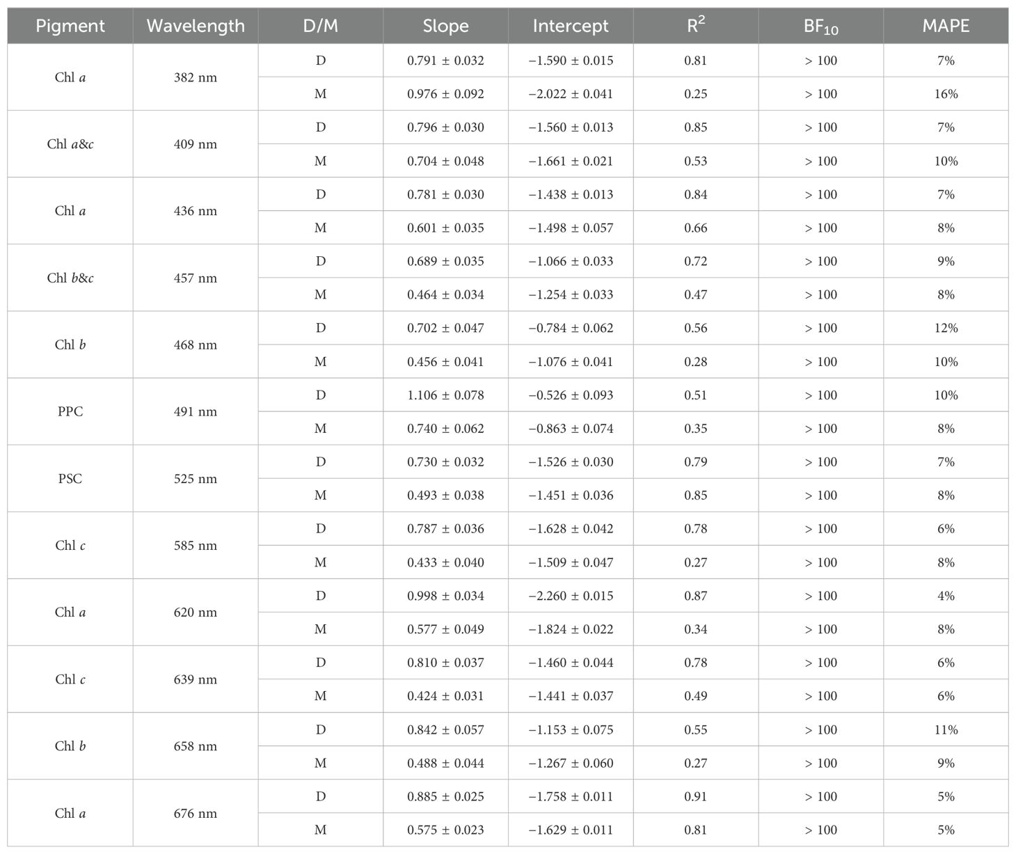
Table 2. Parameters (slope and intercept) along with fit metrics for a Type II linear fit of pigments vs. a_ph(λ) performed on log-transformed data. Results are shown for Gaussian decomposition of both measured (D) and modeled (M) a_ph(λ).

Table 3

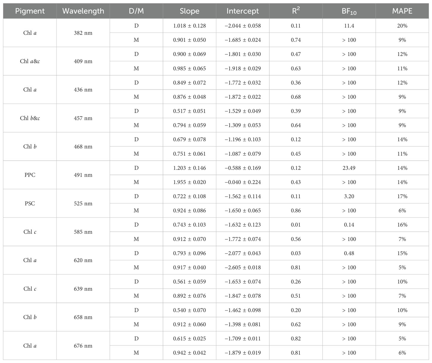
Table 3. Parameters (slope and intercept) along with fit metrics for a Type II linear fit of pigments vs Gaussian peak height performed on log-transformed data. Results are shown for the Gaussian decomposition of both measured (D) and modeled (M) a_ph(λ).

Figure 7

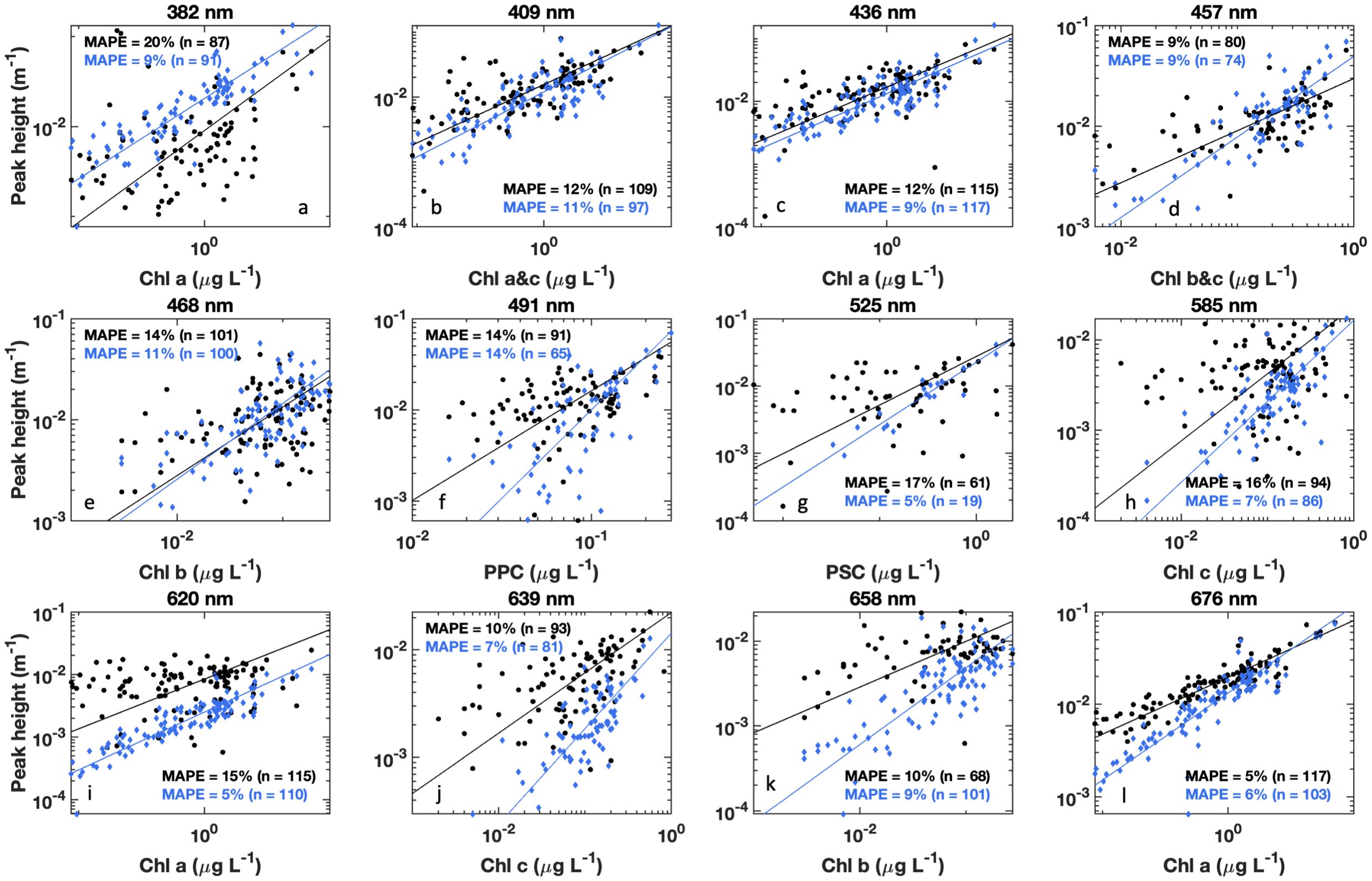
Figure 7. HPLC pigment concentrations vs. modeled Gaussian peak height at associated wavelengths for (a) Chl a, (b) Chl a&c, (c) Chl a, (d) Chl b&c, (e) Chl b, (f) photoprotective carotenoids (PPC), (g) photosynthetic carotenoids (PSC), (h) Chl c, (i) Chl a, (j) Chl c, (k) Chl b, and (l) Chl a, for either measured (black circles) or modeled (blue diamonds) data. For measured data, Steps 6 and 7 of DAISEA2 were performed on a_ph(λ) to retrieve initial Gaussian peaks. These were then further refined by a genetic algorithm for Gaussian peaks only. For modeled data, Gaussian peaks were retrieved during decomposition of a_nw(λ) using an exponential relationship for a_dg(λ) with the full DAISEA2 model. For both measured and modeled analysis, Gaussian peaks within ±10 nm were considered matched to pigment locations. Black (measured) and blue (modeled) lines are a Type II regression of pigment concentration vs. peak height with mean absolute percent error for log transformed data indicated in the subplot text.

We also considered the impact of signal uncertainty and wavelength resolution on the performance of DAISEA2 in anticipation of application to inversion approaches that would provide estimates of a_nw(λ) with varying degrees of error. Noise was randomly introduced at each wavelength in every input spectrum in increments from ±5% to ±20%. Resultant “noisy” DAISEA2 a_ph(λ) and a_dg(λ) were evaluated relative to results with original input data and evaluated against observed a_ph(λ) and a_dg(λ) (Figures 8 and 9). Small errors added to input a_nw(λ) resulted in increasing percent error for both a_ph(λ) and a_dg(λ) when the contribution of a_ph(440) was < 10% (Figure 8A). This was expected, as the magnitude of absorption for these spectra was generally quite large, so small percent errors propagated into significant variability in input magnitude and hindered the ability of DAISEA2 to deconstruct the signal into component IOPs. For increasing error in groups where a_ph(440) represented a larger contribution, error was spectrally variable (Figures 8B–H). Consistent with a bias in underestimating a_ph(λ) at UV wavelengths, estimation of a_ph(λ) improved with the addition of random error at UV wavelengths (Figure 8). Random error is generally not spectrally smooth and resulted in the allocation of a_nw(λ) signal to a_ph(λ) instead of a_dg(λ). At visible wavelengths, absolute error tended to increase with increasing noise; however, ultimately random noise was better fit by Gaussian components than an exponential signal, resulting in an overall increase in estimated a_ph(λ) and Gaussian components. For a_dg(λ), noise tended to result in increasing error at wavelengths below ~500–550 nm and decreasing error at wavelengths above 550 nm, consistent with the mechanisms driving a_ph(λ) trends described previously (Figure 9). For most spectra, moving from a spectral resolution of 5 nm to 1 nm was most important at UV wavelengths when estimating a_ph(λ), with most metrics supporting the need for greater spectral resolution in a_dg(λ)-dominated waters regardless of model used to represent a_dg(λ) (Supplementary Figures S8, S9). Retrieval of a_dg(λ) did not show significant variability or spectral dependencies on wavelength resolution, outside of a similar pattern of degraded performance in estimating a_dg(λ) in waters dominated by CDOM and NAP absorption, where increased spectral resolution was important. Overall, DAISEA2 performance was relatively consistent when varying wavelength resolution from 1 nm to 5 nm, indicating that application to PACE OCI data at a resolution of 5 nm would not be expected to significantly change performance.

Figure 8

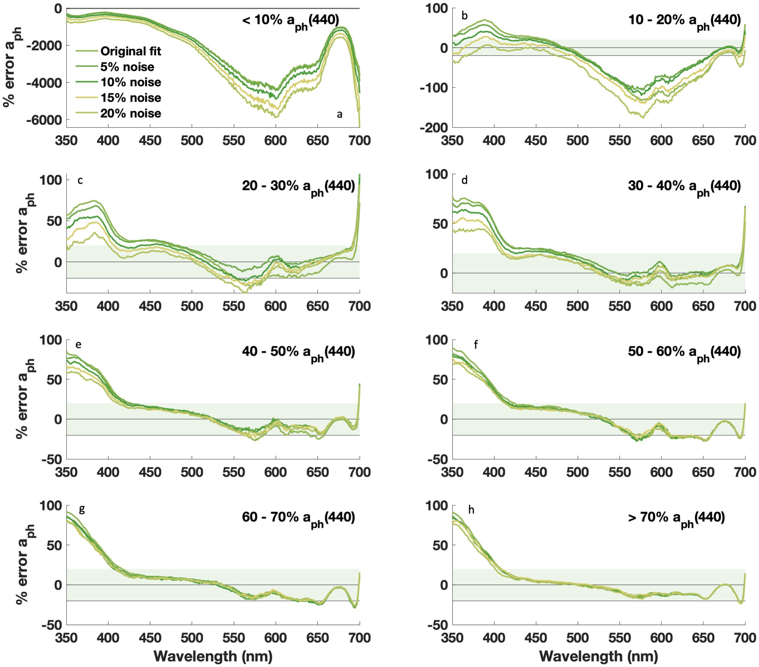
Figure 8. Median percent error vs. wavelength for retrieved a_ph(λ) with DAISEA2 using an exponential relationship for a_dg(λ). Prior to analysis, random noise was added to measured a_nw(λ) in increasing increments of 5%. Data are grouped by % contribution of aph(440), with (a) <10%, (b) 10-20%, (c) 20-30%, (d) 30-40%, (e) 40-50%, (f) 50-60%, (g) 60-70%, and (h) >70%.

Figure 9

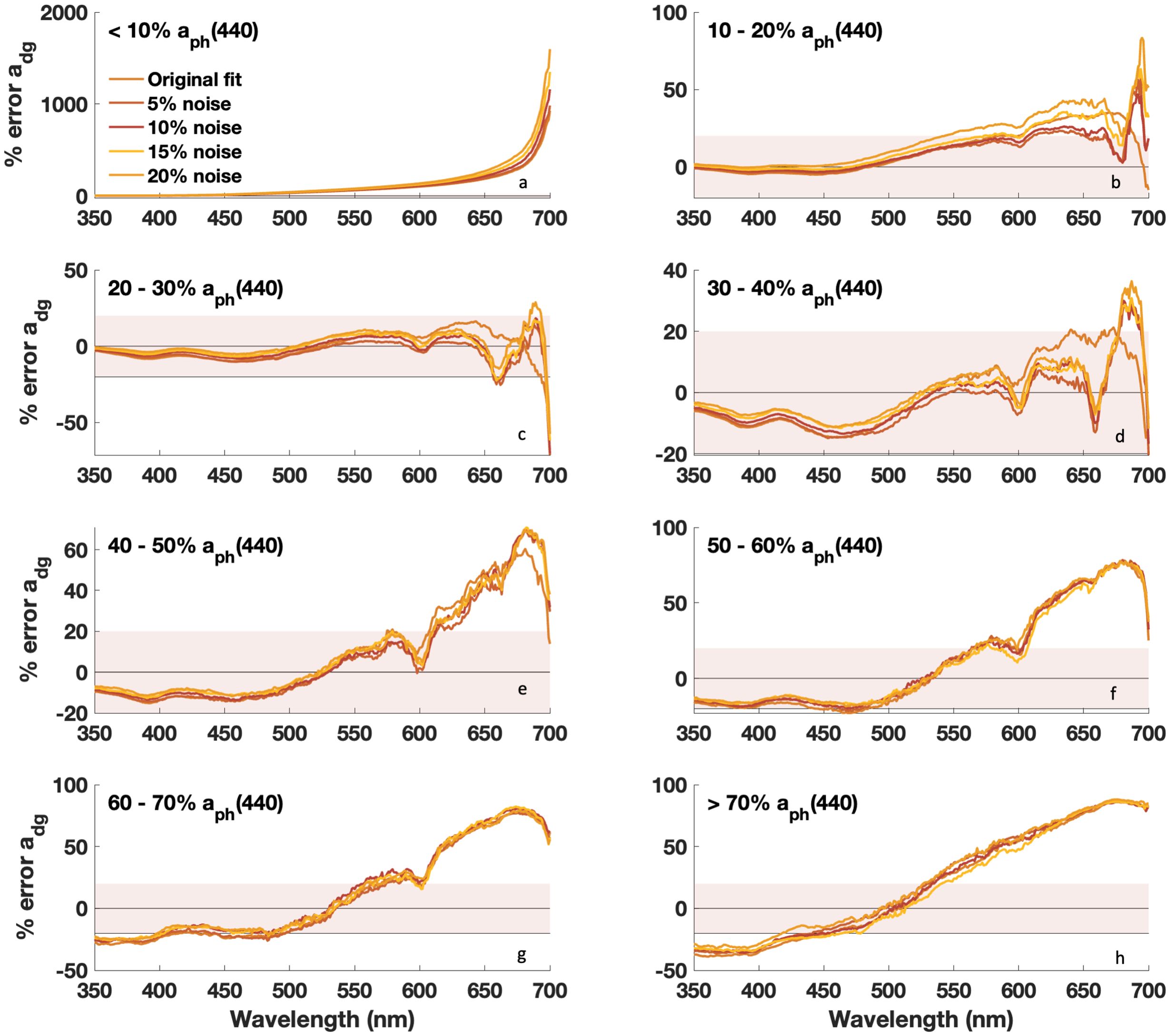
Figure 9. Median percent error vs. wavelength for retrieved a_dg(λ) with DAISEA2 using an exponential relationship for a_dg(λ). Prior to analysis, random noise was added to measured a_nw(λ) in increasing increments of 5%. Data are grouped by % contribution of aph(440), with (a) <10%, (b) 10-20%, (c) 20-30%, (d) 30-40%, (e) 40-50%, (f) 50-60%, (g) 60-70%, and (h) >70%.

4 Discussion

DAISEA2 is intended as a global algorithm, and the assessment of performance here indicates that DAISEA2 should perform well across a variety of optical water types and associated biogeochemical diversity. The algorithm is designed to fit a_dg(λ) and a_ph(λ) free of explicit assumptions, relying on initial empirical estimation of a_dg(440) and a_ph(440) to initialize subsequent spectral fitting and derivative analysis to identify spectral features. Algorithm performance was largely improved relative to the initial algorithm in Grunert et al. (2019), with these improvements predominantly tied to the use of a genetic algorithm to increase the operational search space for ideal model fits. Genetic algorithms enable more successful fitting by allowing “mutants” to supersede initial model parameterizations if the alternative fit provided by the “mutant” is more representative of the underlying spectral features and improves overall model fit and spectral residuals (Houck et al., 1998). Genetic algorithms provide a means for fitting alternative models while still operating within reasonable bounds and, depending on the availability of computational capacity, can operate over reduced or expansive parameter search spaces (Houck et al., 1998; Zhan et al., 2003; Kostadinov et al., 2007). The genetic algorithm is also the best means within DAISEA2 to regionalize the algorithm for more optimal performance, if this is desired, as the parameter space for “mutants” can be restricted to that associated with regional IOPs (e.g., Joshi and D’Sa, 2018; Lewis and Arrigo, 2020). Genetic algorithms are also well suited for hyperspectral approaches that use the observed signal to fit component spectra or features, rather than assuming specific spectral components, as initial estimates are used to populate the search space but, ultimately, alternative fits are offered (see Section 2.2). Ultimately, the distribution in these retrieved components is used to assess uncertainty in retrievals and the extent to which the model converges on similar spectral features as the optimal solution.

Algorithms have historically fallen into two broad classes, top-down and bottom-up approaches, as discussed in the introduction (Mouw et al., 2015). Across these categories, truly hyperspectral algorithms are still limited. The hyperspectral algorithms that do exist often still rely on multispectral techniques, including assumptions about which spectral features are present (Chase et al., 2017; Wang et al., 2016), the use of predefined spectral libraries (Stramski et al., 2019) or inequality constraints (Grunert et al., 2019; Stramski et al., 2019). Alternatively, approaches rely on statistical fitting of a signal, minimizing a physical basis for fitting components and limiting the number of components that can be retrieved, even from hyperspectral sensors (Cael et al., 2023). Producing algorithms that are capable of fitting physical components (e.g., pigments) is often limited by the ability to constrain the signal and still provide a generous search space, producing a global algorithm that can function across systems that display unique IOPs and often generate bias for a given approach. Here, we offer DAISEA2 as a global algorithm that we expect to perform well across a variety of optical gradients and unique biogeochemical conditions, provided effective inversion techniques to provide a_nw(λ) are available (e.g., Loisel et al., 2018; Bi et al., 2023). Our approach in developing DAISEA was to focus on leveraging models that spectrally fit IOPs and informing these models based on pigment locations and reasonable spectral bounds, without providing spectral features for fitting (see Discussion in Grunert et al., 2019). Ultimately, the approach still relies on an initial band ratio to initialize fitting and broad inequality constraints (Equations 4, 5, 10). The empirical relationship still allows strong performance due to this step offering a reasonable, unbiased first guess and the ability for subsequent steps to deviate from this first guess (Supplementary Figure S2). The inequality constraints do support bias in estimates of a_ph(λ), as they limit fitness for fitting of UV pigment features; however, as discussed below, improved guidance is needed to identify spectra with higher magnitudes of a_ph(λ) at UV wavelengths and component features, including absorption due to MAAs. Our inequality constraints are structured on the premise that a_dg(λ) will be responsible for the majority of absorption at UV wavelengths, largely due to a lack of mechanistic understanding of when phytoplankton pigments may contribute to a significant fraction or even the majority of UV absorption, limiting the ability to apply rules to allocate UV absorption to a_ph(λ). We expect that more information on the relationship between visible and UV pigments would help in constraining the magnitude of UV pigments to avoid a_dg(λ) undercutting UV features in a_ph(λ) and typical underestimates of a_ph(λ) by DAISEA2.

We expect that improved knowledge on IOPs, such as through provision of priors within a Bayesian framework, could improve performance as observed with other IOP-based algorithms (e.g., Erickson et al., 2023). This is particularly true in more optically challenging conditions and at UV wavelengths where DAISEA2 remains challenged by singular inequality constraints that do not adequately represent the presence of pigments and elevated a_ph(λ) (Piiparinen et al., 2015); it should be noted that MAA absorption is also present within a_dg(λ), due to the water-soluble nature of these pigments (Pavlov et al., 2014). This further emphasizes the need to expand observations and understanding of aquatic IOPs at UV wavelengths. As with all approaches, it is expected that continued expansion of data collection will improve performance, particularly in undersampled regions and environments that continue to evolve due to anthropogenic, climate, and extreme weather pressures. Efforts, including the current data collection efforts of the PACE Validation Science Team, are expected to improve data availability due to a focus on high coincidence across datasets; while relevant datasets are increasingly available, many of these data were included in development here (e.g., the GLORIA dataset, Lehmann et al., 2023), indicating how data availability and diversity still remain a challenge for effective algorithm development.

Ultimately, DAISEA2 is enabled by the high information content of spectra offered by imaging spectroscopy and hyperspectral spaceborne sensors such as NASA’s PACE OCI or in-situ hyperspectral absorption sensors. Our ability to retrieve component IOPs and relate these features to biogeochemically relevant parameters such as pigment concentrations is dependent on this spectral density and the visibility of individual spectral features (Giese and French, 1955). Here, we employ derivative spectroscopy and Gaussian decomposition to identify spectral wavelengths within a_nw(λ) that are minimally influenced by phytoplankton pigments and to identify pigment locations, consistent with past approaches (Chase et al., 2013; Wang et al., 2016; Chase et al., 2017). We also utilize spectral features within the second derivative to initialize Gaussian decomposition of a_ph(λ), avoiding the need to assume the existence of pigments in contrast to previous approaches, and in line with pigment identification methods (e.g., Bidigare et al., 1989); we do fit ubiquitous pigments when they are not found, but these can still be removed (see Section 2.2). All other algorithms that fit a_ph(λ) using Gaussian components and/or retrieve phytoplankton pigment concentrations from a_ph(λ) rely on predefined pigment characteristics or statistical relationships (Chase et al., 2013, 2017; Liu et al., 2019; Zhang et al., 2021; Teng et al., 2022). Our approach is guided by known pigment locations for classification purposes but ultimately defines a pigment peak based on where the peak is observed within an absorption spectrum using the second derivative, resulting in retrieval of “unclassified” pigment features (Supplementary Figures S6A, B). Three primary principles guided our approach: (1) the presence or absence of pigments is ideally unassumed for a global approach where secondary pigments may not be present, (2) extracted pigments used to characterize individual pigment absorption spectra exhibit shifts in spectral feature location relative to when these pigments are within the cellular matrix (Aguirre-Gomez et al., 2001; Evangelista et al., 2006), and (3) we expect variability in observed peak behavior can be attributed to changes in phytoplankton physiology, community composition, or trait-based approaches to classifying phytoplankton communities (Stuart et al., 1998; Lohrenz et al., 2003; Klais et al., 2017; Weithoff and Beisner, 2019). Here, DAISEA2 actively addresses points 1 and 2 above, while we expect future efforts that begin attributing variability in Gaussian peak locations and features to phytoplankton characteristics, including pigment concentrations and phytoplankton imaging, may be able to leverage this additional information provided by DAISEA2 (Kramer et al., 2024).

DAISEA2 remains challenged in resolving a_ph(λ) at UV wavelengths, with a consistent bias toward underestimating a_ph(λ) at these wavelengths for all spectra regardless of relative contribution of a_ph(440) when using an exponential model to fit a_dg(λ) (Figure 4). Using a hyperbolic model for a_dg(λ) resulted in a positive bias and overestimation of a_ph(λ) at UV wavelengths (Supplementary Figure S8). Across in-situ datasets, our knowledge of UV absorption and phytoplankton pigments is still quite limited. Due to the spectral range of legacy multispectral sensors, many datasets available on NASA’s SeaBASS data archive only collect observations to 400 nm (Werdell and Bailey, 2005). Even when data is collected at wavelengths ≤ 300 nm, methodological errors tend to increase at UV wavelengths, including a lack of guidance on what is considered a “bleached” or depigmented particulate absorption spectra at these wavelengths. Current quality controls are limited to visible wavelengths (e.g., removal of Chl a absorption peaks at blue and red wavelengths; IOCCG Protocol Series, 2018). Many a_ph(λ) data from optically complex inland and coastal waters display increasing absorption at UV wavelengths, providing difficulty in offering rules (e.g., inequality constraints) to separate a_ph(λ) from a_dg(λ) (Figure 10C; Supplementary Figure S10c). Additionally, published Gaussian decomposition approaches do not fit UV pigments outside of Chl a at 382 nm, and spectral absorption is generally limited to either spectra for uncharacterized, community-level features or limited to a single maximum wavelength for specific markers (e.g., Sinha et al., 2007; Chase et al., 2013; Piiparinen et al., 2015; Vale, 2015). Our community ultimately needs to give deeper consideration to UV absorption and pigment features, particularly with the availability of UV wavelengths from remote sensing platforms such as PACE OCI. The information collected by our community, both from spectra as well as data collecting more detailed information on phytoplankton community structure such as Imaging FlowCytobots and other phytoplankton imaging technology, continues to increase our ability to observe unique facets of ecosystem structure and link this to critical global biogeochemical processes from ecosystem productivity to carbon export (Agarwal et al., 2024; Sonnet et al., 2024). With these datasets, the scientific community must continue to expand knowledge on distinct spectral features across UV, visible, and near-infrared wavelengths to maximize the utility of datasets offered by PACE OCI and similar sensors.

Figure 10

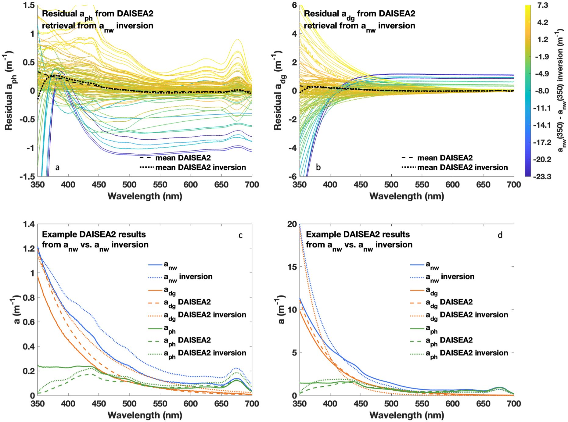
Figure 10. Performance of DAISEA2 retrievals of a_ph(λ) and a_dg(λ) (exponential model) on inversion-retrieved a_nw(λ). DAISEA2’s ability to retrieve accurate a_ph(λ) and a_dg(λ) was dependent on the initial accuracy of inversion-retrieved a_nw(λ) as can be seen in residual spectra (A, B) shaded by residual a_nw(λ) at 350 nm. Examples from two sites (C, D) demonstrate cases where a_ph(λ) can be accurately retrieved despite errors in inversion-retrieved a_nw(λ) and corresponding a_dg(λ).

DAISEA2 ultimately offers improved estimates of pigment concentrations when a_dg(λ) was included in spectral decomposition (Table 2; Figure 7); this was a surprising finding. However, ultimately it indicates that total pigments or the spectral absorption of pigments considered here is underrepresented, both within the literature used to inform the construction of DAISEA (Hoepffner and Sathyendranath, 1993; Chase et al., 2013) and within model implementation. If this were not the case, we would expect a bias in pigment relationships, both within observed and modeled a_ph(λ) variables and HPLC pigments. This further suggests that continued collection of HPLC pigments, improvement on methods for isolating a_ph(λ) in samples from a variety of aquatic systems, and understanding of relationships between pigments and phytoplankton community structure and physiology need to continue to expand to maximize relevance of hyperspectral datasets for evaluating ecosystem functioning and biogeochemical cycles, including providing spectral priors for more explicit fitting of MAAs and other UV-absorbing phytoplankton pigments.

To date, inversion approaches have focused on the delineation of total backscattering [b_b(λ)] and absorption [a(λ)] from R_rs(λ), with subsequent delineation to particulate backscattering [b_bp(λ)] and a_nw(λ) after the removal of backscattering and absorption due to pure water, a known quantity (Pope and Fry, 1997; Zhang et al., 2009; Lee et al., 2002; Werdell et al., 2013). This approach is foundational to IOP retrievals in the community, in part due to less uncertain assumptions tied to the spectral retrieval of b_bp(λ). By nature, these approaches either (1) iteratively separate primary spectral components [b_b(λ) and a(λ)], with a_dg(λ) separated last due to the weakest constraints and highest uncertainty in separating this term into its component absorbing features, a_g(λ) and a_d(λ) (Dong et al., 2013; Stramski et al., 2019) or (2) simultaneously solve for all components by restricting initial starting points and bounds based on previously observed conditions (e.g., Maritorena et al., 2002; Chase et al., 2017). These approaches vary in the degree to which they allow IOP spectra to vary, often requiring spectral priors such as a fixed S_dg (e.g., GIOP; Werdell et al., 2013), spectral libraries or fixed, additive spectral shapes (e.g., Bi et al., 2023), or requiring derived products (e.g., light attenuation coefficient, Loisel et al., 2018). Inversion of R_rs(λ) to a_nw(λ) is expected to spectrally limit derived a_nw(λ) through these assumptions as well as incomplete atmospheric or surface (glint) correction, offering inaccurate starting spectra that will bias retrieved IOPs and corresponding biogeochemical concentrations. We do not expect DAISEA2 to perform well on a_nw(λ) retrieved with fixed spectral shapes or overly rigid spectral priors, but do anticipate that approaches that incorporate a suite of spectra, such as several a_ph(λ) spectra representative of distinct phytoplankton groups, could perform well (e.g., König et al., 2024; Bi et al., 2023). While these approaches still offer a fixed spectra for fitting, the mixing of spectra can enable close approximations of actual underlying a_ph(λ) that offer relatively accurate starting a_nw(λ) for the derivation of component parts using DAISEA2.

To consider the performance of DAISEA2 on inverted a_nw(λ), we used a publicly available dataset collected in the Laurentian Great Lakes in 2024 (https://seabass.gsfc.nasa.gov/experiment/PVST_PRINGLS) and effectively regionalized a publicly available bio-optical package that provides a means of deriving a_nw(λ) from R_rs(λ), with the specifics of data used and inversion parameterization outlined in the Supplementary Material (König et al., 2024; Hondula et al., 2024). In addition to assessing the performance of DAISEA2 on inverted a_nw(λ), this dataset also offered a means of explicitly assessing DAISEA2 performance in optically complex waters. As expected, DAISEA2 performance on inverted a_nw(λ) was primarily controlled by inversion performance (Figure 10; Supplementary Figure S10). The mean residuals for a_ph(λ) and a_dg(λ) were relatively consistent when considering DAISEA2 performance on measured and inverted a_nw(λ); however, when considering performance statistics mirroring those presented in Figure 4 and Supplementary Figure S3, DAISEA2 displayed similar performance on the optically complex dataset from the Laurentian Great Lakes using measured a_nw(λ), but the performance was poorer on inverted a_nw(λ) for most performance metrics (Supplementary Figures S11, S12). One large issue in the inversion is that spectral features in b_bp(λ), consistent with highly absorbing particles, often lead to poor fitting or significant reductions in the magnitude of a_ph(λ). This challenge is evident in a_ph(λ) MAD for inverted a_nw(λ) (Supplementary Figures S11f, S12f) and a_ph(λ) residuals (Figure 10a; Supplementary Figure S10a), which appear as a_ph(λ) spectra. While this early exercise indicates promise for applying DAISEA2 to inverted a_nw(λ), much more work is needed to consider the best approaches for adequately constraining inversion of R_rs(λ), particularly in optically complex waters where b_bp(λ) does not always follow a power law model. In particular, the performance of DAISEA2 against other state-of-the-art hyperspectral inversion approaches is needed to more fully assess the strengths and weaknesses of DAISEA2 relative to other approaches and the potential performance of DAISEA2 with PACE data. This will be particularly informative in understanding how various assumptions used across inversion approaches influence resulting retrieved spectra and should be the focus of future work. It is also important to note that our consideration of DAISEA2 performance on inverted a_nw(λ), as well as our analysis of DAISEA2 performance on artificially noisy spectra, does not account for spectral artifacts or wavelength-dependent bias associated with atmospheric correction of satellite data. These impacts are likely to be significant, particularly at UV wavelengths where DAISEA2 is already challenged and require future investigation to fully assess the ability of DAISEA2 to accurately and reliably retrieve IOPs from satellite datasets such as those offered by PACE.

Finally, separating a_dg(λ) into a_g(λ) and a_d(λ) was a stated goal of future developments of DAISEA (Grunert et al., 2019). However, our view is that future modifications to DAISEA to delineate a_g(λ) and a_d(λ) will require additional inputs of independent information that specifically acknowledge relative contributions of each to offer a physical basis for separation with limited empiricism (e.g., Bisson et al., 2023). Within the current framework of the algorithm, separation of these two terms will increase uncertainty across all parameters, limiting our ability to estimate a_ph(λ) and corresponding pigments. We view lidar, and potentially polarimetry, as two data sources that could provide potential avenues for informed separation (Jamet et al., 2019; Dionisi et al., 2024).

5 Conclusion

The primary goal of DAISEA2 was to decompose hyperspectral a_nw(λ) into a_dg(λ) and a_ph(λ) free of explicit assumptions, while integrating a framework that provides uncertainty estimates for all retrieved parameters, including future efforts focused on estimating phytoplankton pigment concentrations from retrieved Gaussian components. DAISEA2 shows strong capability to accurately retrieve a_dg(λ) and a_ph(λ) across a variety of water types, indicating global applicability within aquatic systems represented by the diversity of conditions considered here. This performance was reinforced on an independent dataset collected in the optically complex Laurentian Great Lakes. Based on the flexibility of the algorithm and its ability to actively retrieve and parameterize spectral features, along with the ability to expand the search space from initial parameterizations through a genetic algorithm, we expect the algorithm to perform well even in systems that differ optically from the datasets used to develop the algorithm here. This was supported by consistent performance between the development and validation datasets used in Grunert et al. (2019) and similar performance on an independent dataset from the optically complex waters of the Laurentian Great Lakes. DAISEA2 exhibits a negative bias in retrieval of a_ph(λ) at UV wavelengths, in part because the algorithm is biased toward assuming that UV absorption is due to a_dg(λ), as we lack spectral indicators to attribute UV absorption to a_ph(λ). When paired with known issues with atmospheric correction of PACE data at UV wavelengths, these challenges are likely to increase with inverted a_nw(λ) from satellite sensors. These weaknesses highlight a need for future work to improve constraints and accurate pigment retrievals at UV wavelengths and evaluate the performance of DAISEA2 on satellite datasets. Additionally, our community should continue to expand understanding of spectral features at UV wavelengths and provide pathways for partitioning absorption to component IOPs, including offering spectral priors for MAAs and other UV-absorbing pigments in hyperspectral algorithms.

The modest to strong relationships between DAISEA2-retrieved Gaussian parameters and HPLC-measured phytoplankton pigment concentrations indicate that DAISEA2 will provide estimates of phytoplankton pigment concentration with reasonable accuracy and uncertainty, outside of demonstrated bias at UV wavelengths. Algorithm performance is relatively robust to spectral resolution and simulated random noise, and DAISEA2 performed well on inverted a_nw(λ) when the inversion itself was accurate. However, performance significantly deteriorated with decreasing inversion success, a limitation that is likely to be exacerbated when applied to satellite datasets with spectral biases introduced from atmospheric correction. Future work to continue improving inversion approaches that maximize spectral variability while still adequately constraining the inversion process is needed, as has been acknowledged in the literature and through ongoing activities across the ocean color community. Additionally, future work should assess how atmospheric correction and introduced spectral artifacts impact DAISEA2 performance on inverted a_nw(λ) from satellite datasets. Key to any improvements for DAISEA2 and other hyperspectral algorithms is the continuing collection of fully coincident, hyperspectral datasets by the community to further evaluate and improve algorithm performance. Finally, DAISEA2 is still dependent on some tools designed for spectrally limited datasets, such as band ratios and inequality constraints. We view these steps as limiting to overall performance, which highlights the need for the community to continue focusing on the development of unique tools that leverage the spectral density of information offered by sensors such as PACE OCI.

Data availability statement

Publicly available datasets were analyzed in this study. This data can be found here: https://seabass.gsfc.nasa.gov/.

Author contributions

BG: Conceptualization, Data curation, Formal Analysis, Funding acquisition, Investigation, Methodology, Project administration, Resources, Software, Supervision, Validation, Visualization, Writing – original draft, Writing – review & editing. AC: Conceptualization, Data curation, Formal Analysis, Investigation, Methodology, Software, Validation, Visualization, Writing – original draft, Writing – review & editing. CM: Conceptualization, Funding acquisition, Methodology, Writing – review & editing.

Funding

The author(s) declare that financial support was received for the research and/or publication of this article. The research completed here was supported by NASA’s New Investigator Program (80NSSC22K0341), Remote Sensing of Water Quality program (80NSSC22K1298), and PACE Mission Validation (80NSSC24K0717).

Acknowledgments

We would like to thank members of the Carbon & (H₂)Optics Lab at Cleveland State University, in particular Emily Hyland and Kendra Herweck for supporting use of the bio-optics Python package, and the Aquatic Optics & Remote Sensing Lab at the University of Rhode Island for helpful comments and feedback throughout algorithm development and refinement. Thank you to all data providers and NASA’s SeaBASS data archive team for making this research possible. We would also like to thank Kendra Herweck, the editor, and reviewers for feedback critical to the final version of this article.

Conflict of interest

The authors declare that the research was conducted in the absence of any commercial or financial relationships that could be construed as a potential conflict of interest.

Generative AI statement

The author(s) declare that no Generative AI was used in the creation of this manuscript.

Publisher’s note

All claims expressed in this article are solely those of the authors and do not necessarily represent those of their affiliated organizations, or those of the publisher, the editors and the reviewers. Any product that may be evaluated in this article, or claim that may be made by its manufacturer, is not guaranteed or endorsed by the publisher.

Supplementary material

The Supplementary Material for this article can be found online at: https://www.frontiersin.org/articles/10.3389/fmars.2025.1549312/full#supplementary-material

References

Agarwal V., Sonnet V., Inomura K., Ciochetto A. B., and Mouw C. B. (2024). Image-derived indicators of phytoplankton community responses to Pseudo-nitzschia blooms. Harmful Algae 138, 102702. doi: 10.1016/j.hal.2024.102702

PubMed Abstract | Crossref Full Text | Google Scholar

Aguirre-Gomez R., Weeks A. R., and Boxall S. R. (2001). The identification of phytoplankton pigments from absorption spectra. Int. J. Remote Sens. 22, 315–338. doi: 10.1080/014311601449952

Crossref Full Text | Google Scholar

Albert A. and Gege P. (2006). Inversion of irradiance and remote sensing reflectance in shallow water between 400 and 800 nm for calculations of water and bottom properties. Appl. Optics 45, 2331–2343. doi: 10.1364/AO.45.002331

PubMed Abstract | Crossref Full Text | Google Scholar

Albert A. and Mobley C. (2003). An analytical model for subsurface irradiance and remote sensing reflectance in deep and shallow case-2 waters. Optics Express 11, 2873–2890. doi: 10.1364/OE.11.002873

PubMed Abstract | Crossref Full Text | Google Scholar

Anderson D. M., Fachon E., Pickart R. S., Lin P., Fischer A. D., Richlen M. L., et al. (2021). Evidence for massive and recurrent toxic blooms of Alexandrium catenella in the Alaskan Arctic. Proc. Natl. Acad. Sci. 118, e2107387118. doi: 10.1073/pnas.2107387118

PubMed Abstract | Crossref Full Text | Google Scholar

Behrenfeld M. J. and Milligan A. J. (2013). Photophysiological expressions of iron stress in phytoplankton. Annu. Rev. marine Sci. 5, 217–246. doi: 10.1146/annurev-marine-121211-172356

PubMed Abstract | Crossref Full Text | Google Scholar

Bi S., Hieronymi M., and Röttgers R. (2023). Bio-geo-optical modelling of natural waters. Front. Marine Sci. 10, 1196352. doi: 10.3389/fmars.2023.1196352

Crossref Full Text | Google Scholar

Bidigare R. R., Morrow J. H., and Kiefer D. A. (1989). Derivative analysis of spectral absorption by photosynthetic pigments in the western Sargasso Sea. J. Mar. Res. 47 (2). doi: 10.1357/002224089785076325

Crossref Full Text | Google Scholar

Bisson K. M., Werdell P. J., Chase A. P., Kramer S. J., Cael B. B., Boss E., et al. (2023). Informing ocean color inversion products by seeding with ancillary observations. Optics Express 31, 40557–40572. doi: 10.1364/OE.503496

PubMed Abstract | Crossref Full Text | Google Scholar

Blanchet C. C., Arzel C., Davranche A., Kahilainen K. K., Secondi J., Taipale S., et al. (2022). Ecology and extent of freshwater browning-What we know and what should be studied next in the context of global change. Sci. Total Environ. 812, 1524205. doi: 10.1016/j.scitotenv.2021.152420

PubMed Abstract | Crossref Full Text | Google Scholar

Bricaud A., Claustre H., Ras J., and Oubelkheir K. (2004). Natural variability of phytoplanktonic absorption in oceanic waters: Influence of the size structure of algal populations. J. Geophysical Research: Oceans 109. doi: 10.1029/2004JC002419

Crossref Full Text | Google Scholar

Cael B. B., Bisson K., Boss E., and Erickson Z. K. (2023). How many independent quantities can be extracted from ocean color? Limnology Oceanography Lett. 8, 603–610. doi: 10.1002/lol2.10319

Crossref Full Text | Google Scholar

Cael B. B. and Boss E. (2017). Simplified model of spectral absorption by non-algal particles and dissolved organic materials in aquatic environments. Optics Express 25, 25486–25491. doi: 10.1364/OE.25.025486

PubMed Abstract | Crossref Full Text | Google Scholar

Cao F. and Tzortziou M. (2024). Impacts of hydrology and extreme events on dissolved organic carbon dynamics in a heavily urbanized estuary and its major tributaries: a view from space. J. Geophysical Res. 129, e2023JG007767. doi: 10.1029/2023JG007767

Crossref Full Text | Google Scholar

Carreto J. I., Carignan M. O., Montoya N. G., Cozzolino E., and Akselman R. (2018). Mycosporine-like amino acids and xanthophyll-cycle pigments favour a massive spring bloom development of the dinoflagellate Prorocentrum minimum in Grande Bay (Argentina), an ozone hole affected area. J. Marine Syst. 178, 15–28. doi: 10.1016/j.jmarsys.2017.10.004

Crossref Full Text | Google Scholar

Cetinić I., Rousseaux C. S., Carroll I. T., Chase A. P., Kramer S. J., P. Werdell J., et al. (2024). Phytoplankton composition from sPACE: Requirements, opportunities, and challenges. Remote Sens. Environ. 302, 1139645. doi: 10.1016/j.rse.2023.113964

Crossref Full Text | Google Scholar

Chase A. P., Boss E., Cetinić I., and Slade W. (2017). Estimation of phytoplankton accessory pigments from hyperspectral reflectance spectra: toward a global algorithm. J. Geophysical Res. 122, 9725–9743. doi: 10.1002/2017JC012859

Crossref Full Text | Google Scholar

Chase A., Boss E., Zaneveld R., Bricaud A., Claustre H., Ras J., et al. (2013). Decomposition of in situ particulate absorption spectra. Methods Oceanography 7, 110–124. doi: 10.1016/j.mio.2014.02.002

Crossref Full Text | Google Scholar

Cooney E. M., McKinney P., Sterner R., Small G. E., and Minor E. C. (2018). Tale of two storms: Impact of extreme rain events on the biogeochemistry of Lake Superior. J. Geophysical Res. 123, 1719–1731. doi: 10.1029/2017JG004216

PubMed Abstract | Crossref Full Text | Google Scholar

D’Sa E. J., Tzortziou M., and Liu B. (2023). Extreme events and impacts on organic carbon cycles from ocean color remote sensing: Review with case study, challenges, and future directions. Earth-Science Rev. 243, 104503. doi: 10.1016/j.earscirev.2023.104503

Crossref Full Text | Google Scholar

Descy J. P., Sarmento H., and Higgins H. W. (2009). Variability of phytoplankton pigment ratios across aquatic environments. Eur. J. Phycology 44, 319–330. doi: 10.1080/09670260802618942

Crossref Full Text | Google Scholar

Dickey T., Lewis M., and Chang G. (2006). Optical oceanography: recent advances and future directions using global remote sensing and in situ observations. Rev. geophysics 44. doi: 10.1029/2003RG000148

Crossref Full Text | Google Scholar

Dierssen H. M., Ackleson S. G., Joyce K. E., Hestir E. L., Castagna A., Lavender S., et al. (2021). Living up to the hype of hyperspectral aquatic remote sensing: science, resources and outlook. Front. Environ. Sci. 9, 649528. doi: 10.3389/fenvs.2021.649528

Crossref Full Text | Google Scholar

Dionisi D., Bucci S., Cesarini C., Colella S., D’Alimonte D., Di Ciolo L., et al. (2024). Exploring the potential of Aeolus lidar mission for ocean color applications. Remote Sens. Environ. 313, 114341. doi: 10.1016/j.rse.2024.114341

Crossref Full Text | Google Scholar

Dong Q., Shang S., and Lee Z. (2013). An algorithm to retrieve absorption coefficient of chromophoric dissolved organic matter from ocean color. Remote Sens. Environ. 128, 259–267. doi: 10.1016/j.rse.2012.10.013

Crossref Full Text | Google Scholar

Eisner L. B. and Cowles T. J. (2005). Spatial variations in phytoplankton pigment ratios, optical properties, and environmental gradients in Oregon coast surface waters. J. Geophysical Res. 110. doi: 10.1029/2004JC002614

Crossref Full Text | Google Scholar

Erickson Z. K., McKinna L., Werdell P. J., and Cetinić I. (2023). Bayesian approach to a generalized inherent optical property model. Optics Express 31, 22790–22801. doi: 10.1364/OE.486581

PubMed Abstract | Crossref Full Text | Google Scholar

Evangelista V., Frassanito A. M., Passarelli V., Barsanti L., and Gualtieri P. (2006). Microspectroscopy of the photosynthetic compartment of algae. Photochemistry photobiology 82, 1039–1046. doi: 10.1562/2006-01-11-RA-772

PubMed Abstract | Crossref Full Text | Google Scholar

Fogarty M. J., Rosenberg A. A., Cooper A. B., Dickey-Collas M., Fulton E. A., Gutiérrez N. L., et al. (2016). Fishery production potential of large marine ecosystems: A prototype analysis. Environ. Dev. 17, 211–2195. doi: 10.1016/j.envdev.2016.02.001

Crossref Full Text | Google Scholar

Giese A. T. and French C. S. (1955). The analysis of overlapping spectral absorption bands by derivative spectrophotometry. Appl. Spectrosc. 9, 78–96. doi: 10.1366/000370255774634089

Crossref Full Text | Google Scholar

Grunert B. K., Mouw C. B., and Ciochetto A. B. (2018). Characterizing CDOM spectral variability across diverse regions and spectral ranges. Global Biogeochemical Cycles 32, 57–77. doi: 10.1002/2017GB005756

Crossref Full Text | Google Scholar

Grunert B. K., Mouw C. B., and Ciochetto A. B. (2019). Deriving inherent optical properties from decomposition of hyperspectral non-water absorption. Remote Sens. Environ. 225, 193–206. doi: 10.1016/j.rse.2019.03.004

Crossref Full Text | Google Scholar

Häder D. P. and Barnes P. W. (2019). Comparing the impacts of climate change on the responses and linkages between terrestrial and aquatic ecosystems. Sci. Total Environ. 682, 239–246. doi: 10.1016/j.scitotenv.2019.05.024

PubMed Abstract | Crossref Full Text | Google Scholar

Helms J. R., Stubbins A., Ritchie J. D., Minor E. C., Kieber D. J., and Mopper K. (2008). Absorption spectral slopes and slope ratios as indicators of molecular weight, source, and photobleaching of chromophoric dissolved organic matter. Limnology oceanography 53, 955–969. doi: 10.4319/lo.2008.53.3.0955

Crossref Full Text | Google Scholar

Hoepffner N. and Sathyendranath S. (1991). Effect of pigment composition on absorption properties of phytoplankton. Mar. Ecol. Prog. Ser. 73, 11–23. doi: 10.3354/meps073011

Crossref Full Text | Google Scholar

Hoepffner N. and Sathyendranath S. (1993). Determination of the major groups of phytoplankton pigments from the absorption spectra of total particulate matter. J. Geophysical Res. 98, 22789–22803. doi: 10.1029/93JC01273

Crossref Full Text | Google Scholar

Holland J. (1975). Adaptation in Natural and Artificial Systems (Ann Arbor: The University of Michigan Press).

Google Scholar

Hondula K. L., König M., Grunert B. K., Vaughn N. R., Martin R. E., Dai J., et al. (2024). Mapping water quality in nearshore reef environments using airborne imaging spectroscopy. Remote Sens. 16, 1845. doi: 10.3390/rs16111845

Crossref Full Text | Google Scholar

Houck C., Joines J., and Kay M. (1998). A Genetic Algorithm for Function Optimization: A Matlab Implementation NCSUIE-TR-95-09. (Raleigh, NC, USA: North Carolina State University), 22. Available online at: http://www.ie.ncsu.edu/mirage/GAToolBox/gaot/.

Google Scholar

IOCCG Protocol Series (2018). “Inherent optical property measurements and protocols: absorption coefficient,” in IOCCG Ocean Optics and Biogeochemistry Protocols for Satellite Ocean Colour Sensor Validation, Volume 1.0. Eds. Neeley A. R. and Mannino A. (IOCCG, Dartmouth, NS, Canada). doi: 10.25607/OBP-119

Crossref Full Text | Google Scholar

Jacinavicius F. R., Geraldes V., Crnkovic C. M., Delbaje E., Fiore M. F., and Pinto E. (2021). Effect of ultraviolet radiation on the metabolomic profiles of potentially toxic cyanobacteria. FEMS Microbiol. Ecol. 97, fiaa243. doi: 10.1093/femsec/fiaa243

PubMed Abstract | Crossref Full Text | Google Scholar

Jamet C., Ibrahim A., Ahmad Z., Angelini F., Babin M., Behrenfeld M. J., et al. (2019). Going beyond standard ocean color observations: lidar and polarimetry. Front. Marine Sci. 6, 2515. doi: 10.3389/fmars.2019.00251

Crossref Full Text | Google Scholar

Johnson L., Siegel D. A., Thompson A. F., Fields E., Erickson Z. K., Cetinic I., et al. (2024). Assessment of oceanographic conditions during the North Atlantic EXport processes in the ocean from RemoTe sensing (EXPORTS) field campaign. Prog. Oceanography 220, 1031705. doi: 10.1016/j.pocean.2023.103170

Crossref Full Text | Google Scholar

Jorge D. S. F., Loisel H., Jamet C., Dessailly D., Demaria J., Bricaud A., et al. (2021). A three-step semi analytical algorithm (3SAA) for estimating inherent optical properties over oceanic, coastal, and inland waters from remote sensing reflectance. Remote Sens. Environ. 263, 1125375. doi: 10.1016/j.rse.2021.112537

Crossref Full Text | Google Scholar

Joshi I. D. and D’Sa E. J. (2018). An estuarine-tuned quasi-analytical algorithm (QAA-V): assessment and application to satellite estimates of SPM in Galveston Bay following Hurricane Harvey. Biogeosciences 15, 4065–4086. doi: 10.5194/bg-15-4065-2018

Crossref Full Text | Google Scholar

Joshi I. D., Stramski D., Reynolds R. A., and Robinson D. H. (2023). Performance assessment and validation of ocean color sensor-specific algorithms for estimating the concentration of particulate organic carbon in oceanic surface waters from satellite observations. Remote Sens. Environ. 286, 113417. doi: 10.1016/j.rse.2022.113417

Crossref Full Text | Google Scholar

Klais R., Norros V., Lehtinen S., Tamminen T., and Olli K. (2017). Community assembly and drivers of phytoplankton functional structure. Funct. Ecol. 31, 760–767. doi: 10.1111/fec.2017.31.issue-3

Crossref Full Text | Google Scholar

König M., Hondula K., Noel P., Nick V., and Asner G. (2024). Cmlandocean/bio_optics: V0.0.2 (Zenodo). doi: 10.5281/zenodo.14187746

Crossref Full Text | Google Scholar

Kostadinov T. S., Diegel D. A., Maritorena S., and Guillocheau N. (2007). Ocean color observations and modeling for an optically complex site: Santa Barbara Channel, California, USA. JGR 112, C07011. doi: 10.1029/2006JC003526

Crossref Full Text | Google Scholar

Kramer S. J., Bolaños L. M., Catlett D., Chase A. P., Behrenfeld M. J., Boss M. S., et al. (2024). Toward a synthesis of phytoplankton community composition methods for global-scale application. Limnology Oceanography 22, 217–240. doi: 10.1002/lom3.10602

Crossref Full Text | Google Scholar

Lee Z. and Carder K. L. (2004). Absorption spectrum of phytoplankton pigments derived from hyperspectral remote-sensing reflectance. Remote Sens. Environ. 89, 361–368. doi: 10.1016/j.rse.2003.10.013

Crossref Full Text | Google Scholar

Lee Z., Carder K. L., and Arnone R. A. (2002). Deriving inherent optical properties from water color: a multiband quasi-analytical algorithm for optically deep waters. Appl. optics 41, 5755–5772. doi: 10.1364/AO.41.005755

PubMed Abstract | Crossref Full Text | Google Scholar

Lehmann M. K., Gurlin D., Pahlevan N., Alikas K., Conroy T., Anstee J., et al. (2023). GLORIA-A globally representative hyperspectral in situ dataset for optical sensing of water quality. Sci. Data 10, 100. doi: 10.1038/s41597-023-01973-y

PubMed Abstract | Crossref Full Text | Google Scholar

Lewis K. M. and Arrigo K. R. (2020). Ocean color algorithms for estimating chlorophyll a, CDOM absorption, and particle backscattering in the Arctic Ocean. J. Geophysical Res. 125, e2019JC015706. doi: 10.1029/2019JC015706

Crossref Full Text | Google Scholar

Liu Y., Boss E., Chase A., Xi H., Zhang X., Röttgers R., et al. (2019). Retrieval of phytoplankton pigments from underway spectrophotometry in the Fram Strait. Remote Sens. 11, 318. doi: 10.3390/rs11030318

Crossref Full Text | Google Scholar

Liu B., D’Sa E. J., Messina F., Baustian M. M., Maiti K., Rivera-Monroy V. H., et al. (2023). Dissolved organic carbon dynamics and fluxes in Mississippi-Atchafalaya deltaic system impacted by an extreme flood event and hurricanes: a multi-satellite approach using Sentinel-2/3 and Landsat-8/9 data. Front. Marine Sci. 10, 1159367. doi: 10.3389/fmars.2023.1159367

Crossref Full Text | Google Scholar

Lohrenz S. E., Weidemann A. D., and Tuel M. (2003). Phytoplankton spectral absorption as influenced by community size structure and pigment composition. J. Plankton Res. 25, 35–61. doi: 10.1093/plankt/25.1.35

Crossref Full Text | Google Scholar

Loisel H., Jorge D. S. F., Reynolds R. A., and Stramski D. (2023). A synthetic optical database generated by radiative transfer simulations in support of studies in ocean optics and optical remote sensing of the global ocean. Earth System Sci. Data 15, 3711–3731. doi: 10.5194/essd-15-3711-2023

Crossref Full Text | Google Scholar

Loisel H., Stramski D., Dessailly D., Jamet C., Li L., and Reynolds R. A. (2018). An inverse model for estimating the optical absorption and backscattering coefficients of seawater from remote-sensing reflectance over a broad range of oceanic and coastal marine environments. J. Geophysical Res. 123, 2141–2171. doi: 10.1002/2017JC013632

Crossref Full Text | Google Scholar

Lomas M. W., Neeley A. R., Vandermeulen R., Mannino A., Thomas C., Novak M. G., et al. (2024). Phytoplankton optical fingerprint libraries for development of phytoplankton ocean color satellite products. Sci. Data 11, 168. doi: 10.1038/s41597-024-03001-z

PubMed Abstract | Crossref Full Text | Google Scholar

Lombard F., Boss E., Waite A. M., Vogt M., Uitz J., Stemmann L., et al. (2019). Globally consistent quantitative observations of planktonic ecosystems. Front. Marine Sci. 6, 1965. doi: 10.3389/fmars.2019.00196

Crossref Full Text | Google Scholar

Maritorena S., Siegel D. A., and Peterson A. R. (2002). Optimization of a semianalytical ocean color model for global-scale applications. Appl. optics 41, 2705–2714. doi: 10.1364/AO.41.002705

PubMed Abstract | Crossref Full Text | Google Scholar

McKibben S. M., Uz S. S., and Palacios S. L. (2024). Testing a hyperspectral, bio-optical approach to identification of phytoplankton community composition in the Chesapeake Bay estuary. Earth Space Sci. 11, e2023EA003244. doi: 10.1029/2023EA003244

Crossref Full Text | Google Scholar

Mouw C. B., Barnett A., McKinley G. A., Gloege L., and Pilcher D. (2016). Phytoplankton size impact on export flux in the global ocean. Global Biogeochemical Cycles 30, 1542–1562. doi: 10.1002/2015GB005355

Crossref Full Text | Google Scholar

Mouw C. B., Ciochetto A. B., and Yoder J. A. (2019). A satellite assessment of environmental controls of phytoplankton community size structure. Global Biogeochemical Cycles 33, 540–558. doi: 10.1029/2018GB006118

Crossref Full Text | Google Scholar

Mouw C. B., Greb S., Aurin D., DiGiacomo P. M., Lee Z., Twardowski M., et al. (2015). Aquatic color radiometry remote sensing of coastal and inland waters: Challenges and recommendations for future satellite missions. Remote Sens. Environ. 160, 15–305. doi: 10.1016/j.rse.2015.02.001

Crossref Full Text | Google Scholar

Osburn C. L., Rudolph J. C., Paerl H. W., Hounshell A. G., and Van Dam B. R. (2019). Lingering carbon cycle effects of Hurricane Matthew in North Carolina’s coastal waters. Geophysical Res. Lett. 46, 2654–2661. doi: 10.1029/2019GL082014

Crossref Full Text | Google Scholar

Paerl H. W., Hall N. S., Hounshell A. G., Luettich R. A. Jr., Rossignol K. L., Osburn C. L., et al. (2019). Recent increase in catastrophic tropical cyclone flooding in coastal North Carolina, USA: Long-term observations suggest a regime shift. Sci. Rep. 9, 10620. doi: 10.1038/s41598-019-46928-9

PubMed Abstract | Crossref Full Text | Google Scholar

Pavlov A. K., Silyakova A., Granskog M. A., Bellerby R. G. J., Engel A., Schulz K. G., et al. (2014). Marine CDOM accumulation during a coastal Arctic mesocosm experiment: No response to elevated pCO2 levels. J. Geophysical Res. 119, 1216–1230. doi: 10.1002/2013JG002587

Crossref Full Text | Google Scholar

Piiparinen J., Enberg S., Rintala J. M., Sommaruga R., Majaneva M., Autio R., et al. (2015). The contribution of mycosporine-like amino acids, chromophoric dissolved organic matter and particles to the UV protection of sea-ice organisms in the Baltic Sea. Photochemical Photobiological Sci. 14, 1025–1038. doi: 10.1039/c4pp00342j

PubMed Abstract | Crossref Full Text | Google Scholar

Pope R. M. and Fry E. S. (1997). Absorption spectrum (380–700 nm) of pure water. II. Integrating cavity measurements. Appl. optics 36, 8710–8723. doi: 10.1364/AO.36.008710

PubMed Abstract | Crossref Full Text | Google Scholar

Reinl K. L., Sterner R. W., Lafrancois B. M., and Brovold S. (2020). Fluvial seeding of cyanobacterial blooms in oligotrophic Lake Superior. Harmful Algae 100, 101941. doi: 10.1016/j.hal.2020.101941

PubMed Abstract | Crossref Full Text | Google Scholar

Seegers B. N., Stumpf R. P., Schaeffer B. A., Loftin K. A., and Werdell P. J. (2018). Performance metrics for the assessment of satellite data products: an ocean color case study. Optics express 26, 7404–7422. doi: 10.1364/OE.26.007404

PubMed Abstract | Crossref Full Text | Google Scholar

Sinha R. P., Singh S. P., and Häder D. P. (2007). Database on mycosporines and mycosporine-like amino acids (MAAs) in fungi, cyanobacteria, macroalgae, phytoplankton and animals. J. Photochemistry Photobiology B 89, 29–35. doi: 10.1016/j.jphotobiol.2007.07.006

PubMed Abstract | Crossref Full Text | Google Scholar

Sonnet V., Mouw C. B., Ciochetto A. B., and Carney-Almeida J. (2024). Hit or miss? Impact of time series resolution on resolving phytoplankton dynamics at hourly, weekly, and satellite remote sensing frequencies. Limnology Oceanography 22, 254–267. doi: 10.1002/lom3.10604

Crossref Full Text | Google Scholar

Sterner R. W., Reinl K. L., Lafrancois B. M., Brovold S., and Miller T. R. (2020). A first assessment of cyanobacterial blooms in oligotrophic Lake Superior. Limnology Oceanography 65, 2984–2998. doi: 10.1002/lno.v65.12

Crossref Full Text | Google Scholar

Stramski D., Li L., and Reynolds R. A. (2019). Model for separating the contributions of non-algal particles and colored dissolved organic matter to light absorption by seawater. Appl. Optics 58, 3790–3806. doi: 10.1364/AO.58.003790

PubMed Abstract | Crossref Full Text | Google Scholar

Stuart V., Sathyendranath S., Platt T., Maass H., and Irwin B. D. (1998). Pigments and species composition of natural phytoplankton populations: effect on the absorption spectra. J. Plankton Res. 20, 187–217. doi: 10.1093/plankt/20.2.187

Crossref Full Text | Google Scholar

Teng J., Zhang T., Sun K., and Gao H. (2022). Retrieving pigment concentrations based on hyperspectral measurements of the phytoplankton absorption coefficient in global oceans. Remote Sens. 14, 3516. doi: 10.3390/rs14153516

Crossref Full Text | Google Scholar

Tsai F. and Philpot W. (1998). Derivative analysis of hyperspectral data. Remote Sens. Environ. 66, 41–51. doi: 10.1016/S0034-4257(98)00032-7

Crossref Full Text | Google Scholar

Turak E., Harrison I., Dudgeon D., Abell R., Bush A., Darwall W., et al. (2017). Essential biodiversity variables for measuring change in global freshwater biodiversity. Biol. Conserv. 213, 272–2795. doi: 10.1016/j.biocon.2016.09.005

Crossref Full Text | Google Scholar

Twardowski M. S., Boss E., Sullivan J. M., and Donaghay P. L. (2004). Modeling the spectral shape of absorption by chromophoric dissolved organic matter. Marine Chem. 89, 69–88. doi: 10.1016/j.marchem.2004.02.008

Crossref Full Text | Google Scholar

Vale P. (2015). Effects of light quality and nutrient availability on accumulation of mycosporine-like amino acids in Gymnodinium catenatum (Dinophycea). J. Photochemistry Photobiology B 143, 20–29. doi: 10.1016/j.jphotobiol.2014.12.016

PubMed Abstract | Crossref Full Text | Google Scholar

Wang M., Hu C., Barnes B. B., Mitchum G., Lapointe B., and Montoya J. P. (2019). The great Atlantic sargassum belt. Science 365, 83–87. doi: 10.1126/science.aaw7912

PubMed Abstract | Crossref Full Text | Google Scholar

Wang G., Lee Z., Mishra D. R., and Ma R. (2016). Retrieving absorption coefficients of multiple phytoplankton pigments from hyperspectral remote sensing reflectance measured over cyanobacteria bloom waters. Limnology Oceanography 14, 432–447. doi: 10.1002/lom3.10102

Crossref Full Text | Google Scholar

Wang G., Lee Z., and Mouw C. (2017). Multi-spectral remote sensing of phytoplankton pigment absorption properties in cyanobacteria bloom waters: A regional example in the western basin of Lake Erie. Remote Sens. 9, 1309. doi: 10.3390/rs9121309

Crossref Full Text | Google Scholar

Weithoff G. and Beisner B. E. (2019). Measures and approaches in trait-based phytoplankton community ecology–from freshwater to marine ecosystems. Front. Marine Sci. 6, 40. doi: 10.3389/fmars.2019.00040

Crossref Full Text | Google Scholar

Werdell P. J. and Bailey S. W. (2005). An improved in-situ bio-optical data set for ocean color algorithm development and satellite data product validation. Remote Sens. Environ. 98, 122–140. doi: 10.1016/j.rse.2005.07.001

Crossref Full Text | Google Scholar

Werdell P. J., Franz B. A., Bailey S. W., Feldman G. C., Boss E., Brando V. E., et al. (2013). Generalized ocean color inversion model for retrieving marine inherent optical properties. Appl. optics 52, 2019–2037. doi: 10.1364/AO.52.002019

PubMed Abstract | Crossref Full Text | Google Scholar

Wetzels R. and Wagenmakers E. J. (2012). A default Bayesian hypothesis test for correlations and partial correlations. Psychonomic Bull. Rev. 19, 1057–1064. doi: 10.3758/s13423-012-0295-x

PubMed Abstract | Crossref Full Text | Google Scholar

Zhan H., Lee Z., Shi P., Chen C., and Carder K. L. (2003). Retrieval of water optical properties for optically deep waters using genetic algorithms. IEEE Trans. Geosci. Remote Sens. 41, 1123–1128. doi: 10.1109/TGRS.2003.813554

Crossref Full Text | Google Scholar

Zhang X., Hu L., and He M. X. (2009). Scattering by pure seawater: Effect of salinity. Optics express 17, 5698–5710. doi: 10.1364/OE.17.005698

PubMed Abstract | Crossref Full Text | Google Scholar

Zhang Y., Wang G., Sathyendranath S., Xu W., Xiao Y., and Jiang L. (2021). Retrieval of phytoplankton pigment composition from their in vivo absorption spectra. Remote Sens. 13, 5112. doi: 10.3390/rs13245112

Crossref Full Text | Google Scholar