Abstract
Introduction:
The sound speed in the ocean significantly influences the propagation characteristics of underwater acoustic signals. Rapid acquisition of underwater three-dimensional (3D) sound speed fields is essential for target detection, acoustic communication, and underwater navigation. The usual used single empirical orthogonal function (sEOF) method, which reconstructs sound speed profiles (SSP) by establishing statistical relationships between empirical orthogonal coefficients of SSP and sea surface environmental factors, may have several limitations: (1) The principal modes extracted by the EOF method may lose some sound speed information, resulting in low reconstruction accuracy; (2) The grid-by-grid inversion of SSP is computationally inefficient for acquiring large-scale 3D sound speed fields; (3) Oceanic dynamic activities cause disturbances in the sound speed field, and relying solely on sea surface environmental information can limit the accuracy of full-ocean-depth sound speed inversion.
Method:
In this paper, we propose a region-oriented reconstruction model named 3dCNN-DEN for 3D sound speed fields using the Convolutional Neural Network (CNN). The model utilizes multi-source satellite remote sensing data and CMEMS temperature-salinity reanalysis data, simultaneously incorporating sea surface environmental factors (SST, SLA, and EKE) and underwater information (average density) as inputs. The key innovation lies in integrating both sea surface and underwater vertical density information to enhance the accuracy of 3D sound speed field reconstruction.
Result:
The results showed that the 3dCNN-DEN achieves an average root mean square error (RMSE) of 0.7572 m/s and an average mean absolute error (MAE) of 0.5759 m/s, significantly outperforming conventional EOF-based methods. Incorporating underwater average density improves reconstruction accuracy, showing a 77.1% and 60.3% improvement over the sEOF-r and sEOF-CNN methods, respectively.
Discussion:
The 3dCNN-DEN model significantly improves the accuracy and computational efficiency of sound speed reconstruction by fully leveraging the vertical structural characteristics of the marine environment. Unlike the EOF method, it avoids information loss caused by mode truncation. These advancements provide a novel perspective and technical approach for achieving more accurate 3D sound speed field reconstruction.
1 Introduction
Sound speed is a key parameter in ocean sound propagation, directly influencing the path of sound waves, detection range, and data analysis accuracy. It significantly impacts underwater activities such as target detection, localization, acoustic communication, and environmental monitoring (Alexander et al., 2016; Wu et al., 2022). The sound speed in seawater is influenced by parameters like temperature, salinity, and density, which are affected by dynamic ocean systems such as mesoscale eddies (Chen et al., 2022), oceanic fronts (Chen et al., 2017), and internal waves (Lin and Lynch, 2017). These systems create spatiotemporal variations, leading to uneven sound speed distributions. As a result, quickly obtaining a high-precision 3D sound speed field is critical.
Currently, sound speed in seawater is primarily obtained through field observations: indirect measurements calculate sound speed using empirical formulas based on temperature, salinity, and depth data, while direct measurements use sound speed profilers to obtain SSP. Field observations reflect actual sound speed conditions but are limited by spatiotemporal resolution, making it difficult to meet the high-precision requirements for large-area sound propagation analyses. With advancements in satellite remote sensing technology, real-time, large-scale, high-resolution data on SST and SLA have become more accessible. However, satellite measurements typically cover the ocean surface or near-surface layers, which cannot fully capture subsurface information. Studies indicate that SST and SLA are effective predictors for SSP estimation (Liu et al., 2017; Wang et al., 2013), making near-real-time SSP retrieval based on satellite data a research focus.
Theoretically, the SSP can be represented as a function of both space and time. However, this representation requires a large number of parameters. To reduce the dimensionality of SSP reconstruction, the empirical orthogonal function (EOF) method is commonly used. This method performs modal decomposition on SSP data, extracting the principal characteristic modes that capture sound speed variations for reconstruction. Leblanc and Middleton (1980) demonstrated that using the EOF method as shape functions to describe SSP yields minimal error, allowing SSP to be reconstructed using only the first few coefficients. As a result, the EOF method has become the most widely used approach for underwater sound speed reconstruction. For instance, Chen et al. (2018) employed the single empirical orthogonal function regression (sEOF-r) method to establish linear regression relationships between SSP’s EOF coefficients and sea surface height and temperature anomalies, concluding that sea surface parameters are strongly correlated with only the first-order EOF coefficients. They also analyzed the feasibility and global reconstruction performance of this method. Liu et al. (2023) highlighted that eddy activity significantly influences the SSP distribution. Accordingly, they incorporated eddy kinetic energy (EKE) into the sEOF-r method, optimizing the empirical regression formula to enhance reconstruction accuracy. Although the EOF-based linear framework has some inherent errors, it significantly reduces computational costs and has even been adopted by the U.S. Navy as part of its operational ocean environment forecasting solution (Fox et al., 2002).
As artificial intelligence technology advances, machine learning has demonstrated increasing proficiency in capturing the nonlinear relationships between sea surface environmental parameters and sound speed. This has shown great potential for inverting underwater environmental parameters based on sea surface data. Jain and Ali (2006) proposed an SSP reconstruction method using artificial neural networks that incorporated sea surface heat flux, net radiation, wind stress, dynamic height, and temperature-salinity profiles, achieving effective SSP reconstruction within a depth of 250 meters. Li and Zhai (2022) approached SSP as a time series with strong spatial correlations and introduced a convolutional long short-term memory (CNN-LSTM) network model, driven by historical Argo SSP observations, to predict complete SSPs.
Furthermore, many researchers have combined machine learning algorithms with the sEOF method to construct sound speed reconstruction models, continuously introducing new input parameters to improve accuracy. For example, Park and Kennedy (1996) used SST along with corresponding temporal information and flight times from acoustic multipaths as inputs, creating an SSP reconstruction model based on multilayer perceptron neural networks and the sEOF method. Recognizing the complexity of shallow waters and the stability of deep waters, Liu et al. (2020) applied an adaptive approach to determine the optimal EOF mode order, thereby enhancing SSP reconstruction accuracy. Li et al. (2021) reconstructed SSP in the South China Sea using SST anomalies, sea level anomaly (SLA), and latitude-longitude coordinates with a self-organizing map (SOM) neural network and the sEOF method. Building on this work, Li et al. (2022) incorporated sea surface sound speed as an additional input to reconstruct SSP in the Southeast Indian Ocean and further validate the effectiveness of the SOM approach. Zhao et al. (2024) further enhanced SSP reconstruction accuracy in the South China Sea by combining the sEOF method with long short-term memory (LSTM) networks, leveraging sea temperature anomalies and SLA data. Liu et al. (2024) paired the sEOF method with generalized regression neural networks (GRNN) to establish a nonlinear mapping between sea temperature anomalies, SLA, EKE, and SSP in the Luzon Strait region. Building upon these advancements, Feng et al. (2024) incorporated shallow water temperature, flow field data, and geolocation into the model framework. They then compared the reconstruction performance of various machine learning algorithms within the same SSP reconstruction framework.
In general, the sound speed reconstruction process using the EOF method involves establishing a mapping between sea surface environmental data and SSP temporal coefficients at each location, but this approach has several limitations. First, the EOF method’s extraction of principal modes may result in losing some sound speed information, leading to reduced reconstruction accuracy. Second, the grid-by-grid inversion of SSP is computationally inefficient for large-scale 3D sound speed field acquisition. Third, oceanic dynamic activities cause varying disturbances in the sound speed field, and relying solely on sea surface remote sensing data can limit the reconstruction accuracy of full ocean-depth sound speed fields.
To address these challenges, this study utilizes multi-source integrated data to propose a rapid three-dimensional sound speed field reconstruction model based on Convolutional Neural Networks (CNN), termed 3dCNN-DEN. For the first time, this model incorporates sea surface environmental factors (SST, SLA, and EKE) alongside underwater average density data as inputs. By fully leveraging the vertical structural characteristics of the marine environment, this significantly enhances the accuracy of sound speed field reconstruction. Unlike traditional point-by-point inversion methods, the 3dCNN-DEN model performs three-dimensional sound speed field reconstruction directly over regions, greatly improving computational efficiency. Moreover, it takes advantage of CNN’s robust feature extraction capabilities to avoid the information loss issues caused by modal truncation in EOF methods.
2 Data and methods
2.1 Data sources
The area east of the Luzon Strait experiences numerous mesoscale eddies annually. It interacts with the Kuroshio Current, making it one of the regions with the most intense variations in the Kuroshio (Shen et al., 2013). Due to its unique geographical location and the complex nature of ocean circulation and eddies, the acoustic field structure in this region is highly intricate. Thus, this paper selects the area east of the Luzon Strait for experiments on reconstructing the 3D sound speed field, as illustrated in Figure 1.
Figure 1
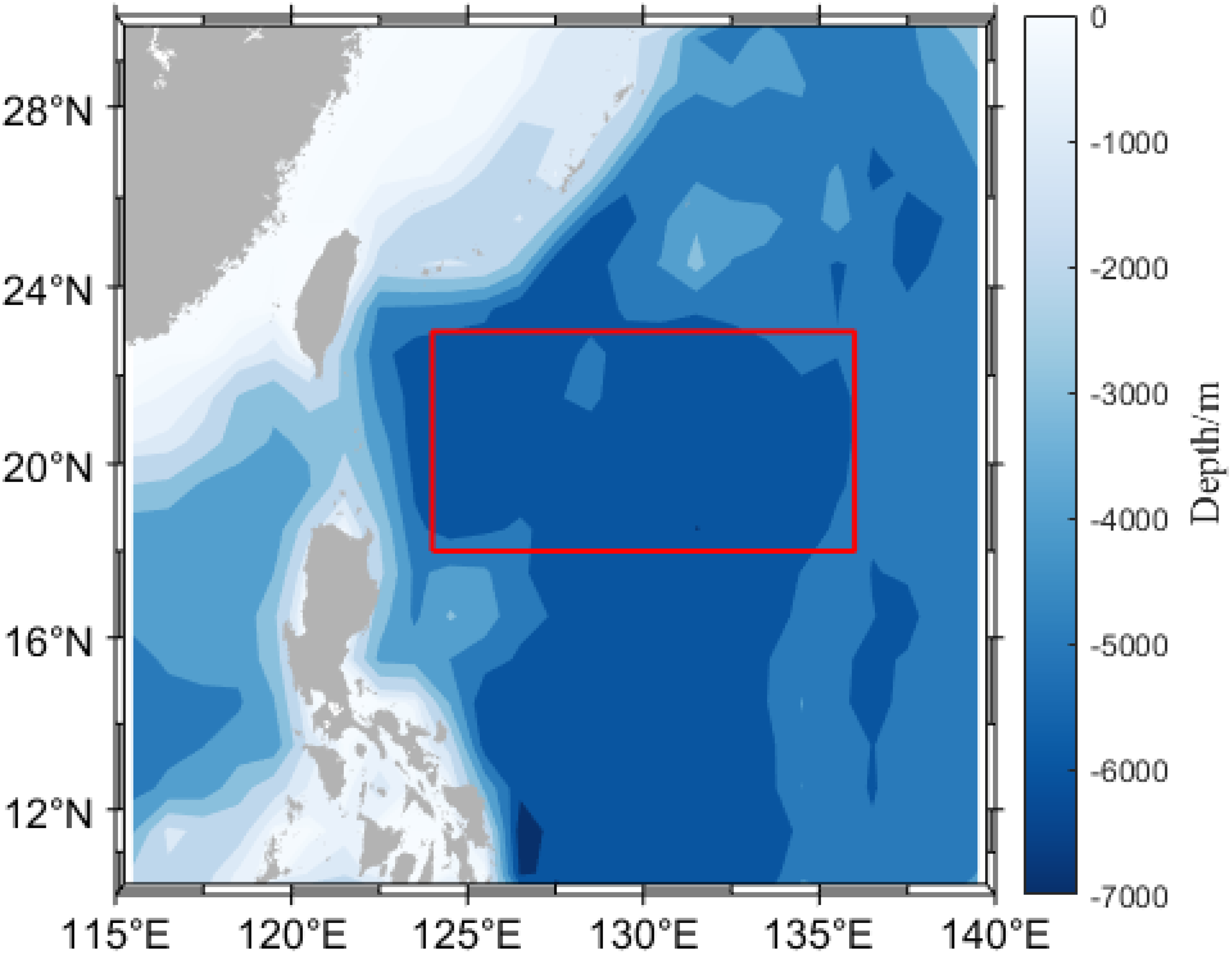
Schematic of the area east of the Luzon Strait, with the experimental area marked in red.
The dataset of sea surface environmental parameters utilized satellite altimeter data, with sea surface temperature (SST) sourced from NOAA and sea level anomalies (SLA) and eddy kinetic energy (EKE) sourced from AVISO. To match the resolution of the remote sensing data, this paper selects temperature and salinity reanalysis data with the same resolution from the CMEMS (Copernicus Marine Environment Monitoring Service) platform for use in sound field reconstruction. The data format is presented in Table 1, covering the period from January 1993 to December 2022, spanning 360 months. The spatial coverage ranges from 18° to 23°N and from 124° to 136°E, with a spatial resolution of 0.25° × 0.25°. The temperature-salinity profile is vertically divided into 75 layers.
Table 1
| Data Name | Data Source | Area | Time Period | Resolution |
|---|---|---|---|---|
| SST | NOAA | 18°-23°N 124°-136°E |
January 1993 - December 2022 | |
| SLA | AVISO | |||
| EKE | ||||
| Temperature and salinity | CMEMS |
Data types.
Sound speed and average density were calculated using functions from the Seawater Toolkit. The sound speed was computed using the UNESCO algorithm (Chen and Millero, 1977), and the specific empirical formula is provided in reference Wong and Zhu, 1995.
2.2 Sound speed reconstruction method
2.2.1 3dCNN-DEN model
The ocean interior exhibits various complex and multiscale dynamic phenomena, which alter the distribution of the sound speed field, disturb the SSP, and affect the paths of sound wave propagation. These phenomena exert a significant and complex influence on the acoustic field structure. Solely using sea surface environmental parameters may limit the reconstruction accuracy of full ocean-depth sound speeds. Therefore, this study abandons the traditional sEOF method and incorporates both sea surface environmental information (SST, SLA, and EKE) and underwater average density to improve accuracy. According to the theoretical formula for sound speed, the phase velocity of sound waves in a compressible medium is expressed as:
where is seawater density, and are the isobaric and isochoric specific heats of seawater, and is the isothermal compressibility of seawater. As shown in Equation 1, the sound speed in seawater is closely related to its density, this paper introduces the average density as underwater information for sound speed reconstruction. To eliminate the influence of seasonal signals, the background density field is calculated using a multi-year seasonal average rather than a simple annual mean climatology. Additionally, with the capability of CNNs to process spatial fields, a region-oriented reconstruction model for full ocean-depth 3D sound speed fields, the 3dCNN-DEN model, is established.
2.2.1.1 Introduction of CNN
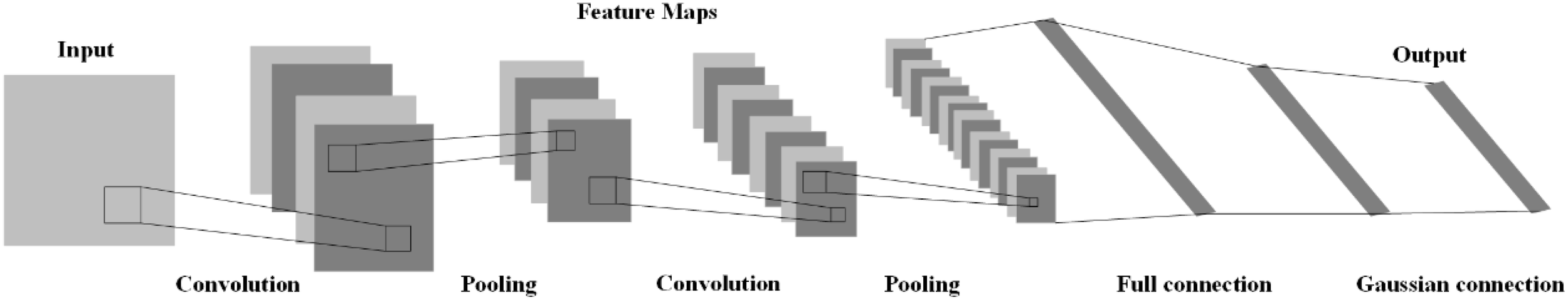
A CNN is a deep feedforward neural network characterized by local connections and weight sharing, with their architecture illustrated in Figure 2. CNNs utilize multiple convolutional layers, pooling layers, and fully connected layers to automatically extract and learn features from data, eliminating the need for manually designed feature extractors. This enhances the efficiency of processing complex data. The convolution operation, through its local receptive capabilities, effectively captures local features in the data. The parameter-sharing mechanism significantly reduces the number of parameters by sliding the convolutional kernel across the entire dataset, lowering both computational and storage demands. Moreover, pooling layers improve the spatial invariance of features, making the model more robust to translation and scaling variations.
Figure 2
CNN structure.
This study selects CNN for sound field reconstruction based on three primary reasons: Firstly, CNNs exhibit significant advantages in processing multidimensional nonlinear data, effectively extracting deep features from sea surface environmental factor fields and average density fields. Secondly, the local perception and multi-scale feature extraction capabilities of CNNs enable them to capture the spatial heterogeneity of marine environments, thereby optimizing the accuracy of sound field reconstruction. Additionally, through convolution operations, CNNs reduce data redundancy and dimensionality, significantly enhancing computational efficiency.
2.2.1.2 Reconstruction technology process
Based on sea surface environmental factors (SST, SLA, and EKE) and incorporating underwater information (average density) as input parameters for sound speed reconstruction, this study developed a region-oriented, full ocean-depth 3D sound speed field reconstruction model (3dCNN-DEN) using the CNN. The technical process is illustrated in Figure 3.
-
Data Preprocessing: Data interpolation and matching are performed to align the temporal and spatial dimensions of the satellite remote sensing data and CMEMS reanalysis data. The underwater sound speed field is calculated with the Seawater Toolkit and the average density is calculated based on historical data as background field.
-
Model Input and Output Determination: The modeling focuses on spatial fields, with sea surface environmental information fields (SST, SLA, and EKE) and average density fields at various depths serving as inputs, while the sound speed fields at various depths are used as outputs. The dataset is divided into training and test sets.
-
Network Training: The CNN establishes a mapping between inputs and outputs. Parameters are continuously adjusted using the training set to optimize the model.
-
Sound Speed Reconstruction: The sea surface information from the test set is fed into the trained model, and the sound speed field is reconstructed layer by layer.
Figure 3
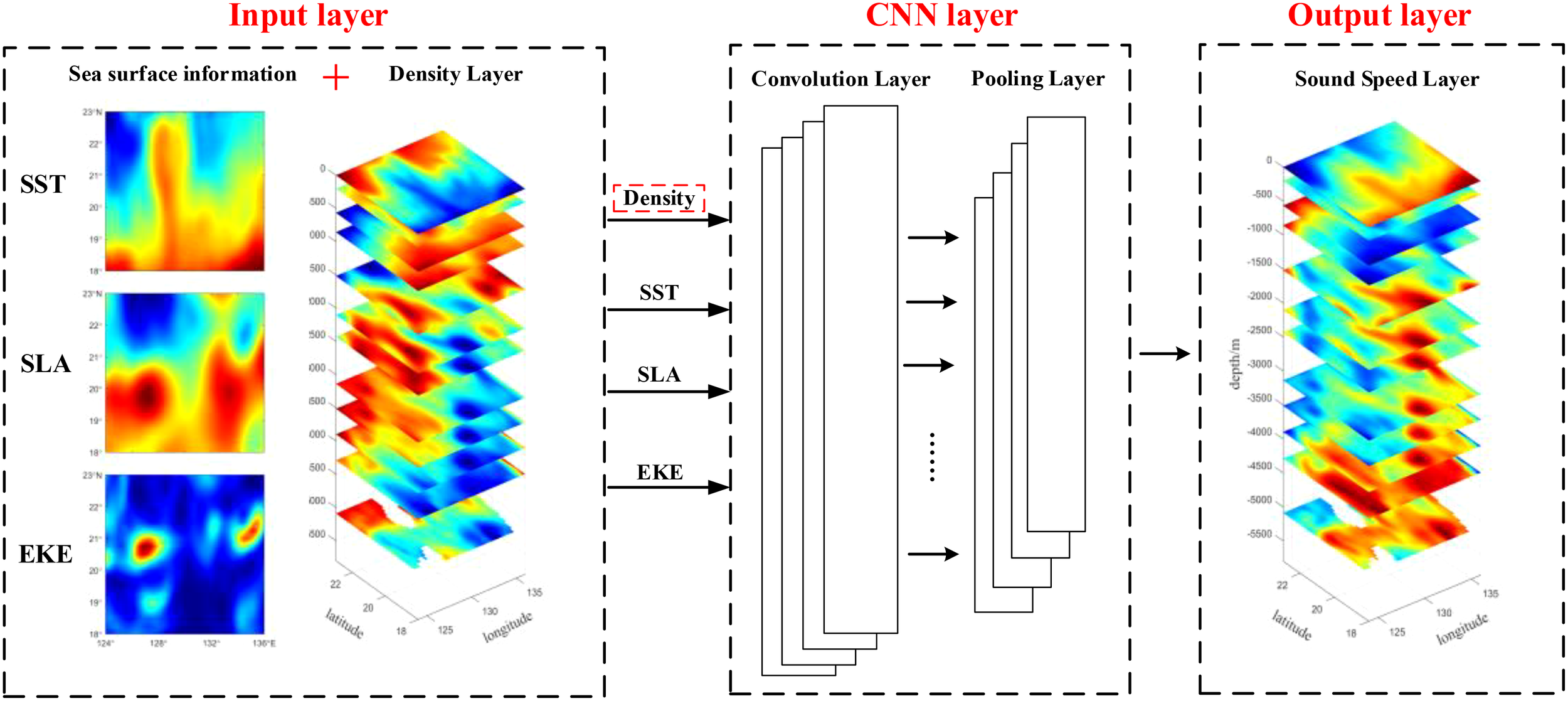
Technical process diagram of 3dCNN-DEN.
2.2.2 Models for comparative analysis
To validate the improvements of the model proposed in this paper, three different sound speed reconstruction models were analyzed and compared: the traditional sEOF-r method, the sEOF-CNN method, and the 3dCNN method. The root mean square error (RMSE) and the mean absolute error (MAE) were used as metrics to measure the error between the estimated sound speed values and the test samples.
2.2.2.1 sEOF-r method
The primary goal of the EOF method is to separate the temporal and spatial variable functions in the SSP, describing the spatiotemporal variations of the SSP using as few modal basis functions as possible. Integrate all SSPs into a sound speed profile matrix , where M represents the number of vertical layers in the SSP (M=75), and N represents the temporal layers of SSPs within the region. By performing EOF decomposition on the SSP matrix , this matrix can be approximately expressed as:
where K is the number of EOFs selected for computation, is the empirical orthogonal coefficient, is the EOF base function, and represents the mean SSP. The selection of the order depends on the variance contribution rate of each mode, with the cumulative variance contribution rate of the first K eigenvectors is given by Equation 3:
Research has shown that when the cumulative variance contribution rate of the first three EOFs (Q) is 88%, reliable reconstruction results can be obtained (Lu et al., 2020).
In the traditional sEOF-r method, the EOF coefficients are typically computed for each location’s SSP matrix based on Equation 2. Following the work of Chen et al. (2018) and Liu et al. (2023, 2024), the relationships between SST, SLA, and EKE with SSP are significant. Therefore, this study constructs a univariate linear regression between the sea surface parameters (SST, SLA, and EKE) and the temporal coefficients of the EOFs. The least squares estimation of the fitting coefficients is obtained, and the linear regression relationship is expressed by Equation 4:
2.2.2.2 sEOF-CNN method
It is well known that the ocean system is complex and nonlinear, and using a linear framework to reconstruct the SSP inevitably introduces systematic errors. To address this limitation, this study incorporates deep learning techniques to capture nonlinear relationships between variables, proposing the sEOF-CNN method (see Figure 4 for the detailed reconstruction process). In the developed sEOF-CNN framework, we establish a supervised learning architecture where sea surface parameters (SST, SLA, and EKE) serve as input features. The CNN is employed to model the nonlinear relationship between these parameters and the principal components (PC1, PC2, PC3) derived from EOF decomposition. In this model, the EOF temporal coefficients serve as the target output variables, while the sea surface environmental parameters constitute the input feature space. Thus, the primary objective of this model is to train a CNN capable of accurately predicting EOF temporal coefficients based on sea surface environmental parameters. Notably, the predicted EOF temporal coefficients generated by the trained CNN model are directly utilized for SSP matrix reconstruction without further involvement in the training process. The final reconstruction involves: (1) linear combination of the predicted temporal coefficients with EOF spatial modes, and (2) superposition with the climatological mean sound speed field, thereby achieving complete three-dimensional sound speed field reconstruction.
Figure 4
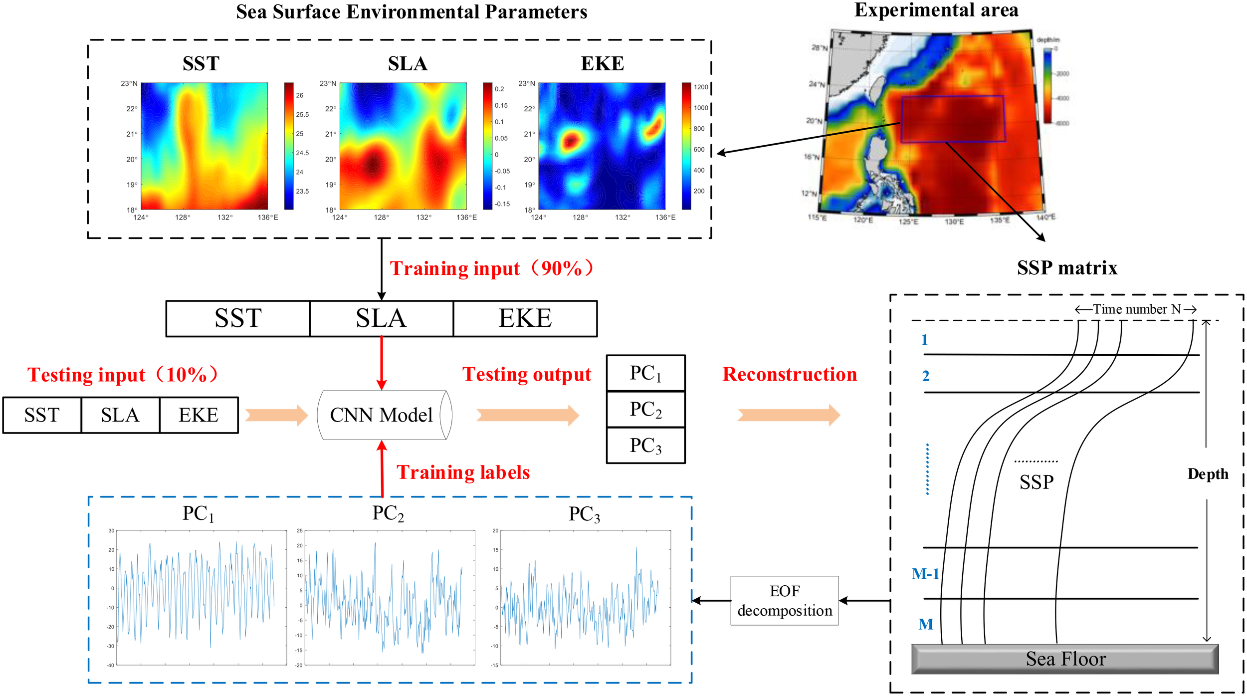
Technical process of the sEOF-CNN method.
2.2.2.3 3dCNN method
To further evaluate the improvement in sound speed reconstruction by incorporating underwater average density, this paper builds the 3dCNN model. Unlike the 3dCNN-DEN model, which incorporates the underwater density field, the 3dCNN model directly uses the sea surface environmental factors (SST, SLA, and EKE) as input for regional 3D sound speed field reconstruction. The 3dCNN model follows a similar technical process as the 3dCNN-DEN model, with the only difference being the inclusion of density as a model input.
3 Modeling and experimental analysis
3.1 Data preprocessing
This study selects the region east of the Luzon Strait (18°-23°N, 124°-136°E) as the research area. The SLA and EKE data from AVISO, SST data from NOAA, and temperature-salinity data from CMEMS share the same resolution. However, there is a 0.125° difference in the grid latitude and longitude between these datasets, resulting in spatial mismatches between the sea surface remote sensing data and the temperature-salinity profile data. To address this issue, the surrounding sea surface data points around each CMEMS grid point are averaged, and masking treatments are applied to handle invalid values at various depths. This process ensures spatial consistency among the four data types, all with a resolution of 0.25° × 0.25°.
Ninety percent of the dataset, covering the period from January 1993 to December 2019 (a total of 27 years with a temporal resolution of one month), are allocated as the training set. The remaining ten percent, spanning from January 2020 to December 2022 (a total of 3 years with a monthly temporal resolution), are designated as the testing set. The reconstruction capability and validation of the 3dCNN-DEN model are assessed based on the specified procedures.
3.2 Sound speed reconstruction modeling process
The key step in the 3D sound speed field reconstruction methods based on CNN (the 3dCNN method and 3dCNN-DEN method) is the construction of the CNN. This study uses Matlab’s Deep Learning Toolbox to build a five-layer network. The first layer is the input layer, where the data are normalized and flattened before being processed. The second layer is a convolutional layer, with a kernel size of 3×1, generating 16 convolutions. The third layer is a pooling layer, with a kernel size of 2×1 and a stride of 2. The fourth layer is a fully connected layer consisting of 50 neurons. Finally, the fifth layer is the regression layer, used to calculate loss values.
For the station-by-station SSP reconstruction methods based on the EOF method (sEOF-r method and sEOF-CNN method), the critical aspect is selecting the appropriate EOF modal order for sound speed. As shown in Table 2, the variance contribution rate of the first three modes following sound speed EOF decomposition is 94.29%, indicating that only the temporal coefficients of these three modes are needed to meet the SSP reconstruction requirements.
Table 2
| Mode number | 1 | 2 | 3 | 4 | 5 |
|---|---|---|---|---|---|
| Variance contribution rate | 64.50% | 21.00% | 8.79% | 3.04% | 0.99% |
Variance contribution rates of the first five modes.
3.3 Analysis of sound speed reconstruction results
A comparative analysis of the reconstruction performance of four methods was conducted, and Figure 5 presents the MAE and RMSE of the reconstructed sound speed at various depth layers. Overall, the CNN-based sound speed field reconstruction models (3dCNN-DEN and 3dCNN) outperform the traditional grid-by-grid SSP reconstruction models (sEOF-CNN and sEOF-r). The EOF method’s use of principal mode extraction for sound speed modeling results in some information loss, thereby reducing reconstruction accuracy.
Figure 5
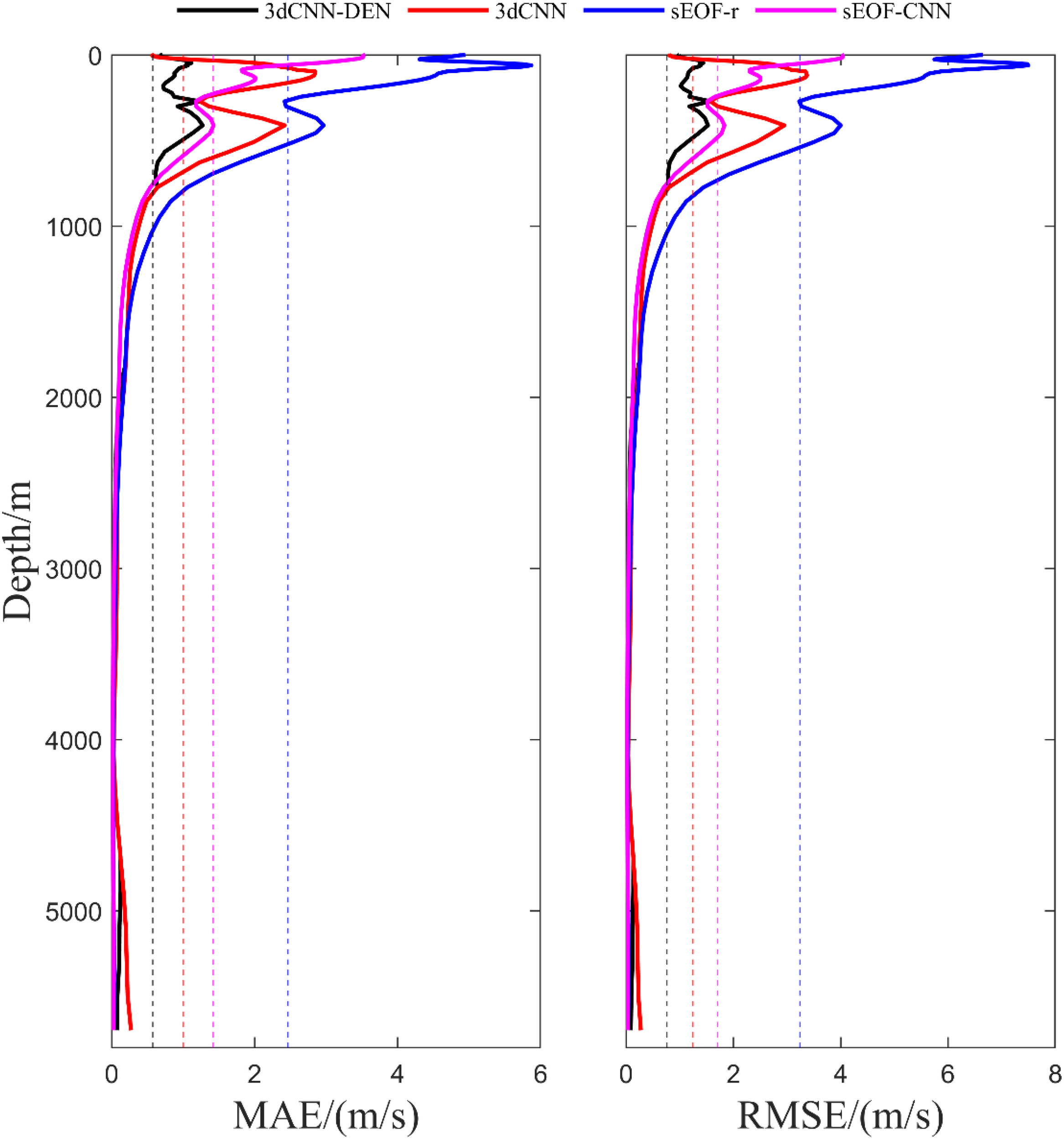
Average MAE and RMSE of sound speed at various depth layers for four sound speed reconstruction methods, with the dashed lines in corresponding colors representing the mean sound speed error for each method.
The improvements in reconstruction capability presented by the models proposed in this paper are particularly notable at depths shallower than 1200 m, with significant gains at depths shallower than 100 m. SSP reconstruction in shallow waters faces multiple challenges: boundary effects, tidal mixing, wave stirring, and intense air-sea interactions collectively induce high dynamism and spatial heterogeneity in vertical sound speed distributions. Conventional EOF methods suffer from inherent limitations, exhibiting reduced modal convergence in nonstationary fields (typically with the first three modes explaining<65% variance). Compounded by the scarcity of historical profile data in shallow waters (only 20-30% of deep-water quantities), neural network training encounters small-sample constraints, jointly contributing to increased SSP reconstruction errors. The proposed 3dCNN-DEN model innovatively incorporates mean seawater density as a key input parameter, enabling multimodal data fusion with sea surface environmental factors. This approach significantly enhances modeling accuracy for temperature-salinity-pressure coupling effects on sound speed. Experimental results demonstrate that in shallow waters (<100 m), 3dCNN-DEN achieves a sound speed error of 0.8398 m/s, representing reductions of 18.5%, 74.7%, and 82.6% compared to the baseline models 3dCNN (1.031 m/s), sEOF-CNN (3.3229 m/s), and sEOF-r (4.8392 m/s), respectively, confirming its superior performance in shallow regions. In intermediate depths (100–650 m), the sEOF-CNN method exhibits a relative advantage, with a reconstruction error of 1.5771 m/s771tru lower than 3dCNN’s 2.1264 m/s. Notably, by incorporating vertical seawater density information, 3dCNN-DEN further reduces the error to 0.9234 m/s, achieving a 56.6% improvement over 3dCNN. As depth increases, performance differences between models gradually diminish: in deep waters (>780 m), all models stabilize with errors below 1 m/s, and at 1150 m, errors converge to within 0.5 m/s, indicating stronger spatiotemporal stability in deep-water sound speed fields.
Table 3 shows the average reconstruction accuracies of the four models, ranked as 3dCNN-DEN > 3dCNN > sEOF-CNN > sEOF-r. The 3dCNN-DEN model proposed in this paper improves reconstruction accuracy by 77.1% compared to the traditional sEOF-r method. Among the two SSP reconstruction models based on the EOF method, the nonlinear framework constructed using deep learning (sEOF-CNN) outperforms the traditional linear framework (sEOF-r), with a 42.4% improvement in model reconstruction accuracy. Comparing the two sound speed field reconstruction models based on CNN, the introduction of underwater average density enhances the reconstruction accuracy by 42.4%, significantly boosting the model’s performance.
Table 3
| Reconstruction model | MAE (m/s) | RMSE (m/s) |
|---|---|---|
| sEOF-r | 2.5169 | 4.1527 |
| sEOF-CNN | 1.4498 | 2.2914 |
| 3dCNN | 0.9998 | 1.2427 |
| 3dCNN-DEN | 0.5759 | 0.7572 |
The vertical average MAE and RMSE of four sound speed reconstruction models.
Table 4 presents the research efforts of several scholars in the field of sound speed reconstruction. It is evident that the current mainstream approach involves combining sEOF with machine learning, and regardless of the specific machine learning framework used, the typical accuracy of SSP reconstruction models based on sEOF remains around 1~2 m/s. Although sound speed reconstruction errors can be reduced to below 1 m/s in certain regions, the overall development trend has reached a bottleneck. The 3dCNN-DEN model proposed in this study departs from traditional point-by-point reconstruction methods by innovatively incorporating average density fields as model inputs. This reduces the overall sound speed reconstruction error to 0.7572 m/s, significantly enhancing the precision and efficiency of underwater sound speed reconstruction. Furthermore, CNNs have demonstrated exceptional performance in sound field reconstruction tasks, providing new tools and methodologies for marine acoustic research.
Table 4
| Author | Method | RMSE (m/s) | Region |
|---|---|---|---|
| Li et al. (2022) | sEOF-SOM | 1.69 | Southeast Indian Ocean |
| Feng et al. (2024) | sEOF-MLR | 1.63 | The South China Sea |
| sEOF-SVR | 1.53 | ||
| sEOF-XGBoost | 1.16 | ||
| Zhao et al. (2024) | sEOF-LSTM | 1.76 | |
| Liu et al. (2024) | sEOF-GRNN | 1.50 | Luzon Strait |
The related work of other scholars.
To further compare the reconstruction effects of the four sound speed reconstruction methods, Figure 6 presents the sound speed reconstruction errors at different depths. The sEOF-r method exhibits large overall sound speed errors, with a scattered error distribution, and some regions showing sound speed errors greater than 10 m/s. In contrast, the errors of the sEOF-CNN, 3dCNN, and 3dCNN-DEN methods were relatively smooth in space and better represent the spatial distribution characteristics of sound speed. At near-surface layers, the CNN-based 3D sound speed field reconstruction models significantly outperform the traditional grid-by-grid SSP reconstruction models, particularly in the upper layers of the sea. At depths of 97 m, 120 m, and 411 m, the reconstruction accuracy of the sEOF-CNN method is slightly better than that of the 3dCNN method. Under the same sea surface environmental input data, the 3dCNN model’s reconstruction capability in the upper ocean layers could be improved, as is evident from the MAE and RMSE distribution in Figure 5. By incorporating average density field, the 3dCNN-DEN method further enhances the model’s reconstruction accuracy, especially in the upper ocean layers, where a substantial reduction in sound speed error is observed.
Figure 6
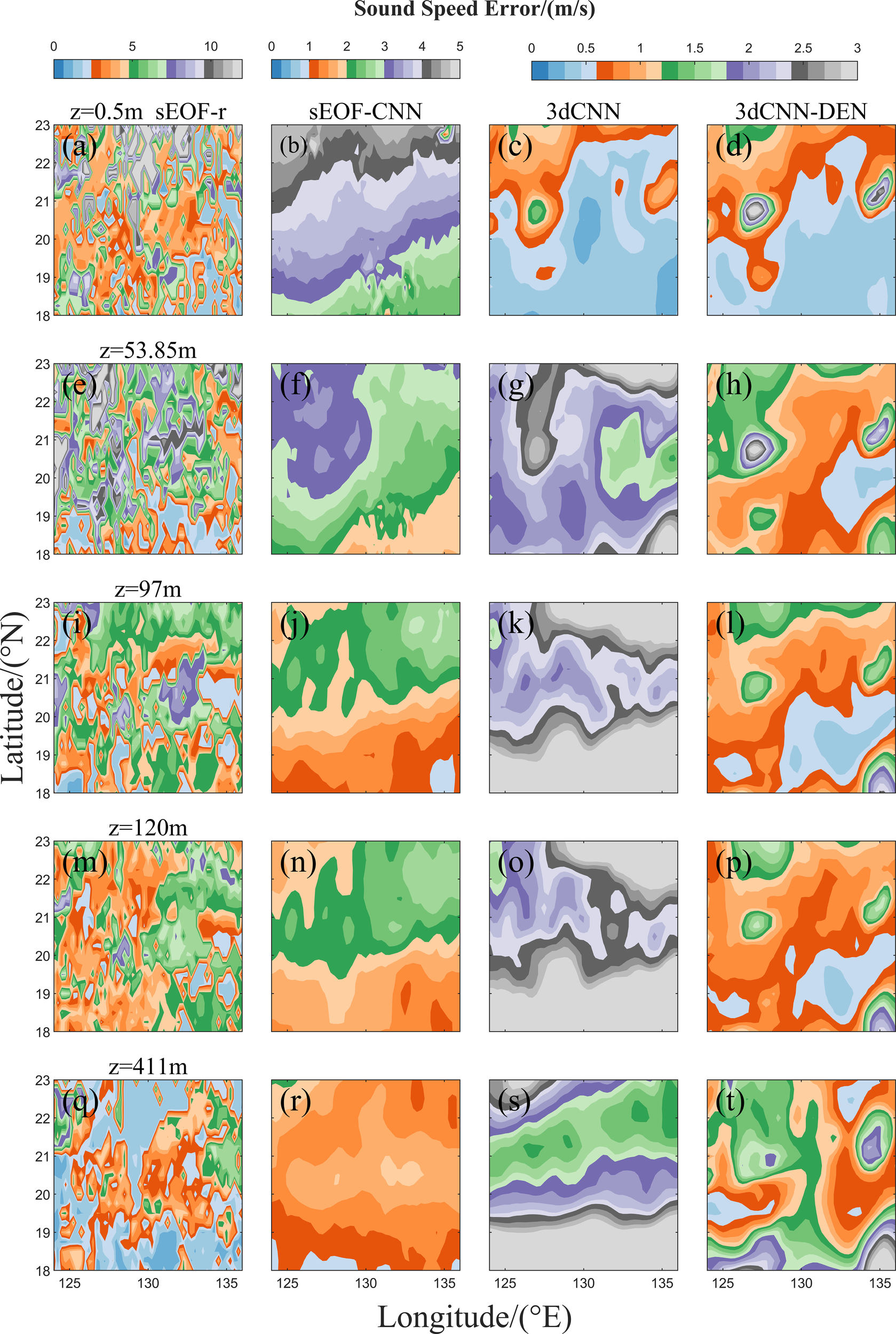
(a–t) Sound speed errors at different depths for the four sound speed reconstruction methods. Columns 1–4 represent errors for sEOF-r, sEOF-CNN, 3dCNN, and 3dCNN-DEN, respectively, and rows 1–5 show errors at depths of 0.5 m, 53.85 m, 97 m, 120 m, and 411 m.
Figure 7 shows the full ocean-depth average MAE and RMSE distribution for the four sound speed reconstruction methods, which mirrors the pattern observed in Figure 6. The reconstruction accuracies of the models are ranked: 3dCNN-DEN > 3dCNN > sEOF-CNN > sEOF-r. The sEOF-r method exhibits larger overall sound speed errors with a scattered distribution, while the other models display smoother errors in space, better restoring the overall spatial distribution characteristics of sound speed, but there are still some differences in the fine structure of the sound speed distribution across regions. At the same time, because the reconstruction is performed on a per-grid-point basis, it is challenging to accurately depict the regional impacts of large-scale and mesoscale oceanic dynamical phenomena on sound field reconstruction. Compared to the 3dCNN model, the inclusion of vertical seawater density significantly enhances the reconstruction capability of the 3dCNN-DEN model. Notably, the areas with larger reconstruction errors are concentrated in two circular regions between 20°-21.5°N, 125.5°-127°E, and 20.5°-22°N, 133°-136°E. We initially guessed that the abnormal error was caused by the perennial existence of mesoscale eddies in these two regions.
Figure 7
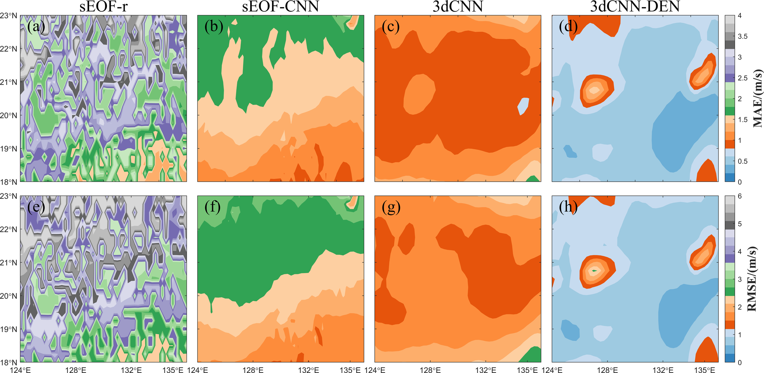
(a–h) Full ocean-depth average MAE and RMSE distribution for the four sound speed reconstruction methods.
3.4 Anomalous error analysis and discussion
Although the 3dCNN-DEN model developed in this study has significantly improved overall sound speed reconstruction accuracy, certain areas exhibit notably large errors. To verify the previously mentioned hypothesis about anomalous error regions, Figure 8a shows the multi-year average EKE distribution of the study area. It is evident that in two circular regions—20°–21.5°N, 125.5°–127°E and 20.5°–22°N, 133°–136°E—the EKE values are significantly higher than in other areas, indicating the persistent presence of two strong mesoscale eddies. Meanwhile, we performed a multi-year average of the SLA and surface current field in this region from the testing set and identified them using the traditional Okudo-Weiss (OW) algorithm (Isern et al., 2003). It was found that these two circular regions highly coincide with the areas where mesoscale eddies are located (the black curves in Figure 8a represent the boundaries of the mesoscale eddies, and the white stars indicate the eddy centers). This indicates that within the influence region of mesoscale eddies, the sound speed reconstruction error of the 3dCNN-DEN model is significantly larger. To more intuitively demonstrate the impact of mesoscale eddies on sound speed reconstruction, within the mesoscale eddy at 20°–21.5°N, 125.5°–127°E, five stations (S1-S5) were selected, while two stations (S6-S7) were chosen outside the eddy. Figures 8b–h display the variations in the reconstructed sound speed with depth at these stations, and Table 5 presents the average MAE of the reconstructed sound speed. For the grid-by-grid SSP reconstruction method based on the EOF approach, the sound speed reconstruction accuracy shows no significant difference inside versus outside the mesoscale eddy. However, for the 3D CNN-based reconstruction methods, the errors at stations within the eddy are significantly larger, particularly for the 3dCNN-DEN model proposed here. Despite its high overall accuracy, the performance difference between inside and outside the eddy is most pronounced for the 3dCNN-DEN model.
Figure 8
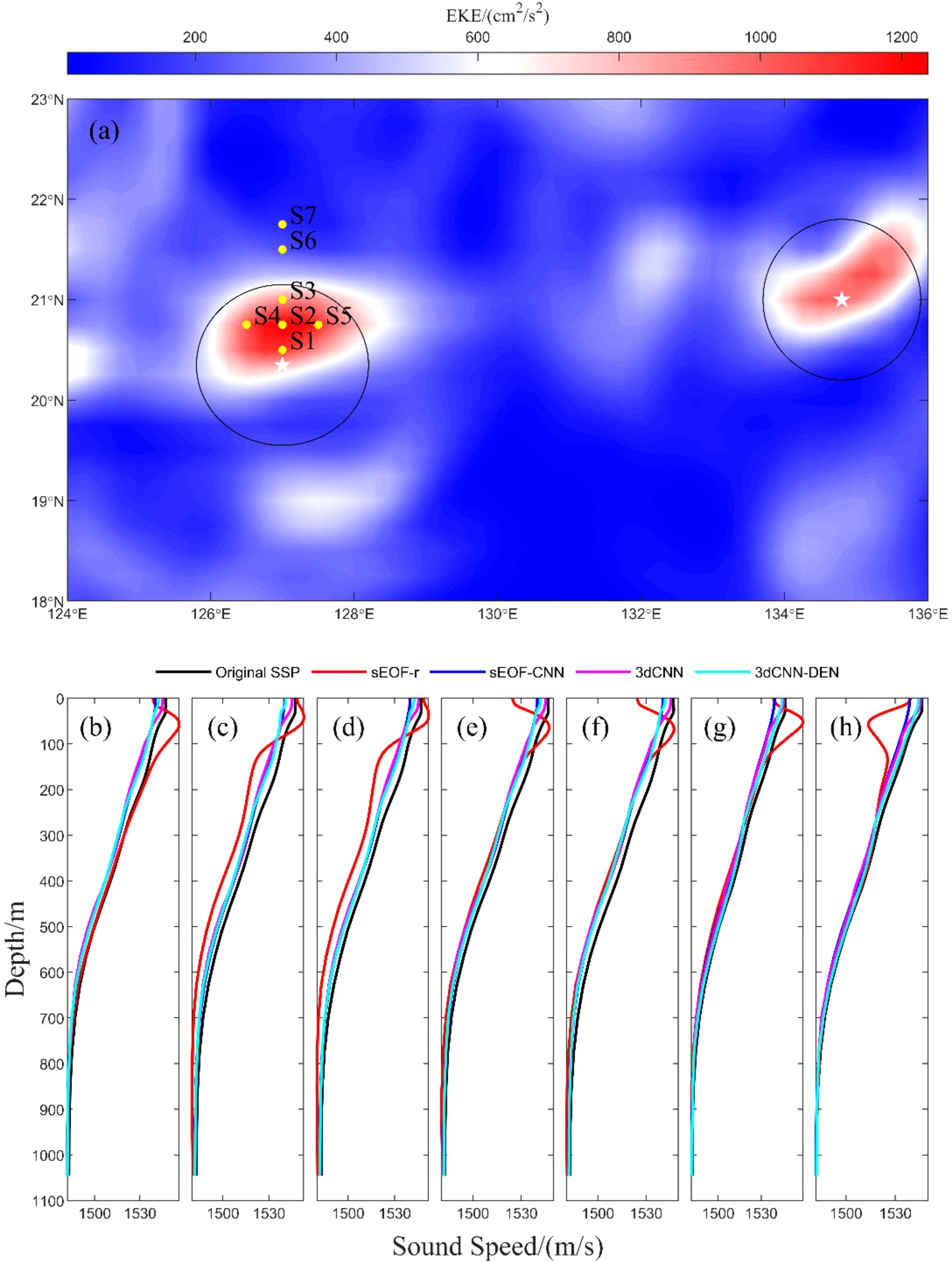
(a) Distribution of EKE and mesoscale eddies within the study area; (b–h) Comparison of reconstructed SSP using four methods at the seven selected stations.
Table 5
| Station | MAE/(m/s) | ||||
|---|---|---|---|---|---|
| sEOF-r | sEOF-CNN | 3dCNN | 3dCNN-DEN | ||
| Inside eddy | S1 | 4.8183 | 4.9290 | 3.6080 | 4.3852 |
| S2 | 9.0384 | 4.9502 | 3.4620 | 4.3205 | |
| S3 | 6.9195 | 5.4592 | 3.6954 | 4.3032 | |
| S4 | 9.0384 | 4.9502 | 3.4630 | 4.3205 | |
| S5 | 9.5852 | 5.3678 | 3.9052 | 4.9532 | |
| Average MAE inside eddy | 7.8800 | 5.1313 | 3.6265 | 4.4565 | |
| Outside eddy | S6 | 5.4698 | 5.3619 | 3.0218 | 2.3544 |
| S7 | 9.8914 | 5.0730 | 2.5648 | 1.8562 | |
| Average MAE outside eddy | 7.6806 | 5.2175 | 2.7933 | 2.1068 | |
Average MAE of reconstructed sound speed for the four sound speed reconstruction methods at seven stations.
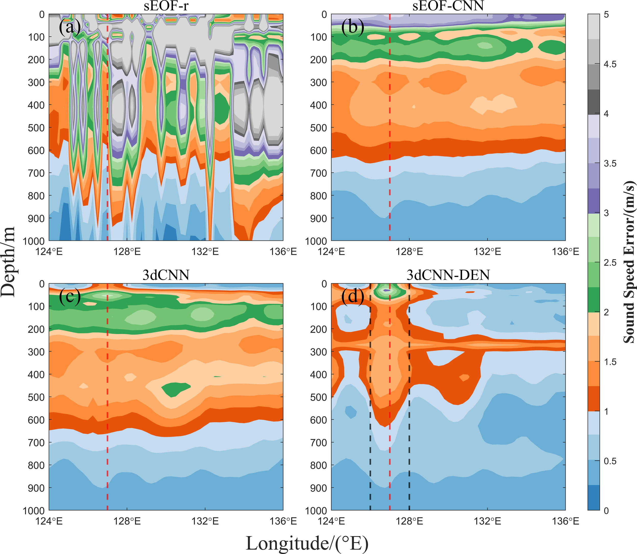
To further analyze the impact of mesoscale eddies on the reconstruction performance of the 3dCNN-DEN model, cross-sectional analyses were conducted along both the longitudinal and latitudinal axes at the center of the mesoscale eddy located at 20.75°N, 127°E, as shown in Figures 9, 10. In the 127°E cross-section (Figure 9), the mesoscale eddy extends between 20° and 21.5°N, as indicated by the black dashed line in Figure 9d, with the red dashed line marking the eddy center. It was observed that the large error areas in the reconstructed sound speed using the sEOF-r and sEOF-CNN methods are concentrated in the upper ocean layer (0–100 m) and show little correlation with the eddy region. The average MAE for sound speed within this depth range is 5.4792 m/s and 3.2997 m/s, respectively, which is significantly higher than the average MAE of the 3dCNN and 3dCNN-DEN models at the same depth (1.4758 m/s and 1.2857 m/s, respectively).
Figure 9
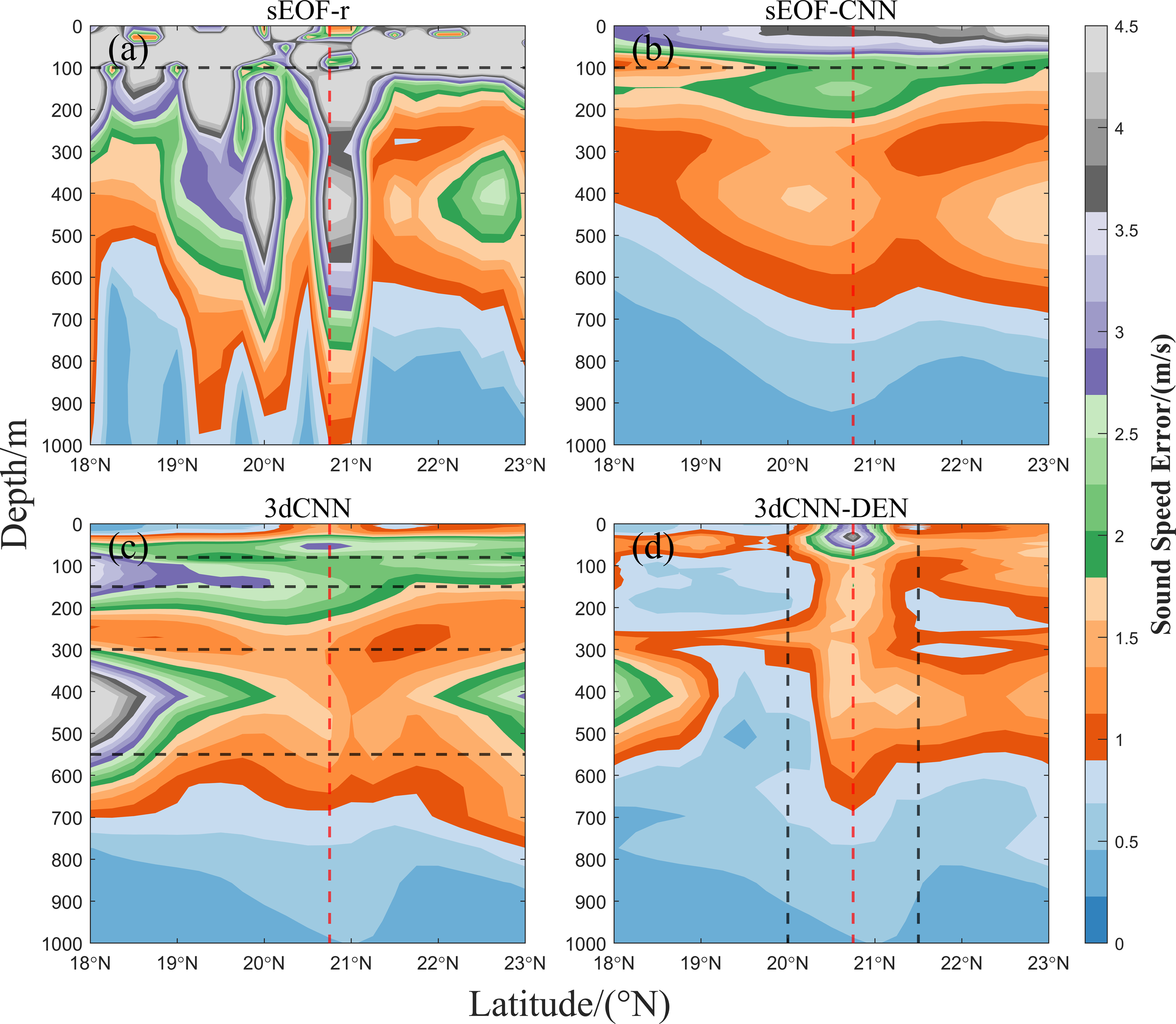
(a–d) Sound speed error distribution for the four sound speed reconstruction methods at the 127°E cross-section.
Figure 10
(a–d) Sound speed error distribution for the four sound speed reconstruction methods at the 20.75°N cross-section.
The large error areas in the reconstructed sound speed from the 3dCNN method are not located within the mesoscale eddy range but are instead concentrated between the 100–160 m and 300–500 m depths, closely aligning with the higher MAE and RMSE values shown in Figure 5. The average MAE for sound speed in these depth ranges is 2.4393 m/s and 1.9288 m/s, respectively. Conversely, the 3dCNN-DEN model’s large error areas are concentrated within the mesoscale eddy’s range, extending from the surface down to 500 m, and possibly affecting depths of up to 1000 m. The highest average MAE at the eddy center is 2.3232 m/s. Within the mesoscale eddy, the average MAE for the reconstructed sound speed is 1.5058 m/s, slightly higher than the 0.9548 m/s outside the eddy region.
For the 20.5°N cross-section (Figure 10), the mesoscale eddy’s range is between 125.5° and 127°E, as indicated by the black dashed line in Figure 10d, with the red dashed line marking the eddy center. The error distribution across the four sound speed reconstruction methods at the corresponding depths is similar to that in Figure 9. The mesoscale eddy has little impact on the reconstruction accuracy of the sEOF-r, sEOF-CNN, and 3dCNN methods, but it significantly affects the accuracy of the 3dCNN-DEN method. The affected depth ranges from the surface down to 500 m, with possible effects reaching as deep as 1000 m. At the eddy center, the average MAE of the reconstructed sound speed reaches a maximum of 1.9244 m/s.
All in all, the reconstruction accuracy of the 3dCNN-DEN model is significantly influenced by mesoscale eddies, with regions of anomalously high sound speed errors closely matching the depth and range of eddies. One possible explanation for this is that density structure within mesoscale eddies differs significantly from the average density. By contrast, in regions outside of mesoscale eddies, the 3dCNN-DEN model exhibits significantly higher reconstruction accuracy than the 3dCNN model, further demonstrating that the inclusion of underwater average density greatly enhances the model’s reconstruction capabilities. This finding provides a crucial direction for the optimization of future ocean models, particularly in handling complex ocean dynamic phenomena, where the incorporation of vertical density parameters may prove essential. Given the significant role of mesoscale eddies in ocean dynamics and their impact on sound speed fields, this is critical for applications such as ocean acoustic detection and ocean circulation modeling. Therefore, in marine environmental research, special attention should be paid to the temperature-salinity characteristics of mesoscale eddies and their influence on model accuracy to enhance the precision of ocean observations and predictions.
4 Conclusion
This paper proposes a region-oriented reconstruction model for 3D sound speed field using the CNN (3dCNN-DEN). The model incorporates not only sea surface environmental information (SST, SLA, and EKE) but also underwater information (average density) for reconstruction. To test the validity of the proposed model, we compared it with traditional sEOF methods (sEOF-r and sEOF-CNN) and a sound speed field reconstruction model based on deep learning (3dCNN). The results showed the following:
-
The 3D sound speed field reconstruction models based on CNN (3dCNN-DEN and 3dCNN) significantly outperformed the grid-by-grid SSP reconstruction models based on EOF (sEOF-r and sEOF-CNN), particularly in the upper seawater layers (0–100 m), where reconstruction errors were smaller. The 3dCNN-DEN model achieved an average MAE of 0.5759 m/s and an average RMSE of 0.7572 m/s, representing reductions of 77.1% in both MAE and RMSE values compared to the sEOF-r method. Besides, the reconstruction errors of 3dCNN-DEN are smoother and more consecutive in space, which can better represent the spatial distribution characteristics of sound speed.
-
Compared to the 3dCNN model, the 3dCNN-DEN model further improved reconstruction accuracy by 42.4%, demonstrating that the inclusion of underwater average density significantly enhanced the reconstruction performance. Within strong mesoscale eddies, the density structure usually differs significantly from the average density (that is background field), leading to poorer reconstruction performance within the eddies’ influence range and depth. In the future research, we will focus on proposing a specialized model for the mesoscale eddy and improving SSP reconstruction in mesoscale eddy regions.
Statements
Data availability statement
The original contributions presented in the study are included in the article/supplementary material. Further inquiries can be directed to the corresponding author.
Author contributions
HL: Writing – original draft, Writing – review & editing. YL: Data curation, Investigation, Writing – review & editing. ML: Formal analysis, Methodology, Supervision, Writing – original draft, Writing – review & editing. PW: Data curation, Formal analysis, Methodology, Writing – review & editing. YZ: Data curation, Investigation, Software, Writing – review & editing. KM: Formal analysis, Resources, Validation, Writing – review & editing. XC: Formal analysis, Supervision, Validation, Writing – review & editing.
Funding
The author(s) declare that no financial support was received for the research and/or publication of this article.
Acknowledgments
The SST data were made available on the NOAA web (http://www.emc.ncep.noaa.gov/research/cmb/sst_analysis/). The SLA and EKE data were made available on the AVISO web (ftp://ftp.aviso.altimetry.fr/). The temperature-salinity data were made available on the CMEMS web (https://marine.copernicus.eu/).
Conflict of interest
The authors declare that the research was conducted in the absence of any commercial or financial relationships that could be construed as a potential conflict of interest.
Generative AI statement
The author(s) declare that no Generative AI was used in the creation of this manuscript.
Publisher’s note
All claims expressed in this article are solely those of the authors and do not necessarily represent those of their affiliated organizations, or those of the publisher, the editors and the reviewers. Any product that may be evaluated in this article, or claim that may be made by its manufacturer, is not guaranteed or endorsed by the publisher.
References
1
Alexander P. Duncan A. Bose N. Williams G. (2016). Modelling acoustic propagation beneath Antarctic sea ice using measured environmental parameters. Deep-Sea Res. Part II131, 84–95. doi: 10.1016/j.dsr2.2016.04.026
2
Chen C. Ma Y. L. Liu Y. (2018). Reconstructing sound speed profiles worldwide with sea surface data. Appl. Ocean Res.77, 26–33. doi: 10.1016/j.apor.2018.05.002
3
Chen C. T. Millero F. J. (1977). Speed of sound in seawater at high pressures. J. Acoustical Soc. America62, 1129–1135. doi: 10.1121/1.381646
4
Chen C. Yang K. D. Duan R. Ma Y. L . (2017). Acoustic propagation analysis with a sound speed feature model in the front area of Kuroshio Extension. Appl. Ocean Res.68, 1–10. doi: 10.1016/j.apor.2017.08.001
5
Chen W. Zhang Y. C. Liu Y. Y. Ma L. N. Wang H. D. Ren K. J. et al . (2022). Parametric model for eddies-induced sound speed anomaly in five active Mesoscale Eddy regions. J. Geophysical Research: Oceans127, 1–23. doi: 10.1029/2022JC018408
6
Feng X. Tian T. Zhou M. Z. Sun H. X. Li D. Z. Tian K. et al . (2024). Sound speed inversion based on multi-source ocean remote sensing observations and machine learning. Remote Sens.16, 814. doi: 10.3390/rs16050814
7
Fox D. N. Teague W. J. Barron C. N. Carnes M. R. Lee C. M. (2002). The modular ocean data assimilation system (MODAS). J. Atmospheric Oceanic Technol.19, 240–252. doi: 10.1175/1520-0426(2002)019<0240:TMODAS>2.0.CO;2
8
Isern F. J. Garcia L. E. Font J. (2003). Identification of marine eddies from altimetric maps. J. Atmospheric Oceanic Technol.20, 772. doi: 10.1175/1520-0426(2003)20<772:IOMEFA>2.0.CO;2
9
Jain S. Ali M. M. (2006). Estimation of sound speed profiles using artificial neural networks. IEEE Geosci. Remote Sens. Lett.3, 467–470. doi: 10.1109/LGRS.2006.876221
10
Leblanc L. R. Middleton F. H. (1980). An underwater acoustic sound velocity data model. J. Acoustical Soc. America67, 2055–2062. doi: 10.1121/1.384448
11
Li Q. Q. Li H. L. Cao S. L. Yan X. Ma Z. C. (2022). Inversion of the full-depth sound speed profile based on remote sensing data and surface sound speed. Haiyang Xuebao44, 84–94. doi: 10.12284/hyxb2022149
12
Li H. P. Qu K. Zhou J. B. (2021). Reconstructing sound speed profile from remote sensing data: nonlinear inversion based on self-organizing map. IEEE Acess9, 109754–109762. doi: 10.1109/ACCESS.2021.3102608
13
Li B. Y. Zhai J. S. (2022). A novel sound speed profile prediction method based on the convolutional long-short term memory network. J. Mar. Sci. Eng.10, 572. doi: 10.3390/jmse10050572
14
Lin Y. T. Lynch J. F. (2017). Three-dimensional sound propagation and scattering in an ocean with surface and internal waves over range-dependent seafloor. J. Acoustical Soc. America141, 3753. doi: 10.1121/1.4988280
15
Liu Y. Y. Chen Y. Chen W. Meng Z. (2023). Inversion of sound speed profile in the Luzon strait by combining single empirical orthogonal function and generalized regression neural network. IEEE Geosci. Remote Sens. Lett.21, 1502405. doi: 10.1109/LGRS.2024.3379200
16
Liu Y. Y. Chen Y. Meng Z. et al . (2023). Performance of single empirical orthogonal function regression method in global sound speed profile inversion and sound field prediction. Appl. Ocean Res.136, 103598. doi: 10.1016/j.apor.2023.103598
17
Liu L. Peng S. Q. Huang R. X. (2017). Reconstruction of ocean’s interior from observed sea surface information. J. Geophysical Research: Oceans122, 1042–1056. doi: 10.1002/2016JC011927
18
Liu Y. F. Wang Z. J. Zhao S. (2020). Layered-EOFs based adaptive reconstruction of sound velocity profile in multi-beam sounding. Tech. Acoustics39, 372–378. doi: 10.16300/j.cnki.1000-3630.2020.03.020
19
Lu S. L. Liu Z. H. Li H. Li Z. Q. Wu X. F. Sun C. H. et al . (2020). User Manual of Global Ocean Argo Grid Dataset (BOA_Argo), China Argo Real-time Data Center. 28pp.
20
Park J. C. Kennedy R. M. (1996). Remote sensing of ocean sound speed profiles by a perceptron neural network. IEEE J. Oceanic Eng.21, 216–224. doi: 10.1109/48.486796
21
Shen H. Jia Y. L. Zhang X. Liu Q. Y. Chen L. J. (2013). Effect on eddies in the east of the Luzon strait to the Kuroshio and the South China Sea. Periodical Ocean Univ. China43, 9–16. doi: 10.16441/j.cnki.hdxb.2013.06.002
22
Wang J. B. Flierl G. R. Lacasce J. H. (2013). Reconstructing the ocean’s interior from surface data. J. Phys. Oceanography43, 1611–1626. doi: 10.1175/JPO-D-12-0204.1
23
Wong G. S. K. Zhu S. M. (1995). Speed of sound in seawater as a function of salinity, temperature and pressure. J. Acoustical Soc. America97, 1732–1736. doi: 10.1121/1.413048
24
Wu S. L. Li Z. L. Qin J. X. Wang M. Y. Li W. (2022). The effects of sound speed profile to the convergence zone in deep water. J. Mar. Sci. Eng.10, 424. doi: 10.3390/jmse10030424
25
Zhao Y. Xu P. Li G. M. Ou Z. Y. Qu K. (2024). Reconstructing the sound speed profile of South China Sea using remote sensing data and long short-term memory neural networks. Front. Mar. Sci.11. doi: 10.3389/fmars.2024.1375766
Summary
Keywords
sound speed reconstruction, convolutional neural network, average density, empirical orthogonal function method, sea surface environmental information
Citation
Li H, Liu Y, Li M, Wang P, Zhu Y, Mao K and Chen X (2025) A deep learning-based reconstruction model for 3D sound speed field combining underwater vertical information. Front. Mar. Sci. 12:1551823. doi: 10.3389/fmars.2025.1551823
Received
26 December 2024
Accepted
19 May 2025
Published
03 June 2025
Volume
12 - 2025
Edited by
Konstantin Markov, University of Aizu, Japan
Reviewed by
Tien Anh Tran, Seoul National University, Republic of Korea
Ziqi Yu, Toyota Research Institute of North America, United States
Updates
Copyright
© 2025 Li, Liu, Li, Wang, Zhu, Mao and Chen.
This is an open-access article distributed under the terms of the Creative Commons Attribution License (CC BY). The use, distribution or reproduction in other forums is permitted, provided the original author(s) and the copyright owner(s) are credited and that the original publication in this journal is cited, in accordance with accepted academic practice. No use, distribution or reproduction is permitted which does not comply with these terms.
*Correspondence: Ming Li, mingli152@163.com
Disclaimer
All claims expressed in this article are solely those of the authors and do not necessarily represent those of their affiliated organizations, or those of the publisher, the editors and the reviewers. Any product that may be evaluated in this article or claim that may be made by its manufacturer is not guaranteed or endorsed by the publisher.