Unraveling natural carbonate variability in Narragansett Bay, RI using multiple high temporal resolution pH time series

The increase in atmospheric carbon dioxide (CO₂) over the last 200 years has largely been mitigated by the ocean’s function as a carbon sink. However, this continuous absorption of CO₂ by seawater triggers ocean acidification (OA), a process in which water becomes more acidic and more depleted in carbonate ions that are essential for calcifiers. OA is well-studied in open ocean environments; however, understanding the unique manifestation of OA in coastal ecosystems presents myriad challenges due to considerable natural variability resulting from concurrent and sometimes opposing coastal processes—e.g. eutrophication, changing hydrological conditions, heterogeneous biological activity, and complex water mass mixing. Developing a mechanistic understanding of carbonate chemistry variability and its drivers across different time scales is a critical first step in identifying the anthropogenic OA signal against background variability and predicting future OA in coastal systems. This study analyzed high temporal resolution pH data collected during 2022 and 2023 from Narragansett Bay, RI—a mid-sized, urban estuary that since 2005 has undergone a 50% reduction in nitrogen loading—with weekly, discrete bottle samples to verify sensor data. Over a year’s worth of data revealed a distinct diurnal cycle of pH, with pH increasing during the day and decreasing during the night, with an average daily range between 0.05 and 0.1 pH units. Further, we observed a strong seasonal cycles with higher mean pH in winter (8.07 ± 0.15) and lower mean pH in summer (7.72 ± 0.07). By separating the drivers of pH variability into effects from temperature, salinity, water mass mixing, biological activity, and air-sea gas flux, we determined that biological production has the most significant influence on pH from daily to annual timescales and in episodic pH changes. To a lesser extent, the seasonal air-sea CO₂ exchange and temperature cycle further modified pH on monthly to seasonal timescales. The dominant influence of biological activity in modulating pH has allowed Narragansett Bay’s nutrient reductions, which have been successful in increasing bottom water DO and pH conditions, to modestly reduce summertime surface pH through reduced primary production. This study offers an in-depth understanding of Narragansett Bay’s natural carbonate variability and highlights the sensitivity of an estuary to water management policy. These findings will benefit future OA prediction and will ultimately assist in making environmental management decisions in coastal estuaries with implications for multiple coastal stakeholders.

1 Introduction

Since the Industrial Revolution, carbon dioxide (CO₂) emissions from fossil fuel burning and land use changes have increased atmospheric CO₂ from preindustrial levels of around 280 ppm to an annual average of 421 ppm in 2023 (Lan et al., 2023). Since 1850 the ocean has removed 26% of anthropogenic emissions from the atmosphere (Friedlingstein et al., 2022). As the ocean continues to take up excess atmospheric CO₂, a cascade of chemical reactions beginning with CO₂ gas dissolving in water, summarized in Equation 1, increases hydrogen ion concentration ([H⁺]) into the water column, thus lowering pH and reducing carbonate ion concentration. This process is known as ocean acidification (OA) and has decreased global surface ocean pH by more than 0.1 units since the preindustrial age, a change corresponding to a 30-40% increase in [H⁺] (Doney et al., 2009; Feely et al., 2023; Jiang et al., 2019).

$\begin{array}{ll}C{O}_{2(gas)}+H_{2}O\stackrel{K_0}{\rightleftharpoons }{H}_{2}C{O}_3\stackrel{K_1}{\rightleftharpoons }{H}^{+}+HC{O}_3{}^{-}\stackrel{K_2}{\rightleftharpoons }2H^{+}+C{O}_3{}^{2-}& (1)\end{array}$

Ongoing OA research continues to improve our understanding of its drivers in the global ocean and its deleterious effects on the ecological community, particularly calcifying organisms (Orr et al., 2005; Kroeker et al., 2010; Jiang et al., 2019; Kwiatkowski and Orr, 2018). For example, the increased acidity of ocean water stresses marine biota—damaging calcifying organisms as small as coccolithophores and as large as coral reefs, altering the development and physiology of many fish species, and disrupting the balance of marine food webs (Esbaugh, 2018; Beaufort et al., 2011; Orr et al., 2005; Jellison and Gaylord, 2019; Mollica et al., 2018; Doney et al., 2020). These changes have cascading effects on human communities, as commercial fishing and aquaculture enterprises suffer economic losses, and weakened biodiversity and ecosystem resilience reduce water quality (Narita et al., 2012; Hall-Spencer and Harvey, 2019). However, our understanding of OA in coastal systems and estuaries remains limited, due to the unique challenges presented by the coastal ocean’s considerable natural variability resulting from concurrent and sometimes opposing coastal processes—e.g. eutrophication, changing hydrological conditions, highly dynamic biological activity, complex water mass mixing, and on-shore land use changes, all of which can obscure the signal of anthropogenic acidification (Pacella et al., 2024; Cai et al., 2021). An in-depth, mechanistic understanding of carbonate variability in the coastal ocean is critical for anthropogenic acidification detection and future estuary water quality management, especially in communities that heavily rely on the coastal ocean’s resources.

Cai et al. (2017) summarize pH’s sensitivity to changing physical parameters (e.g. temperature and salinity) and carbonate parameters (e.g. dissolved inorganic carbon [DIC] and total alkalinity [TA]) in Equation 2, all of which can vary greatly in coastal systems. While temperature and salinity effects on pH are primarily thermodynamic (Millero, 1995), pH variation from changing DIC and TA result from a number of processes. First, the mixing of different water masses can modulate pH by mixing fresh riverine water—which is generally weakly buffered with low TA/DIC—with marine water—which has higher TA/DIC, and a stronger buffering capacity. Strength of mixing alone can vary with tidal cycle, extent of runoff due to precipitation, and strength of wind and coastal upwelling (Hunt et al., 2022; Pacella et al., 2024; Rewrie et al., 2023). This results in a gradient of buffering capacities throughout the estuary, with buffering capacity weakening inland as salinity decreases and the ratio of TA/DIC decreases. Generally speaking, low and even mid-salinity regions have a weak enough buffering capacity to make these ecosystems particularly sensitive to pH decreases (Hu and Cai, 2013; Cai et al., 2021; Wallace et al., 2014).

$\begin{array}{ll}\text{dpH}=\frac{\partial pH}{\partial T}\text{dT}+\frac{\partial pH}{\partial S}\text{dS}+\frac{\partial pH}{\partial DIC}\text{dDIC}+\frac{\partial pH}{\partial TA}\text{dTA}+\cdots & (2)\end{array}$

In addition to water mass mixing, biological processes (i.e. photosynthesis and respiration) modify DIC and TA (Lowe et al., 2019; Baumann and Smith, 2018). The net metabolism of the ecological community describes the balance between photosynthesis and respiration and reveals the extent to which biological processes increase or decrease DIC and TA (Caffrey et al., 2014). When an estuary’s net metabolism is autotrophic, meaning dominated by photosynthesis over respiration, the consumption of CO₂ by photosynthesis reduces [H⁺]. Conversely, when the net metabolism is heterotrophic, meaning dominated by respiration, the release of CO₂ from respiration increases [H⁺]. As such, pH and pCO₂ covary, and estuaries can become more basic or acidic on daily to seasonal timescales as the net metabolism changes, often resulting in pH that tracks well with dissolved oxygen (DO). One study of 16 systems in the National Estuarine Research Reserve System that includes US estuaries on the Pacific coast, Atlantic coast, and Gulf of Mexico coast, found that DO was a highly significant predictor (p < 0.01) of pH at all sites (Baumann and Smith, 2018). However, the relationship between pH and DO can be non-linear, especially on short timescales and after extreme weather events, because of CO₂’s much slower equilibration rate compared to O₂.

Air-sea CO₂ flux (ASF) can further impact estuary pH. While estuaries tend to be CO₂ sources, supplying CO₂ to the atmosphere and decreasing [H⁺] (Cai et al., 2011), they can become seasonal CO₂ sinks, like during periods of high primary production. Seasonally reduced CO₂ release and/or increased estuarine CO₂ uptake may increase pCO₂ and [H⁺]. This has more drastic effects on the amplitude and seasonality of pH in poorly buffered, estuarine water than marine water (Cai et al., 2017, 2011).

Further complicating estuarine pH dynamics is the role of land use and water quality management. For instance, high nutrient concentrations, whether from wastewater or agricultural runoff, may temporarily enhance local production through eutrophication. However, the eventual remineralization of eutrophication driven algal blooms in deeper waters can lead to hypoxia [DO < 2 mg L⁻¹ (Breitburg et al., 2018)], a problem that has already been observed in Narragansett Bay (Oviatt et al., 2017). Most famously, this has been documented in the Gulf of Mexico, where the remineralization of organic matter, fueled by high nutrient concentrations delivered by the Mississippi River, depletes bottom DO and reduces bottom pH (Jiang et al., 2024; Hu et al., 2017; Wang et al., 2020). Reducing surface nutrient inputs increase DO and pH in the bottom waters as remineralization and oxygen consumption are reduced, but this effect may be accompanied by a decrease in surface pH and DO due to a decline in primary production (Wang et al., 2024). Such feedbacks from nutrient reductions have manifested in many estuaries. For example, Buzzard’s Bay, Massachusetts experienced decreases in aragonite saturation state that were attributed to increased organic matter production and rates of remineralization following eutrophication (Rheuban et al., 2019). Conversely, reduced nutrient loading in Chesapeake Bay, Virginia has decreased summertime surface pH and aragonite saturation state in the mid- and lower bay, an effect that is nearly equal to Chesapeake Bay’s response to rising atmospheric CO₂ (Da et al., 2021).

As coastal systems continue to implement strategies to reduce excess nutrient loading and mitigate hypoxia (Codiga et al., 2022; Irby et al., 2018), it is essential to consider the potential impacts on surface water chemistry. Identifying the drivers of pH variability, such as the relative contributions from physical conditions, air-sea CO₂ flux, or biological processes, is the first step in assessing how human activities might further impact pH levels and for developing effective water quality management strategies.

In this study, we explicitly analyzed the drivers of pH variability in Narragansett Bay, a mid-sized estuary in Rhode Island, using high resolution time series at two sites in the middle and northern regions of the bay. Narragansett Bay is an ideal case study in coastal ocean acidification because Narragansett Bay experiences a similar carbonate seasonality to other estuaries around the United States (Baumann and Smith, 2018) and has recently reduced its anthropogenic nitrogen load by 50% to successfully reduce hypoxia (Chintala et al., 2015; RIDEM, 2016; Oviatt et al., 2022; Codiga et al., 2022). Recent studies (Pimenta et al., 2023; Wang et al., 2024; Stoffel and Langan, 2019) have begun to characterize Narragansett Bay’s carbonate system in the last decade and have already detected a strong biological influence on pH through the close coupling of pH and DO. However, previous studies in Narragansett Bay have been based on coarsely resolved observations, generally taken monthly, and have yet to explicitly and quantitatively investigate drivers of its carbonate variability.

We leveraged for the first time autonomous pH observations, taken every 10 to 15 minutes and verified by weekly to monthly discrete samples, and identified patterns of variability from daily to seasonal timescales. The high resolution dataset has enabled a mechanistic understanding of this variability, disentangling the impacts of biological production, air-sea gas exchange, temperature, salinity, and mixing using a first order Taylor series deconvolution, paired with a calculation of net ecosystem metabolism. We found that from daily to seasonal timescales community metabolism is the dominant driver of pH variability in the Narragansett Bay estuary, with additional contributions from air-sea gas exchange and temperature. Given the strong metabolic controls on pH in Narragansett Bay, we further investigated the effects of recent nutrient management decisions, finding that surface summertime pH has modestly decreased since nutrient load reductions. These findings underscore the complex interplay between anthropogenic forcings (e.g. nutrient management) and pH dynamics in biologically productive estuaries like Narragansett Bay. While nutrient reduction efforts have successfully improved water quality by mitigating hypoxia, they also reveal the need for ongoing monitoring to fully understand their broader effects over the whole water column.

2 Methods

2.1 Site description

Narragansett Bay is the largest New England estuary with an area of 328 km². It has an average depth of 8.31 meters, is generally well-mixed or weakly stratified, and has a flushing rate of 26 days (Pilson, 1985). Its watershed (4708 km²) extends through much of Rhode Island and into Massachussetts (Pilson, 1985). The average freshwater input to the bay is 104.8 m³ s⁻¹, 75% of which comes from five main rivers—Blackstone, Pawtuxet, Woonasquatucket, Moshassuck and Taunton (Pilson, 1985; Chintala et al., 2015).

Like many estuaries, Narragansett Bay is highly productive and experiences a wintertime phytoplankton bloom (Oviatt et al., 2002). As a heavily populated, urbanized estuary, Narragansett Bay historically has been over polluted and over fertilized, with a large amount of nitrogen (approximately 3 − 6 × 10⁶ kg yr⁻¹ for 2005-2012; Codiga et al., 2022) coming primarily from wastewater treatment (Chintala et al., 2015; Nixon et al., 2008), an issue that has long been identified as a cause of hypoxia in Narragansett Bay (Codiga et al., 2022, 2009; Oviatt et al., 2022; RIDEM, 2016). Since the early 2000s, Rhode Island Department of Environmental Management (RIDEM) has endeavored to reduce nutrient input into the bay, particularly by updating wastewater treatment (Chintala et al., 2015). Beginning in 2012, Narragansett Bay successfully met its goal of a 50% reduction in nitrogen loading, and by 2014 the efforts were successful in reducing the strength and frequency of hypoxic events (RIDEM, 2016; Oviatt et al., 2022; Codiga et al., 2022). Additionally, bottom DO and pH both increased significantly following the nutrient reduction (Wang et al., 2024).

2.2 Data

2.2.1 Autonomous observation system

We collected a time series of pH in Narragansett Bay beginning in January 2022 using four independent, highly temporally-resolved pH sensors. The four sensors correspond to two regions of Narragansett Bay—the Mnt. View (MV) and Potowomut Hydrocat sensors correspond to Greenwich Bay (GB) in north region of Narragansett Bay where salinity is approximately 28 PSU, and the Quonset Point (QP) and Conanicut Hydrocat sensors correspond to a slightly more southern region of the bay near Jamestown where salinity is approximately 29.5 PSU. Figure 1 shows the locations of each of the sensors.

Figure 1

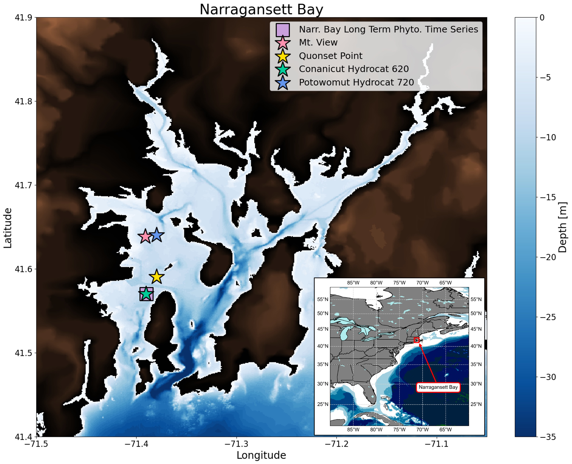
Figure 1. Map of sensor and sample collection sites in Narragansett Bay (NOAA, 1998). Sensor-measured pH measurements were first checked for spurious values and then verified against in situ samples. Conanicut Hydrocat (green star) and Quonset Point (yellow star) were compared to weekly samples collected from the Narragansett Bay Long Term Phytoplankton Time Series site (purple box). Potowomut Hydrocat (blue star) and Mt. View (pink star) were compared to monthly samples collected from the Potowomut site (blue star).

The Conanicut Hydrocat and Potowomut Hydrocat sensors are HydroCAT-EP (SeaBird) that measure pH, along with temperature, salinity, and DO, every 15 minutes approximately 1 meter below the surface, and were co-located with sensors measuring meteorological conditions (e.g. maximum precipitation, average wind speed, maximum gust wind speed, and air temperature) 2.4 meters above the surface every 10 minutes.

The sensors were deployed year-round and were recovered after periods of no longer than 3 months for maintenance, at which point the flow path and the conductivity cell are flushed with 1% Triton detergent followed by vigorous flushing with DI water. Following the cleaning, a zero conductivity check and a two point calibration are performed for conductivity. For pH, the probe was cleaned and a three point calibration was done with standards of pH 4, 7, and 10. Data from the Conanicut and Potowomut sensors were first subjected to a global range check to ensure that measurements were within the range of values measured across all marine environments using the dataset provided by OOI (NSF Ocean Observatories Initiative, 2018), followed by a local range test using data from the Narragansett Bay Long-Term Plankton Time Series data (https://web.uri.edu/gso/research/plankton/; see Section 2.2.2). The range suggested by the Narragansett Bay Long-Term Plankton Time Series, with only a weekly resolution, could be overly restrictive, so a ±0.1 variance was permitted, which encompassed most of the daily variability observed in the sensor data. This ensured that some high or low pH values, mostly associated with short-term variability, were not erroneously deemed spurious. The data was then despiked to remove spurious values, and subjected to a stuck value test, comparing each measurement with the 5 preceding measurements to ensure there were no repeated measurements indicating sensor error (Kelley and Richards, 2023).

The MV and QP sensors were YSI brand multi-parameter sondes (EXO V2 and 6-series-6600EDS, respectively) and maintained by the Narragansett Bay Fixed Station Monitoring Network (NBFSMN; RIDEM, 2020). Each sensor, located 1 m below the surface, measures pH, along with temperature, salinity, and DO, every 15 minutes and were deployed seasonally (spring to fall) and removed during winter months. These data were subject to quality assurance measures including verification of calibrations and consistency among multiple instruments, corrections for sensor drift and biases due to biofouling, removal of outliers, and interpolation across selected intervals of missing data, in accordance with the Rhode Island Department of Environmental Management’s (RIDEM) Quality Assurance Plan (RIDEM, 2020). Protocols for calibration, field maintenance, and quality assurance and quality control (QA/QC) procedures are consistent with National Estuarine Research Reserve System-Wide Monitoring Program standard operating procedures (Mensinger, 2019). Stations were serviced by swapping the deployed instruments with newly calibrated instruments on a 2-week interval. Calibrations and sensor drift corrections were verified through a three-point comparison: data from the retrieved sonde were compared to the newly calibrated sonde, as well as an independent profiling sonde, all at the deployment depth. Outliers and data errors were removed based on criteria set in the RIDEM Quality Assurance Project Plan (RIDEM, 2020). Gaps in coverage, affecting up to 6% of the record at an individual station in a given year, were filled by linear interpolation following protocols detailed in the Quality Assurance Project Plan (RIDEM, 2020).

The high temporal resolution of the time series enabled us to detect patterns of variability across multiple timescales. We used the Prophet forecasting model software (Taylor and Letham, 2018) to identify diurnal (i.e. daily) patterns. Other timescales of variability (e.g. monthly and seasonal) were identified using timemeans. The historical summertime (June, July, and August [JJA]) pH data for 2005 to 2019 from NBFSMN sites (QP and MV; Figure 1), in addition to the more recent data from the Conanicut and Potowomut sites for 2021 and 2022, were analyzed for multi-year trends. Unlike the recent (2022 - 2023) NBFSMN data, which were measured every 15 minutes, the historical (2005 - 2019) NBFSMN data from QP and MV were provided as daily means. The Conanicut and Potowomut data used in the historical analysis were processed as daily means in order to correspond with the historical NBFSMN data. The historical NBFSMN data were subject to quality assurance protocols previously outlined for the MV and QP sensors, as set forth by RI Department of Environmental Management, NBFSMN, and NERRS (RIDEM, 2020; Mensinger, 2019). We conducted change-point detection—with change-points indicating where the properties of the time series abruptly change—using the ruptures Python package (Truong et al., 2020). This analysis was applied to mean summertime pH and maximum daily summertime pH to identify carbonate system shifts in Narragansett Bay over the last two decades, especially in the wake of nutrient reductions to Narragansett Bay (RIDEM, 2016).

2.2.2 Discrete bottle samples

Discrete bottle samples were collected to verify the sensor data. Samples for the southern region of the bay (i.e. near QP and Conanicut buoy; see Figure 1) were collected weekly as part of the Narragansett Bay Long Term Phytoplankton Time Series (PLT), which is located just off the Conanicut buoy. The time series typically collects samples on Monday mornings at approximately 7:30am, barring weeks when inclement weather conditions delayed or canceled sampling. Samples for the northern region of the bay (i.e. Greenwich Bay near MV and Potowomut buoy), a region in which hypoxic events occur seasonally during the summer due to terrestrial nutrient inputs (Oviatt et al., 2017), were collected approximately once a month. After collection, samples were poisoned with 100 µM of saturated mercuric chloride solution and stored in the refrigerator until analysis for DIC and TA. DIC and TA were measured according to Dickson et al. (2007) using the Apollo SciTech Model AS-C6L Dissolved Inorganic Carbon Analyzer and the Apollo SciTech Model AS-ALK3 Total Alkalinity Titrator. Instruments were calibrated to Certified Reference Material (CRM) from Scripps Institute of Oceanography at room temperature (21 - 22°C). For DIC analysis, a sample of CRM was run prior to and at the end of sample analysis for quality control. TA analysis was calibrated to CRM, and either a sample of CRM or aged open ocean water was run at beginning of daily analysis and end of daily analysis for quality control. Lab-based measurements carry a ±0.2% uncertainty for alkalinity and ±0.1% uncertainty for DIC.

2.2.3 Quality assurance and control

First, we performed a gross range test on sensor data to eliminate unrealistic data (i.e. pH measurements less than 5 or greater than 10, or DO less than 1 mg L⁻¹) that indicate biofouling or other sensor malfunction. We then despiked the data by removing any data points that were more than 3 standard deviations greater or less than the sensor’s annual mean or any data points that were more than 1.5 standard deviations greater than or less than the sensor’s 24-hour moving mean.

Autonomous pH observations were compared to pH values calculated from DIC and TA in the discrete samples (see Section 2.3 for calculation). Periods of sensor data that diverged from bottle sample data with consistent, identifiable bias—for instance, a consistent underestimation or overestimation of pH by a value less than 0.1 pH unit or a dynamic bias less than 0.1 pH unit that changes with temperature or time—were corrected. In the case of QP, we corrected this by adjusting all the sensor data points by the mean difference between sensor pH and bottle pH, specifically lowering QP pH by 0.084 units. The Conanicut Hydrocat buoy overestimated pH in January-March 2023 when temperatures were lowest. We applied a more dynamic correction as a third order polynomial function of temperature, such that sensor pH was adjusted to be lower at colder temperatures. Figure 2 presents the corrected data from all four sensors with discrete bottle data. Conanicut Hydrocat and QP sensors were compared to PLT bottle samples, whereas Potowomut Hydrocat and MV sensors were compared to GB bottle samples.

Figure 2

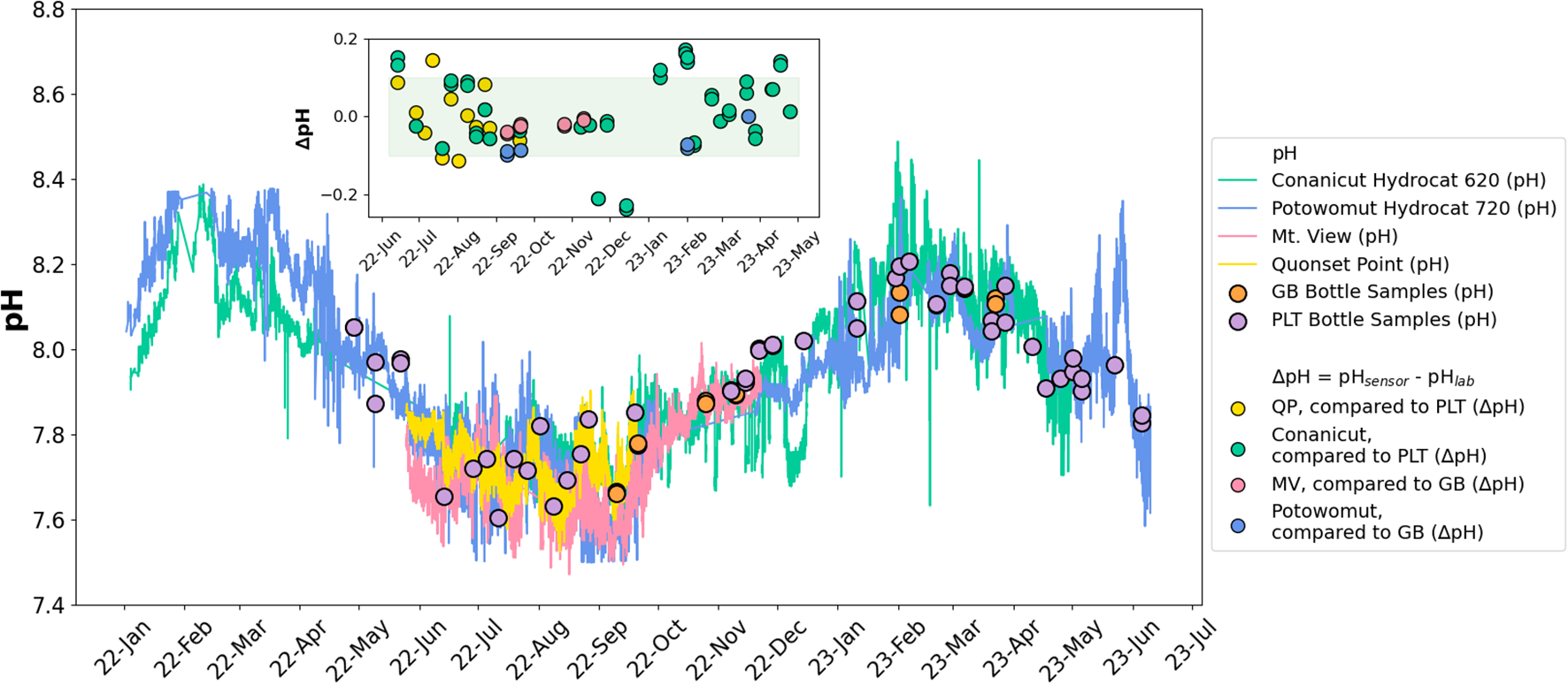
Figure 2. Outer: Time series of pH in Narragansett Bay. Sensors in the norther region of the Bay (i.e. Greenwich Bay) are Potowomut Hydrocat 720 (blue) and MV (pink) and correspond to GB bottle samples (oranges circles). Sensors in the southern region of the bay are Conanicut Hydrocat 620 (green) and QP (yellow) and correspond to Narragansett Bay Long Term Phytoplankton Time Series (PLT) bottle samples (purple circles). Inner: Differences between sensor-measured pH within 30 minutes of sampling time and in situ sample. Green bar represents uncertainty of the pH sensors.

2.3 Carbonate chemistry calculations

Solving the marine carbonate systems requires at least two known parameters from the following: DIC, TA, pH, and pCO₂. The autonomous monitoring system provided only one carbonate parameter: pH. However, a strong, linear relationship between salinity and alkalinity permitted a robust estimate of alkalinity for sufficiently high salinity values. Equation 3, as reported by Pimenta et al. (2023), describes the alkalinity-salinity relationship for Narragansett Bay, which is valid for mid- to high salinities found throughout most of Narragansett Bay (i.e. S ≥ 15). The data from this study fit well with this linear model. Using Equation 3, we estimated alkalinity from salinity (TA_S). Then, with salinity, temperature, pH, and TA_S, we determined the marine carbonate system—namely for DIC, hydrogen ion concentration ([H⁺]), pCO₂, and all associated errors —using PyCO2SYS (Humphreys et al., 2022). We used carbonate equilibrium constants from Lueker et al. (2000) and estimated total borate according to Uppström (1974).

$\begin{array}{ll}{\text{TA}}_{\text{mix}}=477.62+51.99*\text{S}& (3)\end{array}$

2.4 Air-sea CO₂ flux

Using pCO₂ calculated from pH and TA_S, hereafter referred to as $pC{O}_2^{calc}$, we solved for the ASF of carbon according to Equation 4 (Sarmiento and Gruber, 2006; Wanninkhof, 2014). For this, we assumed atmospheric pCO₂ to be 410 µatm (Lan et al., 2023). While the assumption of a constant atmospheric pCO₂ does neglect the seasonal variability in atmospheric pCO₂, this variability is much smaller than the observed seasonal variability in surface water pCO₂, which can change by several hundred ppm from winter to summer. We calculated solubility (K_solubility) using sensor-measured temperature and salinity according to Weiss (1974) and transfer velocity (K_t) according to Equation 5 (Wanninkhof, 2014) using sensor-measured 15 minute wind speed. Wind speed was measured at a height of 2.4 meters, but was adjusted to a height of 10 meters (for U₁₀), according to Atlas et al. (2011). Note that Sc refers to the Schimdt number.

$\begin{array}{ll}\varphi ={\text{K}}_{\text{t}}*{\text{K}}_{\text{solubility}}({\text{pCO}}_2^{\text{calc}}-{\text{pCO}}_2^{\text{air}})& (4)\end{array}$

$\begin{array}{ll}{\text{K}}_{\text{t}}=0.251\langle U_{10}^2\rangle {\frac{Sc}{660}}^{-0.5}& (5)\end{array}$

Notably, Equation 4 yields an ASF in units of µmolC m⁻² time−1; however, for our later Taylor series deconvolution analysis (described in Section 2.5), we required units of µmolC kg⁻¹ time−1. To achieve this, we normalized ASF by dividing by total water depth, which we considered to be an adequate estimate of the mixed layer depth in estuaries like Narragansett Bay that are either well-mixed or weakly stratified, and divided by density ρ. We calculated CO₂ ASF for each available time step (i.e. every 15 minutes) and, for a seasonal perspective, integrated that over one month, such that fluxes for every time-step were in units of µmolC kg⁻¹ month⁻¹. Over the course of a whole month, ASF should affect the full depth of the water column, as the CO₂ transfer velocity is generally around 2 m day⁻¹. For a daily perspective, we similarly integrated each 15 minute flux over 24 hours, such that fluxes for every time-step were in units of µmolC kg⁻¹ day⁻¹. While the typical CO₂ transfer velocity of 2 m day⁻¹ is not large enough to assume that ASF affects the full depth on daily time scales, using this daily analysis for periods of high wind, during which the CO₂ transfer velocity increases to as much as 10 m day⁻¹, can minimize any potential overestimations of ASF. The equation for ASF is shown in Equation 6, where i indicates each time-step over a given period τ, which, in the case of this analysis, is either 1 month or 1 day, and where H indicates the local height of the water (i.e. between 7 and 9 m, depending on location) and ρ indicates the in-situ density.

$\begin{array}{ll}{\text{DIC}}_{\text{ASF}}=\overline{\varphi }{|}_{\tau }=\frac{1}{\tau H}{\sum }_{n=1}^i{\text{K}}_{{\text{t}}_{\text{i}}}*{\text{K}}_{{\text{solubility}}_{\text{i}}}({\text{pCO}}_{2i}{}^{calc}-{\text{pCO}}_{2i}{}^{air})*\frac{\tau }{\rho }& (6)\end{array}$

2.5 pH driver analysis

In order to disentangle the various drivers of pH variability, we first considered pH change in terms of change of [H⁺], to avoid issues with the nonlinearities in the pH scale (Fassbender et al., 2021). We then employed a first order Taylor series deconvolution of drivers, based on Kwiatkowski and Orr (2018); Ma et al. (2023), and Cai et al. (2021), of either monthly [H⁺] variability for our seasonal analysis or daily [H⁺] variability for an analysis of an extreme weather event that occurred over the course of one week in December 2022. Similar use of Taylor series deconvolutions for the carbonate system were used by Wright-Fairbanks and Saba (2022); Pacella et al. (2024), and Rheuban et al. (2019). We identified seven potential drivers: temperature, salinity, the biological component of alkalinity and DIC from net metabolism, the mixing component of alkalinity and DIC primarily from tides, and the ASF of CO₂. The Taylor series deconvolution is given in Equation 7. We assumed any residual term implied by the Taylor series is small, as other processes contributing to [ΔH⁺] in Narragansett Bay, namely carbonate formation and dissolution, are minor. Note that the DIC_ASF term does not include Δ, since DIC_ASF already represents a flux over time.

$\begin{array}{ll}\begin{array}{c}\Delta [{\text{H}}^{+}]\approx [\frac{\partial [H^{+}]}{\partial T}\Delta \text{T}]+[\frac{\partial [H^{+}]}{\partial S}\Delta \text{S}]+{[[\frac{\partial [H^{+}]}{\partial TA}\Delta {\text{TA}}_{\text{bio}}]+[\frac{\partial [H^{+}]}{\partial DIC}\Delta {\text{DIC}}_{\text{bio}}]]}_{\text{bio}}\\ +{[[\frac{\partial [H^{+}]}{\partial TA}\Delta {\text{TA}}_{\text{mix}}]+[\frac{\partial [H^{+}]}{\partial DIC}\Delta {\text{DIC}}_{\text{mix}}]]}_{\text{mix}}+[\frac{\partial [H^{+}]}{\partial DIC}\Delta {\text{DIC}}_{\text{ASF}}]\end{array}& (7)\end{array}$

Using PyCO2SYS’s built-in functionality, we differentiated [H⁺] in terms of temperature and salinity (i.e. $\frac{\partial [H^{+}]}{\partial T}$ and $\frac{\partial [H^{+}]}{\partial S}$). Multiplying the partial derivatives by discretizations of temperature and salinity over time (i.e. $\Delta \text{T}$ and $\Delta \text{S}$) gave components of Δ[H+] for temperature and salinity (i.e. $\text{Δ}{[{\text{H}}^{+}]}_{\text{T}}$ and $\text{Δ}{[{\text{H}}^{+}]}_{\text{S}}$)

With total DIC calculated from pH and TAS, along with its uncertainty, we solved for the DIC components of Equation 7 and further broke DIC down into its mixing, ASF, and biological components (i.e. $\text{Δ}{[{\text{H}}^{+}]}_{{\text{DIC}}_{\text{ASF}}}$, $\text{Δ}{[{\text{H}}^{+}]}_{{\text{DIC}}_{\text{mix}}}$, and $\text{Δ}{[{\text{H}}^{+}]}_{{\text{DIC}}_{\text{bio}}}$). First we isolated the effect of mixing on DIC by using the relationship between DIC and salinity in Narragansett Bay found by Pimenta et al. (2023), given in Equation 8.

$\begin{array}{ll}{\text{ΔDIC}}_{\text{mix}}=397.65+50.59*\text{ΔS}& (8)\end{array}$

We isolated the ASF component of DIC according to Equation 6, as previously discussed in Section 2.4 (Sarmiento and Gruber, 2006; Wanninkhof, 2014), and normalized it to a mixed layer depth equal to local water column depth—7 meters in the mid-bay near Conanicut and QP sensors, and 9 meters slightly northward near the Potowomut and MV sensors. Note that this assumes Narragansett Bay is well-mixed year-round. This is a reasonable assumption given that the central and southern regions of Narragansett Bay tend to be well-mixed or weakly stratified (Pilson, 1985; Oviatt et al., 2002). However, this may lead to slight overestimation when Narragansett Bay is weakly stratified.

The biological component of DIC—that is, the net amount of DIC metabolically consumed and produced by the local biological community of bacteria, phytoplankton, zooplankton, etc.—was assumed to be the remainder of DIC, after accounting for mixing and ASF (Equation 9). Each component of DIC, except for ASF, which already describes a change in carbon over time, was then discretely differentiated over time, by month for the seasonal analysis and by day for the analysis of a week-long weather event.

$\begin{array}{ll}{\text{ΔDIC}}_{\text{bio}}=\text{ΔDIC}-{\text{DIC}}_{\text{ASF}}-{\text{ΔDIC}}_{\text{mix}}& (9)\end{array}$

The mixing and biological components of TA were separated, first, by employing Equation 3 (Pimenta et al., 2023) to solve for the mixing component. The biological component—the net amount of alkalinity metabolically consumed and produced by the local biological community—was solved by multiplying DIC_bio by the Redfield ratio (i.e. $\frac{-16}{107}$; see Equation 10; Anderson & Sarmiento, 1994; Sarmiento and Gruber, 2006). We assumed carbonate production and dissolution were negligible, because of the strong linear relationship between alkalinity and salinity. Finally, the sum of the effects of mixing on DIC and total alkalinity represent a net mixing component $\text{Δ}{[{\text{H}}^{+}]}_{\text{mix}}$; likewise, the sum of the biological effects on both DIC and alkalinity represent the net impact of NEM as $\text{Δ}{[{\text{H}}^{+}]}_{\text{bio}}$.

$\begin{array}{ll}{\text{ΔTA}}_{\text{bio}}=\frac{-16}{107}*{\text{ΔDIC}}_{\text{bio}}& (10)\end{array}$

2.6 Net ecosystem metabolism

In order to independently verify our calculations for DIC_bio (Equation 9), we estimated the net metabolic production of carbon of the whole ecosystem from the diurnal cycle of DO. A time series dataset of DO, as measured by the Conanicut Hydrocat and Potowomut Hydrocat sensors, was used to estimate net ecosystem metabolism (NEM), the balance between primary production and respiration integrated over the whole ecosystem (Caffrey et al., 2014). We used a simplified one-dimensional mass balance method as described in Caffrey et al. (2014) and Oviatt et al. (2017). The change of DO ($\frac{dDO}{dt}$) is the sum of the air-sea interface exchange (J), biological production (P), and respiration (R), as shown in Equation 11. Notably, this formulation makes the a priori assumption that in relatively well-mixed and shallow estuaries, the mixing of oxygen will be negligible compared to oxygen’s metabolic and gas exchange contributions.

$\begin{array}{ll}\frac{dDO}{dt}=\text{P}-\text{R}+\text{J}& (11)\end{array}$

As NEM is the net effect of production and respiration, we rearranged Equation 11 as Equation 12. This revealed that, not only can NEM be calculated from gross production and respiration, but can also be calculated using the total change in DO minus oxygen air-sea gas exchange.

$\begin{array}{ll}\text{NEM}=\text{P}-\text{R}=\frac{dDO}{dt}-\text{J}& (12)\end{array}$

The daily change of DO was defined as the change between dawns, which accounts for seasonally varying day lengths. Air-sea oxygen flux (J) was estimated from an empirical transfer coefficient (K; Equation 13) and oxygen saturation deficit (SD; Equation 14), both based on Kremer et al. (2003). The calculation of K required wind speed at 10 meters (U₁₀). We obtained wind speed at a height of 2.4 meters from sensors collocated with Conanicut Hydrocat and Potowomut Hydrocat sensors at 10 minute intervals. Wind speed data was then normalized to 10 meters following Atlas et al. (2011), as described in Section 2.4.

$\begin{array}{ll}\text{K}=0.55e^{0.15*{\text{U}}_{10}}& (13)\end{array}$

$\begin{array}{ll}\text{SD}={\text{pO}}_2^{\text{atm}}*\frac{D{O}_{sat}-D{O}_{obs}}{D{O}_{sat}}, {\text{pO}}_2^{\text{atm}}=0.209 \text{atm}& (14)\end{array}$

The contribution of collapsing bubbles on air-sea exchange of oxygen cannot be ignored. Bubble injection terms for small, fully collapsing bubbles (F_c) and large, partially collapsing bubbles (F_p), as described in Bushinsky and Emerson (2018), were added to calibrate the bubble impact on air-sea oxygen flux. Thus, the total air-sea exchange of oxygen is given in Equation 15.

$\begin{array}{ll}\text{J}=\text{K}*\text{SD}+{\text{F}}_{\text{c}}+{\text{F}}_{\text{p}}& (15)\end{array}$

We calculated NEM for days with at least 22 hours of DO and wind data; fluxes were extrapolated for any gaps shorter than 2 hours without notable error. Since Narragansett Bay tends to be well-mixed or only weakly stratified (Pilson, 1985), we took mixed layer depth as the total depth of the local water column, as we did in the calculation of ASF and DIC_bio (Section 2.4). This assumption could potentially overestimate NEM during periods in which Narragansett Bay is weakly stratified, rather than well-mixed. However, the choice ensured consistency between our oxygen-based calculation of NEM and DIC_bio. NEM was then integrated over longer time periods (e.g. months) and converted from oxygen units to carbon units using a ratio of 150 units of oxygen to 106 units of carbon (Anderson, 1995), enabling us to independently verify our calculations for DIC_bio.

3 Results

Figure 2 shows the full pH time series across all sensors after QA/QC. Autonomous pH corresponds closely with in situ samples. The mean difference between QP and PLT discrete samples was 0.00002, between Conanicut Hydrocat and PLT discrete samples was 0.008, between MV and GB discrete samples was -0.02, and between Potowomut Hydrocat and GB discrete samples was -0.06. The mean difference overall across all sites is -0.002. The more northern sites (MV and Potowomut) likely have higher pH discrepancies when compared to discrete data due to less frequent samples being taken at the GB site. All the discrepancies are less than the ±0.1 uncertainty introduced by the pH sensors (SeaBird Scientific, 2023). A distinct signal of diurnal and seasonal pH variability was observed in all four time series. In the following sections, we analyze these patterns of variability and their drivers.

3.1 Diurnal cycle

Figure 3 shows the isolated diurnal cycles of temperature, DO, and pH for each season, averaged across our four pH sensors in local, Eastern Standard Time, plus 1 standard deviations (shaded bands), with all other timescales of variability longer than a day being removed. The diurnal cycle is shown as anomalies about the daily mean. Temperature (Figure 3A) on average decreased from the daily mean by 0.21 ± 0.11°C by 3:22AM and increased from the daily mean by 0.23 ± 0.11°C by 10:58AM. DO (Figure 3B) decreased from the daily mean by 0.20 ± 0.19 mg L⁻¹ by 2:39AM and increased from the daily mean by 0.24 ± 0.26 mg L⁻¹ by 12:54PM. On average, pH (Figure 3C) decreased from the daily mean by 0.02 ± 0.02 by 2:17AM—over an hour before the daily temperature minimum and less than half an hour before the daily DO minimum. pH then increased from the daily mean by 0.02 ± 0.02 by 1:08PM—over 2 hours after the daily temperature maximum and less than half an hour after the daily DO maximum. The diurnal cycle of pH, which had a range of 0.05 to 0.1 units, tracked closely with both temperature and DO. A linear correlation between daily temperature variation and daily pH variation yielded an R² value of 0.47, and a linear correlation between daily variations in DO and pH yielded an R² value of 0.83.

Figure 3

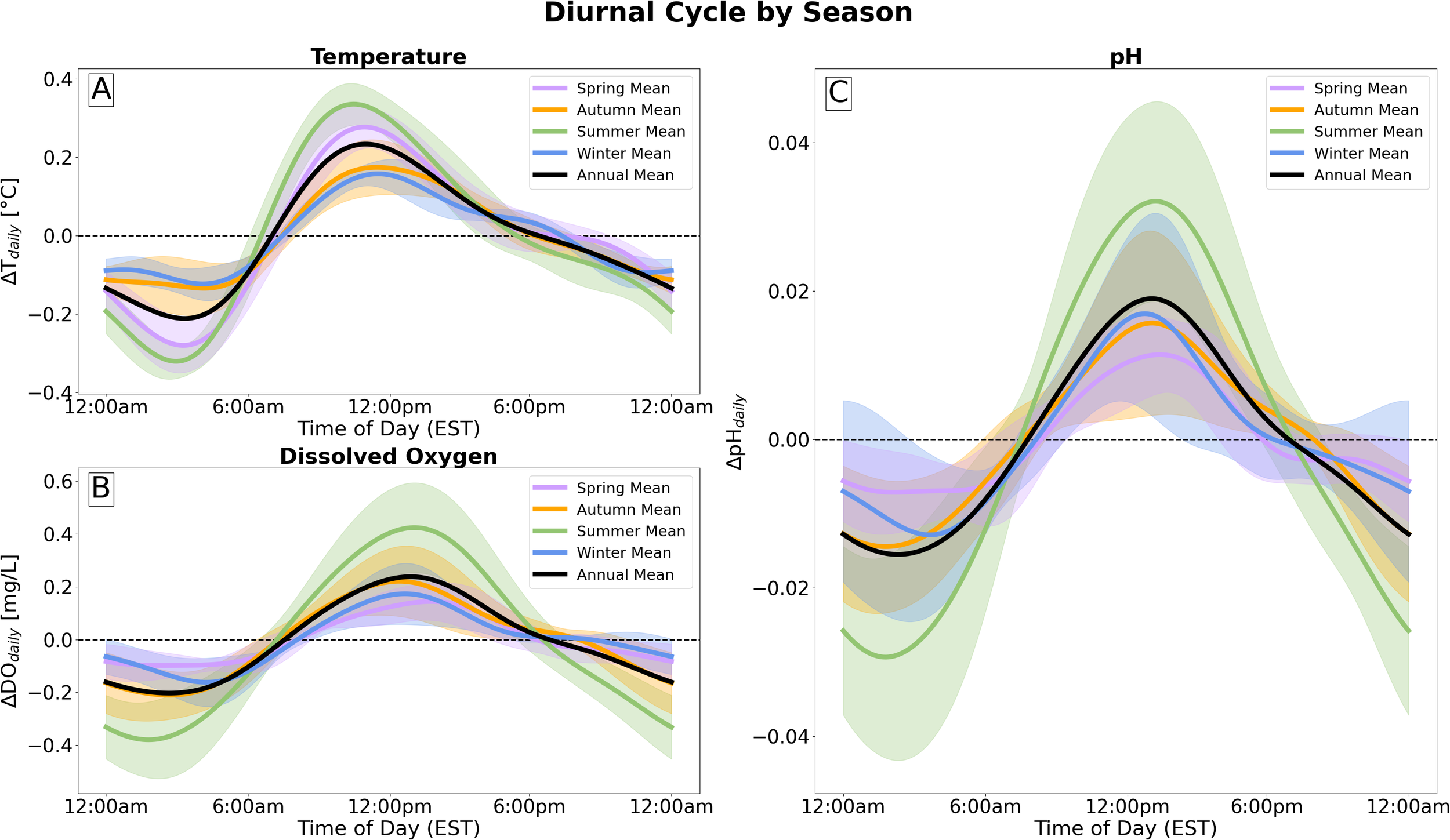
Figure 3. Diurnal cycle of (A) temperature, (B) dissolved oxygen, and (C) pH, calculated using Prophet (Taylor and Letham, 2018), for each season, averaged across all sensors. Time is given as local Eastern Standard Time (EST). Shaded bands represent 1 standard deviation.

The diurnal cycles of temperature, DO, and pH varied across seasons in amplitude. The timing of daily temperature and DO minima and maxima remained roughly consistent across seasons, varying by approximately an hour. Summer experienced the largest range of daily temperature and DO variability, 0.66 ± 0.04°C and 0.79 ± 0.13 mg L⁻¹, respectively. Following these patterns, timing of pH daily minima and maxima remained approximately the same across all seasons, and pH was most variable in summer, ranging by 0.06 ± 0.01 pH units throughout the day. pH was least variable in spring, ranging by 0.02 ± 0.01 pH units.

3.2 Seasonal cycle

Monthly pH from all four sites in Narragansett Bay revealed a distinct seasonal cycle (Figure 4C). pH was highest in the wintertime, reaching a maximum in February ($\overline{{\text{pH}}_{\text{Feb}}}=8.2\pm 0.1$). pH was lowest in the summertime, reaching a minimum in August ($\overline{{\text{pH}}_{\text{Aug}}}=7.7\pm 0.1$). The seasonality of pH corresponded with the seasonality of DO (Figure 4B), yet the inverse of temperature (Figure 4A). These seasonalities in Narragansett Bay found in this study agree with Pimenta et al. (2023) based on monthly survey from January 2017 to December 2019.

Figure 4

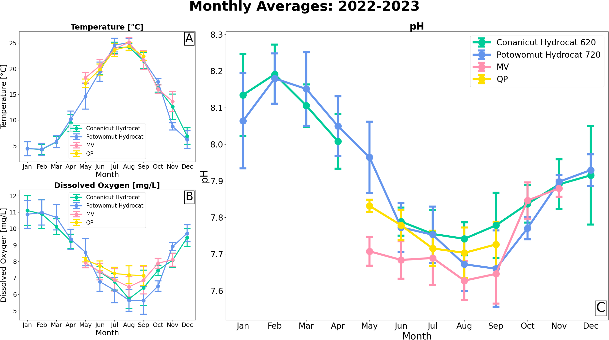
Figure 4. Monthly averages of (A) temperature, (B) dissolved oxygen, and (C) pH with 1 standard error from all 4 sensors.

3.3 Net ecosystem metabolism

Figure 5A compares monthly NEM with monthly DIC_bio. NEM was calculated from the diurnal cycle of oxygen (Equation 12) and converted to units of mmolC m⁻³ month⁻¹. Note that positive NEM values, when in carbon units, indicate heterotrophy. DIC_bio was calculated from the DIC mass balance (Equation 9) in order to independently verify the calculation of DIC_bio used in the Taylor series deconvolution (see Equation 7 and Section 3.4). The entirety of NEM and DIC_bio is presented in Figures 5B, C.

Figure 5

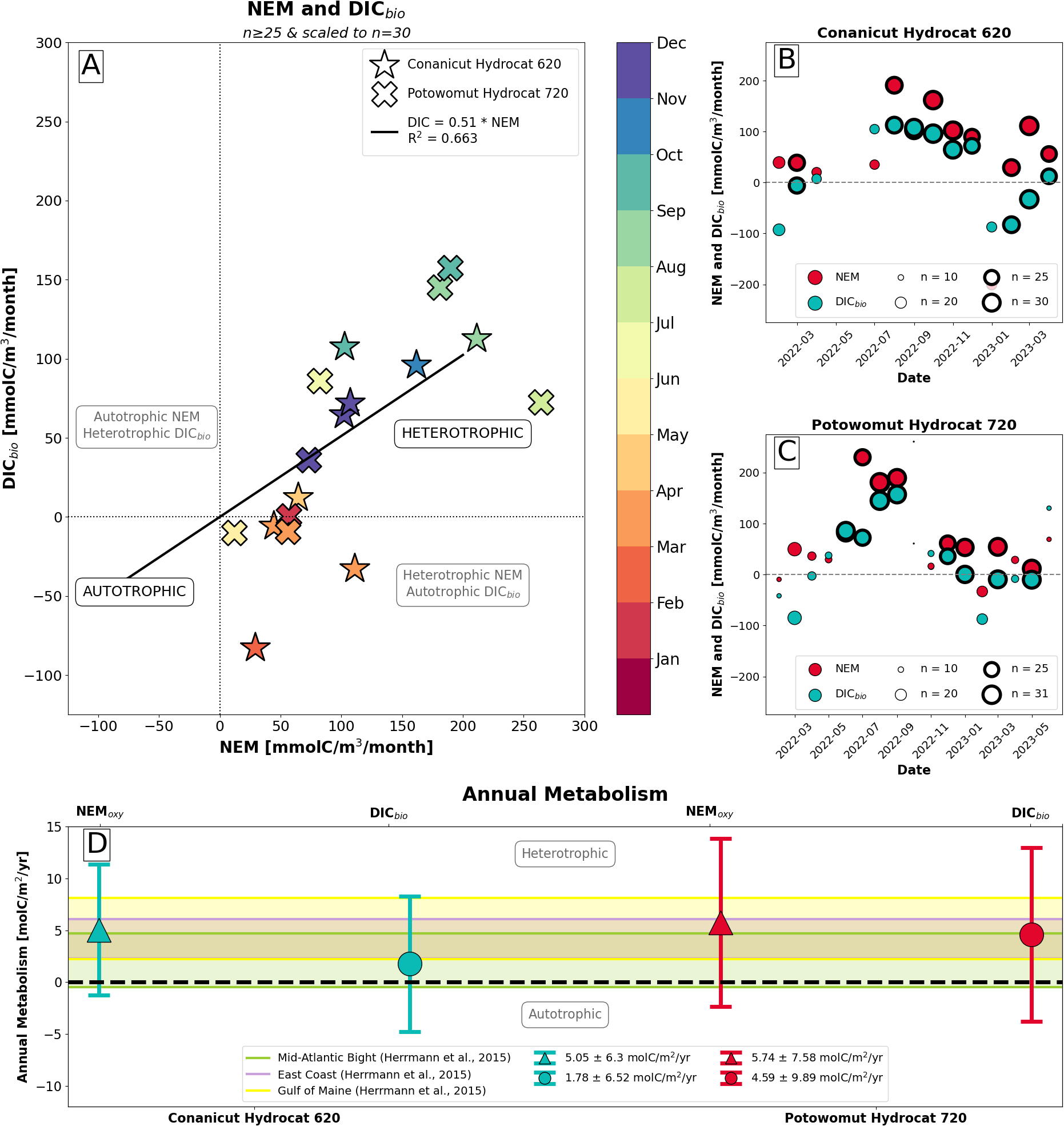
Figure 5. Monthly net ecosystem metabolism. (A) Comparison of monthly net ecosystem metabolism, calculated from dissolved oxygen (Equation 12) and converted to units of mmolC m⁻³ month⁻¹, with monthly DIC_bio (Equation 9). Recall that positive NEM values, when in carbon units, indicate heterotropy. Stars indicate values from Conanicut Hydrocat 620. X-marks indicate values from Potowomut Hydrocat 720. Points are colored by month of the year. Only months with a minimum of 25 days of data are included, and values are scaled to 30 days. A linear trendline intersecting the origin relating DIC_bio and NEM has a slope of 0.51 (R² = 0.663). (B, C) All monthly values of DIC_bio (teal) and NEM (red) for Conanicut Hydrocat 620 (B) and Potowomut Hydrocat 720 (C) prior to scaling to 30 days, where point size corresponds to number of days with data in each month. Bold points have at least 25 days of data and were included in (A, D) Annual metabolism at Conanicut Hydrocat 620 (teal) and Potowomut Hydrocat 720 (red), calculated using oxygen-based NEM (triangles) and DIC_bio (circles). Annual metabolisms from Herrmann et al. (2015) for the Mid-Atlantic Bight, East Coast, and Gulf of Main—shown as green, purple, and yellow shaded bars, respectively—are provided for reference.

We fitted the data with a linear model intersecting the origin, which had a slope of 0.51 (R² = 0.663). This indicated that for every 1 mmolC m⁻³ month⁻¹ increase in NEM, DIC_bio increased by 0.51 mmolC m⁻³ month⁻¹. Since we expected the relationship between NEM in carbon units and DIC_bio to be one-to-one, the 0.51 slope suggests DIC_bio underestimated NEM and [H⁺] changes resulting from biological activities, or vice versa.

While oxygen-based calculations of NEM in the winter did not reflect wintertime autotrophy, we considered DIC_bio to be more accurate in these circumstances, given the existing, extensive research supporting a wintertime phytoplankton bloom in Narragansett Bay (Oviatt et al., 2002, 2017; Baumann and Smith, 2018), as well large wintertime chlorophyll concentrations (Figure 6B). However, the overall consistency between oxygen-based NEM and DIC_bio increased confidence in the accuracy and reliability of the DIC_bio calculations. In this study we used DIC_bio to represent a more conservative NEM estimation to maintain alignment with other processes that impact the DIC pool.

Figure 6

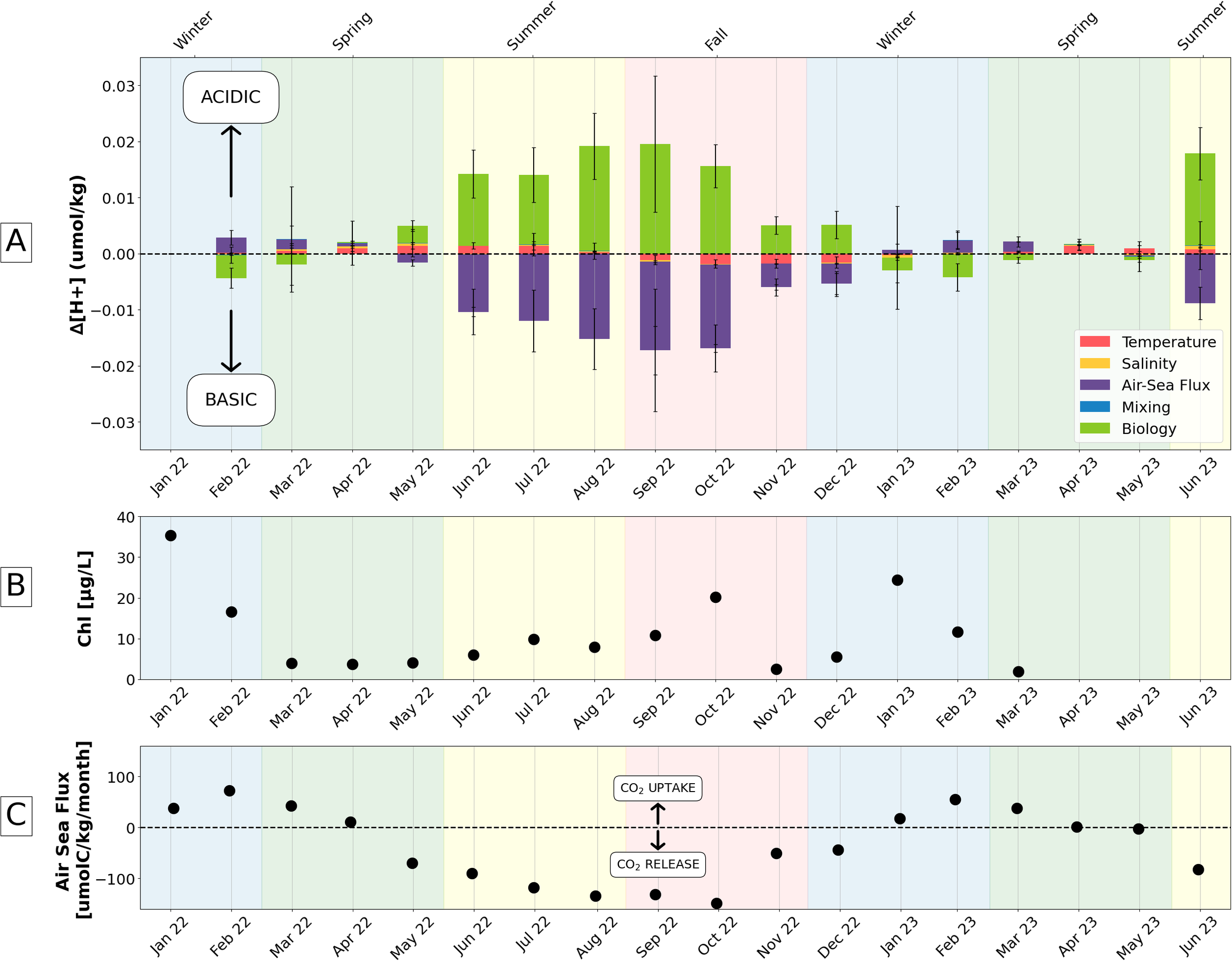
Figure 6. Drivers of seasonal [H⁺] variability (A) Results from first order Taylor series deconvolution (Equation 7), averaged across all sensors, describing drivers of hydrogen ion concentration change on monthly timescales. Increases in hydrogen ion concentration correspond with lower pH and acidification. (B) Mean monthly chlorophyll concentration from the Narragansett Bay Long Term Phytoplankton Time Series. (C) Air-sea flux of carbon dioxide as carbon, calculated according to Equations 4 and 5 (Wanninkhof, 2014). The positive direction indicates marine carbon dioxide uptake and vice versa.

By integrating the monthly NEM and DIC_bio values over the whole year we obtained the annual metabolic carbon budget (Figure 5D). At Conanicut Hydrocat, the ecological community produced 5.05 ± 6.3 molC m⁻² yr⁻¹, when calculated from NEM, and 1.78 ± 6.52 molC m⁻² yr⁻¹, when calculated from DIC_bio. At Potowomut Hydrocat, the ecological community produced 5.74 ± 7.58 molC m⁻² yr⁻¹, when calculated from NEM, and 4.59 ± 9.89 molC m⁻² yr⁻¹, when calculated from DIC_bio. Overall, this indicated that Narragansett Bay on annual timescales is heterotrophic, with some months of autotrophy during the wintertime phytoplankton bloom. The annual metabolic carbon budgets in Narragansett Bay largely agreed with the heterotrophic annual metabolic carbon budgets in the Mid-Atlantic Bight, Gulf of Maine, and along the entire US East Coast (Herrmann et al., 2015), though Narragansett Bay’s budget demonstrated higher variability than these sites, which can be expected of an estuary.

3.4 Seasonal pH drivers

The analysis of the monthly drivers of pH variability through a first order Taylor series deconvolution (Equation 7) demonstrated a similar seasonality to what is described in Section 3.2 and Figure 4. The results of this deconvolution, averaged across all sensors, are shown in Figure 6A, along with monthly averaged observed chlorophyll concentration from the Narragansett Bay Long Term Phytoplankton Time Series (Figure 6B) and ASF, calculated according to Equations 4 and 5 (Figure 6C).

Wintertime pH in December, January, and February, as shown through change in [H⁺] (Figure 6A), is dominated by biological/metabolic processes (i.e. photosynthesis and respiration) and CO₂ ASF. Wintertime biological activity, as part of Narragansett Bay’s winter-spring phytoplankton bloom (Oviatt et al., 2002), decreased [H⁺] (i.e. higher pH) and accounted for an average of 67% of wintertime [ΔH⁺] decrease. Further, the wintertime uptake of CO₂ through ASF (Figure 6C), which had a maximum rate of 72.68 µmolC kg⁻¹ month⁻¹ in February 2022, increased [H⁺] (i.e. lower pH), in opposition to the effect of biological activities; wintertime ASF accounted for 100% of the [ΔH⁺] increase. Temperature had a small, slightly basifying effect in the winter, depending on the extent of cooling each month, representing on 23% of winter [ΔH⁺] decrease. The combined effect of biological processes and ASF in the wintertime varied month to month, but generally was slightly basifying.

Spring (i.e. March, April, and May) was a transitional period in Narragansett Bay. Narragansett Bay gradually switched from a CO₂ sink to source and released CO₂ at a rate of 69.95 µmolC kg⁻¹ month⁻¹ by May, partially offsetting acidification from biology and temperature. CO₂ uptake had a slightly weaker effect than in winter, representing 27% of the increase in [H⁺] toward more acidic conditions. Metabolic processes, which became increasingly more dominated by organic matter respiration throughout the spring, remained the one of the largest drivers of [ΔH⁺], accounting for 100% of the increase in [H⁺], toward more acidic conditions, unlike winter. Warming temperatures were responsible for 61% of springtime [H⁺] increase. The combined springtime effect of all the drivers was acidifying.

When pH was lowest in the summer (i.e. June, July, and August), biology contributed most to the observed increase in [H⁺] through net heterotrophy, an observation reinforced by persistently low chlorophyll concentrations leading into and lasting throughout the summer (Figure 6B). Net heterotrophy comprised 93% of [H⁺] increase and was decisively acidifying in the summer. This coincided with the acidifying effect of warming temperatures in the summer, which represented 6% of [H⁺] increase, though this temperature effect abated by the end of summer. The CO₂ outgassing in the summer (Figure 6C), with an seasonal average rate of 106.2 µmolC kg⁻¹ month⁻¹ responsible for 100% of the [H⁺] decrease, reduced CO₂ accumulation and had a basifying effect that nearly offset the thermodynamically- and biologically-induced acidification. The combined effect of all the drivers in the summer was acidifying.

By fall (i.e. September, October, and November), chlorophyll levels modestly increased to values greater than 10 µg L⁻¹ (Figure 6B), indicating a slight increase in primary production. The metabolism was, however, still net heterotrophic, though slightly more weakly so, accounting for 100% of [H⁺] increase and decreasing pH. Cooling beginning in September, in addition to ongoing CO₂ release (Figure 6C), opposed the slightly acidifying effect of declining heterotrophy in the fall. Respectively, cooling and CO₂ release accounted for 12% and 87% of [H⁺] decrease. However, the effect of ASF diminished by the end of fall, as CO₂ release weakened from 148.99 µmolC kg⁻¹ month⁻¹ in October to 51.02 ± 0.8 µmolC kg⁻¹ month⁻¹ in November. The combined effect of all the drivers in the fall was weakly basifying, leading into Narragansett Bay’s more basic wintertime regime.

3.5 Winter storm pH drivers

In addition to our seasonal analysis, we specifically focused on a week-long winter storm that occurred from December 19th through 26th, 2022. Over this period, wind speeds increased to as much as 17.6 m s⁻¹ (39.4 ^mph) on December 23 and water temperatures decreased by as much as 3.9°C from December 19 to December 26, with most of that decline occurring on or after December 24. Precipitation was moderate—totaling approximately 50 mm over the course of the week and occurring primarily on December 22 and December 23.

Over the course of the week, pH increased at both sites by 0.045 pH units (Figure 7B). The lowest average hourly pH occurred on the morning of December 19 at both sites: 8.01 ± 0.01 at the Conanicut Hydrocat buoy and 7.93 ± 0.01 at the Potowomut Hydrocat buoy. The highest average hourly pH occurred later in the week: 8.1 ± 0.01 at the Conanicut Hydrocat buoy on the night of December 24 and 8.02 ± 0.01 at the Potowomut Hydrocat buoy in the evening of December 26. During this event, pH anomalies were weakly and negatively correlated with temperature anomalies (r = -0.36) and were moderately and positively correlated with dissolved oxygen (r = 0.45).

Figure 7

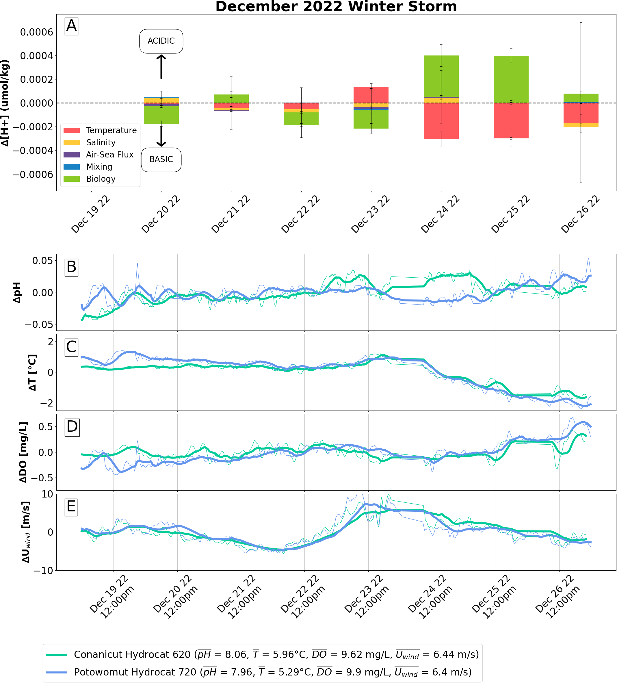
Figure 7. Drivers of [H⁺] variability during a December 2022 storm. (A) Results from first order Taylor series deconvolution (Equation 7), averaged across two sensors with available wintertime data (Conanicut Hydrocat 620 and Potowomut Hydrocat 720), describing the drivers of hydrogen ion concentration change on a daily timescale during a winter storm occurring from December 20, 2022 to December 26, 2022. A decrease in hydrogen ion concentration equates to higher pH and basification, and vice versa. Time series of (B) pH (C) temperature, (D) dissolved oxygen, and (E) wind speeds are shown as anomalies. Thin lines are 1 hour moving means. Thick lines are 6 hour moving means, to reduce noise. Anomalies are calculated as moving mean minus total mean.

Using the first order Taylor series deconvolution of [H⁺] (Equation 7) to analyze the drivers of pH change (Figure 7A), we found that the major contributor to changes in [H⁺] during this winter storm was increasing biological respiration, despite the net autotrophy at the beginning of this storm (i.e. prior to December 24). Toward the beginning of the week (December 20 to December 23, excluding December 21 when metabolism is briefly heterotrophic), an autotrophic metabolism dominated [H⁺] change, tending to decrease [H⁺] (i.e. higher pH). The average change in [H⁺] due to biological metabolism from December 20 to December 23 (excluding December 21) was 0.00014 ± 0.00005 µmol kg⁻¹, corresponding to an average of 71% of [H⁺] decrease.

By the end of the week (December 24 to December 26), biological respiration increased. The metabolism became more heterotrophic and began to increase $[{\text{H}}^{+}]$ ($\overline{{\text{ΔH}}_{\text{bio}}}{|}_{\text{Dec \hspace{0.33em}}24}^{\text{Dec \hspace{0.33em}}26}=0.00027\pm 0.00011\mu \text{mol kg}-1$). On average, biological processes were responsible for 94% of the increase [H⁺] over this period.

Other drivers, primarily temperature and salinity, only partially offset the effects of biological processes. In the beginning of the week (i.e. prior to December 24), gradually cooling temperatures and decreasing salinity due to precipitation tended to compound the basifying effects of photosynthesis, except for on December 23 when temperatures briefly increase ($\overline{{\text{ΔH}}_{\text{T}}}{|}_{\text{Dec \hspace{0.33em}}19}^{\text{Dec \hspace{0.33em}}22}$ = 0.000036 ± 0.000002 $\mu \text{mol} {\text{kg}}^{-1}$; $\overline{{\text{ΔH}}_{\text{S}}}{|}_{\text{Dec \hspace{0.33em}}19}^{\text{Dec \hspace{0.33em}}23}$ = 0.000011 ± 0.000002 $\mu \text{mol} {\text{kg}}^{-1}$). This resulted in a net basifying effect through the beginning of the week, excluding December 21 (when net change in [H⁺] was 0 µmol kg⁻¹). However, by the end of the week (i.e. December 24 to December 26), when the metabolism became more heterotrophic, cooling temperatures offset the increased [H+] from biological activity through $[{\text{H}}^{+}]$ decrease ($\overline{{\text{ΔH}}_{\text{T}}}{|}_{\text{Dec \hspace{0.33em}}24}^{\text{Dec \hspace{0.33em}}26}$ = 0.00025 ± 0.00011 $\mu \text{mol} {\text{kg}}^{-1}$); the net effect then became weakly acidifying. The week, on the whole, demonstrated a decrease in [H⁺]/pH increase, with a dampened trend toward higher pH values late in the week.

3.6 Long term pH trends

Figure 8 shows long-term summertime pH trends from the MV and QP sites. Mean daily summertime pH (Figure 8A) decreased at both MV and QP and showed change points at in 2015-2016, nearly a decade after nutrient reductions first began, with decreases of 0.08 pH units and 0.04 pH units, respectively. Maximum daily mean pH (Figure 8B) similarly decreased at both MV and QP. MV showed a change point in 2016, associated with a 0.13 unit decrease in maximum daily pH; QP showed a change point in 2015, associated with a 0.11 unit decrease in maximum daily pH. As such, both sites experienced systematic decreases in surface pH 3 to 4 years after the successful implementation of nitrogen loading reductions, where both sites became slightly more acidic in the surface.

Figure 8

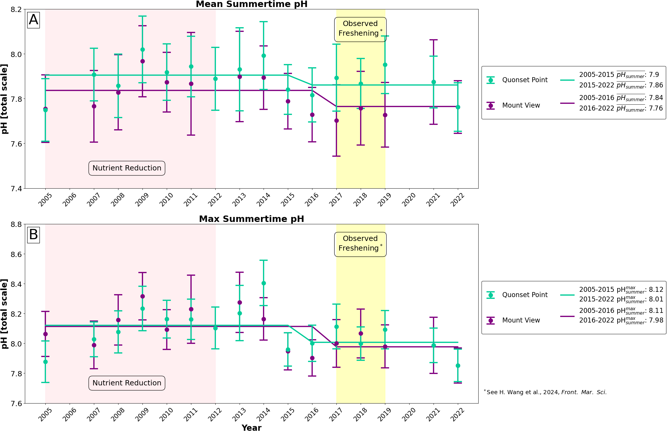
Figure 8. Long-term pH summer (JJA) pH time series for NBFSMN sites, Quonset Point (green) and Mnt. View (purple). All historical data (2005-2019) was subjected to the QA/QC protocol outlined in RIDEM (2020); additionally, 2021 and 2022 data were further verified against in situ samples. (A) Mean summertime pH and (B) maximum summertime daily mean pH value were are analyzed for change points using ruptures (Truong et al., 2020). The period of nutrient reductions from 2005 to 2012 is highlighted in pink. A period of freshening, observed by Wang et al. (2024), from 2017 to 2019 is highlighted in yellow.

4 Discussion

4.1 Diurnal cycle

The close correspondence of daily DO variability and pH variability (Figure 3) was the first evidence that pH variability in Narragansett Bay has been largely controlled by biological production, underscoring the importance of biological activity on this estuarine carbonate system. Specifically, pH decreased at night when light availability limits photosynthesis and increased during the day when photosynthesis occurs. This broadly agrees with the results from Wang et al. (2018), who found that in the Duplin River (GA, USA) DIC tended to increase (corresponding to a pH decrease) through the night while DO decreased, indicating respiration dominated the metabolism outside of daylight hours. Secondarily, pH positively correlated with temperature, such that daily pH increased as daily temperature increased. This was contrary to the typical thermal response of pH to temperature, in which increasing temperatures lower pH. We suggest, in this circumstance, temperature was merely an artifact of light availability. This strong, positive correlation between pH and DO on diurnal timescales has been observed in multiple NERRS habitats (Baumann and Smith, 2018). Note that pH and DO daily variability are highest in summer, represented by the largest difference in daily minima and maxima (Figure 3). We suggest that this high variability was due to summer’s weak carbonate buffer capacity resulting from the strong heterotrophic state (Figure 5), but could also be due to increased rates of biological production and respiration with warmer temperatures.

4.2 Drivers of monthly and seasonal carbonate variability

The large control of biology through its metabolism on carbonate variability in Narragansett Bay extends to monthly and seasonal timescales as well (Wang et al., 2018; Baumann and Smith, 2018; Rheuban et al., 2019; Wallace et al., 2014). As suggested by Figure 4 and explicitly shown in Figure 6, biological activity was the dominant driver of [H⁺] concentration change on monthly timescales, but was closely followed by CO₂ ASF. Temperature change from month to month was a smaller, yet still notable driver. The effect of temperature was more intuitive on monthly to seasonal time scales than on daily timescales, as it follows thermodynamic effects—warmer temperatures correspond with more acidic conditions.

In the following we discuss the three main drivers of pH variability on monthly to seasonal timescales—biological activity (i.e. the net metabolism), ASF, and temperature. However, we must note the other drivers included in our analysis: mixing and salinity. In the deconvolution of pH drivers (Equation 7; Figure 6), the effects of DIC and alkalinity mixing have been summed for a total effect of mixing. While the respective contributions of DIC and alkalinity mixing varied from month to month, they compensated for one another such that the total mixing effect was near zero and never accounted for more than 2% of the change in [H⁺]. Salinity also had a relatively small effect on monthly timescales (i.e. an average of 1.58% of the monthly change in [H⁺]), but notably may have had a larger effect on shorter time scales that can temporally resolve rain or drought events.

4.2.1 Biology & metabolism

Our comparison of oxygen-based NEM and DIC_bio showed that our calculations for DIC_bio were reasonably accurate, based on the oxygen budget, though may slightly underestimate heterotrophy. The underestimation was reasonable given the much slower CO₂ ASF compared to oxygen (Sarmiento and Gruber, 2006). Generally, oxygen measurements are more sensitive to short-term changes in respiration and photosynthesis, while the DIC pool reflects the monthly average change. Regardless, we contend that biological acidification during summer and fall, when Narragansett Bay is typically heterotrophic, may have be stronger than reported. However, this discrepancy has not changed the leading role community metabolism has in driving seasonal acidification; if anything, it underscored its intensity.

Throughout the year in Narragansett Bay, biological activity was the strongest driver of [H⁺] change, based on calculations of DIC_bio. By mid-winter around January, biological activity, which has become increasingly dominated by photosynthesis through winter, begun to decrease [H⁺] in Narragansett Bay (shown by green bars in Figure 6), making the water column more basic. This period coincided with the onset of Narragansett Bay’s winter phytoplankton bloom in January and February, when a more autotrophic net metabolism consumed CO₂ and released DO (see Figure 4B).

After the decline of the winter-spring phytoplankton bloom, primary production abated due to nutrient limitation (Oviatt et al., 2002), and the net community metabolism becames heterotrophic through the summer. This was confirmed by low concentrations of DO (i.e. below saturation) in summer and fall (Figure 4B). The enhanced respiration, in turn, elevated pCO₂ and [H⁺], peaking during the summer months. However, by fall, hetetrotrophy weakened, resulting in decreased biologically-induced acidification that was overcome by the effect of other drivers, and the net change of [H⁺] change was negative (i.e. weakly basifying).

4.2.2 Air sea flux

Estuaries functioning as annual CO₂ sources is well-documented in some of the world’s largest estuary systems, like Chesapeake Bay and the Pearl River Estuary (Liu et al., 2022; Herrmann et al., 2020), though these estuaries are seasonal CO₂ sinks during bloom periods. As Liu et al. (2022) suggest, CO₂ ASF, at least in part, is a response to an estuary’s NEM, since NEM is one of the most influential sources/sinks of carbon in estuaries. We have found a similar dynamic in Narragansett Bay, where ASF was the second largest driver of [ΔH⁺]. Through summer and fall and even into the beginning of winter, CO₂ outgassing worked to oppose the acidifying effect of biology’s net heterotrophy. Because of warm waters decreasing CO₂ solubility and increased respiration providing a seasonal source of dissolved CO₂, pCO₂ was higher than atmospheric levels, often in excess of 500 µatm in the summer. The loss of excess CO₂ to the atmosphere, which averaged 87.23 µmolC kg⁻¹ month⁻¹ from May to December, mitigated acidification. The magnitude of summertime [ΔH⁺] due to CO₂ outgassing was almost large enough to offset the effect of biological processes, yet it fell slightly short because CO₂ ASF is slower than metabolic processes.

By mid-winter, Narragansett Bay switched from a CO₂ source to CO₂ sink. From December 2022 to February 2023, ASF in Narragansett Bay changes from a release of 44.06 µmolC kg⁻¹ month⁻¹ to an uptake of 55.39 µmolC kg⁻¹ month⁻¹. The combination of greater CO₂ solubility in cold, winter waters and greater air-sea interface turbulence from characteristically stronger wintertime wind increased uptake of CO₂ beginning in January through much of the spring. The addition of CO₂ to the water column from the atmosphere subsequently released [H⁺]. Through winter, uptake of CO₂ was not large enough to overcome the basifying effect of net photosynthesis —the inverse of summer’s and fall’s ASF effect. Thus, year-round, ASF was the second largest driver of [ΔH⁺], tending to oppose the seasonal effect of biological activities. However, the consistent near-equal opposition by ASF to biological activities may be somewhat overestimated due to (A) ΔDIC_bio being calculated from DIC_ASF and ΔDIC_mix (see Equation 9) and thus containing a small residual term and (B) the assumption of the mixed layer being equal to the water column.

4.2.3 Temperature

The third largest driver of [H⁺] change in Narragansett Bay was temperature. From a thermodynamics perspective, warming decreases CO₂ solubility, while also increasing the carbonate system’s dissociation reactions. Specifically with warming, H₂CO₃ more readily dissociates into $HC{O}_3^{-}$, resulting in the release of a hydrogen ion. $HC{O}_3^{-}$ even more readily dissociates into $C{O}_3^{2-}$, resulting in the release of an additional hydrogen ion. Decreased CO₂ solubility under warming may work against the thermodynamic effect on $HC{O}_3^{-}$ and $C{O}_3^{2-}$, but CO₂ gas exchange is slow to equilibrate pCO₂ with the atmosphere, while chemical equilibration is nearly instantaneous (Cai et al., 2011; Millero, 1995). Thus, the immediate effect of warming/cooling observed in Narragansett Bay was increased/decreased acidity, and temperature’s effect of hydrogen ion concentration followed annual patterns of cooling and warming.

4.3 December storm drivers

The community metabolism was the main contributor to the change in [H⁺] during the 2022 winter storm, followed closely by temperature (Figure 7). During the beginning of the week, from December 20 through December 23, biological activity tended to basify the water column as the storm reaches its climax (i.e. a short warm front with increasing wind speeds and brief precipitation on December 23). This suggests a more autotrophic metabolism during the beginning of the week, likely enabled by water column mixing bringing nutrients and primary producers into the euphotic zone. However, the metabolism became more heterotrophic by the end of the week. This is similar to the response to Chesapeake Bay to Hurricane Isabel in the summer of 2003. High winds during Hurricane Isabel drove water column mixing that increased primary production. However, the mixing of ammonium to the surface enabled a diatom bloom that more than offset enhanced primary production and led to a 0.2 to 0.3 unit decrease in surface pH (Hall et al., 2023). Decreases in pH following storms may also have been due to enhanced runoff from precipitation delivering more nutrients, DIC, and organic matter to the estuary, as was observed in Texas’s Baffin Bay, Nueces Estuary, Guadalupe Estuary, and Lavaca-Colorado Estuary (Montagna et al., 2018), or from the mixing of bottom water organic matter. While a pulse of nutrients may have initially spurred primary production, the delivery of DIC and organic matter to respire ultimately resulted in more acidic conditions.

Temperature was the second most significant driver, initially causing an increase in [H⁺] before quickly leading to a decrease, contributing to 12.84% of the total [H⁺] changes. In contrast to its impact on monthly timescales (Figure 6), ASF played a minimal role during this event due to the slow exchange rate. Additionally, unlike the monthly timescale, salinity exerted a moderate influence during the storm, due to precipitation. Overall, the December 2022 storm illustrated that while biology predominantly drove the carbonate system over short timescales as well as longer timescales, temperature and, to some extent, salinity, became more significant factors.

4.4 Long term trends under nutrient reduction

Nitrogen loading reductions since 2005 have successfully alleviated bottom water hypoxia and increased bottom water pH (Codiga et al., 2022, 2009; Oviatt et al., 2017, 2022; Wang et al., 2024), which has beneficial for the overall health of the bay’s ecosystem. Our previous discussions have confirmed the dominant role of biological processes in driving pH changes from weekly to monthly timescales. Therefore, nutrient reduction should naturally reduce surface pH, alongside the observed increases in bottom DO and pH conditions.

Interestingly, Wang et al. (2024) found no significant changes in the bay-mean annual average surface pH, despite the combined effects of anthropogenic CO₂ dissolution and declining surface primary production, both of which typically lower pH. This lack of significant change was attributed to strong natural variability. However, the data treatment in Wang et al. (2024) (i.e. annual bay-wide average) may have smoothed out the signal of nutrient reduction when its effects are most pronounced. To address this, we adopted two indices—the seasonal maximum pH and the seasonal mean—from the summer months, when nutrient reductions have been most successful in reducing hypoxia.

Using these two new approaches, we found that the maximum summertime pH, directly linked to primary productivity, has decreased since nitrogen reduction efforts began (Figure 8B). This provided strong evidence of the impact that strict nutrient reduction has on primary productivity and, subsequently, on surface pH, especially when the pH is naturally low in the summer. However, the decreasing trend was less pronounced for the mean summertime pH, which showed only a modest decline around 2015 compared to the maximum pH. This discrepancy may have been due to the freshening of Narragansett Bay observed between 2017 and 2019. As reported by Wang et al. (2024), bay-wide salinity during this period was 3 PSU lower than average, resulting from increased precipitation and river discharge, which may have increased pH by approximately 0.05 units. In other words, natural variability makes it difficult to discern the changes in mean summer pH caused by nutrient reduction.

Notably, Narragansett Bay’s response to nutrient reductions (i.e. the decreases in mean and maximum summertime pH) appeared to occur 3 to 4 years after the 50% nitrogen load reductions were achieved in 2012 (RIDEM, 2016; Oviatt et al., 2022; Codiga et al., 2022). With change points detected in 2015 at QP and 2016 at MV (Figure 8), a decade after nitrogen reductions were first implemented and 3 to 4 years after nitrogen reduction goals were first met, we observed that Narragansett Bay’s carbonate system has a delayed response—and a response that is likely still developing—to nutrient management. Previous studies have found that estuaries with reduced external nutrient loading can have a sluggish biogeochemical response as a result of a “legacy” of nutrients remaining in the sediment, to be released and recycled for years to come (Testa et al., 2022; Cormier et al., 2023; Pitkänen et al., 2001). This is particularly relevant in Narrganasett Bay, as summertime benthic nutrient regeneration in the Providence River Estuary and upper bay supply 5–30% of the phytoplankton nitrogen demand (Fulweiler et al., 2010). This is to say, the delayed and likely evolving biogeochemical response of Narragansett Bay to reduced external nitrogen loads is not unexpected and underscores the importance of internal nutrient loading in management decisions.

Narragansett Bay demonstrates the complicated biogeochemical response to watershed management and nutrient reduction efforts. On one hand, nutrient reductions can increase pH and DO concentrations in bottom water, while also improving water clarity and light penetration, which may further increase bottom pH and DO through increased production. On the other hand, nutrient reductions may modestly decrease surface production and surface pH, particularly in the summer when pH is naturally low. Indeed, nutrient management shifts the balance between surface and bottom water productivity. As nutrient reductions continue to be implemented, more research is needed to fully understand how these changes will affect ecosystem services in the whole water column, such as fisheries, aquaculture, and carbon sequestration, as well as the resilience of the ecosystem to future stressors like climate change and ocean acidification.

5 Conclusion

Using four high temporal resolution pH time series, we found that like many other estuaries, pH in Narragansett Bay fluctuates both daily and seasonally, following general patterns of estuarine productivity. pH tended to be higher during periods of peak production, such as daytime or during a winter-spring algal bloom. While the impact of temperature on surface pH was relatively minor, especially on longer timescales (i.e. seasonal to annual), and the impact of salinity even more minor, nutrient reduction played a significant role in driving surface pH changes on interannual timescales, especially in estuarine environments. Looking ahead, future warming may have a minor effect on pH. However, anthropogenic forcings like nutrient reduction are likely to be a more crucial factor in shaping estuarine surface pH changes alongside the uptake of anthropogenic CO₂. This study captures the effects of nutrient reduction on surface pH during the summer months when these interventions are most impactful, providing a clearer picture of the ongoing carbonate chemistry changes in the context of climate change and active human management.

Data availability statement

Data sets generated as part of this study, specifically discrete carbonate data from the Narragansett Bay Long Term Phytoplankton Time Series site and Greenwich Bay and autonomous pH data from Conanicut, Potowomut, Quonset Point, and Mount View, have been made available on BCO-DMO (i.e. https://doi.org/10.26008/1912/bco-dmo.961940.1 and https://doi.org/10.26008/1912/bco-dmo.961920.1). Preexisting datasets from Narragansett Bay leveraged by this study can be found at the following links: https://web.uri.edu/gso/research/plankton/data/ and https://web.uri.edu/gso/research/marine-ecosystems-research-laboratory/datasets/. Additional software written as part of this study, specifically for the NEM calculation and the Taylor series deconvolution, can be found on Github at https://github.com/abby-baskind/NarrBay. The GitHub repository includes copies of datasets published to BCO-DMO.

Author contributions

AB: Conceptualization, Data curation, Formal analysis, Investigation, Methodology, Project administration, Software, Supervision, Validation, Visualization, Writing – original draft, Writing – review & editing. GA: Formal analysis, Investigation, Writing – original draft, Writing – review & editing. KG: Data curation, Resources, Validation, Writing – review & editing. HS: Data curation, Resources, Validation, Writing – review & editing. SG: Methodology, Software, Validation, Writing – review & editing. AD: Conceptualization, Funding acquisition, Resources, Supervision, Validation, Writing – review & editing. HW: Conceptualization, Funding acquisition, Methodology, Project administration, Resources, Supervision, Validation, Writing – review & editing.

Funding

The author(s) declare that financial support was received for the research and/or publication of this article. This work is graciously supported by National Science Foundation (NSF) funding through OCE-2241991.

Acknowledgments

Discrete bottle data for this study has been collected in collaboration with the Narragansett Bay Long Term Phytoplankton Time Series, directed by Tatiana Rynearson and assisted by Bryan Plankenhorn (2022-2023) and John Selby (2023-present), aboard R/V Cap’n Bert, captained by Stephen Barber. Autonomous pH data were collected in collaboration with URI’s Marine Ecosystems Research Lab (MERL), directed by Candace Oviatt, and the Narragansett Bay Fixed Station Monitoring Network (NBFSMN), managed by Heather Stoffel. Additionally, URI’s Summer Undergraduate Research Fellowship in Oceanography (SURFO) supported contributions by summer intern Georgia Ahumada. The team behind this study would specifically like to thank lab manager Cathy Cipolla, undergraduate lab assistant Joseph Sudano, and Lieutenant Junior Grade Paul Slife.

Conflict of interest

The authors declare that the research was conducted in the absence of any commercial or financial relationships that could be construed as a potential conflict of interest.

Generative AI statement

The author(s) declare that no Generative AI was used in the creation of this manuscript.

Publisher’s note

All claims expressed in this article are solely those of the authors and do not necessarily represent those of their affiliated organizations, or those of the publisher, the editors and the reviewers. Any product that may be evaluated in this article, or claim that may be made by its manufacturer, is not guaranteed or endorsed by the publisher.

References

Anderson L. A. (1995). On the hydrogen and oxygen content of marine phytoplankton. Deep sea Res. Part I: Oceanographic Res. papers 42, 1675–1680. doi: 10.1016/0967-0637(95)00072-E

Crossref Full Text | Google Scholar

Anderson L. A. and Sarmiento J. L. (1994). Redfield ratios of remineralization determined by nutrient data analysis. Global biogeochemical cycles 8 (1), 65–80. doi: 10.1029/93gb03318

Crossref Full Text | Google Scholar

Atlas R., Hoffman R. N., Ardizzone J., Leidner S. M., Jusem J. C., Smith D. K., et al. (2011). Supplement: A cross-calibrated, multiplatform ocean surface wind velocity product for meteorological and oceanographic applications. Bull. Am. Meteorological Soc. 92, ES4–ES8. doi: 10.1175/2010BAMS2946.1

Crossref Full Text | Google Scholar

Baumann H. and Smith E. M. (2018). Quantifying metabolically driven pH and oxygen fluctuations in US nearshore habitats at diel to interannual time scales. Estuaries Coasts 41, 1102–1117. doi: 10.1007/s12237-017-0321-3

Crossref Full Text | Google Scholar

Beaufort L., Probert I., de Garidel-Thoron T., Bendif E. M., Ruiz-Pino D., Metzl N., et al. (2011). Sensitivity of coccolithophores to carbonate chemistry and ocean acidification. Nature 476, 80–83. doi: 10.1038/nature10295

PubMed Abstract | Crossref Full Text | Google Scholar

Breitburg D., Levin L. A., Oschlies A., Grégoire M., Chavez F. P., Conley D. J., et al. (2018). Declining oxygen in the global ocean and coastal waters. Science 359, eaam7240. doi: 10.1126/science.aam7240

PubMed Abstract | Crossref Full Text | Google Scholar

Bushinsky S. M. and Emerson S. R. (2018). Biological and physical controls on the oxygen cycle in the Kuroshio Extension from an array of profiling floats. Deep Sea Res. Part I: Oceanographic Res. Papers 141, 51–70. doi: 10.1016/j.dsr.2018.09.005

Crossref Full Text | Google Scholar

Caffrey J. M., Murrell M. C., Amacker K. S., Harper J. W., Phipps S., and Woodrey M. S. (2014). Seasonal and inter-annual patterns in primary production, respiration, and net ecosystem metabolism in three estuaries in the northeast Gulf of Mexico. Estuaries Coasts 37, 222–241. doi: 10.1007/s12237-013-9701-5

Crossref Full Text | Google Scholar

Cai W.-J., Feely R. A., Testa J. M., Li M., Evans W., Alin S. R., et al. (2021). Natural and anthropogenic drivers of acidification in large estuaries. Annu. Rev. Marine Sci. 13, 23–55. doi: 10.1146/annurev-marine-010419-011004

PubMed Abstract | Crossref Full Text | Google Scholar

Cai W.-J., Hu X., Huang W.-J., Murrell M. C., Lehrter J. C., Lohrenz S. E., et al. (2011). Acidification of subsurface coastal waters enhanced by eutrophication. Nat. Geosci. 4, 766–770. doi: 10.1038/ngeo1297

Crossref Full Text | Google Scholar

Cai W.-J., Huang W.-J., Luther G. W. III, Pierrot D., Li M., Testa J., et al. (2017). Redox reactions and weak buffering capacity lead to acidification in the Chesapeake Bay. Nat. Commun. 8, 369. doi: 10.1038/s41467-017-00417-7

PubMed Abstract | Crossref Full Text | Google Scholar

Chintala M. M., Ayvazian S. G., Boothman W., Cicchetti G., Coiro L., Copeland J., et al. (2015). Trend analysis of stressors and ecological responses, particularly nutrients, in the Narragansett Bay Watershed (Narragansett, RI: Narragansett Bay Estuary Program).

Google Scholar

Codiga D. L., Stoffel H. E., Deacutis C. F., Kiernan S., and Oviatt C. A. (2009). Narragansett Bay hypoxic event characteristics based on fixed-site monitoring network time series: intermittency, geographic distribution, spatial synchronicity, and interannual variability. Estuaries coasts 32, 621–641. doi: 10.1007/s12237-009-9165-9

Crossref Full Text | Google Scholar

Codiga D. L., Stoffel H. E., Oviatt C. A., and Schmidt C. E. (2022). Managed nitrogen load decrease reduces chlorophyll and hypoxia in warming temperate urban estuary. Front. Marine Sci. 9, 930347. doi: 10.3389/fmars.2022.930347

Crossref Full Text | Google Scholar

Cormier J. M., Coffin M. R., Pater C. C., Knysh K. M., Gilmour R. F. Jr., Guyondet T., et al. (2023). Internal nutrients dominate load and drive hypoxia in a eutrophic estuary. Environ. Monitoring Assess. 195, 1211. doi: 10.1007/s10661-023-11621-y

PubMed Abstract | Crossref Full Text | Google Scholar

Da F., Friedrichs M. A., St-Laurent P., Shadwick E. H., Najjar R. G., and Hinson K. E. (2021). Mechanisms driving decadal changes in the carbonate system of a coastal plain estuary. J. Geophysical Research: Oceans 126, e2021JC017239. doi: 10.1029/2021JC017239

Crossref Full Text | Google Scholar

Dickson A. G., Sabine C. L., and Christian J. R. (2007). Guide to best practices for ocean CO2 measurements (North Pacific Marine Science Organization).

Google Scholar

Doney S. C., Busch D. S., Cooley S. R., and Kroeker K. J. (2020). The impacts of ocean acidification on marine ecosystems and reliant human communities. Annu. Rev. Environ. Resour. 45, 83–112. doi: 10.1146/annurev-environ-012320-083019

Crossref Full Text | Google Scholar

Doney S. C., Fabry V. J., Feely R. A., and Kleypas J. A. (2009). Ocean acidification: the other CO2 problem. Annu. Rev. marine Sci. 1, 169–192. doi: 10.1146/annurev.marine.010908.163834

PubMed Abstract | Crossref Full Text | Google Scholar

Esbaugh A. J. (2018). Physiological implications of ocean acidification for marine fish: emerging patterns and new insights. J. Comp. Physiol. B 188, 1–13. doi: 10.1007/s00360-017-1105-6

PubMed Abstract | Crossref Full Text | Google Scholar

Fassbender A. J., Orr J. C., and Dickson A. G. (2021). Technical note: Interpreting pH changes. Biogeosciences 18, 1407–1415. doi: 10.5194/bg-18-1407-2021

Crossref Full Text | Google Scholar

Feely R. A., Jiang L.-Q., Wanninkhof R., Carter B. R., Alin S. R., Bednaršek N., et al. (2023). Acidification of the global surface ocean. Oceanography 36, 120–129. doi: 10.5670/oceanog.2023.222

Crossref Full Text | Google Scholar

Friedlingstein P., Jones M. W., O’sullivan M., Andrew R. M., Bakker D. C., Hauck J., et al. (2022). Global carbon budget 2021. Earth System Sci. Data 14, 1917–2005. doi: 10.5194/essd-14-1917-2022

Crossref Full Text | Google Scholar

Fulweiler R. W., Nixon S. W., and Buckley B. A. (2010). Spatial and temporal variability of benthic oxygen demand and nutrient regeneration in an anthropogenically impacted New England estuary. Estuaries Coasts 33, 1377–1390. doi: 10.1007/s12237-009-9260-y

Crossref Full Text | Google Scholar

Hall N., Testa J., Li M., and Paerl H. (2023). Assessing drivers of estuarine pH: A comparative analysis of the continental USA’s two largest estuaries. Limnology Oceanography 68, 2227–2244. doi: 10.1002/lno.v68.10

Crossref Full Text | Google Scholar

Hall-Spencer J. M. and Harvey B. P. (2019). Ocean acidification impacts on coastal ecosystem services due to habitat degradation. Emerging Topics Life Sci. 3, 197–206. doi: 10.1042/ETLS20180117

PubMed Abstract | Crossref Full Text | Google Scholar

Herrmann M., Najjar R. G., Da F., Friedman J. R., Friedrichs M. A., Goldberger S., et al. (2020). Challenges in quantifying air-water carbon dioxide flux using estuarine water quality data: Case study for Chesapeake Bay. J. Geophysical Research: Oceans 125, e2019JC015610. doi: 10.1029/2019JC015610

PubMed Abstract | Crossref Full Text | Google Scholar

Herrmann M., Najjar R. G., Kemp W. M., Alexander R. B., Boyer E. W., Cai W.-J., et al. (2015). Net ecosystem production and organic carbon balance of US East Coast estuaries: A synthesis approach. Global Biogeochemical Cycles 29, 96–111. doi: 10.1002/2013GB004736

Crossref Full Text | Google Scholar

Hu X. and Cai W.-J. (2013). Estuarine acidification and minimum buffer zone—a conceptual study. Geophysical Res. Lett. 40, 5176–5181. doi: 10.1002/grl.v40.19

Crossref Full Text | Google Scholar

Hu X., Li Q., Huang W.-J., Chen B., Cai W.-J., Rabalais N. N., et al. (2017). Effects of eutrophication and benthic respiration on water column carbonate chemistry in a traditional hypoxic zone in the Northern Gulf of Mexico. Marine Chem. 194, 33–42. doi: 10.1016/j.marchem.2017.04.004

Crossref Full Text | Google Scholar

Humphreys M. P., Lewis E. R., Sharp J. D., and Pierrot D. (2022). PyCO2SYS v1. 8: marine carbonate system calculations in Python. Geoscientific Model Dev. 15, 15–43. doi: 10.5194/gmd-15-15-2022

Crossref Full Text | Google Scholar

Hunt C. W., Salisbury J. E., and Vandemark D. (2022). Controls on buffering and coastal acidification in a temperate estuary. Limnology Oceanography 67, 1328–1342. doi: 10.1002/lno.12085

Crossref Full Text | Google Scholar

Irby I. D., Friedrichs M. A., Da F., and Hinson K. E. (2018). The competing impacts of climate change and nutrient reductions on dissolved oxygen in Chesapeake Bay. Biogeosciences 15, 2649–2668. doi: 10.5194/bg-15-2649-2018

Crossref Full Text | Google Scholar

Jellison B. M. and Gaylord B. (2019). Shifts in seawater chemistry disrupt trophic links within a simple shoreline food web. Oecologia 190, 955–967. doi: 10.1007/s00442-019-04459-0

PubMed Abstract | Crossref Full Text | Google Scholar

Jiang L.-Q., Carter B. R., Feely R. A., Lauvset S. K., and Olsen A. (2019). Surface ocean pH and buffer capacity: past, present and future. Sci. Rep. 9, 18624. doi: 10.1038/s41598-019-55039-4

PubMed Abstract | Crossref Full Text | Google Scholar

Jiang Z.-P., Qin C., Pan Y., Le C., Rabalais N., Turner R. E., et al. (2024). Multi-decadal coastal acidification in the northern Gulf of Mexico driven by climate change and eutrophication. Geophysical Res. Lett. 51, e2023GL106300. doi: 10.1029/2023GL106300

Crossref Full Text | Google Scholar

Kelley D. and Richards C. (2023). oce: Analysis of Oceanographic Data, R package version 1.8-2.

Google Scholar

Kremer J. N., Reischauer A., and D’Avanzo C. (2003). Estuary-specific variation in the air-water gas exchange coefficient for oxygen. Estuaries 26, 829–836. doi: 10.1007/BF02803341

Crossref Full Text | Google Scholar

Kroeker K. J., Kordas R. L., Crim R. N., and Singh G. G. (2010). Meta-analysis reveals negative yet variable effects of ocean acidification on marine organisms. Ecol. Lett. 13, 1419–1434. doi: 10.1111/j.1461-0248.2010.01518.x

PubMed Abstract | Crossref Full Text | Google Scholar

Kwiatkowski L. and Orr J. C. (2018). Diverging seasonal extremes for ocean acidification during the twenty-first century. Nat. Climate Change 8, 141–145. doi: 10.1038/s41558-017-0054-0

Crossref Full Text | Google Scholar

Lan X., Tans P., and Thoning K. (2023). Trends in globally-averaged CO2 determined from NOAA global monitoring laboratory measurements. Version 2023-11. doi: 10.15138/9N0H-ZH07

Crossref Full Text | Google Scholar

Liu S., Gao Q., Wu J., Xie Y., Yang Q., Wang R., et al. (2022). Spatial distribution and influencing mechanism of CO2, N2O and CH4 in the Pearl River Estuary in summer. Sci. Total Environ. 846, 157381. doi: 10.1016/j.scitotenv.2022.157381

PubMed Abstract | Crossref Full Text | Google Scholar

Lowe A. T., Bos J., and Ruesink J. (2019). Ecosystem metabolism drives ph variability and modulates long-term ocean acidification in the Northeast Pacific coastal ocean. Sci. Rep. 9, 963. doi: 10.1038/s41598-018-37764-4

PubMed Abstract | Crossref Full Text | Google Scholar

Lueker T. J., Dickson A. G., and Keeling C. D. (2000). Ocean pCO2 calculated from dissolved inorganic carbon, alkalinity, and equations for K1 and K2: validation based on laboratory measurements of CO2 in gas and seawater at equilibrium. Marine Chem. 70, 105–119. doi: 10.1016/S0304-4203(00)00022-0

Crossref Full Text | Google Scholar

Ma D., Gregor L., and Gruber N. (2023). Four decades of trends and drivers of global surface ocean acidification. Global Biogeochemical Cycles 37, e2023GB007765. doi: 10.1029/2023GB007765

Crossref Full Text | Google Scholar

Mensinger M. (2019). National Estuarine Research Reserve System-Wide Monitoring Program (Georgetown, SC: NOAA National Estuarine Research Reserve System).

Google Scholar

Millero F. J. (1995). Thermodynamics of the carbon dioxide system in the oceans. Geochimica Cosmochimica Acta 59, 661–677. doi: 10.1016/0016-7037(94)00354-O

Crossref Full Text | Google Scholar

Mollica N. R., Guo W., Cohen A. L., Huang K.-F., Foster G. L., Donald H. K., et al. (2018). Ocean acidification affects coral growth by reducing skeletal density. Proc. Natl. Acad. Sci. 115, 1754–1759. doi: 10.1073/pnas.1712806115

PubMed Abstract | Crossref Full Text | Google Scholar

Montagna P. A., Hu X., Palmer T. A., and Wetz M. (2018). Effect of hydrological variability on the biogeochemistry of estuaries across a regional climatic gradient. Limnology Oceanography 63, 2465–2478. doi: 10.1002/lno.10953

Crossref Full Text | Google Scholar

Narita D., Rehdanz K., and Tol R. S. (2012). Economic costs of ocean acidification: a look into the impacts on global shellfish production. Climatic Change 113, 1049–1063. doi: 10.1007/s10584-011-0383-3

Crossref Full Text | Google Scholar

Nixon S. W., Buckley B. A., Granger S. L., Harris L. A., Oczkowski A. J., Fulweiler R. W., et al. (2008). “Nitrogen and phosphorus inputs to Narragansett Bay: past, present, and future,” in Science for ecosystem-based management: Narragansett Bay in the 21st century (New York: Springer), 101–175.

Google Scholar

NOAA (1998). Narragansett Bay, RI (M020) bathymetric digital elevation model (30 meter resolution) derived from source hydrographic survey soundings collected by NOAA (Silver Springs, MD: National Centers for Environmental Information).

Google Scholar

NSF Ocean Observatories Initiative (2018). Data product specification for pH of seawater (Washington DC: NSF Ocean Observatories Initiative).

Google Scholar

Orr J. C., Fabry V. J., Aumont O., Bopp L., Doney S. C., Feely R. A., et al. (2005). Anthropogenic ocean acidification over the twenty-first century and its impact on calcifying organisms. Nature 437, 681–686. doi: 10.1038/nature04095

PubMed Abstract | Crossref Full Text | Google Scholar

Oviatt C., Keller A., and Reed L. (2002). Annual primary production in Narragansett Bay with no bay-wide winter–spring phytoplankton bloom. Estuarine Coastal Shelf Sci. 54, 1013–1026. doi: 10.1006/ecss.2001.0872

Crossref Full Text | Google Scholar

Oviatt C., Smith L., Krumholz J., Coupland C., Stoffel H., Keller A., et al. (2017). Managed nutrient reduction impacts on nutrient concentrations, water clarity, primary production, and hypoxia in a north temperate estuary. Estuarine Coastal Shelf Sci. 199, 25–34. doi: 10.1016/j.ecss.2017.09.026

Crossref Full Text | Google Scholar

Oviatt C., Stoffel H., Huizenga K., Reed L., Codiga D., and Fields L. (2022). A tale of two spring blooms in a northeast estuary of the USA: how storms impact nutrients, multiple trophic levels and hypoxia. Hydrobiologia 849, 1131–1148. doi: 10.1007/s10750-021-04768-7

Crossref Full Text | Google Scholar

Pacella S. R., Brown C. A., Kaldy J. E., Labiosa R. G., Hales B., Mochon Collura T. C., et al. (2024). Quantifying the combined impacts of anthropogenic CO2 emissions and watershed alteration on estuary acidification at biologically-relevant time scales: a case study from Tillamook Bay, OR, USA. Front. Marine Sci. 11, 1293955. doi: 10.3389/fmars.2024.1293955

PubMed Abstract | Crossref Full Text | Google Scholar

Pilson M. E. (1985). On the residence time of water in Narragansett Bay. Estuaries 8, 2–14. doi: 10.2307/1352116

Crossref Full Text | Google Scholar

Pimenta A., Oczkowski A., McKinney R., and Grear J. (2023). Geographical and seasonal patterns in the carbonate chemistry of Narragansett Bay, RI. Regional Stud. Marine Sci. 62, 102903. doi: 10.1016/j.rsma.2023.102903

PubMed Abstract | Crossref Full Text | Google Scholar

Pitkänen H., Lehtoranta J., and Räike A. (2001). Internal nutrient fluxes counteract decreases in external load: the case of the estuarial eastern Gulf of Finland, Baltic Sea. AMBIO: A J. Hum. Environ. 30, 195–201. doi: 10.1579/0044-7447-30.4.195

PubMed Abstract | Crossref Full Text | Google Scholar

Rewrie L. C., Baschek B., van Beusekom J. E., Körtzinger A., Ollesch G., and Voynova Y. G. (2023). Recent inorganic carbon increase in a temperate estuary driven by water quality improvement and enhanced by droughts. Biogeosciences 20, 4931–4947. doi: 10.5194/bg-20-4931-2023

Crossref Full Text | Google Scholar

Rheuban J. E., Doney S. C., McCorkle D. C., and Jakuba R. W. (2019). Quantifying the effects of nutrient enrichment and freshwater mixing on coastal ocean acidification. J. Geophysical Research: Oceans 124, 9085–9100. doi: 10.1029/2019JC015556

Crossref Full Text | Google Scholar

RIDEM (2016). Major Wastewater Pollutant Reduction Efforts in RI Since Meeting Secondary Treatment Standards (Providence, RI: Rhode Island Department of Environmental Management).

Google Scholar

RIDEM (2020). Quality Assurance Project Plan: Narragansett Bay Fixed Station Monitoring Network Seasonal Monitoring (Providence, RI: Rhode Island Department of Environmental Management).

Google Scholar

Sarmiento J. L. and Gruber N. (2006). Ocean biogeochemical dynamics (Princeton, NJ : Princeton university press).

Google Scholar

SeaBird Scientific (2023). HydroCAT-EP V2 user manual. Version F.

Google Scholar

Stoffel H. and Langan J. (2019). pH trends in Narragansett Bay using Narragansett Bay Fixed-Site Monitoring Network data (Narragansett, RI : Rhode Island Department of Environmental Management & University of Rhode Island Coastal Institute).

Google Scholar

Taylor S. J. and Letham B. (2018). Forecasting at scale. Am. Statistician 72, 37–45. doi: 10.1080/00031305.2017.1380080

Crossref Full Text | Google Scholar

Testa J. M., Boynton W. R., Hodgkins C. L., Moore A. L., Bailey E. M., and Rambo J. (2022). Biogeochemical states, rates, and exchanges exhibit linear responses to large nutrient load reductions in a shallow, eutrophic urban estuary. Limnology Oceanography 67, 739–752. doi: 10.1002/lno.12037

Crossref Full Text | Google Scholar

Truong C., Oudre L., and Vayatis N. (2020). Selective review of offline change point detection methods. Signal Process. 167, 107299. doi: 10.1016/j.sigpro.2019.107299

Crossref Full Text | Google Scholar

Uppström L. R. (1974). The boron/chlorinity ratio of deep-sea water from the Pacific Ocean. Deep Sea Res. A 21, 161–162. doi: 10.1016/0011-7471(74)90074-6

Crossref Full Text | Google Scholar

Wallace R. B., Baumann H., Grear J. S., Aller R. C., and Gobler C. J. (2014). Coastal ocean acidification: The other eutrophication problem. Estuarine Coastal Shelf Sci. 148, 1–13. doi: 10.1016/j.ecss.2014.05.027

Crossref Full Text | Google Scholar

Wang H., Codiga D. L., Stoffel H., Oviatt C., Huizenga K., and Grear J. (2024). Effect of nutrient reductions on dissolved oxygen and pH: a case study of Narragansett Bay. Front. Marine Sci. 11, 1374873. doi: 10.3389/fmars.2024.1374873

PubMed Abstract | Crossref Full Text | Google Scholar

Wang S. R., Di Iorio D., Cai W.-J., and Hopkinson C. S. (2018). Inorganic carbon and oxygen dynamics in a marsh-dominated estuary. Limnology oceanography 63, 47–71. doi: 10.1002/lno.10614

PubMed Abstract | Crossref Full Text | Google Scholar

Wang H., Lehrter J., Maiti K., Fennel K., Laurent A., Rabalais N., et al. (2020). Benthic respiration in hypoxic waters enhances bottom water acidification in the northern Gulf of Mexico. J. Geophysical Research: Oceans 125, e2020JC016152. doi: 10.1029/2020JC016152

Crossref Full Text | Google Scholar

Wanninkhof R. (2014). Relationship between wind speed and gas exchange over the ocean revisited. Limnology Oceanography: Methods 12, 351–362. doi: 10.4319/lom.2014.12.351

Crossref Full Text | Google Scholar

Weiss R. (1974). Carbon dioxide in water and seawater: the solubility of a non-ideal gas. Marine Chem. 2, 203–215. doi: 10.1016/0304-4203(74)90015-2

Crossref Full Text | Google Scholar

Wright-Fairbanks E. and Saba G. (2022). Quantification of the dominant drivers of acidification in the coastal Mid-Atlantic Bight. J. Geophysical Research: Oceans 127, e2022JC018833. doi: 10.1029/2022JC018833

Crossref Full Text | Google Scholar