Using a coupled satellite image-numerical model framework to simulate Margalefidinum polykrikoides in the York River estuary

Recent advances in satellite remote sensing technology for detecting harmful algal blooms (HABs) make it possible to combine numerical modeling approaches and satellite imagery to track and predict HABs in estuarine and coastal waters. We employed a particle-tracking model using a high-resolution hydrodynamic model capable of simulating algal mixotrophic growth, respiration, and vertical diurnal migration to predict the spatial distribution and temporal evolution of a Margalefidinium polykrikoides (M. polykrikoides) bloom in the lower York River, VA USA, where HABs have occurred nearly annually over the past decade. Particle release location and density were determined by chlorophyll-a concentrations obtained from Ocean Land Colour Imager (OLCI) satellite imagery collected during August-September 2022. Numerous high-quality satellite images (n=34) available in the two-month bloom period allow for a comprehensive examination of the model framework. Here, we demonstrate the potential of the coupled satellite-model framework to predict short-term bloom movement by comparing model predictions and satellite observations 1-5 days after the particle release date. We also carried out sensitivity tests and found that setting a maximum swimming depth and including sub-surface aggregation depth for phytoplankton vertical migration substantially improved and advanced the model performance. True positive prediction (TPP; an index used to quantify model performance) for bloom 3 days after particle release increases from 50% in base setup to ~70% when including sub-surface aggregation at 2 m and maximum swimming depth of 5 m. Overall, model evaluation results show that a combined numerical modeling and satellite remote sensing approach is an effective way to track HABs in the York River estuary and provides a framework to forecast HAB location and intensity for coastal managers in the lower Chesapeake Bay and other coastal and estuarine waters.

Introduction

Harmful algal blooms (HABs) pose significant hazards in lakes and coastal waters worldwide due to their harmful effects on the ecosystem, including to aquatic animals, plants, the microbial community and in some cases human health (Stumpf et al., 2009; Gobler, 2020; Anderson et al., 2021). Specific negative impacts include human illness that can result from intake of HAB toxins in seafood, drinking contaminated water or inhalation of harmful aerosols, fish and other aquatic animal death, and environmental degradation due to high phytoplankton biomass (Erdner et al., 2008; Kalson et al., 2021). In addition, the occurrence, distribution, and frequency of HABs are expected to worsen under a warming climate and excessive nutrient input in the future (Gobler, 2020). Thus, there is an increasing need to predict the timing and spatial distribution of HABs in coastal and lake waters to provide an early warning of the impacts of HABs and aid in water quality management and preparation.

Predicting when and where HABs will occur through numerical modeling approaches is challenging, due to the variety of environmental factors which often work in tandem to trigger the initiation of a HAB and to promote continued HAB growth and expansion (Hoffman et al., 2021). These environmental factors include temperature, salinity, solar radiation, nutrient concentrations, and hydrodynamic transport processes (Kim et al., 2004; Gobler et al., 2012; Qin and Shen, 2019), all of which have significant inter- and intra-annual variations, making it difficult to identify the precise combination of key environmental factors that lead to HAB initiation and growth. Uncertainties in monitoring data, largely due to the limited temporal and spatial extent of sampling, and parameterization of the biogeochemical processes leading to or sustaining HABs add additional challenges to accurately model and predict HABs (Ralston and Moore, 2020).

Instead of directly modeling the entire life cycle of a HAB (i.e., initiation, growth, and decay), which is important to provide insights into bloom dynamics, an alternative and potentially more sustainable approach for real-time forecasting is to predict the spatial distribution and intensity of HABs by coupling high-spatial resolution satellite remote sensing data and advanced coupled bio-physical numerical models to simulate the HAB transports and intensity. Such a strategy has been applied for HAB forecasts in freshwater systems, such as Lake Erie (e.g., Wynne et al., 2013; Rowe et al., 2016; Zhou et al., 2023). These predictive models, however, do not include the biogeochemical processes related to algal growth and decay as a function of surrounding nutrient, salinity, temperature, and light conditions. In coastal waters, studies have incorporated biological behavior and life stages into a particle tracking model of oyster larvae (Narváez et al., 2012). Xue et al. (2018) used a property-carrying particle model and showed consistent results between tracer-based and particle-based simulations, highlighting the advantage of the particle model in computational efficiency. By including biological components in a particle tracking model, however, recent studies by Xiong et al. (2022, 2023) demonstrated the potential of using a coupled satellite imagery-particle tracking model framework with incorporated phytoplankton growth and decay functions in capturing the spatial evolution of HABs in the James River and lower Chesapeake Bay. In this type of model framework, remote sensing data depicting the initial HAB is used to specify the location of particles (representing algae) that are released and simulated with a particle tracking model coupled with a hydrodynamic model. This model framework bypasses the large uncertainty in predicting bloom initiation.

Following Xiong et al. (2023), this current study applies and modifies this coupled satellite remote sensing-model framework and tests the approach in another HAB-prone area, the lower York River, VA USA, to assess the applicability of this coupled approach to another tributary of the Chesapeake Bay with different hydrodynamic and bloom conditions. Blooms of M. polykrikoides have occurred nearly annually in the lower York River since the 1960’s (Marshall, 1996; Marshall and Egerton, 2009; Mulholland et al., 2009, 2018). While few studies have been published on M. polykrikoides blooms in the York River, several studies have been conducted in the James River (another tributary in lower Chesapeake Bay) and Lafayette River (a sub-tributary of James River; Mulholland et al., 2009; Hofmann et al., 2021), which were used to form the basis of modeling efforts in this study. For example, Mulholland et al. (2009) observed that bloom onset in the summer of 2007 coincided with a period of intense rainfall during the drought summer, suggesting that the timing and magnitude of precipitation and freshwater river flow may help to trigger M. polykrikoides blooms. In addition, Hofmann et al. (2021) suggested the blooms in the Lafayette River are maintained by substantial heterotrophic growth, while the timing of blooms is controlled by water temperature, with 23-28°C being the optimal temperature for the growth of M. polykrikoides. In one of the few published York River studies with nutrient analyses, Fortin et al. (2022) observed increased dissolved organic carbon and a shift in the estuarine microbiome composition including a decrease in prokaryotic primary producers, notably cyanobacteria, during an M. polykrikoides bloom, which likely altered nutrient cycling.

In this current study, we used a particle-tracking model coupled with an existing high-resolution hydrodynamic model for the Chesapeake Bay that could simulate algal growth and respiration, to predict the spatial distribution and temporal evolution of an M. polykrikoides bloom in the lower York River (Figure 1), following a similar approach to that used by Xiong et al. (2023) in the James River, VA USA. Particle release location and density were determined by chlorophyll-a concentrations obtained from near-daily satellite imagery collected during the study period (August-September, 2022). The existing hydrodynamic model was adapted to the York River by refining the model grid and adapting M. polykrikoides growth and decay functions to better represent HABs in the lower York River. In addition, we used the model framework to conduct sensitivity tests to further parameterize the swimming behavior of M. polykrikoides in this estuarine environment, including optimizing maximum swimming depth and subsurface aggregation depth. Swimming behavior, particularly diel vertical migration, is a widely recognized behavior for M. polykrikoides, and was estimated based on field and lab experiments (Sohn et al., 2011; Lim et al., 2022). Here, we discuss the validity and use of this combined model framework to predict the temporal and spatial distribution of M. polyrikoides in the York River 1-5 days in the future by comparing model results to satellite imagery for the 2022 bloom season. We also discuss the limitations of the current model framework as well as future directions for applying this approach to coastal water quality and resource management. We show that this coupled framework could prove to be a valuable tool for forecasting HABs, including M. polykrikoides in the York River and throughout the lower Chesapeake Bay, thus providing advanced warning of the potential negative impacts of HABs to shellfish hatcheries and aquaculture facilities for use by shellfish growers, public health officials, and resource managers.

Figure 1

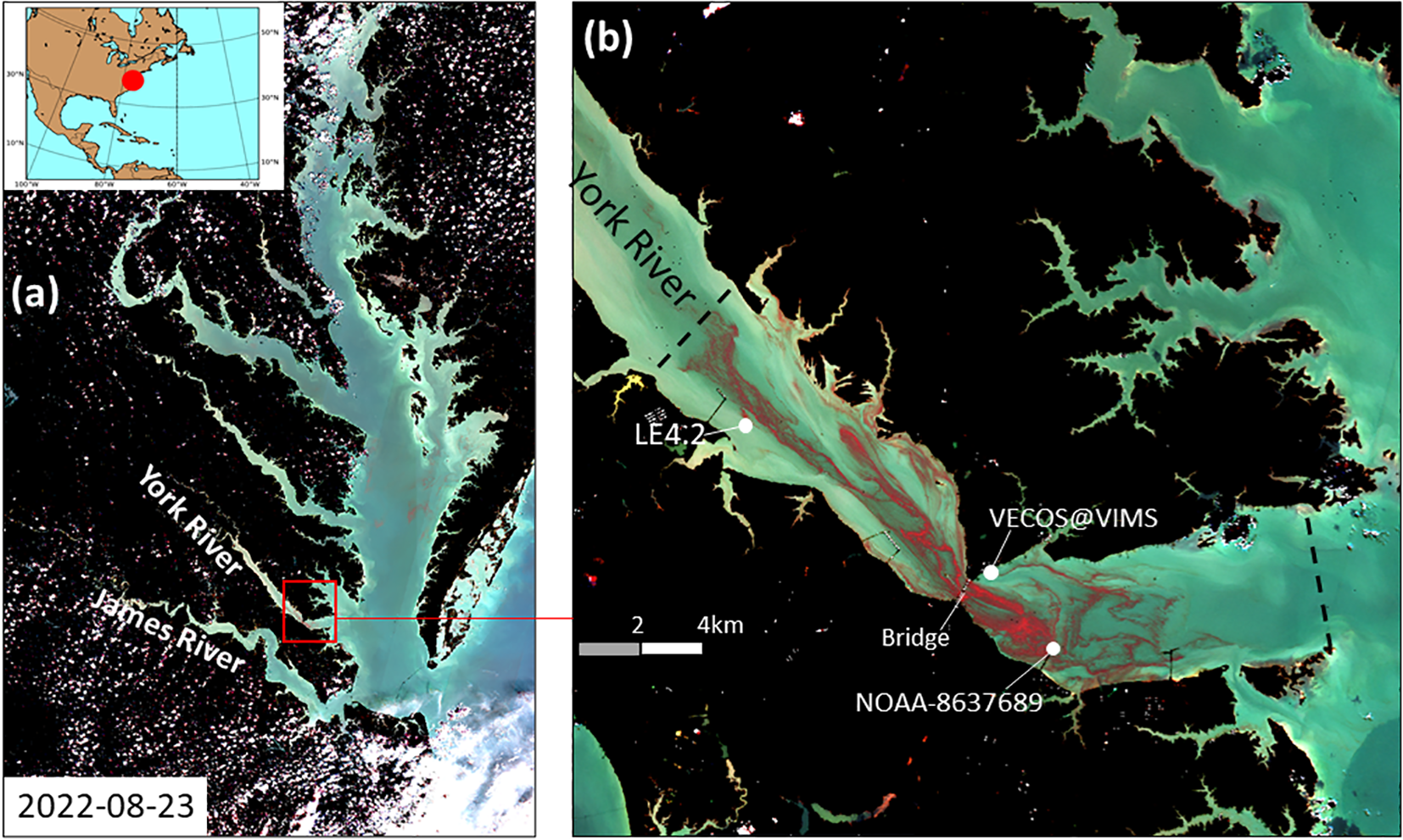
Figure 1. A regional map of Chesapeake Bay and the lower York River estuary. (a) A high-resolution false color composite generated from the Multispectral Instrument (MSI) onboard Sentinel-2 satellite image acquired on 23 August 2022. Red color indicates high M. polykrikoides biomass (Sentinel 2 image extracted from https://apps.sentinel-hub.com/eo-browser/). (b) A zoomed-in view of the false color composite satellite image in the lower York River on 23 August 2022. Also marked in (b) are region of lower York River (enclosed by two black dash lines) and monitoring stations (white dots): LE4.2 (maintained by Chesapeake Bay Program), NOAA-8637689, and VECOS station YRK004.50.

Methods

Satellite imagery for particle initiation

Near-daily satellite imagery was used to identify the location and intensity of blooms for model initiation during August-September of 2022. Satellite imagery at 300m resolution, was derived from the Ocean Land Colour Instrument (OLCI) aboard the Copernicus Sentinel-3 satellite obtained from the European Organization for the Exploitation of Meteorological Satellites (EUMETSAT) and processed by NOAA’s National Centers for Coastal Ocean Science (Wolny et al., 2020). The Sentinel-3 satellite reaches the Chesapeake Bay region around 15:00 (GMT) each day, i.e., 10:00 local time. The Red Band Difference (RBD), which is a proxy of relative Chlorophyll-a (Chl-a) fluorescence and commonly used to identify areas with high bloom biomass, was used to identify the locations of bloom pixels to initiate the model (Amin et al., 2009; Freitas and Dierrsen, 2019; Wolny et al., 2020; Jordan et al., 2021). From these pixels, a two-band coastal chlorophyll algorithm, using the red and near-infrared bands also referred as the red edge (RE10) was used to establish the concentration of the bloom and determine the number of particles (proportional to the Chl-a concentration) that were initiated at each corresponding pixel location (Gilerson et al., 2010; Wynne et al., 2021).

Images with extensive cloud cover were discarded. Of the available 61 images, 34 had at least 500 pixels (equivalent to 63% of satellite pixels in open water) with valid data in the lower York River (region marked in Figure 1). The 34 images were used to initialize the bloom in the particle tracking model over the entire bloom progression and to examine model performance over the period of 1-5 days after bloom initiation.

In situ water quality data

Monthly water quality data including salinity, water temperature, dissolved inorganic nitrogen (DIN), and total suspended solids (TSS) were obtained from Chesapeake Bay Program (CBP; http://data.chesapeakebay.net/WaterQuality). Salinity data were used to validate the hydrodynamic model, while the DIN and TSS data were interpolated bay-wide and used for the biological components of the particle tracking model. For each grid node in the hydrodynamic model, data at three nearest monitoring stations were used and interpolated based on the inverse distance weighted interpolation. In addition, continuous hourly monitoring data of salinity, temperature, and fluorescence-based Chl-a (Figure 2b) in the lower York River was obtained from the Virginia Estuarine and Coastal Observing System (VECOS; http://vecos.vims.edu) and used to compare with satellite-based Chl-a data and the hydrodynamic model during the 2022 bloom season.

Figure 2

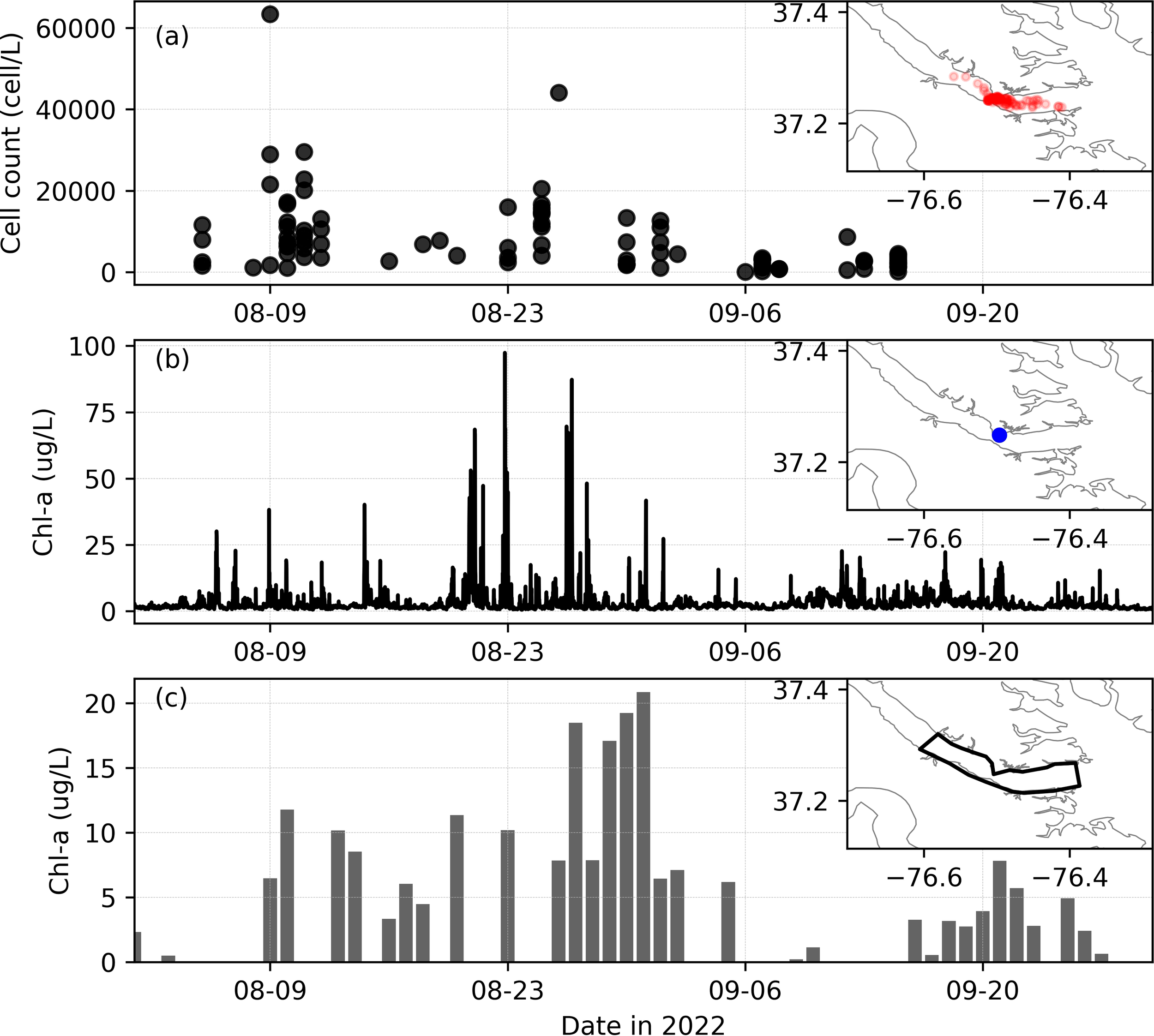
Figure 2. (a) Measured M. polykrikoides concentrations in the lower York River, with sampling locations shown in red circles in the map subset. (b) Measured Chl-a from a fluorometric sensor at VECOS station YRK005.40 (location marked in the subset). (c) Time series of Chl-a concentration averaged over a region of interest (marked with thick black polygon in the subset) from satellite imagery (OLCI, RE10). X and Y axes in the subsets represent longitude (deg) and latitude (deg), respectively.

In situ cell concentrations for satellite image verification (M. polykrikoides) were obtained from the Marine and Aquaculture Genetics lab at the Virginia Institute of Marine Science (VIMS) annually during the bloom season (August-October) from 2007-2022. Cell concentrations were estimated using both microscopic identification and quantitative PCR as previously described (Vandersea et al., 2017; Wolny et al., 2020). The water samples were collected at locations where the bloom was observed (Figure 2a). For the York River, these bloom samples were collected mostly in the lower York River region, similar to the area shown in Figure 1b.

Hydrodynamic model

We used a hydrodynamic model based on SCHISM (Semi-implicit Cross-scale Hydroscience Integrated System Model) to drive the particle tracking model. SCHISM (Zhang et al., 2016) is an open-source community-supported modeling system, based on mixed triangular-quadrangular unstructured horizontal grids and a flexible vertical coordinate system (Localized Sigma coordinates with Shaved Cell, or LSC2; Zhang et al., 2015), which was designed for the effective simulation of 3D baroclinic circulation across creek-to-ocean scales.

The hydrodynamic model was initially configured and validated for the mainstem of Chesapeake Bay (see the model domain in Figure 3a) and yielded good performance in reproducing the water level, temperature, and salinity in the bay’s mainstem (Ye et al., 2018). To simulate the hydrodynamics in the York River estuary, we refined the model grid to better represent the bathymetric features of the river (see refined mesh in Figure 3b). The deep channel (up to 15m deep) was better resolved by aligning the grid nodes along the 10m isobath. With the upgraded grid, model performance regarding salinity intrusion into the York River was greatly improved especially in the upper portion of the river (see Results Section).

Figure 3

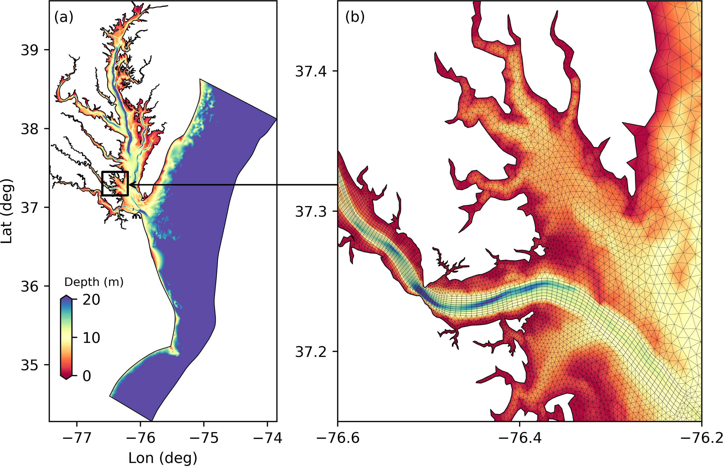
Figure 3. (a) Hydrodynamic model domain and bathymetry. (b) Zoomed-in view of the bathymetry and grid for the study area, including the York River and adjacent Mobjack Bay.

For this study, a one-year model run (January 01, 2022 to December 31, 2022) was conducted and the hydrodynamic fields including salinity, temperature, surface elevation, eddy diffusivity, and velocities were saved at hourly timesteps. We chose 2022 because there were numerous high-quality satellite images during the late summer bloom season, which lasted for 2 months (August-September). The multiple available satellite images allow for a more comprehensive evaluation of the particle-tracking model performance. Even though the focus is on the summer hydrodynamic conditions, we set the model to start on 01 January 2022 to account for model spin-up. Model results during the spin-up period are typically erroneous and not reliable. The error is primarily introduced by the uncertainty of the initial condition for the 3D salinity and temperature fields. The spin-up period is related to the residence time of the Chesapeake Bay, which is about 180 days (Du and Shen, 2016).

Particle tracking model

A Lagrangian particle tracking and biological (LPT-Bio) model originally developed for M. polykrikoides by Xiong et al. (2023) for the James River was modified for the York River. We modified the model to adjust for phytoplankton (M. polykrikoides) subsurface aggregation (now as an option in the model setting). We also tested the behavior of the coupled model approach and its potential use in a HAB early warning and forecasting framework by using satellite imagery collected throughout the bloom season (n=34 days) to release particles near-daily and assess how the model performed.

In the LPT-Bio model, output from the hydrodynamic model is saved and passed to a particle tracking model, making the HAB simulation highly efficient. In the particle tracking model, particle movement is governed by horizontal (Equations 1, 2) and vertical advection (Equation 3), swimming behavior, and diffusion through a random walk following (Chiu et al., 2018):

$\begin{array}{ll}{X}^{n+1}=X^n+\left(U+\frac{\partial K_x}{\partial x}\right)\Delta t+R\sqrt{6K_x\Delta t}& (1)\end{array}$

$\begin{array}{ll}{Y}^{n+1}=Y^n+\left(V+\frac{\partial K_y}{\partial y}\right)\Delta t+R\sqrt{6K_y\Delta t}& (2)\end{array}$

$\begin{array}{ll}{Z}^{n+1}=Z^n+\left(W+\frac{\partial K_z}{\partial z}+W_{swim}\right)\Delta t+R\sqrt{6K_z\Delta t}& (3)\end{array}$

where U, V and W are particle velocities in Cartesian coordinates x, y, and z; n is the time step index; R is a real random number with a mean of zero and a uniform distribution between -1 and 1; and K_x, and K_y are the eddy diffusivity (from the hydrodynamic model outputs), used to parameterize the random walk in the horizontal directions. A constant of 3×10^-4 m² s^-1 was used for K_z to parameterize the vertical random walk; this value was used by default in the original SCHISM particle tracking model. W_swim was the daytime (06:00-19:00) ascent and nighttime (19:00-06:00) descent velocities for M. polykrikoides. The timing was chosen according to the sun-rise, -set during the summer in the Chesapeake Bay region. For simplicity, we used the same value for both ascent and descent velocities. Algal bloom dynamics (i.e., mixotrophic growth, respiration, temperature-modulated mortality, and density-related aggregation settling; Equation 4) were included in the model to simulate variations in cell density, which are dynamically driven by environmental parameters (i.e., temperature, salinity, irradiance, and nutrients) and calibrated with observed M. polykrikoides distributions in the York River. Briefly, the cell density (C) recorded by particle i is controlled by:

$\begin{array}{ll}\frac{d{C}_i^t}{dt}=(G-R-M_T)C_i^t-M_{agg}& (4)\end{array}$

where R, M_T and M_agg are the respiration induced loss term, temperature-modulated mortality (Hofmann et al., 2021), and density-related aggregation settling loss term (Lima and Doney, 2004), respectively. G is the mixotrophic growth rate (Equations 5-1, 5-2), controlled by the optimal phototrophic growth (G^P, Equation 6), maximum heterotrophic growth (G^Ho, Equation 7), as well as salinity and temperature limitation functions (Qin et al., 2021).

$\begin{array}{ll}G=min[G_o^H+G_o^P,G_{opt}^{H}f(T)f(S)] , Daytime & \text{(5-1)}\end{array}$

$\begin{array}{ll}G=G_o^H, Nighttime& \text{(5-2)}\end{array}$

$\begin{array}{ll}{G}_o^P=G_{opt}^{P}f(T)f(S)min[f(I),f(DIN)]& (6)\end{array}$

$\begin{array}{ll}{G}_o^H=G_{opt}^{H}f(T)f(S)f(O{M}_{12})& (7)\end{array}$

where f(T), f(S), f(I), f(DIN) and f(OM) are temperature-, salinity- irradiance-, DIN-, and organic matter-limited functions, respectively. A full set of the governing and limitations functions, as well as the value of related parameters, can be found in Supplementary Tables S1, S2.

Particle release, biomass calculation, and model validation

For each of the 34 satellite-images available during the study period, we conducted a particle tracking simulation, tracking the time-varying biomass and location of each particle for 15 days following release. Particles were only released in the York River and at locations where satellite pixels had an RBD value >2×10^-4 (dimensionless), indicating high bloom concentrations. Each particle carries 1×10⁷ cells initially, following the same strategy in Xiong et al. (2023). Therefore, the number of particles (npar) released at each satellite pixel was given as $npar=c\times {10}^{-7}$, where c is the M. polykrikoides cell count calculated from the RE10 estimated Chl-a concentration using a conversion factor of 1.69×10^-8 mg Chl-a cell^-1 (Hofmann et al., 2021). Depending on the Chl-a value as well as the cloud cover, the number of particles varied between 112 and 184,388, with a median value of ~90,000 over the 34 releases.

To compare the modeled particle distribution with satellite measurements, we back-calculated the biomass in a meshed grid (300m × 300m, same spatial resolution as the satellite image) using the same cell to Chl-a conversion from Hofmann et al. (2021). The calculated biomass sums the number of particles within a given grid and the biomass represented by each of the particles.

Due to the availability of near-daily satellite images, we were able to examine the performance of each particle tracking simulation 1-5 days into the future. For instance, for simulation with particles released on 09 August 2022, its performance on days 1, 4, and 5 could be assessed by comparing the model predictions and the satellite image on 10 August, 13 August, and 14 August, respectively (Figure 4). To quantitatively assess the model performance, we calculated two indices: true positive prediction (TPP) and true negative prediction (TNP). TPP was calculated as the ratio of the number of pixels with Chl-a > 10 ug L^-1 (~6·10⁵ cells L^-1) in both the satellite image and model to the total number of pixels with Chl-a > 10 ug L^-1 in satellite image. Similarly, TNP was calculated as the ratio of pixels with Chl-a< 10 ug L^-1 in both the satellite image and model to the total number of pixels with Chl-a<10 ug L^-1 in the satellite image. The criteria of 10 ug L^-1 was selected to highlight the intense bloom area and also because of the relatively high background Chl-a concentration (e.g., during the non-bloom period) based on the satellite images in this tributary. A large TPP value (e.g., >0.5) indicates good model performance in capturing the high Chl-a distribution. Because the majority of the lower York River in 2022 had no bloom condition, TNP is typically large (>0.9). For model performance assessment, we also calculated the RMSE (Equation 8).

Figure 4

Figure 4. Available satellite imagery (OLCI, RE10 algorithm) for Chl-a concentrations in the lower York River from August-September 2022. Land is white. No satellite data was available for the black regions (e.g., obscured by clouds).

$\begin{array}{ll}RMSE=\sqrt{\frac{{{\displaystyle \sum }}_i^N{(x_i-y_i)}^2}{N}}& (8)\end{array}$

where x_i is the modeled result at a given sampling location (i.e., the pixel location in satellite image) and y_i is the observed value from remote sensing data.

Results

Satellite observations of the 2022 M. polykrikoides bloom

In 2022, the M. polykrikoides bloom lasted for ~ 2 months (August-September, 2022), while in previous years, the bloom typically lasted for about one month (mostly in August). The evolution of the two-month M. polykrikoides bloom was well captured by satellite imagery (Figure 4). Elevated surface Chl-a concentrations first appeared in the York River on 03 August. The bloom’s intensity increased for about two weeks until August 16 when the surface bloom was no longer visible by satellite. The reduced surface bloom concentration was likely due to windy induced mixing which drove the bloom subsurface making it unobservable by satellite. After 17 August, the bloom continued for another two weeks, with extremely high surface Chl-a concentrations (>50 ug L^-1) throughout the lower York River. The surface bloom moved back and forth within the lower York River during this period under the influence of tidal and wind-driven currents. Because of the dominant semi-diurnal tide (M2, tidal period of 12.42 hr), the tidal phase differs between days when the satellite image was captured.

The bloom disappeared around 10 September when the satellite imagery no longer observed a surface bloom (Figure 4). Between 11 and 15 September, there were no high-quality satellite images. The bloom reappeared after 16 September. The underlying reason for the bloom’s temporal disappearance is yet to be understood, but it was likely related to temperature and salinity variations. Specifically, around 10 September, salinity was steady (~22) while temperature dropped slightly but was still above 25°C (Figures 5a, b). However, vertical mixing induced by strong winds likely decreased surface concentrations of algal biomass, similar to what happended in mid-August (Figure 5c). There was also a precipitation event on 11 September, followed by a slight increase in freshwater inflow (Figure 5d). The increased freshwater input may have also flushed out many of the phytoplankton cells (e.g., M. polykrikoides) in the lower York River, leading to lower Chl-a concentrations.

Figure 5

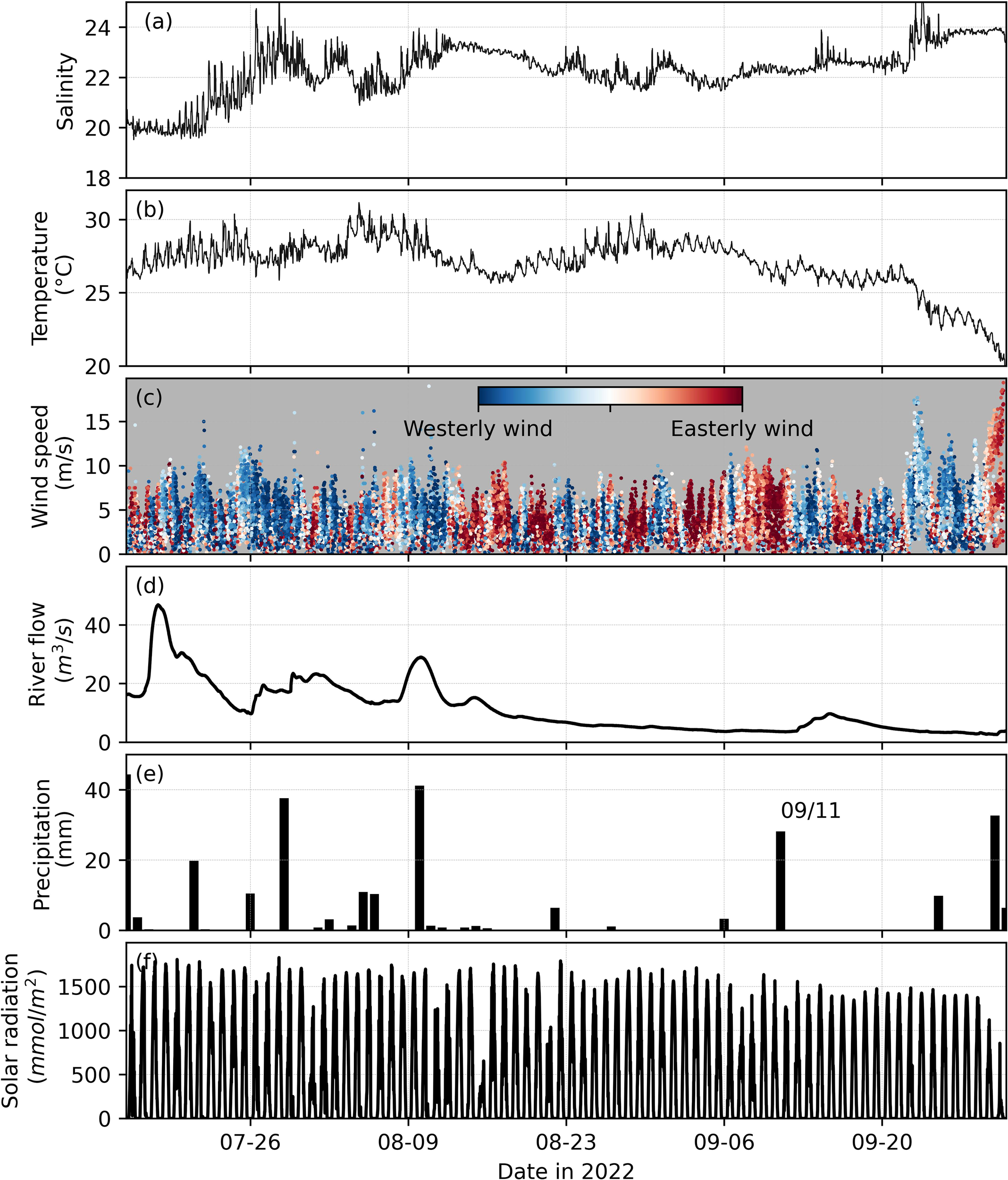
Figure 5. Physical conditions in the summer of 2022, including: (a) salinity and (b) temperature at VECOS station YRK005.40. (c) Wind speed measured at NOAA gauging station 8637689, with red dots indicating easterly wind, blue dots indicating westerly wind, and white dots indicating wind from the north or south. (d) River flow from the Mattaponi and Pamunkey Rivers. (e) Daily precipitation and (f) total photosynthetically active radiation (PAR) measured at station CBVTCMET maintained by the Chesapeake Bay-Virginia National Estuarine Research Reserve (data from https://cdmo.baruch.sc.edu/dges/).

When averaged over the lower York River, the mean Chl-a concentration based on the satellite imagery shows consistent results with the hourly fluorescence-based Chl-a measured at a VECOS monitoring station (Figures 2b, c). The VECOS station is located on the northern side of the river and, due to the patchiness of bloom population, did not reflect the intensity of the entire lower York River bloom. Due to the narrowing of the river channel near the VECOS station (see Figure 1b), the highest concentrations of the bloom tended to aggregate on the southern side of the river (Figure 4) during the bloom period. When the bloom was most intense in the middle or southern side of the York River, the high biomass was likely diffused or advected to the north, leading to a higher concentration of Chl-a at the VECOS station. In summary, both datasets confirmed the peak bloom period in late August and the bloom reappearance in mid-September after ~ 10 days with low Chl-a in early September.

Over the two-month period, environmental conditions were also examined in the York River to reveal possible physical mechanisms that led to the long-lasting bloom. Overall, the physical conditions during August and September (low river flow, high temperature, and prevalent easterly winds; Figure 5), likely favored HAB growth in the lower York River. Salinity and water temperature were relatively stable, with salinity ranging between 21-23 and temperature maintaining relatively high values above 25 °C for most of the time period (Figures 5a, b), conditions that were especially favorable for M. polykrikoides. The temperature dropped dramatically to less than 25°C after September 20^th. The temperature drop, along with strong westerly winds that favor seaward movement of algae in lower York (Figures 5b, c), likely explains the end of the bloom in late September. In addition, during the bloom period, the river flow rate was<5 m³/s on average (~10% of the mean river flow in 2022; Figure 5d). The low river flow led to a steady but gradual increase in salinity during the study period. The low freshwater input would also lead to longer retention time for blooms in the lower York and less flushing of the algae out of the estuary into the Chesapeake Bay proper. The retention of algae could be also enhanced by the prevalent easterly wind (blowing from the east toward the upstream). The upstream wind tends to weaken the estuarine circulation (Chen and Sanford, 2009), leading to smaller down-estuary surface current.

Hydrodynamic model performance

The hydrodynamic model accurately reproduced the observed salinity, temperature, and water level in the lower York River for summer 2022 (Figure 6). The good match between the hydrodynamic model results and water level and salinity observations suggests the model is reliable in representing York River hydrodynamic transport and mixing processes. There are, however, notable discrepancies in modeled temperature in the first four months (i.e., during the model spin-up period). The error is introduced by inaccurate initialization of the temperature and salinity fields from the monthly field data. The magnitude of the error diminishes over time during model spin-up. We also note discrepancies in measured and modeled salinity in late September. These discrepancies could be induced by a variety of factors including uncertainty in freshwater input, atmospheric forcings (e.g., wind), and errors originating from the hydrodynamic model in the main stem of Chesapeake Bay. The root mean square errors (RMSEs) between model and observation are 0.76 (salinity), 1.52°C (temperature), and 6.83cm (water level) over the entire year. For estuarine modeling, RMSE below 2 (salinity), 2°C (temperature), and 10 cm (water level) typically indicates the model is reliable. For instance, the SCHISM model for the mainstem of Chesapeake Bay (Ye et al., 2018) has RMSE of 1.5 for surface salinity, 1.6°C for surface temperature, and 11 cm for water level. For the summer of 2022, the study period of interest, the RMSE is even smaller and therefore the hydrodynamic model was deemed reliable for this study (Figure 6).

Figure 6

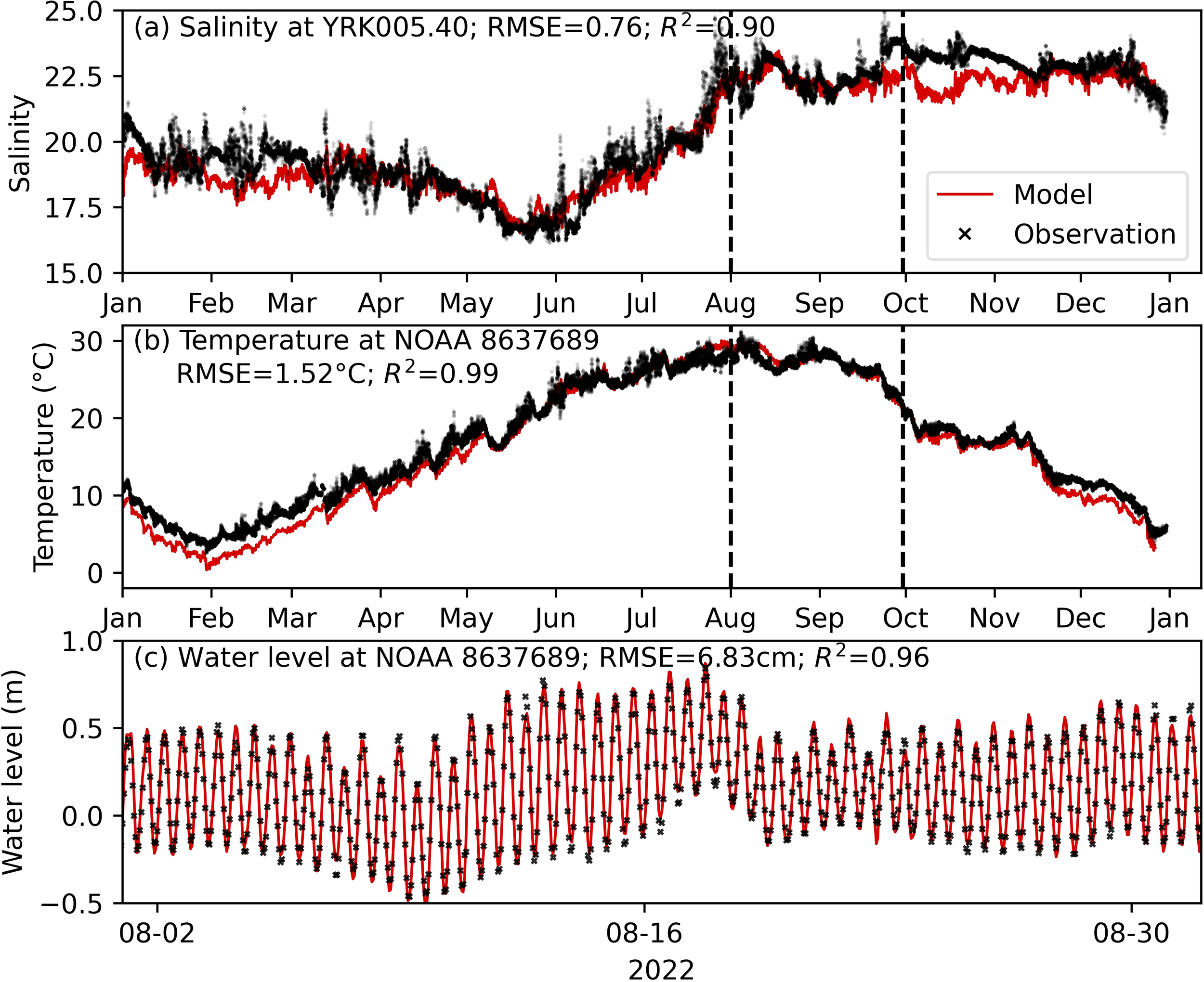
Figure 6. Modeled and observed salinity, temperature, and water level in the lower York River. Note the different e x-axis limits in (c) compared to (a, b). Vertical lines in (a, b) mark the period of August-September, the bloom period in 2022. RMSE (root mean square error) and R² (coefficient of determination) for the entire-year comparison between model and observation are shown at the top of each panel.

The performance of the hydrodynamic model is good primarily due to the reliability of the model in the Chesapeake Bay mainstem (Supplementary Figure S1) as well as the refinement of the model grid for the York River. Compared to Ye et al. (2018), the saltwater intrusion in the York River was better resolved (supplemental Supplementary Figure S2). Grid refinement in the York River, especially for the deeper part of the river channel, enhances the saltwater intrusion.

Particle-tracking model performance

With multiple high-quality satellite images, we were able to assess the performance of the particle tracking model. Taking the particle release on 27 August 2022 (near the bloom peak) as an example, the model appropriately captures the spatial distributions of the M. polykrikoides bloom. One particularly notable comparison was on 31 August 2022 (4 days after particle release), when the model nearly perfectly captures the bloom distribution, with a high concentration of Chl-a in the middle deep channel downstream of the York River bridge and on the northern side of the estuary upstream of the bridge. The match between the model and observed satellite imagery is also notable from the high TPP and TNP values. On 31 August 2022, TPP was 0.84 while TNP was 0.90. The model also accurately captured the overall spatial pattern even 9 days (i.e., on 05 September 2022) after particle release (Figure 7). For instance, both the model and satellite image showed the bloom concentrated along the south side of the York River, while the bloom location appears to move with the incoming and outgoing tide. TPP values are consistently high throughout the 10 days following particle release, with a value >0.72, indicating the majority of the bloom locations with Chl-a >10 ug L^-1 were captured by the model.

Figure 7

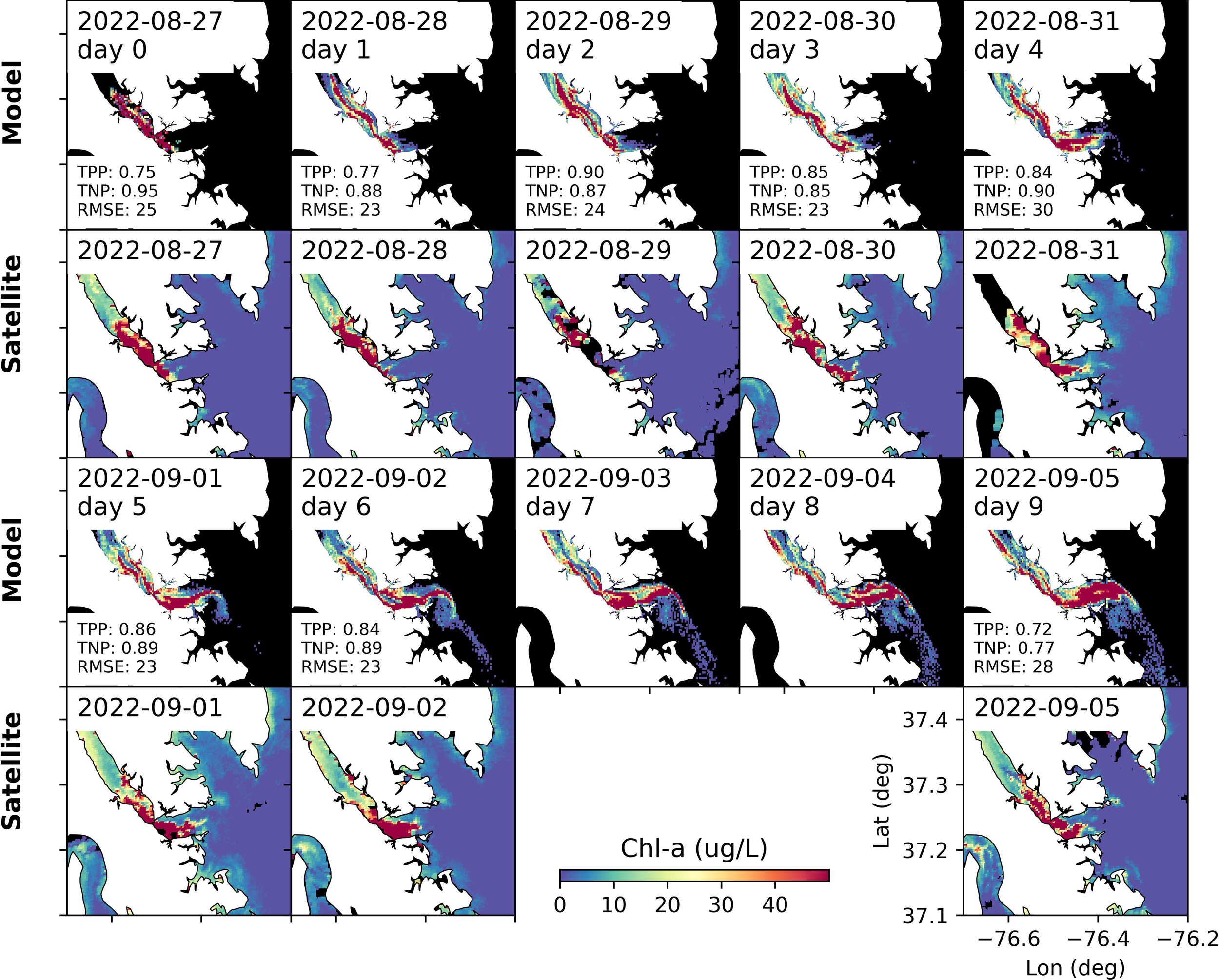
Figure 7. Comparison between modeled and satellite-observed Chl-a in lower York River. The model results are from experiments with particles released on 27 August 2022. The first and third rows are from the model, while the second and fourth rows are satellite data. TPP, TNP, and RMSE values are shown in the text. There were no high-quality satellite images for 03 September 2022 or 04 September 2022.

The high model performance is consistent for almost all release experiments. Due to cloud cover, not every release experiment has corresponding satellite imagery to compare and validate the model for a specific number of days after particle release. Taking a 3-day prediction as an example, there were 20 model runs which had corresponding satellite imagery that could be used for model-observation comparisons (Figure 8). Overall, the model generally captured HAB spatial distribution well, with median TPP and TNP values of 0.50 and 0.96 for the 3-day prediction, respectively, and a median RMSE of 23 ug L^-1. Note that the large RMSE is partially due to the large magnitude of chlorophyll concentration during the bloom period. Comparisons for days 1, 2, 4, and 5 can be found in the supplemental materials (Supplementary Figures S3-S6).

Figure 8

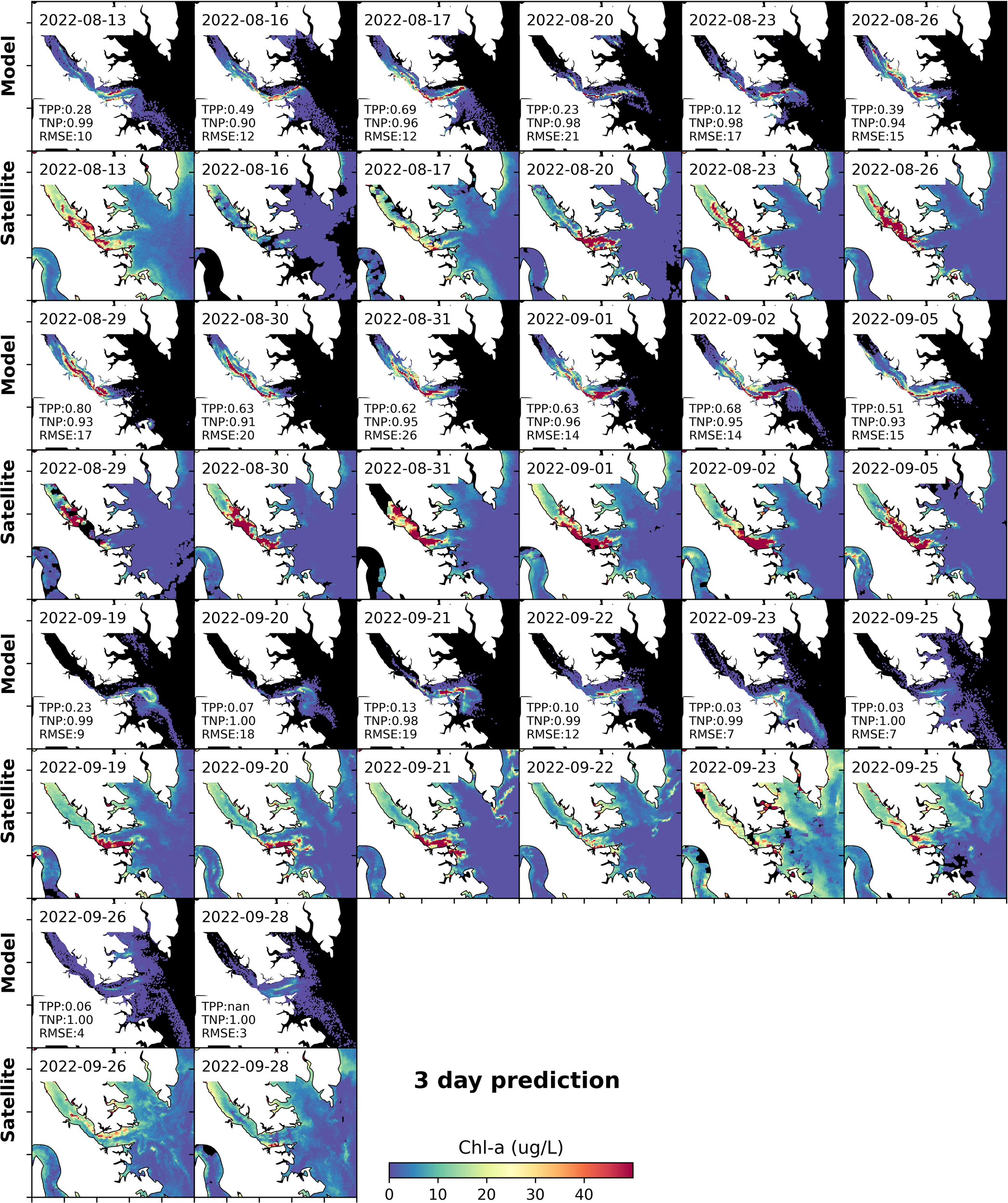
Figure 8. Modeled and observed Chl-a 3 days after model initialization from 34 particle tracking model runs. The first, third, fifth, and seventh rows are day-3 results from multiple model runs; corresponding satellite images are shown in the second, fourth, sixth and eighth rows. TPP, TNP, and RMSE are displayed in the model run panels.

However, the model skill typically diminishes for longer prediction time periods (>5 days). The decreasing model performance could be due to multiple factors including error in the modeled hydrodynamic field, limited field nutrient data for model calibration, uncertainty in biogeochemical processes, and inherent uncertainty in the Lagrangian model (e.g., diffusion). We also found that the bloom distribution pattern was altered when considering different swimming behaviors. In addition, sensitivity tests conducted during this study (Figure 9; more details in the Discussion Section), demonstrated that including subsurface aggregation improved model performance.

Figure 9

Figure 9. (a) Satellite image on 21 September 2022 and (b-d) results from the model sensitivity tests (3 days after particles released on 18 September 2022). Sensitivity tests included subsurface aggregation (no subsurface aggregation or 2m subsurface aggregation) and a maximum depth set to 15 m or 5 m.

Discussion

Overall, results show a good match between model predictions and available satellite observations suggesting the success of the coupled satellite imagery-particle tracking model framework. To further advance model results, we also conducted a series of sensitivity tests to better parameterize algal biological behaviors, especially vertical swimming. In the following sections, we will discuss the sensitivity of model performance to different parameterizations of M. polykrikoides swimming behavior including maximum swimming depth and subsurface aggregation depth. Finally, we discuss how this coupled model framework could be applied to provide short-term (1-3 day) forecasts of M. polykrikoides bloom intensity and location within the lower York River Estuary and the wider lower-Chesapeake Bay to provide advanced warning of potential HAB impacts to coastal resource managers, shellfish operators, and the general public.

Model sensitivity to M. polykrikoides swimming parameterization

While the diel vertical migration is well known as one key behavior of M. polykrikoides (Park et al., 2001), there is still uncertainty about their potential swimming speed. Field measurements and lab experiments suggest a range of 10-70 m d-1, depending on chain length, life-cycle stage (Sohn et al., 2011) and external environmental conditions such as water temperature, salinity and light conditions (Lim et al., 2022). Field measurement in Lafayette River, a sub-tributary of the Chesapeake Bay, estimated a mean swimming speed of 31 m d^-1, with a maximum of 60 m d^-1 (Clayton et al., 2024). Using a holography system, Sohn et al. (2011) measured the swimming speed of M. polykrikoides and found a mean swimming speed of 33 m d-1 for solitary cells and 73 m d^-1 for 8-cell chains. Additionally, in their modeling study, Xiong et al. (2023) demonstrated how different swimming speeds affected the spatial distribution of M. polykrikoides in the James River.

In addition to swimming speed, estuarine hydrodynamics also influence the vertical distribution of phytoplankton in the water column and throughout the estuary. For example, due to estuarine circulation and stratification, phytoplankton cells at the surface can be advected out of the estuary while cells in the bottom waters are transported into the estuary at depth. To take advantage of this estuarine circulation and to maximize light and nutrient uptake, it is generally assumed that phytoplankton, including M. polykrikoides, aggregate near the surface during the day and swim down to the deeper waters at night (Erga et al., 2015). Depending on the water column depth, pycnocline depth, and phytoplankton swimming speed, phytoplankton may take hours to swim to the surface from different depths. For instance, with a swimming speed of 20 m d^-1 and a maximum depth of 15 m, it would take ~18 hours for phytoplankton in the bottom waters to reach the surface. If swimming starts near dawn, the phytoplankton will reach the surface at dusk, thus missing the favorable solar radiation conditions during the day, which is unfavorable for phytoplankton growth. However, for shallower regions (e.g., 5 m depth), a swimming speed of 20 m d^-1 could be adequate for phytoplankton to swim from the bottom waters to the surface in a reasonable amount of time. To assess the impact of swimming speed on the distribution of M. polykrikoides cells, we tested different swimming speeds (10-40 m d^-1), within the range of reported lab and field studies, which had limited effect on the model results. This may be due to the shallow depth of most of the estuary (<5 m) (Figure 3b).

In addition to swimming speed, we also wanted to test a maximum swimming depth to further parameterize M. polykrikoides vertical migration. Therefore, we examined how setting a maximum depth (e.g., 5 m and 15 m) affects M. polykrikoides vertical and horizontal distribution. The difference in model results is notable when using different maximum depths (Figure 9). With a smaller maximum depth, M. polykrikoides cells tend to aggregate at the surface and be subject to stronger flushing forces, leading to a higher concentration downstream. Following this sensitivity test, we used a maximum swimming depth of 5 m to further constrain M. polykrikoides vertical migration.

In addition, subsurface aggregation of M. polykrikoides could also affect the vertical and horizontal distribution of cells. Phytoplankton may not always settle to the bottom but aggregate at a certain depth. Subsurface aggregation is also common in the open ocean, where maximum phytoplankton concentrations are often found at subsurface depths near the nutricline (Cullen, 2015; Baldry et al., 2020; Masuda et al., 2021). The subsurface aggregation is typically weak in nearshore environments where turbidity is often higher (Lu et al., 2010). Depending on light conditions, the subsurface aggregation (or subsurface chlorophyll maximum) could also occur in coastal waters with low turbidity (Lim et al., 2022). For instance, Lim et al. (2022) found the highest density of M. polykriokoides at a depth of 3-6 m during the day off the southern coast of Korea, concluding that M. polykrikoides may have used subsurface aggregation to avoid a heat wave which coincided with the field survey (water temperatures exceeding 29°C). Measurements by VECOS in the lower York River also suggest subsurface aggregation of phytoplankton at depths of 1-3 m in early August of 2011 and 2012 (see Supplementary Figures S7, S8). In coastal waters, subsurface phytoplankton aggregation could be used as a strategy to avoid high solar radiation and elevated water surface temperatures during the summer, however, the underlying mechanisms are yet to be investigated. Considering the potential subsurface aggregation, we also carried out model sensitivity tests regarding the impact of a subsurface aggregation depth on M. polykrikoides distribution. We choose 2 m as the subsurface aggregation depth considering the observed aggregation in York River (Supplementary Figures S7, S8). In this case, the biomass of the top 2 m was calculated to compare with the satellite image, in contrast to previous model tests where the top 1 m biomass was calculated.

Our model sensitivity tests suggested that a subsurface aggregation of 2 m and maximum depth of 5 m best captured the spatial distribution of the M. polykrikoides bloom (Figures 9, 10). For example, when releasing particles on 17 September 2022, the model with both the maximum swimming depth constraint and subsurface aggregation gave the best match between the model and satellite images on 22 September 2022, 3 days after particle release. The maximum swimming depth led to higher phytoplankton biomass on the southern side of the river, while the base case (i.e., maximum depth = 15 m) showed much higher concentrations along the northern side of the river. With the subsurface aggregation depth constraint, the modeled M. polykrikoides distribution was more aligned with the satellite image (Figure 9). We carried out sensitivity tests for all the satellite available days and the results of 170 model runs (5 settings for 34 release days) are shown in Figure 10. The best model performance in terms of TPP was from the model runs with both subsurface aggregation (2 m) and a maximum depth of 5 m, with median TPP increased to 0.70 from 0.50 in the base case (without subsurface aggregation and with a maximum depth of 15m). Interestingly, the two best settings are with a maximum depth of 5 m with and without subsurface aggregation. For those with a maximum depth of 15 m (i.e., no maximum depth limitation since the estuary is<15 m), the model performance increases when increasing the subsurface aggregation from 0 m to 2 m. These model sensitivity tests suggest M. polykrikoides likely uses a subsurface aggregation depth, similar to what was observed by Lim et al. (2022). Additional field studies are needed to confirm this hypothesis.

Figure 10

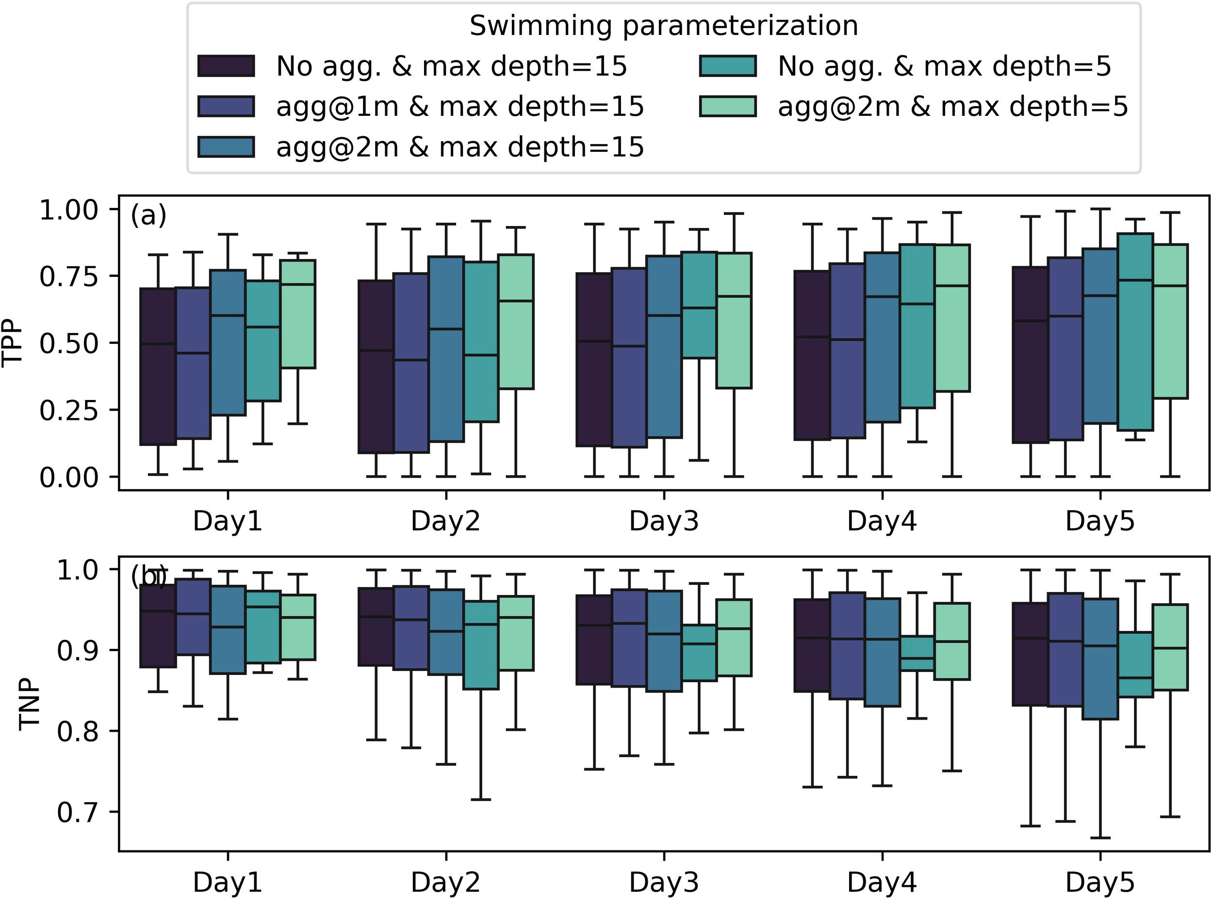
Figure 10. TPP and TNP values for different parameterization of M. polykrikoides swimming behavior. The error bar indicates one standard deviation. In the base run (black color), there was no subsurface aggregation and the maximum depth was set to 15 m, which is often deeper than the depth of the York River Estuary.

Model limitations

Overall, the model reasonably produced the variability during the summer 2022 M. polykrikoides bloom in the York River Estuary. However, uncertainties between the observations (satellite imagery) and model exist. For example, a) the model tends to have a longer high-Chl-a feature stretching into the upper York River, which was not observed in the satellite imagery; b) high values of Chl-a are also more concentrated along the middle deep channel in the model; and c) the model tends to overestimate the Chl-a concentrations at the mouth of the York River, especially 5+ days after particle release. The bias is also notable from the TNP. When TNP is<0.8 (e.g., on 05 September 2022 in Figure 8), the model is generally thought to over-predict the bloom region. Below, we discuss key limitations of this modeling approach.

First, there is limited availability of nutrient data (i.e., 6 locations measured monthly in York River). Therefore, there are substantial uncertainties in the nutrient field used in the model prior to and during the bloom. Linear interpolation (as used in this study) with the monthly data tends to neglect realistic variations. Second, nutrient consumption and speciation were not considered in the particle tracking model. Further studies looking at the role of nutrient speciation on the growth and limitation of M. polykrikoides could help to further refine the model. In addition, lacking the dynamic balance between nutrient availability and phytoplankton uptake tends to overestimate the growth rate, especially during the bloom peak. Ideally, the biomass should be included as a parameter when determining the nutrient limitation function. Finally, we did not include species competition or succession. As the in situ phytoplankton data shows, there can be a succession of M. polykrikoides to Alexandrium monilatum (A. monilatum) in the late summer to fall (Supplementary Figure S9). However, the mechanisms responsible for the shift from M. polykrikoides to A. monilatum are not well understood and were not included in this modeling effort.

In addition to nutrient dynamics, small-scale hydrodynamics may be not well resolved with the setting of the current hydrodynamic model, as the model is currently using the atmospheric product, North American Regional Reanalysis (NARR), which has a resolution of ~28 km. The transport and mixing processes within a small, river-dominated estuary, like the York River, are especially sensitive to the wind field. Considering the width of York River (2-5 km), using the NARR to drive the model will inevitably over-smooth the hydrodynamic field and miss small-scale variability in water currents within the estuary.

Finally, using satellite Chl-a imagery for bloom initiation and validation may also introduce errors. For instance, overestimates in bloom concentration may occur when other Chl-a containing phytoplankton co-occur. Simultaneously, underestimates may occur during wind mixing events, as the bloom is mixed to the subsurface (Li et al, 2020). Additional samples of M. polykrikoides distribution and other co-occurring phytoplankton species throughout the water column are necessary. In addition, a direct correlation between satellite chlorophyll to cell concentrations for the RE10 algorithm is still being investigated. Wynne et al. (2022) demonstrated that the absolute error in field Chl-a to satellite Chl-a was 36%. While absolute concentrations of M. polykrikoides from satellites have inherent error, relative changes in bloom concentrations identified by satellite remote sensing are reliable in providing useful information to managers in the region.

Conclusion

In this study, we demonstrate the use of a coupled satellite imagery-numerical modeling approach, as an effective way to simulate and eventually forecast the distribution of HABs in the York River. The model framework presented here shows great potential in predicting bloom movement and location over 1-5 days in the future. In addition, we highlight the important role of M. polykrikoides swimming behavior to appropriately model the biomass distribution vertically and horizontally, particularly the subsurface aggregation, which has not been considered in previous modeling efforts.

Ultimately, this study serves as an example of a ‘data-assimilative’ HAB forecasting effort, which can be used to provide useful guidance for: 1) supporting local tourism and recreation including recreational fishing; 2) guiding state sampling of bloom location on a daily basis; and 3) providing short-term forecasts to the aquaculture community to aid management decisions such as the movement of shellfish, and treatment of incoming water for shellfish hatcheries.

With the successful test in the York River, the modeling framework can be applied to other coastal systems. Efforts are currently underway to expand the modeling domain for the entire lower Chesapeake Bay where M. polykrikoides blooms occur and move towards an operational forecast system in the region. For instance, in 2023 a bloom was initiated off Tangier Sound on the eastern shore bordering Maryland and Virginia following identification in near-real time satellite imagery. The bloom was confirmed by the Virginia Department of Health and the MD Department of the Environment to be M. polykrikoides. Preliminary results (not shown) indicate that the model successfully predicted the transport of the bloom across the Bay to the mouth of the Rappahannock River, while underestimating bloom concentration at the surface. Therefore, adjustments in the ecological parameterizations will be necessary to accurately account for bloom concentration at the surface. With the proper parameterization, next steps will also focus on applying a similar modeling approach to other HAB species in lower Chesapeake Bay, such as Alexandrium monilatum.

Data availability statement

The original contributions presented in the study are included in the article/Supplementary Material. Further inquiries can be directed to the corresponding author.

Author contributions

XY: Conceptualization, Data curation, Formal analysis, Investigation, Methodology, Software, Visualization, Writing – original draft, Writing – review & editing. MT: Conceptualization, Formal analysis, Funding acquisition, Investigation, Project administration, Resources, Supervision, Writing – original draft, Writing – review & editing. JS: Conceptualization, Investigation, Methodology, Supervision, Writing – review & editing. YL: Conceptualization, Formal analysis, Investigation, Methodology, Writing – review & editing. AH: Conceptualization, Formal analysis, Investigation, Methodology, Writing – review & editing. GS: Data curation, Writing – review & editing. KR: Data curation, Investigation, Writing – review & editing.

Funding

The author(s) declare that financial Support was received for the research and/or publication of this article. This research was funded by the National Centers for Coastal Ocean Science (NCCOS) of the National Oceanic and Atmospheric Administration (NOAA). This research was supported in part by an appointment to the NOAA Research Participation Program administered by the Oak Ridge Institute for Science and Education (ORISE) through an interagency agreement between the U.S. Department of Energy (DOE) and NOAA. ORISE is managed by ORAU under DOE contract number DE-SC0014664. Research was supported in part by funding from the Virginia Department of Health.

Acknowledgments

We sincerely thank Jilian Xiong, Jiabi Du, Kyeong Park, and Joseph Zhang’s group for their help in the original model development. We also thank the editor and two reviewers for providing helpful comments to revise this manuscript.

Conflict of interest

Author XY, YL were employed by the company CSS, Inc.

The remaining authors declare that the research was conducted in the absence of any commercial or financial relationships that could be constructed as a potential conflict of interest.

Generative AI statement

The author(s) declare that no Generative AI was used in the creation of this manuscript.

Publisher’s note

All claims expressed in this article are solely those of the authors and do not necessarily represent those of their affiliated organizations, or those of the publisher, the editors and the reviewers. Any product that may be evaluated in this article, or claim that may be made by its manufacturer, is not guaranteed or endorsed by the publisher.

Author disclaimer

The scientific results and conclusions, as well as any views or opinions expressed herein, are those of the author(s) and do not necessarily reflect those of NOAA, the Department of Commerce (DOC), Department of Energy (DOE), or ORAU/ORISE.

Supplementary material

The Supplementary Material for this article can be found online at: https://www.frontiersin.org/articles/10.3389/fmars.2025.1561340/full#supplementary-material

References

Amin R., Zhou J., Gilerson A., Gross B., Moshary F., Ahmed S. (2009). Novel optical techniques for detecting and classifying toxic dinoflagellate Karenia brevis blooms using satellite imagery. Optics Express 17, 9126–9144. doi: 10.1364/OE.17.009126

PubMed Abstract | Crossref Full Text | Google Scholar

Anderson D. M., Fensin E., Gobler C. J., Hoeglund A. E., Hubbard K. A., Kulis D. M., et al. (2021). Marine harmful algal blooms (HABs) in the United States: History, current status and future trends. Harmful Algae 102, 101975. doi: 10.1016/j.hal.2021.101975

PubMed Abstract | Crossref Full Text | Google Scholar

Baldry K., Strutton P. G., Hill N. A., Boyd P. W. (2020). Subsurface chlorophyll-a maxima in the southern ocean. Front. Mar. Sci. 7, 671. doi: 10.3389/fmars.2020.00671

Crossref Full Text | Google Scholar

Chen S.-N., Sanford L. P. (2009). Axial wind effects on stratification and longitudinal salt transport in an idealized, partially mixed estuary. J. Phys. Oceanography 39, 1905–1920. doi: 10.1175/2009JPO4016.1

Crossref Full Text | Google Scholar

Chiu C.-M., Huang C.-J., Wu L.-C., Zhang Y. J., Chuang L. Z.-H., Fan Y., et al. (2018). Forecasting of oil-spill trajectories by using SCHISM and X-band radar. Mar. pollut. Bull. 137, 566–581. doi: 10.1016/j.marpolbul.2018.10.060

PubMed Abstract | Crossref Full Text | Google Scholar

Clayton S., Chrabot J. B., Echevarria M., Gibala-Smith L., Mtogatas K., Bernhartdt P., et al. (2024). Diel vertical migration rates of the dinoflagellate species Margalefidinium polykrikoides in a lower Chesapeake Bay tributary. Frontier Microbiol. 15. doi: 10.3389/fmicb.2024.1378552

PubMed Abstract | Crossref Full Text | Google Scholar

Cullen J. J. (2015). Subsurface chlorophyll maximum layers: enduring enigma or mystery solved? Annu. Rev. Mar. Sci. 7, 207–239. doi: 10.1146/annurev-marine-010213-135111

PubMed Abstract | Crossref Full Text | Google Scholar

Du J., Shen J. (2016). Water residence time in Chesapeake Bay for 1980–2012. J. Mar. Syst. 164, 101–111. doi: 10.1016/j.jmarsys.2016.08.011

Crossref Full Text | Google Scholar

Erdner D. L., Dyble J., Parsons M. L., Stevens R. C., Hubbard K. A., Wrabel M. L., et al. (2008). Centers for Oceans and Human Health: a unified approach to the challenge of harmful algal blooms. Environ. Health 7, S2. doi: 10.1186/1476-069X-7-S2-S2

PubMed Abstract | Crossref Full Text | Google Scholar

Erga S., Olseng C., Aarø L. (2015). Growth and diel vertical migration patterns of the toxic dinoflagellate Protoceratium reticulatum in a water column with salinity stratification: the role of bioconvection and light. Mar. Ecol. Prog. Ser. 539, 47–64. doi: 10.3354/meps11488

Crossref Full Text | Google Scholar

Fortin S. G., Song B., Anderson I. C., Reece K. S. (2022). Blooms of the harmful algae Margalefidinium polykrikoides and Alexandrium monilatum alter the York River Estuary microbiome. Harmful Algae 114, 102216. doi: 10.1016/j.hal.2022.102216

PubMed Abstract | Crossref Full Text | Google Scholar

Freitas F. H., Dierrsen H. M. (2019). Evaluating the seasonal and decadal performance of red band difference algorithms for chlorophyll in an optically complex estuary with winter and summer blooms. Remote Sens. Environ. 231, 111228. doi: 10.1016/j.rse.2019.111228

Crossref Full Text | Google Scholar

Gilerson A. A., Gitelson A. A., Zhou J., Gurlin D., Moses W., Ioannou I., et al. (2010). Algorithms for remote estimation of chlorophyll-a in coastal and inland waters using red and near infrared bands. Optics Express 18, 24109–24125. doi: 10.1364/OE.18.024109

PubMed Abstract | Crossref Full Text | Google Scholar

Gobler C. J. (2020). Climate change and harmful algal blooms: insights and perspective. Harmful Algae 91, 101731. doi: 10.1016/j.hal.2019.101731

PubMed Abstract | Crossref Full Text | Google Scholar

Gobler C. J., Burson A., Koch F., Tang Y., Mulholland M. R. (2012). The role of nitrogenous nutrients in the occurrence of harmful algal blooms caused by Cochlodinium polykrikoides in New York estuaries (USA). Harmful Algae 17, 64–74. doi: 10.1016/j.hal.2012.03.001

Crossref Full Text | Google Scholar

Hofmann E. E., Klinck J. M., Filippino K. C., Egerton T., Davis L. B., Echevarría M., et al. (2021). Understanding controls on Margalefidinium polykrikoides blooms in the lower Chesapeake Bay. Harmful Algae 107, 102064. doi: 10.1016/j.hal.2021.102064

PubMed Abstract | Crossref Full Text | Google Scholar

Jordan C., Cusack C., Tomlinson M. C., Meredith A., McGeady R., Salas R., et al. (2021). Using the red band difference algorithm to detect and monitor a karenia spp. Bloom off the south coast of Ireland, june 2019. Front. Mar. Sci. 8. doi: 10.3389/fmars.2021.638889

Crossref Full Text | Google Scholar

Karlson B., Andersen P., Arneborg L., Cembella A., Eikrem W., John U., et al. (2021). Harmful algal blooms and their effects in coastal seas of Northern Europe. Harmful Algae 102, 101989. doi: 10.1016/j.hal.2021.101989

PubMed Abstract | Crossref Full Text | Google Scholar

Kim D. I., Matsuyama Y., Nagasoe S., Yamaguchi M., Yoon Y. H., Oshima Y., et al. (2004). Effects of temperature, salinity and irradiance on the growth of the harmful red tide dinoflagellate Cochlodinium polykrikoides Margalef (Dinophyceae). J. Plankton Res. 26, 61–66. doi: 10.1093/plankt/fbh001

Crossref Full Text | Google Scholar

Li Y., Stumpf R. P., McGillicudy D. M., He R. (2020). Dynamics of an intense Alexandrium catenella red tide in the Gulf of Maine: satellite observations and numerical modeling. Harmful Algae 99, 101927. doi: 10.1016/j.hal.2020.101927

PubMed Abstract | Crossref Full Text | Google Scholar

Lim Y. K., Kim J. H., Ro H., Baek S. H. (2022). Thermotaxic diel vertical migration of the harmful dinoflagellate Cochlodinium (Margalefidinium) polykrikoides: Combined field and laboratory studies. Harmful Algae 118, 102315. doi: 10.1016/j.hal.2022.102315

PubMed Abstract | Crossref Full Text | Google Scholar

Lima I. D., Doney S. C. (2004). A three-dimensional, multinutrient, and size-structured ecosystem model for the North Atlantic. Global Biogeochemical Cycles 18, GB3019. doi: 10.1029/2003GB002146

Crossref Full Text | Google Scholar

Lu Z., Gan J., Dai M., Cheung A. Y. Y. (2010). The influence of coastal upwelling and a river plume on the subsurface chlorophyll maximum over the shelf of the northeastern South China Sea. J. Mar. Syst. 82, 35–46. doi: 10.1016/j.jmarsys.2010.03.002

Crossref Full Text | Google Scholar

Marshall H. G. (1996). Toxin producing phytoplankton in Chesapeake Bay. Virginia J. Sci. 47, 29–37.

Google Scholar

Marshall H. G., Egerton T. A. (2009). Phytoplankton blooms: Their occurrence and composition within Virginia’s tidal tributaries. Virginia J. Sci. 60, 149–164.

Google Scholar

Masuda Y., Yamanaka Y., Smith S. L., Hirata T., Nakano H., Oka A., et al. (2021). Photoacclimation by phytoplankton determines the distribution of global subsurface chlorophyll maxima in the ocean. Commun. Earth Environ. 2, 1–8. doi: 10.1038/s43247-021-00201-y

Crossref Full Text | Google Scholar

Mulholland M. R., Morse R. E., Boneillo G. E., Bernhardt P. W., Filippino K. C., Procise L. A., et al. (2009). Understanding causes and impacts of the dinoflagellate, cochlodinium polykrikoides, blooms in the chesapeake bay. Estuaries Coasts 32, 734–747. doi: 10.1007/s12237-009-9169-5

Crossref Full Text | Google Scholar

Mulholland M. R., Morse R., Egerton T., Bernhardt P. W., Filippino K. C. (2018). Blooms of dinoflagellate mixotrophs in a lower Chesapeake Bay tributary: Carbon and nitrogen uptake over diurnal, seasonal, and interannual timescales. Estuaries Coasts 41, 1744–1765. doi: 10.1007/s12237-018-0388-5

Crossref Full Text | Google Scholar

Narváez D. A., Klinck J. M., Powell E. N., Hofmann E. E., Wilkin J., Haidvogel D. B. (2012). Modeling the dispersal of eastern oyster (Crassostrea virginica) larvae in Delaware Bay. J. Mar. Res. 70, 381–409.

Google Scholar

Park J. G., Jeong M. K., Lee J. A., Cho K.-J., Kwon O.-S. (2001). Diurnal vertical migration of a harmful dinoflagellate, Cochlodinium polykrikoides (Dinophyceae), during a red tide in coastal waters of Namhae Island, Korea. Phycologia 40, 292–297. doi: 10.2216/i0031-8884-40-3-292.1

Crossref Full Text | Google Scholar

Qin Q., Shen J. (2019). Physical transport processes affect the origins of harmful algal blooms in estuaries. Harmful Algae 84, 210–221. doi: 10.1016/j.hal.2019.04.002

PubMed Abstract | Crossref Full Text | Google Scholar

Qin Q., Shen J., Reece K. S., Mulholland M. R. (2021). Developing a 3D mechanistic model for examining factors contributing to harmful blooms of Margalefidinium polykrikoides in a temperate estuary. Harmful Algae 105, 102055. doi: 10.1016/j.hal.2021.102055

PubMed Abstract | Crossref Full Text | Google Scholar

Ralston D. K., Moore S. K. (2020). Modeling harmful algal blooms in a changing climate. Harmful Algae 91, 101729. doi: 10.1016/j.hal.2019.101729

PubMed Abstract | Crossref Full Text | Google Scholar

Rowe M. D., Anderson E. J., Wynne T. T., Stumpf R. P., Fanslow D. L., Kijanka K., et al. (2016). Vertical distribution of buoyant Microcystis blooms in a Lagrangian particle tracking model for short-term forecasts in Lake Erie. J. Geophysical Research: Oceans 121, 5296–5314. doi: 10.1002/2016JC011720

Crossref Full Text | Google Scholar

Sohn M. H., Seo K. W., Choi Y. S., Lee S. J., Kang Y. S., Kang Y. S. (2011). Determination of the swimming trajectory and speed of chain-forming dinoflagellate Cochlodinium polykrikoides with digital holographic particle tracking velocimetry. Mar. Biol. 158, 561–570. doi: 10.1007/s00227-010-1581-7

Crossref Full Text | Google Scholar

Stumpf R. P., Tomlinson M. C., Calkins J. A., Kirkpatrick B., Fisher K., Nierenberg K., et al. (2009). Skill assessment for an operational algal bloom forecast system. J. Mar. Syst. 76, 151–161. doi: 10.1016/j.jmarsys.2008.05.016

PubMed Abstract | Crossref Full Text | Google Scholar

Vandersea M. W., Kibler S. R., Van Sant S. B., Tester P. A., Sullivan K., Eckert G., et al. (2017). qPCR assays for Alexandrium fundyense and A. ostenfeldii (Dinophyceae) identified from Alaskan waters and a review of species-specific Alexandrium molecular assays. Phycologia 56, 303–320. doi: 10.2216/16-41.1

PubMed Abstract | Crossref Full Text | Google Scholar

Wolny J. L., Tomlinson M. C., Schollaert Uz S., Egerton T. A., McKay J. R., Meredith A., et al. (2020). Current and future remote sensing of harmful algal blooms in the chesapeake bay to support the shellfish industry. Front. Mar. Sci. 7. doi: 10.3389/fmars.2020.00337

Crossref Full Text | Google Scholar

Wynne T. T., Mishra S., Meredith A., Litaker R. W., Stumpf R. P. (2021). Intercalibration of MERIS, MODIS, and OLCI satellite imagers for construction of past, present, and future cyanobacterial biomass time series. Remote Sens. 13, 2305. doi: 10.3390/rs13122305

Crossref Full Text | Google Scholar

Wynne T. T., Stumpf R. P., Tomlinson M. C., Fahnenstiel G. L., Dyble J., Schwab D. J., et al. (2013). Evolution of a cyanobacterial bloom forecast system in western Lake Erie: Development and initial evaluation. Journal of Great Lakes Research. 39, 90–99. doi: 10.1016/j.jglr.2012.10.003

Crossref Full Text | Google Scholar

Wynne T. T., Tomlinson M. C., Briggs T. O., Mishra S., Meredith A., Vogel R. L., et al. (2022). Evaluating the efficacy of five chlorophyll-a algorithms in chesapeake bay (USA) for operational monitoring and assessment. J. Mar. Sci. Eng. 10, 1104. doi: 10.3390/jmse10081104

Crossref Full Text | Google Scholar

Xiong J., Shen J., Qin Q., Tomlinson M. C., Zhang Y. J., Cai X., et al. (2023). Biophysical interactions control the progression of harmful algal blooms in Chesapeake Bay: A novel Lagrangian particle tracking model with mixotrophic growth and vertical migration. Limnology Oceanography Lett. 8, 498–508. doi: 10.1002/lol2.10308

Crossref Full Text | Google Scholar

Xiong J., Shen J., Wang Q. (2022). Storm-induced coastward expansion of Margalefidinium polykrikoides bloom in Chesapeake Bay. Mar. pollut. Bull. 184, 114187. doi: 10.1016/j.marpolbul.2022.114187

PubMed Abstract | Crossref Full Text | Google Scholar

Xue P., Schwab D. J., Zhou X., Huang C., Kibler R., Ye X. (2018). A hybrid lagrangian–eulerian particle model for ecosystem simulation. J. Mar. Sci. Eng. 6, 109. doi: 10.3390/jmse6040109

Crossref Full Text | Google Scholar

Ye F., Zhang Y. J., Wang H. V., Friedrichs M. A. M., Irby I. D., Alteljevich E., et al. (2018). A 3D unstructured-grid model for Chesapeake Bay: Importance of bathymetry. Ocean Model. 127, 16–39. doi: 10.1016/j.ocemod.2018.05.002

Crossref Full Text | Google Scholar

Zhang Y. J., Ateljevich E., Yu H. C., Wu C. H., Yu J. C. S. (2015). A new vertical coordinate system for a 3D unstructured-grid model. Ocean Model. 85, 16–31. doi: 10.1016/j.ocemod.2014.10.003

Crossref Full Text | Google Scholar

Zhang Y. J., Ye F., Stanev E. V., Grashorn S. (2016). Seamless cross-scale modeling with SCHISM. Ocean Model. 102, 64–81. doi: 10.1016/j.ocemod.2016.05.002

Crossref Full Text | Google Scholar

Zhou X., Rowe M., Liu Q., Xue P. (2023). Comparison of Eulerian and Lagrangian transport models for harmful algal bloom forecasts in Lake Erie. Environ. Model. Software 162, 105641. doi: 10.1016/j.envsoft.2023.105641

Crossref Full Text | Google Scholar