Shoreline dynamics prediction using machine learning models: from process learning to probabilistic forecasting

Coastal zones are experiencing notable changes attributed to natural and anthropogenic effects. This study investigates the potential of machine learning (ML) in predicting shoreline changes, a developing field still in its early exploration phase. Traditional methods, while insightful, have faced challenges in terms of adaptability, accuracy, and computational demands. ML, as a data-driven approach, potentially offers flexibility, computational efficiency, and can avoid the constraints associated with physics-based models. This study aims to evaluate various machine learning models’ efficacy in predicting shoreline changes using synthetic data. Through comprehensive testing across one complex shoreline evolution scenario, this research identifies the ConvLSTM model—trained on 2D gridded data— as the optimal machine learning approach suited for addressing specific shoreline complexities and evolution patterns. This approach can learn shoreline evolution, predict it, and serve as a foundational component of a proposed method for probabilistic shoreline position prediction. Additionally, the study shows that the choice of ML model depends on the complexity of shoreline evolution and the desired level of accuracy.

1 Introduction

Coastal zones, which support rich biodiversity and a large portion of the global population, are experiencing significant transformations due to both natural and human influences (He and Silliman, 2019). Predicting shoreline changes is crucial for coastal managers and policymakers, enabling informed decisions on land use, coastal defense, and climate adaptation (Nicholls et al., 2007). The urgency of this task has grown with climate change, as rising sea levels and intensified storms are expected to reshape coastlines dramatically (Nicholls and Cazenave, 2010).

Traditionally, shoreline predictions have relied on numerical models and data-driven approaches. While these models offer valuable insights, they come with limitations (Mutagi et al., 2022). Numerical process-based models simulate physical coastal processes such as wave action and sediment transport, capturing complex dynamics. However, they are computationally intensive and require extensive data for calibration and validation (Roelvink et al., 2009). Examples include one-line models like Pelnard-Considère (1956), GENESIS (Hans, 1989), LITPACK (Kristensen et al., 2016), UNIBEST (Tonnon et al., 2018), and ShorelineS (Roelvink et al., 2020), as well as process-based models such as Delft3D (Roelvink et al., 2009), DHI MIKE (DHI Group, 2020), PMO Dynamics (PMO, 2013), and CoastalFOAM (Royal Haskoning, 2020). While these models enhance understanding of coastal processes, they are constrained by computational demands, data availability, and reliance on predefined equations, limiting their scalability for large-scale or real-time predictions.

In recent years, ML, a branch of artificial intelligence, has emerged as a powerful tool for coastal modelling by identifying patterns in data and making predictions. ML techniques enable rapid modelling, early warning systems, and probabilistic forecasting (Goldstein et al., 2019). Applications in coastal science include detecting coastal features from satellite imagery, modelling storm surges, predicting beach erosion, and estimating wave heights from ocean images (Tsiakos and Chalkias, 2023).

Several studies have demonstrated the potential of ML in coastal prediction. Hashemi et al. (2010)used an Artificial Neural Network (ANN) to forecast seasonal beach profile changes using SWAN model wave data, achieving good accuracy, though limited to historical data. Grimes et al. (2015) found that nonlinear dynamics govern coastal morphology, making external forces less influential and improving shoreline profile predictions. Iglesias et al. (2010) applied ANNs to predict headland-bay-beach system morphologies, while Gutierrez et al. (2011) employed Bayesian networks to model long-term shoreline changes due to sea level rise. Other applications include storm erosion modelling using Bayesian networks (Plomaritis et al., 2018; Poelhekke et al., 2016) and feature detection in video imagery (Choi et al., 2020; Kingston et al., 2000).

The integration of ML into coastal engineering offers a promising alternative to traditional methods, addressing the spatial and temporal complexities of shoreline changes. This study explores the potential of ML for probabilistic shoreline evolution modelling by comparing it with a process-based numerical approach.

The ShorelineS model (Roelvink et al., 2020) is used as a representative numerical approach, simulating shoreline evolution based on physical parameters such as wave height, direction, tidal range, and sediment characteristics. The model is applied to a Gaussian-shaped coastline under directional wave forcing over one year. The generated synthetic data is then used to train various ML models, which are compared in terms of data preprocessing, complexity, training time, and predictive accuracy. Ultimately, the best-performing ML algorithm is utilized to develop an “Adaptive Model Selector” for probabilistic shoreline modelling.

2 Methodology

2.1 Introduction to the process-based model (ShorelineS)

As previously mentioned, the ShorelineS numerical model (Roelvink et al., 2020) is used in this study as an illustrative tool to investigate the proposed methodology. ShorelineS is a free-form coastline model designed to simulate and predict coastal evolution by accurately representing large-scale transformations, including features like spits, barriers, salients, and tombolos. It accounts for factors such as wave characteristics, sediment properties, and coastal structures, making it an efficient tool for predicting coastal changes and assessing human impacts (Roelvink et al., 2020).

ShorelineS was chosen for this study due to its validation through field studies, ensuring reliable results; and its computational efficiency While other models such as Delft3D, MIKE21, and 1D models like GENESIS and LITPACK offer detailed process-based simulations, ShorelineS provides a fast and cost-effective alternative, making it well-suited for our comparative analysis of numerical and machine learning models.

In this study, ShorelineS is used to generate synthetic data for training ML models. We treat its output as “true” data and aim to replicate it using ML. The ML methods are then compared with each other and their relative performance is discussed. Once the best-performing model is identified, it is used to develop a probabilistic method investigating the added value of using ML in addressing uncertainties in the forcing

2.2 Machine learning models

ML involves computer algorithms that enhance automatically through experience and data usage. These ML algorithms develop models using sample data, termed “training data”, enabling them to make decisions or predictions without prior specific programming. ML methods have proven successful for various applications, including breakthroughs in the natural sciences, where the aim is to derive new scientific insights from observed or simulated data (Roscher et al., 2020).

In essence, ML allows computers to execute tasks without being directly coded for them. They learn from provided data to accomplish specific functions. While basic tasks can be manually coded for machines, complex tasks become burdensome. As a result, teaching machines through algorithms is often more practical than hardcoding every procedure (Mirtaheri and Shahbazian, 2022).

In the world of ML, numerous techniques enable computers to execute tasks when a perfect algorithm is not available. One strategy involves using labelled correct answers (Truth data) to distinguish the right responses among various possibilities. Such labelled data then serves as a training tool for refining algorithms (Mirtaheri and Shahbazian, 2022).

In this study, we focus primarily on ML models classified as Deep Learning (DL) methods due to their ability to learn and address complex processes and problems. We believe that shoreline evolution, particularly when involving the formation of spits, lakes, and islands, typically occurs through intricate processes that require advanced ML models to be mimicked. DL methods are well-suited for capturing these complexities. The DL methods utilized in this article include Deep Neural Networks (DNNs), Convolutional Neural Networks (CNNs), Long Short-Term Memory Networks (LSTMs), and Convolutional Long Short-Term Memory Networks (ConvLSTMs). While we provide a brief overview of these models in the Supplementary Material, an in-depth investigation of their mechanisms is beyond the scope of this study. Readers are encouraged to explore additional resources for a deeper understanding of these and other machine learning models.

2.3 Synthetic data generation

ML models often require large datasets for good performance, but obtaining high-quality real-world data can be challenging, expensive, or impractical. Synthetic data, artificially generated to mimic real-world characteristics, offers an alternative for training ML models when real data is scarce or unavailable (Lu et al., 2023).

The key advantage of synthetic data, and the reason for its use in this study, is the ability to control specific conditions and parameters. This allows for fine-tuned experiments under scenarios that may be rare or absent in real-world datasets (Goodfellow et al., 2014). Synthetic data is generated using mathematical models that simulate real-world processes. For example, in climate science, equations describing atmospheric conditions can generate synthetic weather data (Warner, 2010). In our case, the ShorelineS numerical model simulates how a shoreline evolves under known environmental forces.

2.3.1 Selected shoreline shape and environmental conditions

The data for this study is generated from a numerical model. The first step involves creating a comprehensive dataset representing various shoreline morphologies under different wave conditions. As we mentioned before, we are going to use the fast and flexible ShorelineS model (Roelvink et al., 2020) to generate required synthetic data. Given computational limitations, we will focus on a manageable range of shoreline shapes and environmental forces, defining constraints on wave height, direction, period, spreading factor and sediment characteristics to simplify the problem.

In this study, the shape of the initial shoreline is a Gaussian hump shape with 600 meters width and 180 meters height shown in Figure 1, and its evolution under the following environmental conditions is investigated:

● Significant Wave Height = 1 m

● Wave Period = 5 seconds

● Wave direction = 45 deg.

● Directional Spreading = 50 deg.

● Sediment size d₅₀ = 2×10^-4 m d₉₀ = 3×10^-4 m

Figure 1

Figure 1. Selected shoreline shape (Gaussian hump) with 600 meters width and 180 meters height.

Based on the mentioned wave conditions, the waves will propagate between 20 and 70 degrees. which only will cover one side of the Gaussian hump. We chose the specific wave conditions and the described Gaussian hump shape for our study to increase the likelihood of creating spits, lakes, and islands in our model. These features often appear during the complex evolution of shorelines which predicting them in ML models is challenging due to their nature.

To ensure accuracy in our numerical model, we used the “Sand Engine” calibrated model from Roelvink et al. (2020). Only the coastline shape and environmental conditions were modified, while all other parameters remained consistent with the original model. Briefly, it can be stated that the calibrated “Sand Engine” model has been used as a virtual laboratory environment to generate the required synthetic data for this research.

2.3.2 Base model results

As discussed, we need data to train and evaluate our ML models, which is generated synthetically from the ShorelineS numerical model. This section presents the final output from the ShorelineS model under the specified environmental conditions. The outputs include a shoreline position matrix (covered in the next section) and visual representations showing shoreline changes over time. Although the model calculates results for all 365 timesteps (one timestep per day of simulation, as defined for the model), we focus on reporting and evaluating results at timesteps 60, 120, 180, 240, 300, and 365 for clarity. Figure 2A–F illustrate the visual outputs for these selected timesteps.

Figure 2

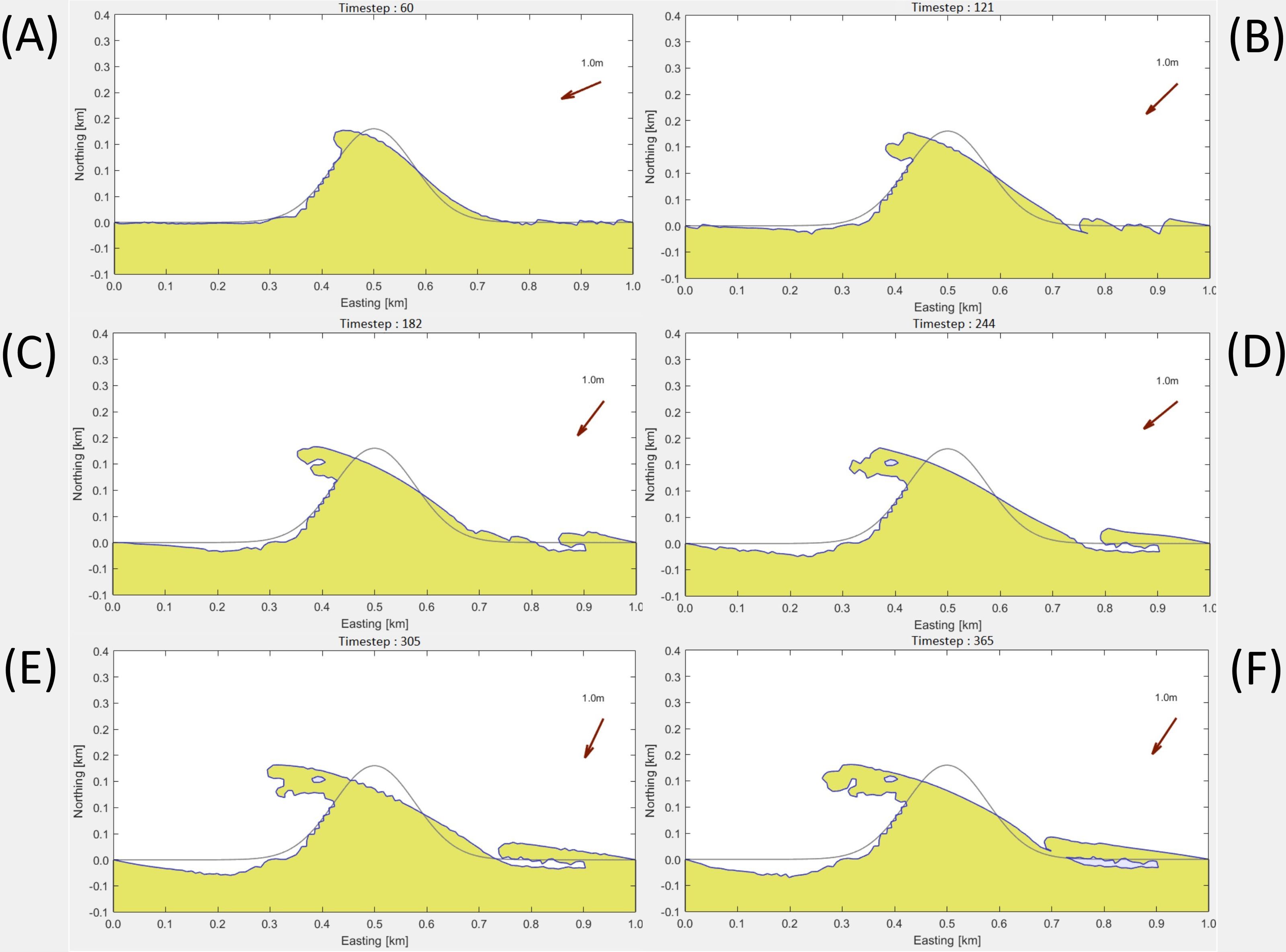
Figure 2. ShorelineS model output for the designed scenario at time steps 60, 121, 182, 244, 305, and 365, labelled as panel (A–F) respectively.

2.4 Data pre-processing

Raw data is often messy and unsuitable for direct use in ML models, requiring pre-processing to clean and convert it into a usable format. This step is essential for building reliable models, as data forms the foundation of ML. Raw data typically contains noise, outliers, and missing values, which can lead to unreliable predictions if not addressed (Thambawita et al., 2021). Consequently, before pre-processing, it is important to understand the data. In this section, we will first discuss the features and characteristics of the extracted data from the ShorelineS model, followed by the methods developed for pre-processing and preparing this data for our ML models. The most important part of ShorelineS model outputs for us is the x and y coordinates matrix. While these two matrixes (x and y) have the same size, since ShorelineS uses a flexible free-form string of grid points, this size is varying during the simulation based on the number of grid points in the shoreline vector at each time step.

In other words, the initial number of x and y coordinates might be 100 each, this number may increase or decrease throughout the simulation, though x and y will always have the same number of points at each timestep. As a result, the final x and y matrices will have dimensions of [maximum grid points during the simulation (e.g. 150) × number of outputs timesteps (e.g. 365)], but not all timesteps will used the maximum grid points, and “NaN” values filling the gaps.

If islands or lakes form during the simulation, their coordinates are added to the end of the main shoreline coordinates and separated by a “NaN” value. Each element in the x and y matrices has two indices: the row number, representing the coordinate, and the column number, representing the timestep.

$$x={\left[\begin{array}{ccccc}{x}_{0,0}& \cdots & x_{0,9}& \cdots & x_{0,366}\\ x_{1,0}& \cdots & x_{1,9}& \cdots & x_{1,366}\\ |& & |& & |\\ nan& \cdots & nan& \cdots & x_{49,366}\\ nan& \cdots & x_{50,9}& \cdots & x_{50,366}\\ nan& \cdots & x_{51,9}& \cdots & x_{51,366}\\ nan& \cdots & x_{52,9}& \cdots & x_{52,366}\\ nan& \cdots & |& \cdots & nan\\ nan& \cdots & x_{150,9}& \cdots & nan\end{array}\right]}_{150\times 366}y={\left[\begin{array}{ccccc}{y}_{0,0}& \cdots & y_{0,9}& \cdots & y_{0,366}\\ y_{1,0}& \cdots & y_{1,9}& \cdots & y_{1,366}\\ |& & |& & |\\ nan& \cdots & nan& \cdots & y_{49,366}\\ nan& \cdots & y_{50,9}& \cdots & y_{50,366}\\ nan& \cdots & y_{51,9}& \cdots & y_{51,366}\\ nan& \cdots & y_{52,9}& \cdots & y_{52,366}\\ nan& \cdots & |& \cdots & nan\\ nan& \cdots & y_{150,9}& \cdots & nan\end{array}\right]}_{150\times 366}$$

The complexities in ShorelineS output representation has the same problem of real-world shoreline observations, the number of coordinate points can vary, similar to the model’s output. When lakes or islands are present, the real-world shoreline can be represented like the model’s output, making this method applicable to sequential shoreline observations.

However, two issues need to be addressed before using the x and y matrices as input for ML models. First, “NaN” values cannot be processed by ML models. Masking them in the first layer won’t work, as “NaN” values would propagate through the coordinate vectors, resulting in an output filled with “NaN.” Yet, these “NaN” values are important for separating islands and lakes from the main shoreline. Second, the length of all x and y vectors must be consistent and only contain real values. Currently, “NaN” values are added to make each vector the same length as the longest output vector up to that timestep. To resolve these issues, we developed methods to reshape the original data into suitable formats for our ML models, which we will describe next.

2.4.1 Data interpolation

In this approach, we divide the x and y coordinate vectors into segments based on the location of “NaN” values, effectively breaking them into continuous sections. For example, an array like [1, 2, 3, NaN, 4, 5, NaN, 6, 7] is split into [1, 2, 3], [4, 5], and [6, 7]. Each segment is then proportionally resampled to a new length. After resampling, we record the length of each segment, which indicates the positions of the “NaN” values that separate islands or lakes from the main shoreline. The resampled sections are then concatenated into a single vector, which is used to train the ML model. After predictions are made, “NaN” values are restored into the coordinate vectors based on the recorded segment lengths. This process is illustrated in Figure 3.

Figure 3

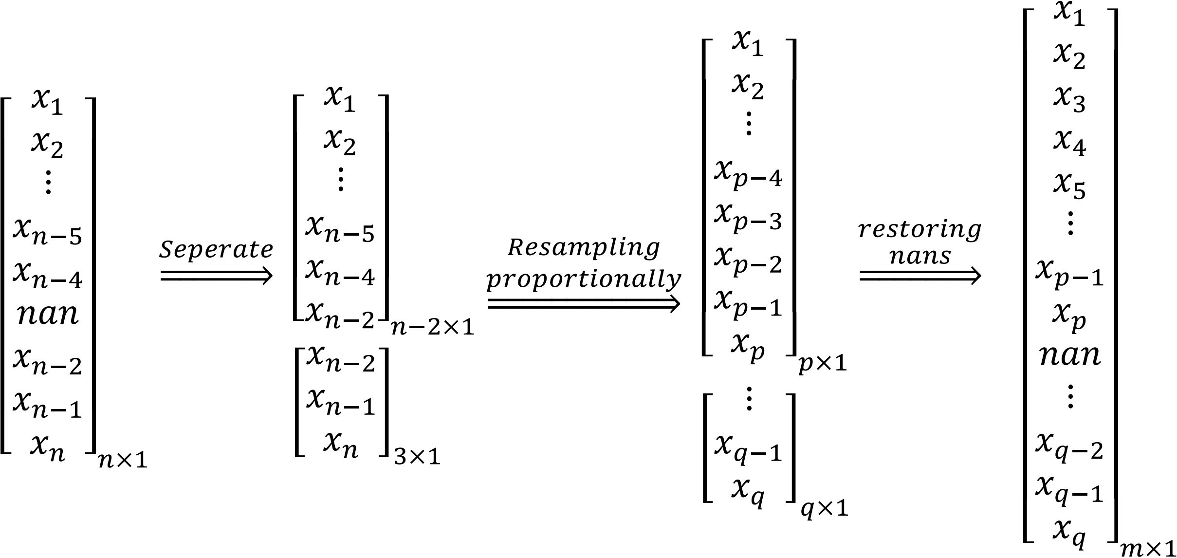
Figure 3. Process of “nan” value managing for the proposed interpolation method.

In this approach, interpolation transfers the data into a new fixed grid system. ShorelineS calculates shoreline positions on a free-form vector grid, but the grid length changes over time. To address this, we transform the grid to a constant length for all timesteps, allowing the ML models to identify spatial and temporal relationships more effectively. Determining the best grid size for this transformation is key. The ideal value is the length of the longest vector in the ShorelineS output. This minimizes changes in the grid system, reducing computational complexity and helping the ML models better capture spatial-temporal relationships. Although grid interpolation may cause slight shifts, this method ensures minimal data loss and optimized computational efficiency. Figure 4 illustrates how the x and y coordinates of grid point 75 shift over time, showing the grid’s movement that the ML models need to learn. Figure 5 compares the original and new grid systems for timestep 240, demonstrating minimal movement between grids using this interpolation method.

Figure 4

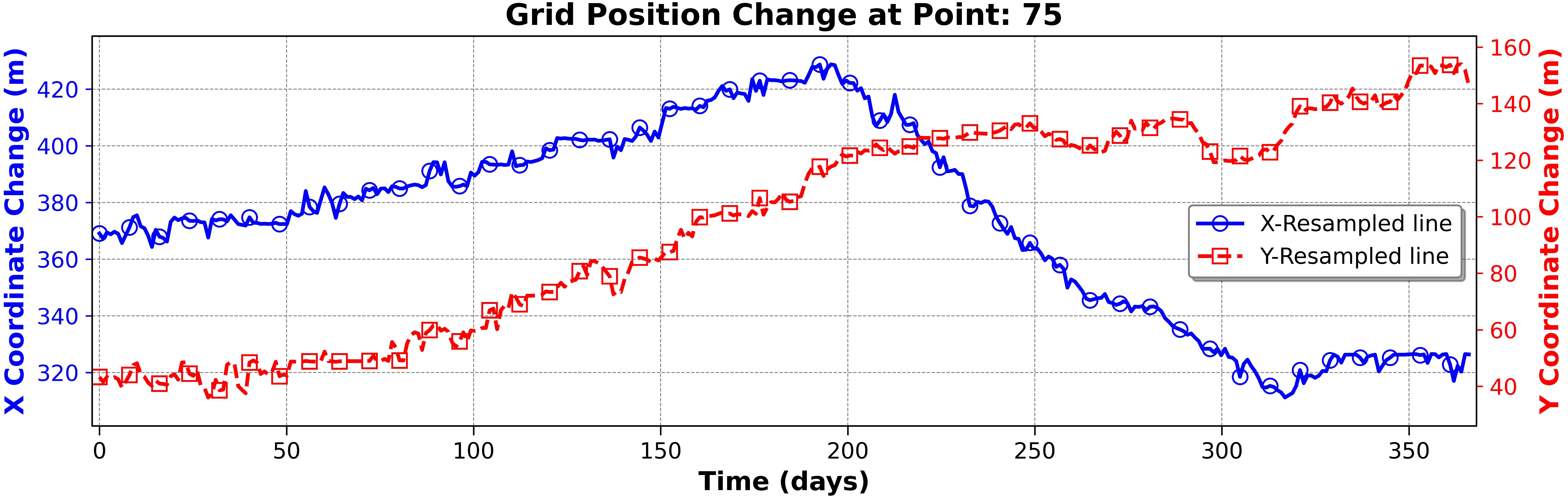
Figure 4. Grid position change for points 75 during progress in timesteps.

Figure 5

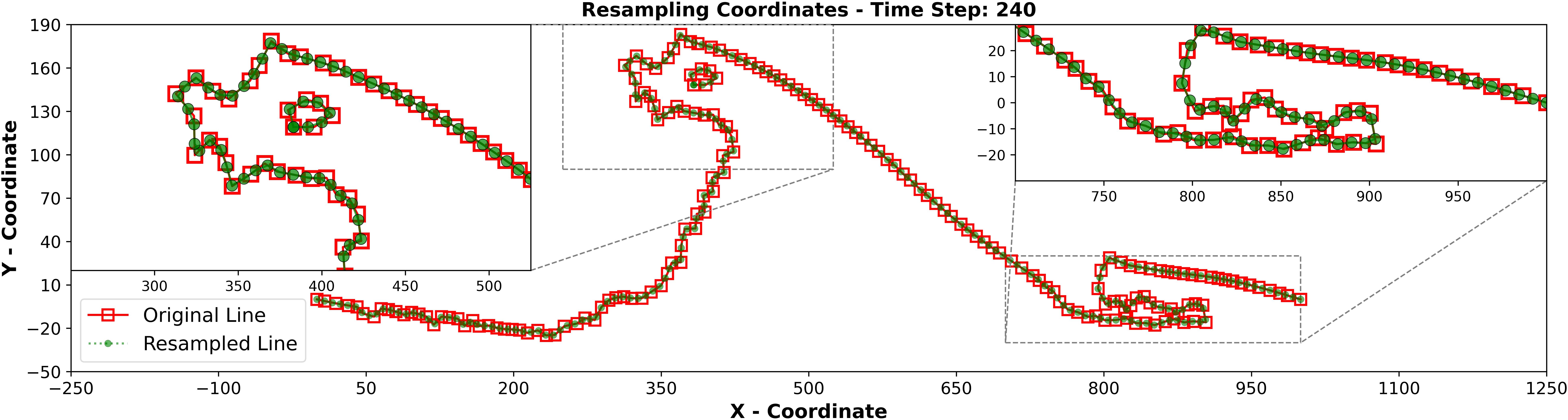
Figure 5. Comparison between original and new grid system (equally spaced) for timestep 240 using proposed interpolation method.

2.4.2 Optimal data representations for different ML models

ML models are highly sensitive to the shape and format of their input data, making it a critical factor in determining the model’s performance and accuracy. Therefore, careful attention must be given to the preparation and structure of the input data. In our case, we use sequential timesteps of [x] and [y] coordinate vectors, which can be arranged in various formats depending on the type of ML model being employed. This study explores several data representation methods, including One-row Array Representation (Row Vector), Two-row Array Representation, Image Data, and 2D Gridding Data. Detailed descriptions and the specific shapes of these representations are provided in the Supplementary Material of this article.

The shape and format of data should be chosen based on the machine learning architecture, the nature of the data, and the specific tools or frameworks (libraries) being used. For spatial coordinate data that varies over time, experimenting with different representations is essential for optimal performance. In this study, we evaluated various data representation methods to identify the most suitable options for the ML models employed. The selected representations, shown in bold in Table 1, have been chosen for further analysis. A comprehensive explanation of the selection process is provided in the Supplementary Material.

Table 1

Table 1. Appropriate data representational strategies for selected machine learning models.

2.4.3 Data splitting for training, validation and test

Ensuring reliable model performance is crucial for its future applications. While a trained model’s accuracy on training data is important, its performance on unseen test data truly matters. Overfitting is when a model performs exceptionally well on the training data but poorly on new data (James et al., 2013). This occurs because the model captures not just the underlying patterns in the data, but also its noise or random fluctuations. Hence, before starting with model training, we should always split the data into training, validation (cross-validation), and test sets. This ensures that we have a set of data to test the model’s performance on unseen data. Sequential data are time series and, in our case, which is a time series of coordinates, they have an inherent temporal ordering that needs to be preserved during splitting. This approach ensures that the training, validation, and test sets are representative of the data.

k-fold method is one of the best methods for cross-validation, but it is not ideal for our dataset. Because it randomly splits the data, which can cause data leakage and does not respect the time component of the data. Instead, it is recommended to use “TimeSeriesSplit” from the “scikit-learn” python library (Pedregosa et al., 2011). This method is a variation of k-fold cross-validation that takes time order into account. At each split, the train set remains fixed or increases in size, and the test set is a fixed size. In this method, the validation sets are non-overlapping and connected in terms of time. This means the data in the validation set for one fold will not appear in the validation set for another fold. For example, given a dataset of 10 points (labelled 1 through 10), we want to split it into 3 sets, with 4 data points for training and 2 for validation in each split. Using the “TimeSeriesSplit” method, the splits would look like this:

Original data = [1 2 3 4 5 6 7 8 9 10]

Train set 1 = [1 2 3 4] Validation set 1 = [5 6]

Train set 2 = [3 4 5 6] Validation set 2 = [7 8]

Train set 3 = [5 6 7 8] Validation set 3 = [9 10]

For the ShorelineS output with 365 timesteps, we reserved the last 5 for testing (which the model does not see) and used the remaining 360 for training and validation. We split the data into 58 segments, with each split containing 12 timesteps for training and 6 for validation. These values, 6 and 12, are hyperparameters that need to be optimized along with the model structure (e.g., number of layers and neurons). The optimization process was iterative, and we experimented with various combinations to find the best values. In real-world scenarios, these hyperparameters may reflect the underlying physics, such as seasonal cycles or tides. However, since our synthetic data does not involve cyclic events, the optimization process was more straightforward.

2.5 Models evaluation methods

Evaluating a machine learning model’s performance is a crucial step in developing reliable data-driven solutions. There are several methods that can be used to evaluate the performance of the ML models. In the following sections, we will discuss some of these methods that have been chosen or developed to evaluate the performance of used ML models in this study.

2.5.1 Prediction quality index

One of the common methods for the evaluation of meteorology models is the “Brier Skill Score” (BSS). This method has also been used in the evaluation of the coastal morphodynamics models by Brady and Sutherland (2001); van Rijn et al. (2003) and Sutherland et al. (2004). Sutherland et al. (2004) introduced Equation 1 to calculate the BSS for morphological models.

$\begin{array}{ll}BSS=1-\frac{<{(Y-X)}^2>}{<B-X^2>}& (1)\end{array}$

In the above formula, Y is a prediction, X is an observation, B is a baseline or initial shape of the shoreline and “< >“ is an arithmetic average. The BSS measures model performance by comparing its predictions to a baseline. A BSS of 1.0 indicates a perfect match between prediction and observation, while a BSS of 0 indicates the model performs the same as the baseline. Negative BSS values suggest the model performs worse than the baseline (Dastgheib, 2012); van Rijn et al. (2003) classified model performance based on BSS values is presented in Table 2.

Table 2

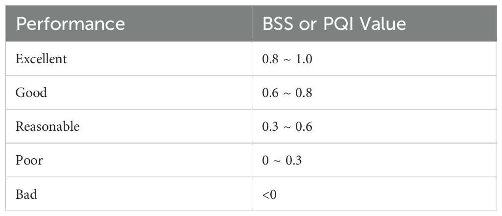
Table 2. Classification for model’s skill base on BSS or PQI value.

In this study, we work with data based on x and y coordinates. To evaluate the model’s skill, we developed the “Prediction Quality Index” (PQI), similar to the BSS. The PQI can be calculated using Equation 2.

$\begin{array}{ll}PQI=1-\frac{<{\text{Δ}}_{forcasts,X},{\text{Δ}}_{forcasts,Y}>}{<{\text{Δ}}_{refrence,X},{\text{Δ}}_{refrence,Y}>}& (2)\end{array}$

In Equation 2, ${\text{Δ}}_{forcasts,X} and {\text{Δ}}_{forcasts,Y}$ represent the averaged differences between predictions and actual observations for x and y coordinates, while ${\text{Δ}}_{refrence,X} and {\text{Δ}}_{refrence,Y}$ represent the differences between the baseline (initial shoreline) and actual observations. The PQI formula is based on the root-mean-squared error (RMSE), calculated as presented in Equations 3, 4.

$\begin{array}{ll}{\text{Δ}}_{forcasts}=\sqrt{\frac{{(p_1-a_1)}^2+\cdots +{(p_n-a_n)}^2}{n}}& (3)\end{array}$

$\begin{array}{ll}{\text{Δ}}_{refrence}=\sqrt{\frac{{(p_1-i)}^2+\cdots +{(p_n-i)}^2}{n}}& (4)\end{array}$

In the formulas above, “p” represents the predicted value, “a” is the actual observed value, “i” is the initial shoreline position, and “n” is the number of observations. The PQI calculates the ratio between the divergence of predicted and observed data and the divergence of the observed data from its initial position. This index is categorized similarly to the BSS into five performance levels, as shown in Table 2. It is important to note that the PQI should not be used to compare the performance of two models. Instead, it is intended to assess a model’s accuracy at a specific timestep, based on the changes that have occurred up to that point. This allows for more acceptable errors during periods of substantial change.

2.5.2 CC, RMSE and MAE metrics

Correlation Coefficient (CC), Root Mean Squared Error (RMSE) and Mean Absolute Error (MAE) are commonly used metrics for evaluating the performance of predictive models. In the following section, we briefly introduce these metrics. These metrics have been calculated for all 365-time steps across all the studied machine learning models and will be compared in the following sections. It is important to note that for models using matrix data instead of coordinate data, the metric results will not be reported separately for the x and y coordinates. Instead, the metric values will be averaged across the entire surface of the data, encompassing all values represented in the predicted result as a matrix.

The CC measures the linear relationship between the predicted values and the observed (actual) values and can be calculated from Equation 5. CC can be between +1 and -1 (Solomatine, 2023).

● +1: Perfect positive linear relationship

● 0: No linear relationship

● -1: Perfect negative linear relationship

$\begin{array}{ll}CC=\frac{{\sum }_{i=1}^n(x_i-\overline{x})(y_i-\overline{y})}{\sqrt{{\sum }_{i=1}^n{(x_i-\overline{x})}^2{\sum }_{i=1}^n{(y_i-\overline{y})}^2}}& (5)\end{array}$

In Equation 5, x_i and y_i are data points, and $\overline{x}$ and $\overline{x}$ are the means of x (predicted values) and y (observed values) respectively.

RMSE is the average difference between the predicted values and the observed values. This metric helps to determine how close a model’s predictions are to the real outcomes. The lower the RMSE, the better the model’s predictions and this metric penalizes errors at high values. This metric can be calculated from Equation 3 (Solomatine, 2023).

MAE is the average of the absolute differences between the predicted and observed values and can be calculated from Equation 6. This metric does not penalize high errors (Solomatine, 2023).

$\begin{array}{ll}MAE=\frac{1}{n}\sum |y_i-{\widehat{y}}_i|& (6)\end{array}$

In the above formula, $y_i$ is the observed value, ${\widehat{y}}_i$ is the predicted value, and n is the number of observations.

2.6 Machine learning models preparation and training

For optimal training of ML models and to achieve the best possible results, certain options and settings must be configured. In this section, we describe the selected options, and their corresponding settings used in the ML models for this study. Unless stated otherwise, these settings remained unchanged throughout the analysis.

To train all the mentioned ML models that work directly with coordinate data, we apply normalization. Normalization, specifically Min-Max Scaling, transforms features to a common scale, typically within the range [0, 1]. This transformation is essential because certain algorithms, particularly those relying on distance calculations or gradient-based optimization, may experience numerical instabilities or longer training times if the feature scales vary significantly (Mirtaheri and Shahbazian, 2022).

In supervised learning, the goal is to adjust model parameters, such as neural network weights, so predictions closely match observed values. This is achieved by minimizing a loss function, which quantifies the difference between predicted and actual values. An optimizer efficiently finds the global minimum of this function. In this study, we used Adaptive Moment Estimation (ADAM), which combines the strengths of the Adaptive Gradient Algorithm (AdaGrad) and Root Mean Square Propagation (RMSProp) (Mirtaheri and Shahbazian, 2022). ADAM is computationally efficient, memory-friendly, and well-suited for large datasets and complex models, making it an ideal choice for our ML models.

The learning rate is a key hyperparameter that controls the step size during each iteration as the model minimizes the loss function. In gradient descent (here, ADAM), it determines how large each update should be in the direction of the negative gradient. An appropriate learning rate ensures efficient convergence: if too high, the model may overshoot the minimum, causing oscillations or divergence; if too low, convergence slows, requiring more iterations. A slightly higher learning rate can also help escape local minima and find a better or global minimum (Mirtaheri and Shahbazian, 2022). In this study, the learning rate decays exponentially rather than remaining fixed. It starts at 0.001 and decreases over time, multiplying by a decay rate of 0.9 every 100 steps. This approach accelerates early convergence while later refining training as the model nears the optimal solution.

An epoch is a full cycle in which the entire training dataset passes forward and backward through the model. During each epoch, the model makes predictions, calculates the difference between predicted and actual values using a loss function, and updates its weights through an optimization algorithm to minimize the loss. The number of epochs is crucial for training duration. More epochs can improve learning and accuracy but also increase computational costs. Some models require more epochs to fully converge, while others reach a point where additional training offers little or no improvement (Mirtaheri and Shahbazian, 2022). Training for too many epochs can cause overfitting, where the model performs well on training data but fails to generalize to new data. This occurs when the model memorizes the training data instead of learning meaningful patterns. A validation dataset is typically used to assess performance at the end of each epoch. If validation performance declines while training performance improves, overfitting may be occurring (Solomatine, 2023).

To prevent this, early stopping can halt training when validation performance deteriorates. This method monitors a chosen metric, typically validation loss, and stops training once improvement ceases. A patience parameter defines how many epochs to wait before stopping after no further progress is observed. Instead of training for a fixed, large number of epochs—which is computationally expensive and time-consuming—early stopping allows training to end sooner while maintaining efficiency. It also ensures that the best-performing model, with the lowest validation loss, is saved (Brownlee, 2018). In this study, we used early stopping to prevent overfitting and optimize model performance.

Grid Search is a hyperparameter tuning method used to optimize an ML model’s structure and settings. Since hyperparameters significantly impact performance, this study focused on tuning key ones: the number of layers, neurons per layer, activation function, and initial learning rate. The process starts by defining a subset of the hyperparameter space, systematically testing all possible combinations, and evaluating performance on the validation set. The best-performing set is selected, with minor adjustments made for structural consistency before finalizing the configuration (Brownlee, 2018).

3 Results

In this section, we present and compare only the most significant final results from our selected ML models, focusing on cases with noteworthy points of discussion for the sake of brevity. Additionally, at the end of this section, we compare the training and prediction times of each ML model with our baseline model. It is important to note that results not discussed here are provided in the Supplementary Materials of this paper.

3.1 DNN model performance

In this section, we will evaluate the performance of the DNN model when data from proposed interpolation method is fed into it.

Based on the methodology outlined in the previous section, the optimal DNN model consists of three hidden layers with the “ReLU” activation function, a “Sigmoid” activation function in the output layer, and an initial learning rate of 0.001.The changes in accuracy and loss over time for both the training and validation datasets during the DNN model training process are provided in the Supplementary Materials. Figure 6 illustrates the results of the PQI in panel (A) and Comparison of the MAE for X and Y coordinates at each timestep in panel (B). From this figure we can see, initially, the ratio of prediction error to the amount of change is low, but this improves over time. A low PQI value in the early timesteps does not necessarily indicate poor model performance or high error (see Figure 6B). It can also suggest that the prediction error is small, especially when the overall change in the model is minimal. However, this indicates that the model’s performance in the early timesteps is less reliable. From this figure, we can also observe a sudden drop in the PQI value at certain time steps, such as 135, 212, and 336. To ensure that this is not due to a miscalculation of the PQI value or a minor error in prediction—where the magnitude of change in the model is significantly smaller than the error as described above—we have plotted the MAE values for the x and y coordinates across all time steps in Figure 6B. At these exact time steps, a sudden increase in the MAE is evident. Therefore, it is necessary to investigate these anomalies further and determine what is occurring at those time steps.

Figure 6

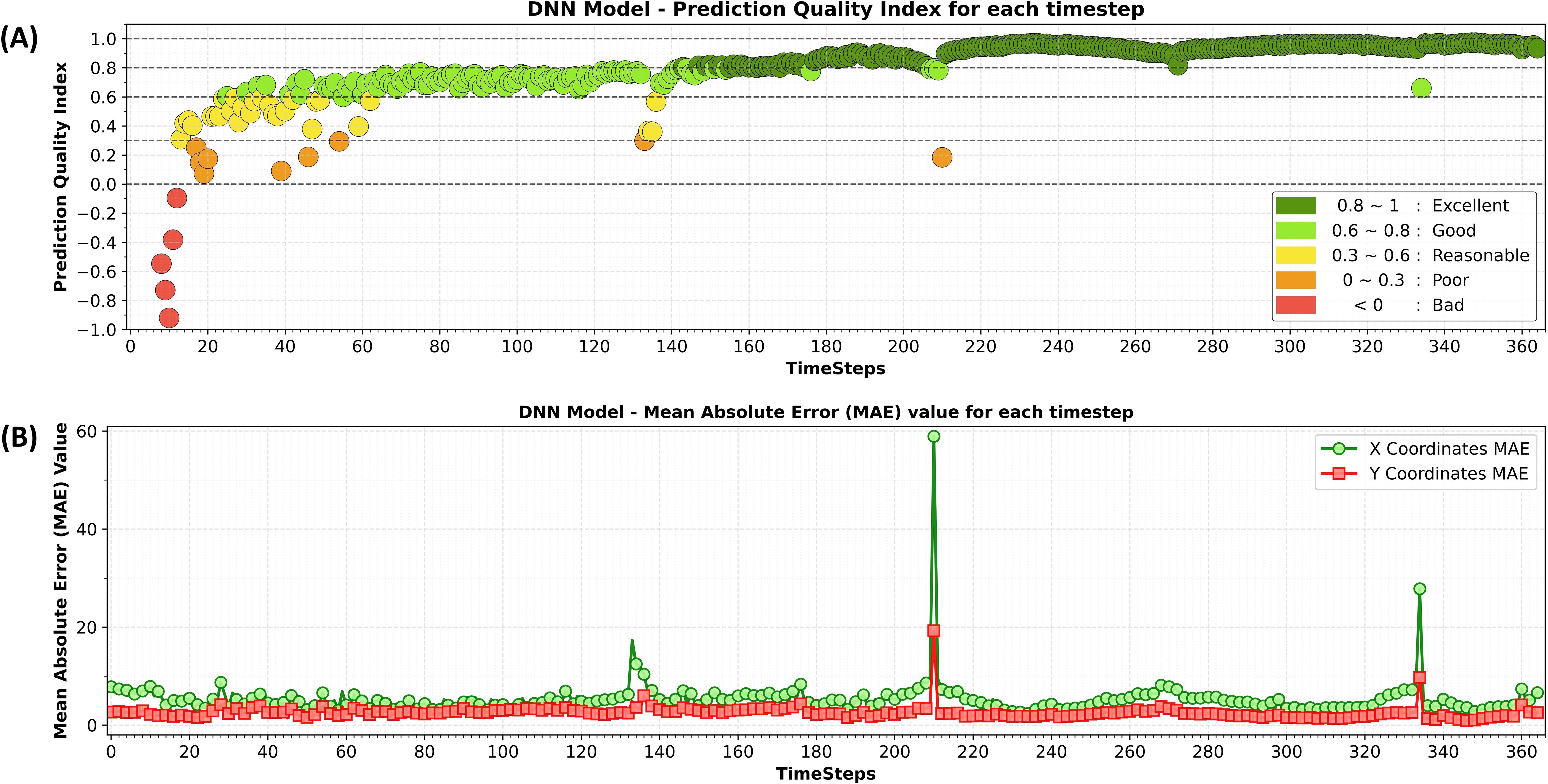
Figure 6. PQI at each timestep, labelled as panel (A) and comparison of the Mean Absolute Error (MAE) for X and Y coordinates at each timestep, labelled as panel (B).

As shown in Figure 6, there are noticeable dips in model performance at timesteps 135, 212, and 336. Figure 7 helps explain these dips by tracking grid position changes for point 203 across all timesteps as an example. This figure reveals sudden shifts in grid positions at these specific times, caused by the formation of lakes in the numerical model as shown in Figure 8A–C. When the lakes form, their coordinates are moved to the end of the coordinate vector, which forces the new grid system to create jumps in the x and y coordinates (Figure 7). These inconsistencies disrupt the training process and complicate the ML model’s task, resulting in increased errors and reduced model performance. The final results from the trained DNN model at timesteps 60, 120, 180, 240, 300, and 365 are provided in the Supplementary Materials.

Figure 7

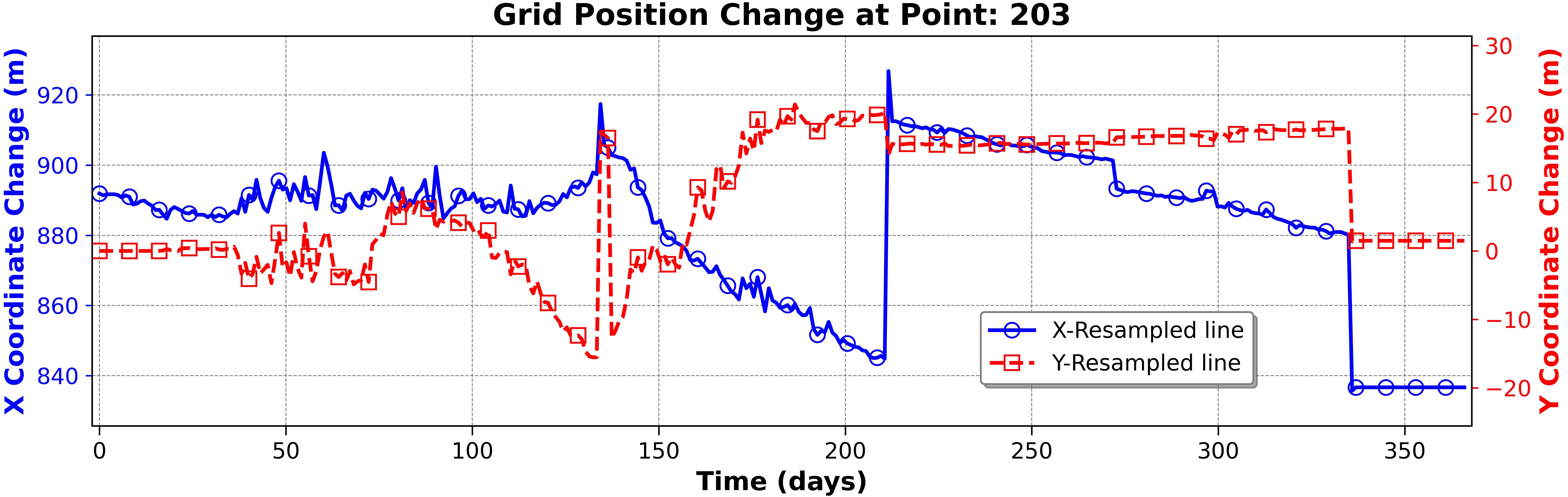
Figure 7. Grid position changes (movements or jumps) for grid point 203 in the X and Y coordinates over time.

Figure 8

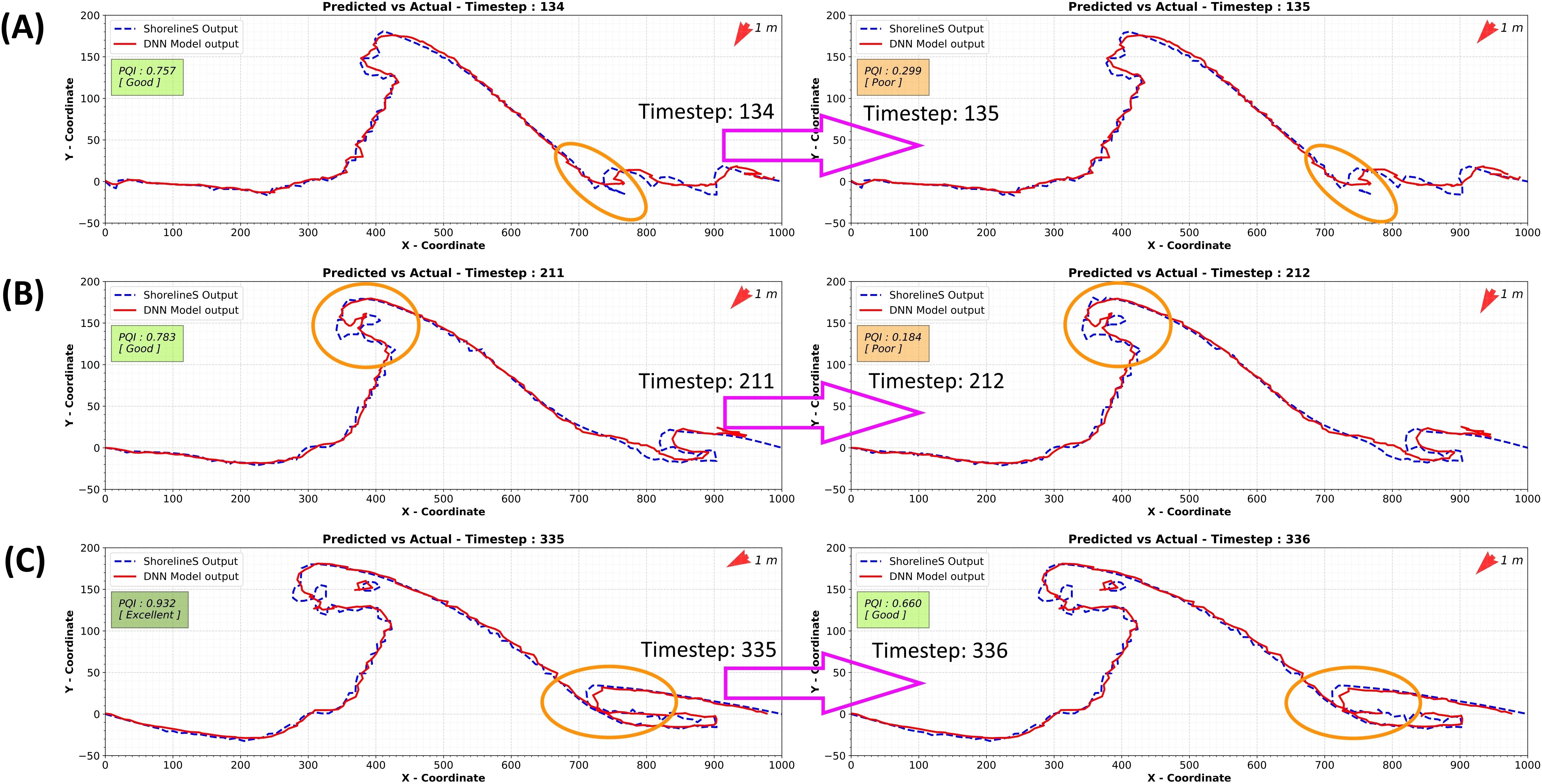
Figure 8. Creation of lakes in the ShorelineS model and the ML model: Reasons for jumps at timesteps 135, 212, and 336. Panel (A) timestep134 to 135; Panel (B) timestep 211 to 212; Panel (C) timestep 335 to 336.

3.2 CNN model performance

In this part, we will discuss the results of the CNN model, trained on, “Two-Row data” and “Image outputs” data. For both CNN models, we also employed the Early Stopping method mentioned before.

3.2.1 CNN performance on two rows data

Based on the grid search analysis, the best CNN model for our Two-Row data array consists of four 1-dimensional convolutional layers with 128, 64, 32, and 16 features in each layer, respectively, all using the “ReLU” activation function. This is followed by a Flatten layer that reshapes the multi-dimensional input into a single long vector. This layer is typically used when transitioning from a convolutional layer to a dense layer within a network. Subsequently, a Dense layer with a “Sigmoid” activation function is added to the structure; this fully connected layer produces the desired output. Finally, a Reshape layer is incorporated to adjust the network’s results to match the shape of the input data. The PQI performance of the model trained on this data structure (Figure 9) shows an improvement compared to previous results. While the final outcomes for this ML model are considered acceptable, sudden jumps in PQI values still occur due to the formation of islands and the resulting shifts in shoreline position coordinates, as discussed in the previous section. For brevity, the model’s performance and the alignment between true and predicted results are provided in the Supplementary Materials.

Figure 9

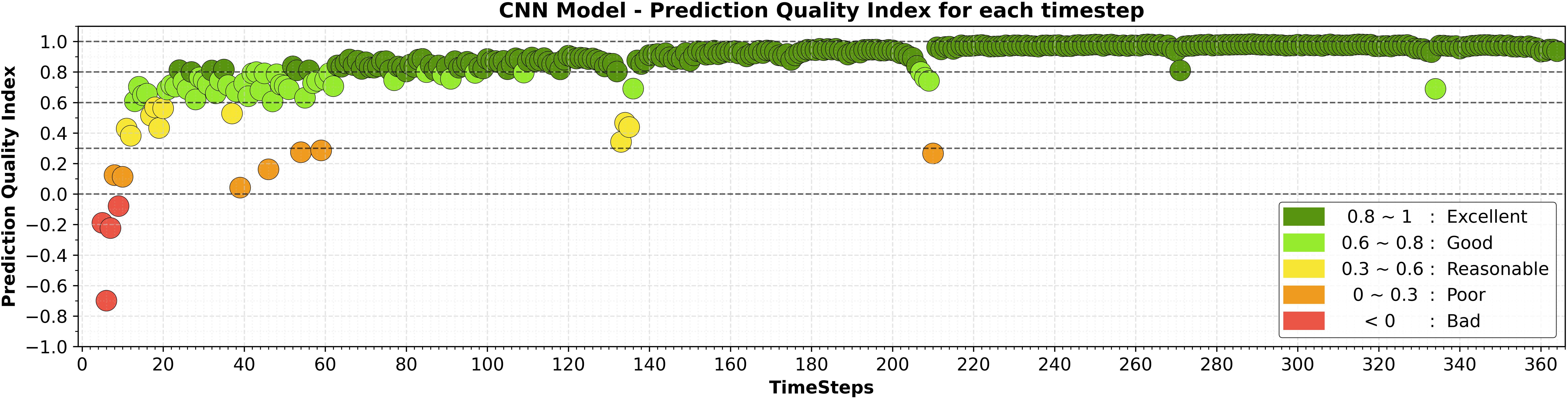
Figure 9. PQI for each timestep for CNN model trained on Two-row data array.

3.2.2 CNN performance on image data

The optimal 2-dimensional CNN model for our Image data includes four 2-dimensional convolutional layers. These layers generate feature maps with 40, 20, 10, and 1 channels, respectively. The first three layers employ the “ReLU” activation function, while the last layer uses the “Sigmoid” activation function. The model maintains the spatial dimensions, equivalent to the input image size across all convolutional layers to preserve the spatial information of the input data. This can be particularly useful for tasks where the spatial structure of the input is crucial. The final results for ML model trained on image data are significantly better compared to using two rows of data as input. While this approach effectively eliminates sudden jumps in PQI values, leading to a substantial improvement in the final outcomes, it is not without flaws. In some cases, the model may learn and reproduce features from the image that are unrelated to the shoreline evolution. This issue occurred during one of our tests using a CNN model to predict shoreline evolution for a test case. In this test case, the numerical model incorrectly plotted the shoreline position at one timestep by adding an extra line. Consequently, this error was learned and replicated exactly in the CNN prediction results, as illustrated in Figure 10B.

Figure 10

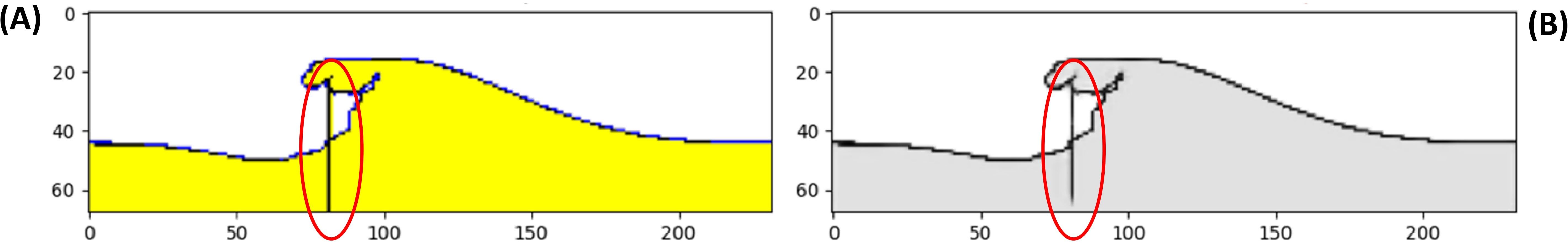
Figure 10. Recreation of plotting error in CNN model output. Panel (A) numerical model output; Panel (B) CNN model output.

3.3 LSTM model performance

3.3.1 LSTM performance on one row data

In this study, while we attempt to train an LSTM model on One-Row data, we observed no improvement during the training process. Consequently, the training was automatically stopped due to the “Early Stopping” option. The underlying issue was that the LSTM model could not effectively learn from the One-Row data structure ($[x_1,x_2,\cdots ,x_{n-1},x_n,y_1,y_2,\cdots ,y_{n-1},y_n]$), as the model inherently expects sequential input. The positioning of the y array after the x array disrupts this expected sequence, confusing the model during training.

After identifying the best possible structure for the LSTM model using Two-Row data (next section), we applied this optimal structure to the LSTM model with One-Row data. We also removed the early stopping from this model and trained it for the same number of epochs as the Two-Row data model to observe the final results. Although we cannot consider the outcomes of this model as valid, we reported them in the Supplementary Material for the sake of transparency.

3.3.2 LSTM performance on two rows data

The optimal LSTM model for our Two-Row data includes four LSTM layers, each having 10 features. After the data is processed through these recurrent layers, the model transitions to a fully connected Dense layer. This Dense layer outputs sequences including 224 units, each with 2 features, thus replicating the same data format that was the input of the model. This transitional layer uses a “Sigmoid” activation function.

The PQI and the comparison between observed and predicted results from both LSTM models showed neither significant agreement nor an acceptable range based on the definition of PQI and error values. For clarity, these results are presented in the Supplementary Material of this paper. It is important to note that the first approach (using One-Row data) was unsuccessful, and the second approach (using Two-Row data) did not produce promising results, particularly in modelling the spit head and lakes compared to other ML models. Additionally, training these models was time-consuming, especially when considering their performance relative to other tested models. The training time for each model is discussed further in another section.

3.4 ConvLSTM model performance

This section presents the performance of ConvLSTM models on three data types: Two-Row array data, Image data and 2D Gridded data.

3.4.1 ConvLSTM performance on two rows data

The optimal structure, derived from the grid search results and slightly manually enhanced for structural consistency, consists of a model with three ConvLSTM2D layers. Each layer has 100 feature maps or channels and uses a “Tanh” activation function. The “TimeDistributed” wrapper is also used to apply a layer to every temporal slice of an input. When we use the “TimeDistributed” wrapper, it allows us to apply a specific layer to every temporal slice (or timestep) of an input sequence. Each timestep is processed independently, effectively enabling simultaneous calculations for all timesteps. It ensures that the same operation (or layer) is applied in the same way across every timestep in the sequence. It should be noted that, as with all other models, this model also employs the “Early Stopping” method to prevent overfitting and ensure optimal performance.

The final results of the trained ConvLSTM model while using two rows data representation is presented in the Supplementary Material of this article. As evident, the model’s understanding of the shoreline evolution process is not particularly accurate for lakes and islands. This inaccuracy may stem from the LSTM component of the ConvLSTM model, as we observed similar issues with pure LSTM models previously. However, the process of evolution of the main shoreline is well-understood and represented accurately.

3.4.2 ConvLSTM performance on image data

The optimal structure, derived from the grid search results and enhanced manually for structural consistency for our ConvLSTM model working on image data, includes nine ConvLSTM2D layers interspersed with Batch Normalization and Dropout layers. All these layers use the “Tanh” activation function, except for the final Conv3D layer, which employs a “Sigmoid” activation function. The number of filters for these layers is as follows: 64, 32, 16, 8, 1, 8, 16, 32, and 64 for the ConvLSTM2D layers, and 1 for the Conv3D layer. The changes in model accuracy and loss as well as the PQI performance of the mode and the final predicted results are reported in the Supplementary Material of this paper. Overall, the performance of the model trained on image data has improved compared to the previous approach. However, the model remains sensitive to defective input images, which can result in inaccurate predictions as we discussed before.

3.4.3 ConvLSTM performance on 2D gridded data

In this section, we will evaluate the model’s performance using “2D Gridded Data”. We will use the optimized ConvLSTM model from the previous section (ConvLSTM for Image Data) as a reference for this evaluation. The PQI in this case demonstrates strong model performance. However, at the early timesteps, some predictions exhibit lower PQI values. This occurs because the changes in the model at these timesteps are relatively small compared to the prediction error. The accuracy and loss plots for the training and validation datasets during the ConvLSTM model training with “2D Gridded Data”, along with the PQI plot, are provided in the Supplementary Material.

The comparison between the final replicated and predicted results of the ConvLSTM model in this case and the actual values (output of the ShorelineS model) is illustrated in Figure 11A–F. As can be seen, the model’s performance is very promising and reliable. It is important to note that the smallest change that can be predicted is determined by the resolution used to convert the input data into 2D gridded data. In this case, a resolution of 2 meters was used, meaning the smallest detectable change in shoreline position with our ML model is 2 meters.

Figure 11

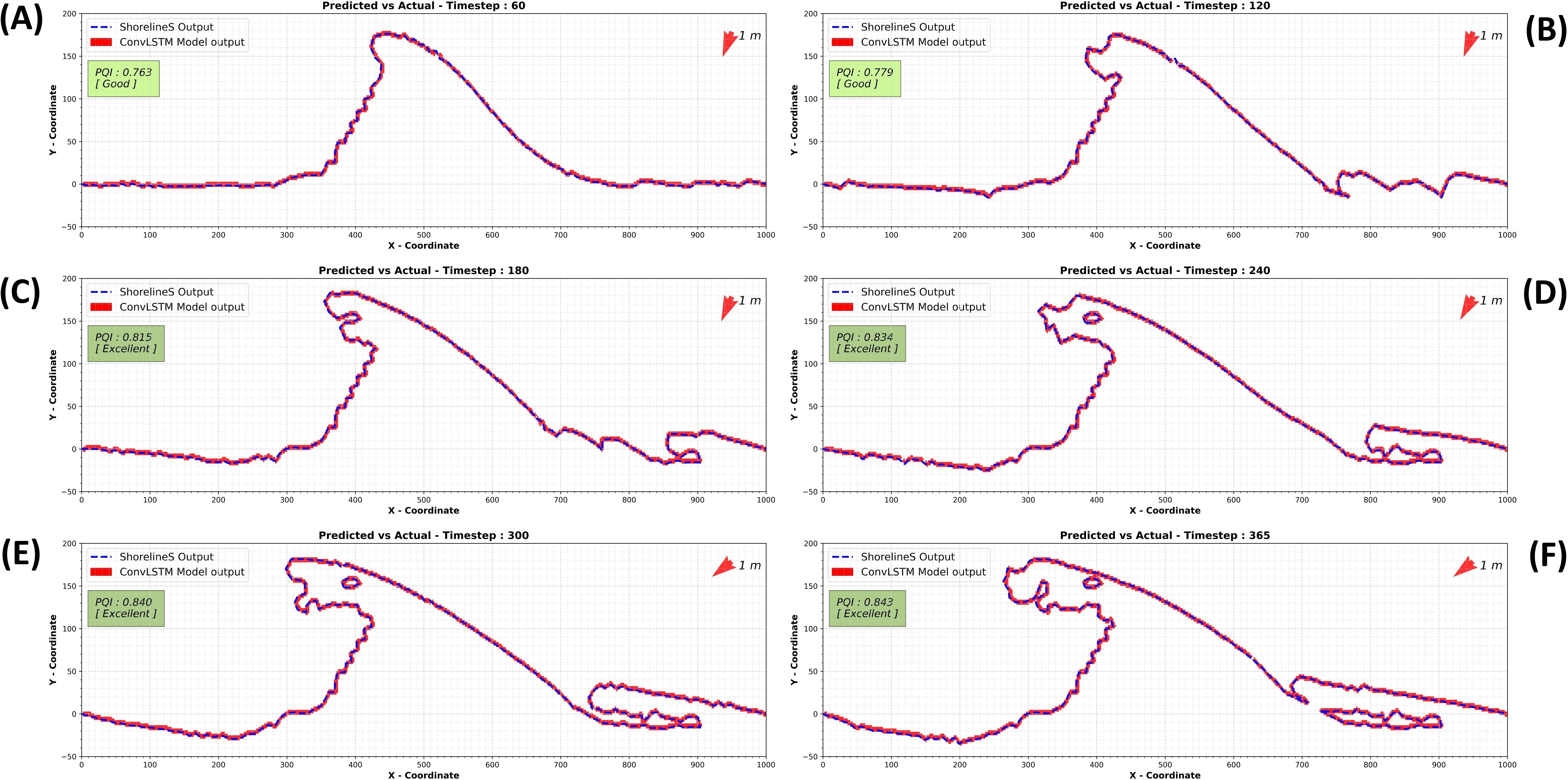
Figure 11. Replication of shoreline evolution and its prediction by the trained ConvLSTM model at timesteps 60 (A), 120 (B), 180 (C), 240 (D), 300 (E), and 365 (F) on 2D gridded data.

3.5 Comparing ML models and methods

In previous sections, we evaluated the performance of different ML models on various data structures. Here, we compare the training time and output generation time for these algorithms. By “generation”, we mean the time taken to produce prediction results for all 365 timesteps (for both seen and unseen data) after training.

Except for models using Image and 2D Gridded data, which require more memory, all models were trained on a standard personal computer. For consistency, however, we trained and generated outputs for all models using Google Colaboratory’s A2 accelerator-optimized machine with NVIDIA Tesla A100 GPUs. The system specifications are as follows (Google Co, 2023):

● GPU: 1 GPU - NVIDIA Tesla A100

● Available vCPUs: 12 vCPUs

● Local SSD supported: Yes

● GPU memory: 40 GB HBM2

● Available memory: 85 GB

For the ShorelineS model, it was not possible to run it on Google Colaboratory, so we ran it on a laptop with the following system specifications:

● Model: HP ProBook 450 G8 Notebook PC

● Memory: 8GB DDR4

● Graphics Card: Intel(R) Iris(R) Xe Graphics

● Processor: Intel Core i5-1135G7

● Storage: Kingston 500GB SSD

● Operating System: Windows 10 Enterprise

The recorded times for running ShorelineS and training all ML models are reported in Table 3. In ShorelineS, results are saved while calculating each timestep, so we report this as “training duration” in this table. We can see that generally, as ML models become more complicated, the required time for training them increases. It is worth noting that some models, while taking considerable training time, did not deliver acceptable performance, such as the LSTM models. Models working on Matrix data typically require more training time due to the volume of data within the matrix, but their final results are generally superior to other models.

Table 3

Table 3. Duration of training and output generation for ShorelineS and various ML models.

To enable a more detailed comparison of model performance, the exact metrics for timesteps 60, 120, 180, 240, 300, and 365 are also investigated (reported in the Supplementary Material). Models in Table 3 (and table of calculated metrics in the Supplementary Material) can be categorized into two groups: those that work with coordinate data (models number 2, 3, 5, 6, and 7) and those that work with matrix data (models number 4, 8, and 9). In the first group, training times are fairly consistent across models, except for the LSTM models, which took significantly longer. However, both LSTM models performed poorly for shoreline prediction. The LSTM with “One-Row Data” produced unreliable results, while the “Two-Row Data” LSTM required long training times and delivered less accurate results compared to other models. Among the models processing coordinate data, the CNN model performed best, followed by ConvLSTM with “Two-Row Data”, DNN with “Two-Row Data”, and DNN with “One-Row Data”.

For the second group of models (using matrix data), based solely on the raw metrics and ignoring factors like training time, possible image defects, and resolution (the smallest detectable change), the CNN model using “Image Data” performed best, followed by ConvLSTM with “Image Data” and ConvLSTM with “2D Gridded Data”.

To make an informed model selection, we assigned scores from 0 to 5 to each model based on various constraints. This scoring allows for a comprehensive comparison to identify the best model for the designed scenario. The criteria and scoring are as follows:

● Training time: Models lose points with increasing training time. The most efficient model receives a score of 5.

● Image defects: If there’s a possibility of image defects, the model is penalized with 0. If not, it receives a score of 5.

● Control over prediction details: Models gain more points with increased control over prediction details.

● Accuracy: Models with higher accuracy earn more points.

For the models using matrix data, the final result of scoring and comparison is shown in Table 4. From this table, it becomes evident that the ConvLSTM model, when used with “2D Gridded data”, is the optimal choice for our scenario.

Table 4

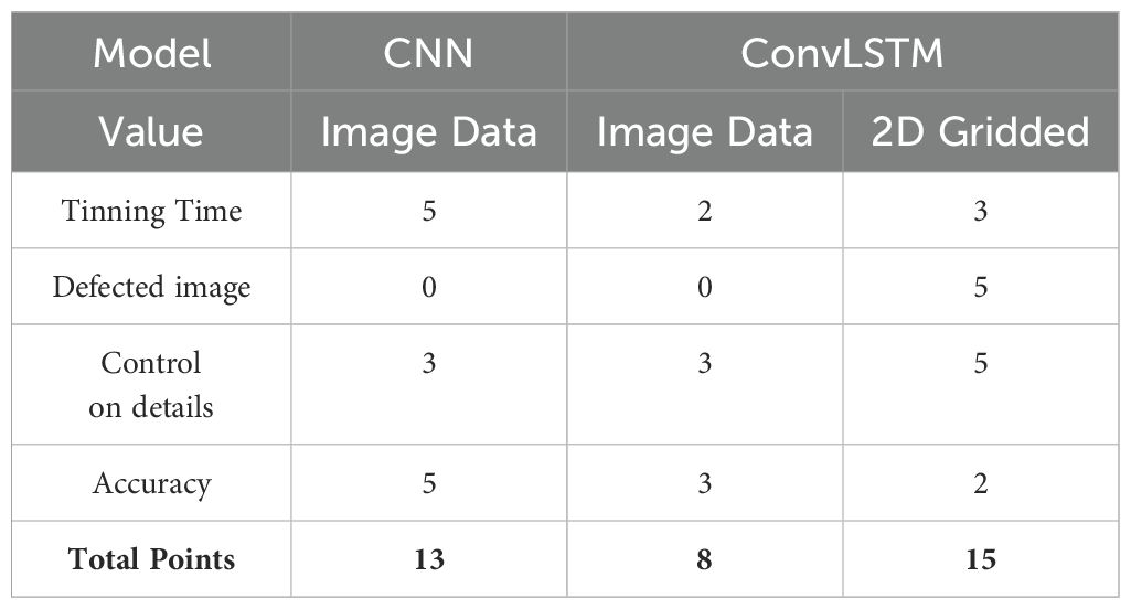
Table 4. Scoring models based on defined constraints.

4 Using ML for probabilistic prediction of shoreline changes

In this section, we build on the findings of the previous section to explore how our best ML model can be used as a probabilistic tool for studying and addressing uncertainties in shoreline position modelling.

Shoreline development and final positions are influenced by various uncertainties, one of the main sources being the variability in wave directions during simulations (Kamphuis, 2010). In process-based models like ShorelineS, when a wave climate is used as input a chronologically random wave height and direction are generated as model forcing. The implementation of different time series generated from the same wave climate can change the evolutionary path of the coastline.

For example, Figure 12A, shows the evolution of an initial Gaussian hump-shaped shoreline after one year of simulation for two runs with identical inputs. Despite using the same wave height and directional spreading, the model internally generates different wave direction sequences based on the mean direction and spreading factor (Figure 12B), resulting in different final shoreline positions.

Figure 12

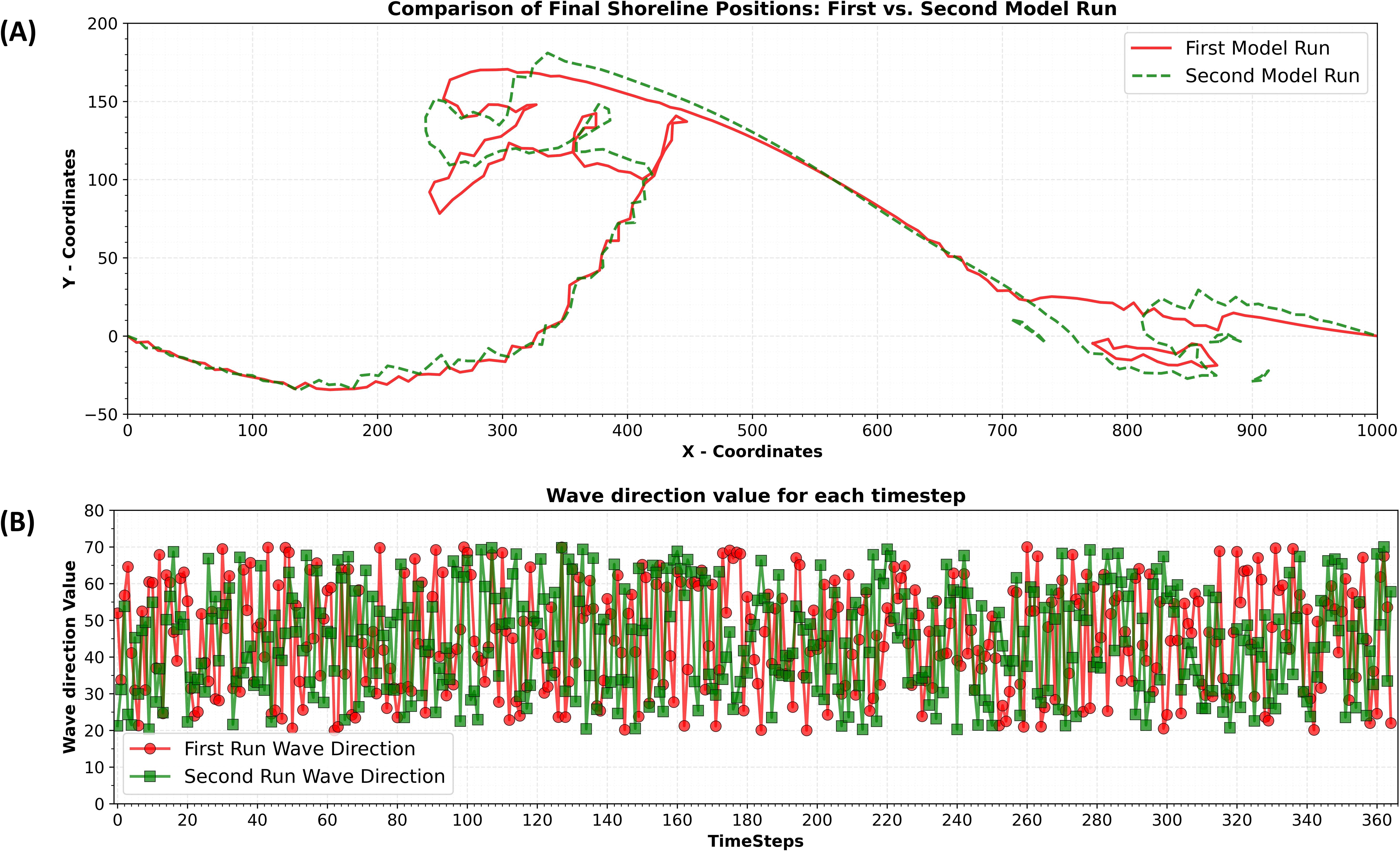
Figure 12. Top Panel: Comparison of the final position of the shoreline after running the ShorelineS numerical model two times, labelled as (A); Bottom Panel: Comparison of wave directions between the first and second ShorelineS model runs, labelled as (B).

To further investigate the effect of the spreading factor on the final shoreline position, we ran ShorelineS 1000 times and recorded the shoreline position at the end of each simulation, as shown in Figure 13A. This value balances capturing the model’s full variability and maintaining a feasible computational cost. In Monte Carlo approaches, increasing the number of runs reduces sampling error and improves statistical reliability. We observed that, beyond approximately 1,000 runs, improvements became marginal, while fewer runs risked missing important variations. Therefore, 1,000 runs provide a sufficiently large sample for robust statistical estimates while keeping computational costs manageable. Using this data, we generated a probability plot of the outputs. In this plot, each time a shoreline passes through a pixel, that pixel’s value increases by 1, starting from an initial value of 0. Each pixel represents an area of 2×2 meters. We repeated this process for all 1000 final results. The probability plot is then created by dividing each pixel’s value by the maximum pixel value within the domain (Figure 13B).

Figure 13

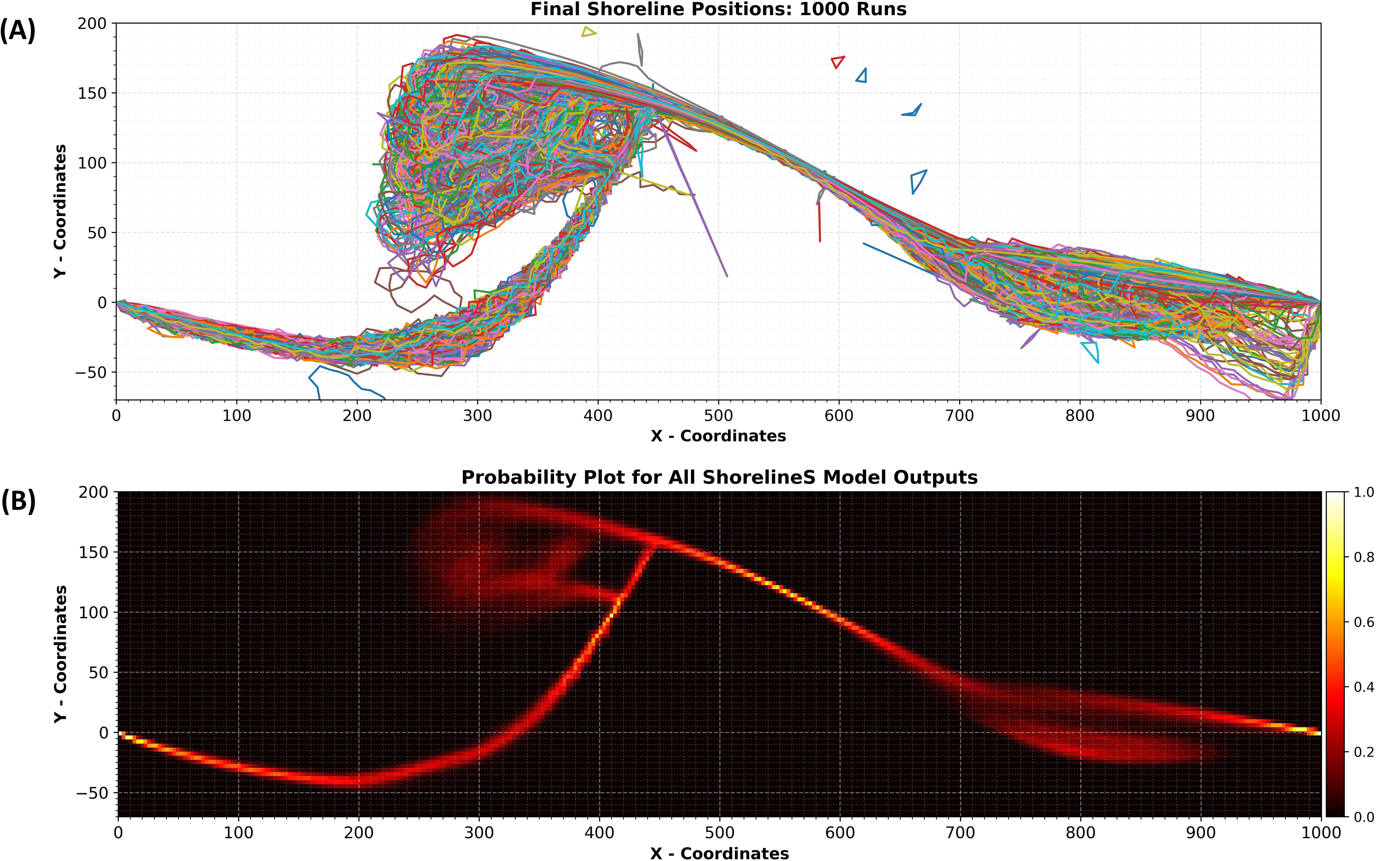
Figure 13. Top Panel: All shoreline positions at final timestep for 1000 ShorelineS model runs, labelled as (A); Bottom Panel: Probability plot for all shoreline positions at final timestep for 1000 ShorelineS model runs, labelled as (B).

In previous sections, we examined ML models that effectively learn shoreline evolution and demonstrated their ability to recreate shoreline positions at the end of simulations. Now, we aim to use these models to manage uncertainties in numerical modelling. Specifically, we will use our best-performing model from the previous section, the ConvLSTM model with 2D gridded data, to predict shoreline changes under different wave directions in a probabilistic way.

To do this, we introduce a simple method called the “Adaptive Model Selector”. While it’s inspired by the ensemble model (Zhou, 2012) concept, which typically combines multiple models to improve prediction accuracy, however our method works somewhat differently. Instead of combining models, it selects and combines predictions from pre-trained models, each trained for a specific wave direction with no directional spreading. By using a Monte Carlo method to generate wave directions timeseries, the adaptive model selects the most suitable models at each time step to make prediction.

We combine the Monte Carlo simulation method with the “Adaptive Model Selector” to predict 1000 possible shoreline positions and estimate the probability of shoreline existence at various points on a 2D grid. To achieve this, we generate 11 sets of synthetic gridded data, each representing a different shoreline evolution scenario using the ShorelineS numerical model. For each scenario, we train a ConvLSTM model with the same structure as before. These 11 models, each trained for a specific wave direction, will serve as sub-models within the adaptive model selector, helping to account for changes in wave direction.

In these 11 scenarios, the only difference is the wave direction, which ranges from 20 to 70 degrees in 5-degree increments. By setting the spreading factor to 0 in each scenario, we eliminate the uncertainty that ShorelineS would introduce if the spreading factor were included. This approach turns our general study into 11 more specific sub-scenarios, each with a clear and stable output.

The Adaptive Model Selector is designed to address differences in wave direction between the Monte Carlo-generated wave directions and those used to train the models. When a new wave direction is generated, the method selects the two trained models closest to that direction and uses them to predict two possible shoreline positions. This gives us two possible outcomes for the next timestep. we use weighted averaging to combine the two predicted shorelines, giving more weight to the model that is closer to the current wave direction.

Afterward, we apply a filtering step to refine the final prediction for each timestep. Pixels with values of 0.5 or higher are assigned a value of “1,” while those below 0.5 are assigned “0.” This filtering is necessary because our ConvLSTM model works with 2D gridded data and expects binary input. It helps maintain high-probability pixels across timesteps, preventing the shoreline from “vanishing” over time. The filtering also removes low-probability pixels, reducing prediction errors and ensuring they don’t negatively impact future predictions.

Once the adaptive model selector is set up, we generate a random series of wave directions over 365 timesteps, using the Monte Carlo method. We start by providing the model with the initial shoreline position (in a Gaussian hump shape) and the first wave direction from this series. The model then predicts the shoreline position for the next timestep. This process continues for each of the 365 timesteps until the final prediction is reached. This final prediction will represent the shoreline position after 365 timesteps, equivalent to the result from numerical modelling for the same period on simulation. We repeat this entire process 1000 times to generate probability plots, showing the likelihood of shoreline positions based on the model’s predictions. The overall method for predicting shoreline existence probability using machine learning is illustrated in Figure 14.

Figure 14

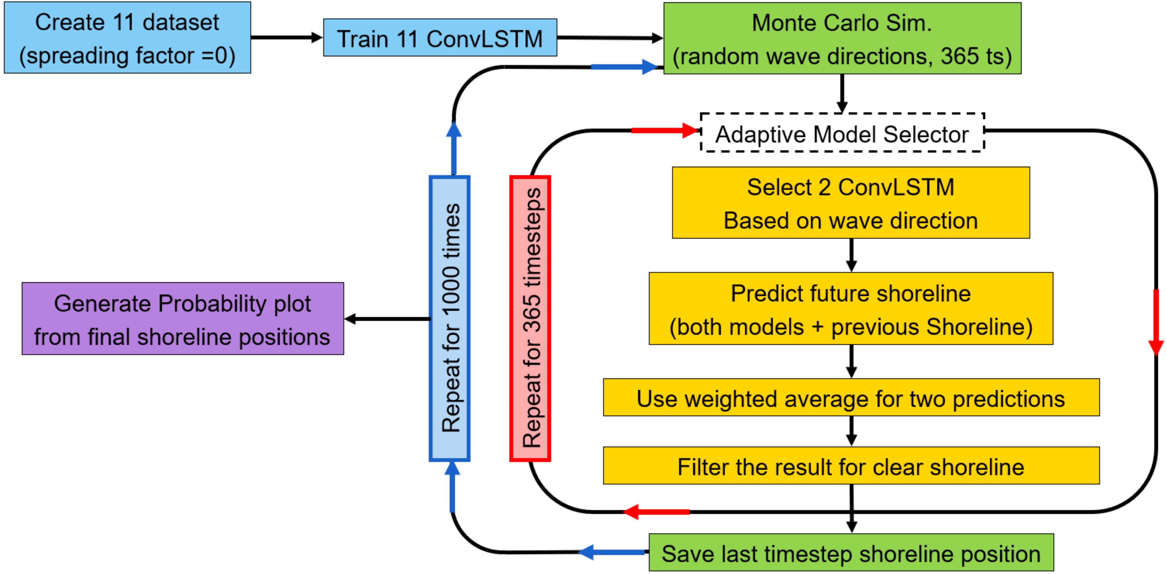
Figure 14. Flowchart of the proposed method combining pre-trained machine learning (adaptive model selector) and Monte Carlo simulation to generate the probability plot for shoreline positions.

As in the previous sections, the training and prediction of all ML models took place on Google Colaboratory servers, while the ShorelineS numerical model ran on a personal computer. The required time for completing the proposed method and obtaining 1000 final output from our numerical model and the final result are presented in Table 5 and Figure 15. As illustrated in Figure 13B and Figure 15, the probability plots are largely similar across most of the shoreline, except for specific areas like the lake on the lower right side. Major sections of the shoreline show consistent evolution probabilities. The slight differences in the lower right lake’s positioning may be due to low confidence in the model’s predictions. If predicted shoreline pixels are not well-aligned, those with lower probabilities may be removed during the filtering step. Additionally, the final results from the ShorelineS numerical model do not show high certainty, particularly around features like the head of the generated spit, even after multiple runs. In contrast, the Adaptive Model Selector method offers more coherent and better-correlated results for predicting shoreline positions in future timesteps, providing a clearer understanding of potential shoreline evolution.

Table 5

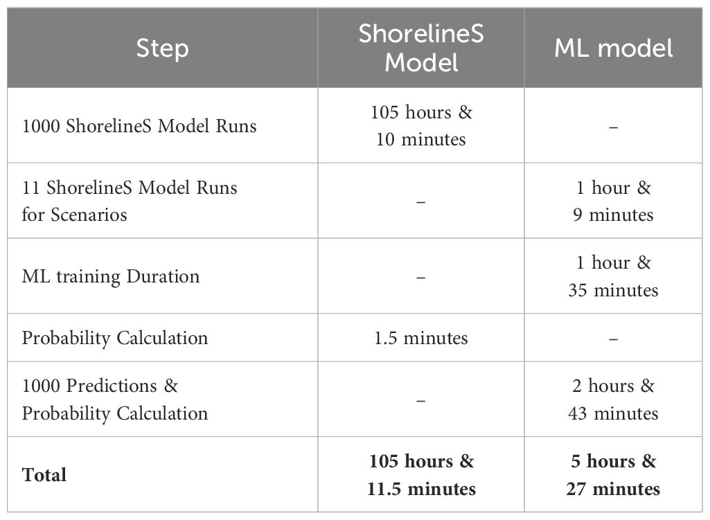
Table 5. Comparison of required time for analysing shoreline existence probability.

Figure 15

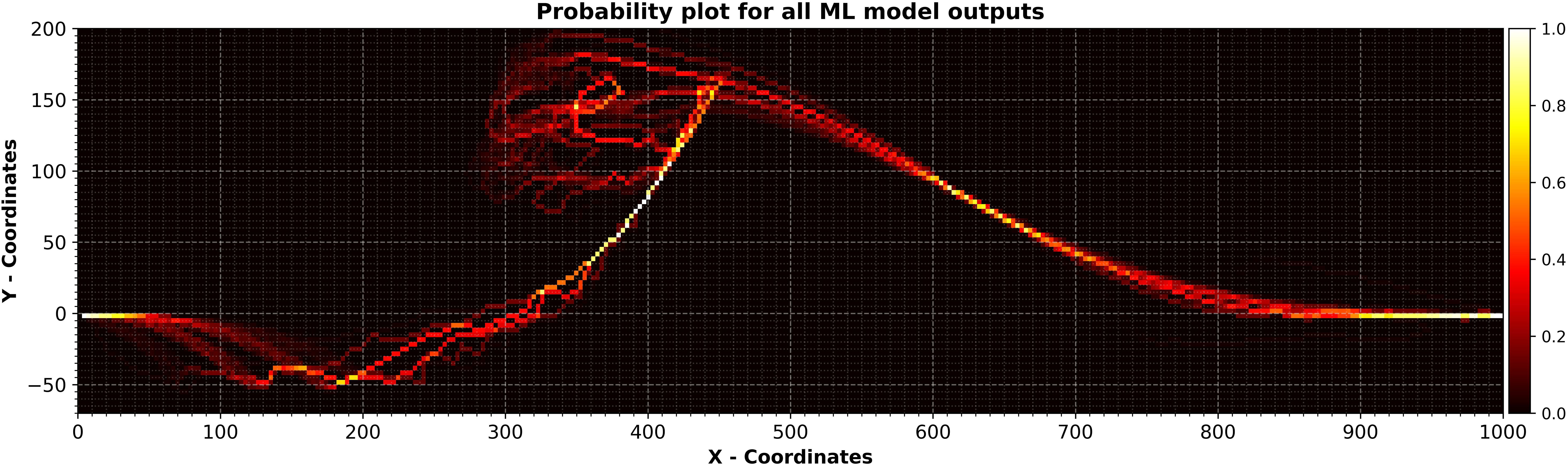
Figure 15. Probability plot for all shoreline positions at final timestep using adaptive model selector.

When comparing the runtime of the ShorelineS numerical model and the Adaptive Model Selector method, both run 1000 times to project future shoreline positions, the proposed method significantly reduces the required runtime by almost 95%.

5 Discussion

The results of this study demonstrate the efficacy of various ML models in predicting shoreline evolution with different input data structures. A key takeaway is the trade-off between computational efficiency and prediction accuracy when selecting an ML model. While simpler models like DNN can provide reliable predictions for relatively straightforward shoreline evolutions, more complex models such as ConvLSTM are necessary for capturing intricate shoreline behaviours, including island and lake formation.

A significant observation is the variation in prediction performance depending on the data structure used. Models trained with coordinate-based data generally performed well for cases without complex morphological changes. However, models trained on image or 2D gridded data exhibited superior predictive capabilities, particularly for scenarios involving shoreline features such as spits and islands. The ConvLSTM model trained on 2D gridded data emerged as the most robust, effectively balancing prediction accuracy and computational cost.

The DNN model demonstrated a reasonable ability to predict shoreline positions but struggled with cases involving significant morphological changes. Similarly, the LSTM model faced difficulties in learning from coordinate-based data, particularly when using a one-row representation. Even with a two-row representation, the LSTM model did not perform as well as expected, especially in capturing the evolution of complex features such as islands and spits. These results suggest that LSTM models may not be well-suited for this problem, as their sequential nature does not effectively capture the spatial dependencies necessary for accurate shoreline prediction.

CNN models, when trained on two-row data, provided more reliable predictions than LSTM models. However, the CNN model trained on image-based data significantly improved prediction quality by leveraging spatial relationships within shoreline evolution. One drawback of this approach is the sensitivity to input defects, which can introduce unintended artifacts in the predictions. Nonetheless, CNN models trained on image data proved to be a practical choice, particularly for cases where shoreline changes are more spatially complex.

ConvLSTM models further refined prediction accuracy, particularly when trained with 2D gridded data. Unlike the standard LSTM model, the ConvLSTM model effectively captured both temporal and spatial dependencies, making it the best-performing model in our study. The ability of the ConvLSTM model to handle structured data representations enabled it to provide highly accurate predictions, even for shoreline evolutions involving dynamic morphological changes.

Overfitting is a critical challenge in machine learning applications, as it hampers the model’s ability to generalize beyond the training data, leading to poor predictive performance on unseen shoreline conditions. In our study, we addressed this issue by implementing early stopping, a widely used regularization technique that monitors validation loss during training and halts the process when no further improvement is observed. This approach ensures that the model does not continue training beyond the point of optimal generalization, preventing it from memorizing noise and fluctuations in the training data.

While ML models offer a substantial reduction in computational time compared to traditional numerical models, certain challenges remain. One key issue is the sensitivity of ML models to anomalies in the dataset. As demonstrated in the CNN results, incorrect shoreline representations in the training data can lead to the model replicating these errors in predictions. Addressing this challenge requires careful preprocessing of training data and potential refinement of the ML pipeline to detect and correct such anomalies.

A novel contribution of this study is the application of ML for probabilistic shoreline evolution prediction. By using Monte Carlo simulations and a developed Adaptive Model Selector approach, we developed a probabilistic framework that estimates the likelihood of shoreline positions over time. The probability plots generated from the ConvLSTM model closely resemble those obtained from traditional numerical models, confirming the reliability of our ML-based probabilistic prediction method. Additionally, the ability of the Adaptive Model Selector to dynamically select appropriate pre-trained ML models based on wave direction improves prediction accuracy while maintaining computational efficiency.

The comparison of computational efficiency between ML models and traditional numerical models reveals significant advantages in using ML for shoreline evolution prediction. The ConvLSTM model with 2D gridded data achieved a near 95% reduction in runtime compared to the ShorelineS numerical model while maintaining comparable accuracy. This drastic reduction in computational time makes ML models a viable alternative for large-scale shoreline prediction studies where computational cost is a concern.

While more complex ML models generally improve prediction accuracy, they also come with increased computational requirements during the training phase. The results indicate that model selection should consider both prediction accuracy and computational constraints. For relatively simple shoreline changes, a DNN or CNN model offers a good balance between accuracy and efficiency. For complex cases involving the formation of shoreline features, ConvLSTM with 2D gridded data is the best choice.

6 Conclusions

This study evaluated machine learning models for shoreline evolution prediction, A main finding is that ConvLSTM trained on 2D gridded data provided the most accurate predictions, effectively capturing both general shoreline evolution and complex morphological features such as spits and lakes. While simpler models like DNN performed well for basic shoreline changes, more advanced architectures such as CNN and ConvLSTM demonstrated superior predictive capabilities for detailed and dynamic shoreline structures. However, this improvement came at the cost of increased training times due to the larger data volumes required for processing spatial and temporal dependencies.

The study also highlighted the trade-off between model complexity and computational cost. While deep learning models require longer training times than traditional numerical models, they can make rapid predictions once trained. Notably, models using matrix-based data, such as CNN and ConvLSTM, outperformed those relying on simpler two-row data representations.

To address uncertainties in shoreline position prediction, the Adaptive Model Selector was introduced. This method dynamically selects and combines predictions from pre-trained models, specifically leveraging the strengths of ConvLSTM trained on 2D gridded data, to improve accuracy across varying wave conditions. When integrated with Monte Carlo simulations, this approach accounted for wave-driven variability while significantly reducing computational time—achieving a 95% reduction compared to traditional methods.

In conclusion, this research demonstrates that machine learning, particularly ConvLSTM with 2D gridded data, provides a robust and efficient framework for shoreline evolution modeling. By leveraging ML-based approaches, coastal researchers and engineers can achieve higher accuracy in shoreline predictions while drastically reducing computational costs, making ML a promising alternative compare to traditional methods.

Data availability statement

The original contributions presented in the study are included in the article/Supplementary Material. Further inquiries can be directed to the corresponding author.

Author contributions

AS: Conceptualization, Data curation, Formal analysis, Investigation, Methodology, Project administration, Resources, Software, Supervision, Validation, Visualization, Writing – original draft, Writing – review & editing. AD: Conceptualization, Formal analysis, Methodology, Supervision, Writing – original draft, Writing – review & editing. DR: Conceptualization, Formal analysis, Methodology, Supervision, Writing – original draft, Writing – review & editing.

Funding

The author(s) declare that financial support was received for the research and/or publication of this article. The publication of this article as open access was financially supported by Delft University of Technology.

Acknowledgments

This article is derived from the first author’s MSc thesis titled “Machine Learning for Shoreline Change Prediction: Evaluation of Machine Learning Models for Predicting Shoreline Changes Using Synthetic Sequential Data”, completed at IHE Delft, referenced as Adeli Soleimandarabi (2023). The authors extend their gratitude to IHE Delft, TU Delft and Ghent University for their support and contributions during the research and writing process.

Conflict of interest

The authors declare that the research was conducted in the absence of any commercial or financial relationships that could be construed as a potential conflict of interest.

Generative AI statement

The author(s) declare that Generative AI was used in the creation of this manuscript. In the process of writing this article, the Grammarly AI tool was used to ensure clarity and grammatical precision in this work. Nevertheless, all research, insights, and conclusions presented here are a result of our comprehensive study and understanding of the topic.

Publisher’s note

All claims expressed in this article are solely those of the authors and do not necessarily represent those of their affiliated organizations, or those of the publisher, the editors and the reviewers. Any product that may be evaluated in this article, or claim that may be made by its manufacturer, is not guaranteed or endorsed by the publisher.

Supplementary material

The Supplementary Material for this article can be found online at: https://www.frontiersin.org/articles/10.3389/fmars.2025.1562504/full#supplementary-material

References

Adeli Soleimandarabi A. (2023). Machine learning for shoreline change prediction:Evaluation of machine learning models for predicting shoreline changes using synthetic sequential data [Master’s thesis] (Delft: IHE Delft Institute for Water Education). doi: 10.25831/81mk-zx14

Crossref Full Text | Google Scholar

Brady A. and Sutherland J. J. H. W. R. T. (2001). COSMOS modelling of COAST3D Egmond main experiment. 115. Howbery Park, Wallingford, OXON OX10 8BA: HR Wallingford Ltd.

Google Scholar

Brownlee J. (2018). “Deep learning for time series forecasting: predict the future with MLPs, CNNs and LSTMs in Python,” in Machine learning mastery. Australia: Jason Brownlee / Machine Learning Mastery.

Google Scholar

Choi H., Park M., Son G., Jeong J., Park J., Mo K., et al. (2020). Real-time significant wave height estimation from raw ocean images based on 2D and 3D deep neural networks. Ocean Eng. 201, 107129. doi: 10.1016/j.oceaneng.2020.107129

Crossref Full Text | Google Scholar

Dastgheib A. (2012). Long-term process-based morphological modeling of large tidal basins [DISSERTATION (DELFT: Delft University of Technology & UNESCO-IHE Institute for Water Education]).

Google Scholar

DHI Group (2020). “MIKE,” in In (Version 2020) (Hørsholm, Denmark: DHI Group). Available online at: https://www.mikepoweredbydhi.com/. (Accessed August 16, 2023).

Google Scholar

Goldstein E. B., Coco G., and Plant N. G. (2019). A review of machine learning applications to coastal sediment transport and morphodynamics. Earth-Science Rev. 194, 97–108. doi: 10.1016/j.earscirev.2019.04.022

Crossref Full Text | Google Scholar

Goodfellow I., Pouget-Abadie J., Mirza M., Xu B., Warde-Farley D., Ozair S., et al. (2014). Generative adversarial nets. 27. New York, NY, USA: Association for Computing Machinery.

Google Scholar

Google Co (2023). Google Colab GPU platforms. Available online at: https://cloud.google.com/compute/docs/gpusa100-gpus. (Accessed July 10, 2023).

Google Scholar

Grimes D. J., Cortale N., Baker K., and McNamara D. E. (2015). Nonlinear forecasting of intertidal shoreface evolution. Chaos 25, 103116. doi: 10.1063/1.4931801

PubMed Abstract | Crossref Full Text | Google Scholar

Gutierrez B. T., Plant N. G., and Thieler E. R. (2011). A Bayesian network to predict coastal vulnerability to sea level rise. J. Geophysical Research: Earth Surface 116. doi: 10.1029/2010JF001891

Crossref Full Text | Google Scholar

Hans H. (1989). Genesis: A generalized shoreline change numerical model. J. Coast. Res. 5, 1–27. Available at: http://www.jstor.org/stable/4297483. (Accessed July 3, 2023).

Google Scholar

Hashemi M. R., Ghadampour Z., and Neill S. P. (2010). Using an artificial neural network to model seasonal changes in beach profiles. Ocean Eng. 37, 1345–1356. doi: 10.1016/j.oceaneng.2010.07.004

Crossref Full Text | Google Scholar

He Q. and Silliman B. R. (2019). Climate change, human impacts, and coastal ecosystems in the anthropocene. Curr. Biol. , 29, R1021–R1035. doi: 10.1016/j.cub.2019.08.042

PubMed Abstract | Crossref Full Text | Google Scholar

Iglesias G., Diz-Lois G., and Pinto F. T. (2010). Artificial Intelligence and headland-bay beaches. Coast. Eng. 57, 176–183. doi: 10.1016/j.coastaleng.2009.10.004

Crossref Full Text | Google Scholar

James G., Witten D., Hastie T., and Tibshirani R. (2013). An introduction to statistical learning with applications in R. 1 ed (USA: Springer New York, NY). doi: 10.1007/978-1-4614-7138-7

Crossref Full Text | Google Scholar

Kamphuis J. W. (2010). Introduction to coastal engineering and management. 2nd ed (New Jersey: World Scientific). Available at: http://lib.ugent.be/catalog/rug01:002037065. (Accessed May 20, 2023).

Google Scholar

Kingston K. S., Ruessink B. G., van Enckevort I. M. J., and Davidson M. A. (2000). Artificial neural network correction of remotely sensed sandbar location. Mar. Geology 169, 137–160. doi: 10.1016/S0025-3227(00)00056-6

Crossref Full Text | Google Scholar

Kristensen S. E., Drønen N., Deigaard R., and Fredsoe J. (2016). Impact of groyne fields on the littoral drift: A hybrid morphological modelling study. Coast. Eng. 111, 13–22. doi: 10.1016/j.coastaleng.2016.01.009

Crossref Full Text | Google Scholar

Lu Y., Wang H., and Wei W. J. (2023). Machine learning for synthetic data generation: a review. arXiv, Ithaca, NY, USA. doi: 10.48550/arXiv.2302.04062

Crossref Full Text | Google Scholar

Mirtaheri S. L. and Shahbazian R. (2022). Machine learning theory to applications. 1st Edition ed (Taylor & Francis, Milton Park, Abingdon, Oxfordshire, UK: CRC Press).

Google Scholar

Mutagi S., Yadav A., and Hiremath C. G. (2022). Shoreline change model: A review. Sustainability trends and challenges in civil engineering Vol. 2022 (Singapore: Springer Nature Singapore Pte Ltd).

Google Scholar

Nicholls R. J. and Cazenave A. J. (2010). Sea-level rise its impact Coast. zones. 328, 1517–1520. Sea-Level Rise and Its Impact on Coastal Zones. Science 328, 1517–1520. doi: 10.1126/science.1185782

PubMed Abstract | Crossref Full Text | Google Scholar

Nicholls R. J., Wong P. P., Burkett V., Codignotto J., Hay J., McLean R., et al. (2007). Coastal systems and low-lying areas. Cambridge, UK: Cambridge University Press.

Google Scholar

Pedregosa F., Varoquaux G., Gramfort A., Michel V., Thirion B., Grisel O., et al. (2011). Scikit-learn: machine learning in python. J. Mach. Learn. Res. 12, 2825–2830. doi: 10.48550/arXiv.1201.0490

Crossref Full Text | Google Scholar

Pelnard-Considère R. (1956). Essai de théorie de l’évolution des formes de rivage en plages de sable et de galets (Société hydrotechnique de France). Lyon, France: University of Lyon, Persée.

Google Scholar

Plomaritis T. A., Costas S., and Ferreira Ó. (2018). Use of a Bayesian Network for coastal hazards, impact and disaster risk reduction assessment at a coastal barrier (Ria Formosa, Portugal). Coast. Eng. 134, 134–147. doi: 10.1016/j.coastaleng.2017.07.003

Crossref Full Text | Google Scholar

PMO, I. P. A. M. O (2013). “PMO dynamics,” in Iranian ports and maritime organization. PTehran, Iran: Ports and Maritime Organization (PMO). Available at: http://www.pmo.ir/. (Accessed June 18, 2023).

Google Scholar

Poelhekke L., Jäger W. S., van Dongeren A., Plomaritis T. A., McCall R., and Ferreira Ó. (2016). Predicting coastal hazards for sandy coasts with a Bayesian Network. Coast. Eng. 118, 21–34. doi: 10.1016/j.coastaleng.2016.08.011

Crossref Full Text | Google Scholar

Roelvink D., Huisman B. A. H., Elghandour A. H. H., Ghonim M. M., and Reyns J. (2020). Efficient modeling of complex sandy coastal evolution at monthly to century time scales. Front. Mar. Sci. 7. doi: 10.3389/fmars.2020.00535

Crossref Full Text | Google Scholar

Roelvink D., Reniers A., van Dongeren A., van Thiel de Vries J., McCall R., and Lescinski J. (2009). Modelling storm impacts on beaches, dunes and barrier islands. Coast. Eng. 56, 1133–1152. doi: 10.1016/j.coastaleng.2009.08.006

Crossref Full Text | Google Scholar

Roscher R., Bohn B., Duarte M. F., and Garcke J. (2020). Explainable machine learning for scientific insights and discoveries. IEEE Access 8, 42200–42216. doi: 10.1109/ACCESS.2020.2976199

Crossref Full Text | Google Scholar

Royal Haskoning D. H. V. (2020). CoastalFOAM. Available online at: https://coastalsolutions.ireport.royalhaskoningdhv.com/software-and-tools. (Accessed June 11, 2023).

Google Scholar

Solomatine D. P. (2023). Data-driven modeling: Machine learning, data mining and knoledge discovery [Lecture Note] (Westvest 7, 2611 AX Delft, The Netherlands: IHE Delft Institute for Water Education).

Google Scholar

Sutherland J., Peet A., and Soulsby R. J. C. (2004). Evaluating the performance of morphological models. Coastal Engineering 51, 917–939. doi: 10.1016/j.coastaleng.2004.07.015

Crossref Full Text | Google Scholar

Thambawita V. L., Salehi P., Sheshkal S. A., Hicks S., L.Hammer H., Parasa S., et al. (2021). SinGAN-Seg: Synthetic training data generation for medical image segmentation. 17. San Francisco, CA, USA: PLOS. doi: 10.1371/journal.pone.0267976

PubMed Abstract | Crossref Full Text | Google Scholar

Tonnon P. K., Huisman B. J. A., Stam G. N., and van Rijn L. C. (2018). Numerical modelling of erosion rates, life span and maintenance volumes of mega nourishments. Coast. Eng. 131, 51–69. doi: 10.1016/j.coastaleng.2017.10.001

Crossref Full Text | Google Scholar

Tsiakos C.-A. D. and Chalkias C. (2023). Use of machine learning and remote sensing techniques for shoreline monitoring: A review of recent literature. Appl. Sci. 13, 3268. Available at: https://www.mdpi.com/2076-3417/13/5/3268. (Accessed August 3, 2023).

Google Scholar

van Rijn L. C., Walstra D. J., Grasmeijer B., Sutherland J., Pan S., and Sierra J. J. C. E. (2003). The predictability of cross-shore bed evolution of sandy beaches at the time scale of storms and seasons using process-based profile models. Coastal Engineering 47, 295–327. doi: 10.1016/S0378-3839(02)00120-5

Crossref Full Text | Google Scholar

Warner T. T. (2010). Numerical weather and climate prediction (Cambridge, UK: Cambridge University Press). doi: 10.1017/CBO9780511763243

Crossref Full Text | Google Scholar

Zhou Z. H. (2012). Ensemble methods: foundations and algorithms (Boca Raton, Florida, USA: CRC press).

Google Scholar