Identification of mesoscale eddies based on improved YOLOv8 model: a case study in the South China Sea

Mesoscale eddies play a crucial role in energy transfer and material transport in the ocean. Accurate identification of mesoscale eddies is crucial for a deeper understanding of ocean internal dynamics, the development of marine resources, and the prediction of changes in the marine environment. This study utilizes Absolute Dynamic Topography (ADT) data provided by AVISO and the YOLOv8 algorithm model to investigate the identification of mesoscale eddies in the South China Sea (SCS). Due to its feature analysis and generalization capability, the YOLOv8 can successfully captures some mesoscale eddies undetected by the PET, thus track more mesoscale eddy trajectories. By enhancing the model’s input features and loss function, the YOLOv8 algorithm model has achieved high-precision identification of mesoscale eddies in the SCS with 93.9% Recall and 96.4% AP_0.5, radius and amplitude average errors kept under 5 km and 0.50 cm. The incorporation of sea surface current field has improved the characteristics of mesoscale eddies, resulting in a smaller bias. However, due to some obscured ADT information, there was a slight increase in the identification errors for eddies’ amplitude and radius. Under typhoon events, the model accurately captures the evolution of mesoscale eddy characteristics, demonstrating high reliability. The model’s high accuracy (90.5% Recall, 93.6% AP_0.5) for the transfer application in the Arabian Sea. Moreover, its accuracy in the transfer application to high-resolution products is also commendable. After only a few additional training rounds, the model achieves a high level of accuracy (90.0% Recall, 94.9% AP_0.5), highlighting its robust generalization capabilities and transfer potential. This study suggests that the improved YOLOv8 algorithm enables threshold-free identification of mesoscale eddies with strong prospects for generalization and transfer applications which are expected to provide richer and more accurate mesoscale eddy track data.

1 Introduction

Mesoscale eddies, categorized into cyclonic and anticyclonic types based on their rotational characteristics, are a critical component of the ocean’s dynamical system, exerting a significant influence on the global oceanic circulation and the material transport (Zhang et al., 2014). As quintessential manifestations of mesoscale physical processes in the ocean, mesoscale eddies are critical conduits for the cascading of energy between large-scale and small-scale water motions (Zhang and Qiu, 2018; Wang et al., 2022a). The typical spatial dimensions of these oceanic mesoscale eddies extend from tens to hundreds of kilometers, with temporal scales that span from several days to hundreds of days, and vertical extents that may plunge several kilometers deep, occasionally reaching the abyssal seafloor (McGillicuddy et al., 1998; Uchida et al., 2022). Mesoscale eddies can be distinguished from the broader oceanic currents by their rapid rotational velocities, pronounced convergence of eddy kinetic energy, and profound vertical impact (Gaube et al., 2019; Cao et al., 2022). They can typically induce substantial variations in sea level elevation, modulate marine biogeochemical processes, and exert a considerable influence on heat exchange, materials transportation, chlorophyll concentration, as well as seawater salinity and density (Levy, 2003; Chen et al., 2011; Dong et al., 2014, 2017; Xiu and Chai, 2020; van Westen and Dijkstra, 2021; Zhou et al., 2021), thereby impacting underwater acoustic communication pathways (Oka et al., 2009; Chaigneau et al., 2011; Guo et al., 2017; Liu et al., 2021; Zhou et al., 2021). Additionally, through their interactions with the atmosphere, these eddies can modulate the local sea surface wind field, cloud formation, and precipitation patterns (Frenger et al., 2013). Therefore, the precise delineation of mesoscale eddies holds substantial research significance across the disciplines of physical oceanography, ocean acoustics, and marine environmental studies.

Due to the lack of a unified and precise definition for mesoscale eddies, the most accurate method of identification to date is “expert visual identification”, which is a process that requires a significant expenditure of time and effort and is inevitably subject to certain human errors. Currently, the popular identification methods for mesoscale eddies can be categorized into four types: the physical parameter method (Okubo, 1970; Weiss, 1991; Jeong and Hussain, 1995; Liu et al., 2016), the geometric image method (Sadarjoen and Post, 2000; Nencioli et al., 2010), the hybrid method (Chelton et al., 2011; Mason et al., 2014; Pegliasco et al., 2022), and the artificial intelligence method. The physical parameter method, geometric algorithm, and hybrid algorithm all rely on preset thresholds, which introduces subjectivity in defining eddies. Establishing a universal detection threshold and rigid constraints is challenging, as they must accommodate the diverse conditions of the sea and the varying developmental stages of eddies. As a result, both the physical parameter method and the geometric image method struggle to adapt effectively to the dynamic changes in marine eddies due to environmental complexities.

In recent years, the rapid development of artificial intelligence has facilitated the extensive use of machine learning methods in marine science. Machine learning techniques are notably distinguished by their robust transfer learning capabilities, which hold promise for extending the universality of mesoscale eddy identification models and enabling effective identification across various maritime regions. Consequently, many researchers have adopted machine learning approaches for mesoscale eddy identification, leading to substantial advancements in the field. For instance, a machine learning method based on altimetry was proposed to detect and characterize mesoscale eddies using decision tree regression to estimate their lifecycles with a root mean square error of approximately five days (Ashkezari et al., 2016). The U-Net network architecture was also applied to identify oceanic mesoscale eddies, introducing EddyNet (Lguensat et al., 2018). Subsequent studies have improved upon U-Net, developing variants such as MU-Net (Saida and Ari, 2022), AttresU-Net (Zhang et al., 2022b), DPU-Net (Zhao et al., 2023) and PSA-EDUNet (Zhao et al., 2023). Other deep learning algorithms, such as PSPNet, DeepLabV3+, and BiSeNet, have been used for mesoscale eddy detection, outperforming traditional methods in identifying a greater number of eddies (Xu et al., 2021). Hybrid approaches combining traditional methods with deep learning, such as integrating AMEDA with Faster R-CNN or using dual attention mechanisms with ADT and SST data, have further enhanced recognition efficiency and accuracy (Li et al., 2022; Xie et al., 2024; Zhang et al., 2024). More recently, the 3D-U-Res-Net model has enabled efficient delineation of the three-dimensional structure of mesoscale eddies, identifying various vertical structures and cylindrical eddies in the Southern Ocean (Liu et al., 2024; Xu et al., 2024). Artificial intelligence methods have become a hot topic and research direction in the identification of mesoscale eddies.

The “You Only Look Once” (YOLO) series of deep learning models for multi-object detection has been widely adopted since 2016 (Redmon et al., 2016). The term “You Only Look Once” indicates that the model can produce results after a single examination of an image. In the ocean research, the YOLO algorithm has been applied to identify marine fish species (Jalal et al., 2020) and underwater debris (Xue et al., 2021) from deep-sea imagery, ships (Zhang and Zhang, 2019) and mesoscale eddies (Cao et al., 2022) from Synthetic Aperture Radar (SAR) imagery. For mesoscale eddy identification, the YOLO Feature (YOLOF) model was employed to detect mesoscale eddies in the SCS from 1993 to 2021 (Cao et al., 2022). This approach mitigated biases associated with subjective threshold settings in traditional methods, thereby enhancing the identification efficiency (Cao et al., 2022). Additionally, the YOLO (DAY) model was proposed for precise mesoscale eddy identification (Wang et al., 2022b). This model incorporates spatiotemporal attention mechanisms and applies data augmentation techniques to Sea Level Anomaly (SLA) images, focusing on the spatiotemporal distributions of eddies and maximizing identification efficiency. Furthermore, a YOLO-based detection model was constructed to automate the identification of submesoscale eddies in C-band satellite Synthetic Aperture Radar (SAR) imagery, and the spatial distribution disparities between submesoscale and mesoscale eddies were further explored (Zi et al., 2024). At present, research on mesoscale eddy recognition based on the YOLO framework primarily focuses on the detection task of mesoscale eddies, marking them with bounding boxes without identifying eddy contours. However, the YOLOv5 framework has integrated semantic segmentation capabilities into the model. Subsequent YOLO models have also been widely applied to semantic segmentation tasks across various scenarios, achieving excellent results (Kavitha and Palaniappan, 2023; Liu et al., 2023).

Therefore, this study aims to employ a semantic segmentation model under the YOLOv8 framework for the identification of mesoscale eddies. Based on its outstanding detection capability, the model will further discern the specific shapes of mesoscale eddies, benefit to study of the intensity, amplitude, and life cycle of mesoscale eddies.

2 Study area and dataset

The study area is the South China Sea and its adjacent waters (5~25°N, 105~125°E; Figure 1). The SCS is the largest marginal sea of the East Asian continent, with a complex topography and hydrodynamics, which are conducive to the generation of various types of mesoscale eddies.

Figure 1

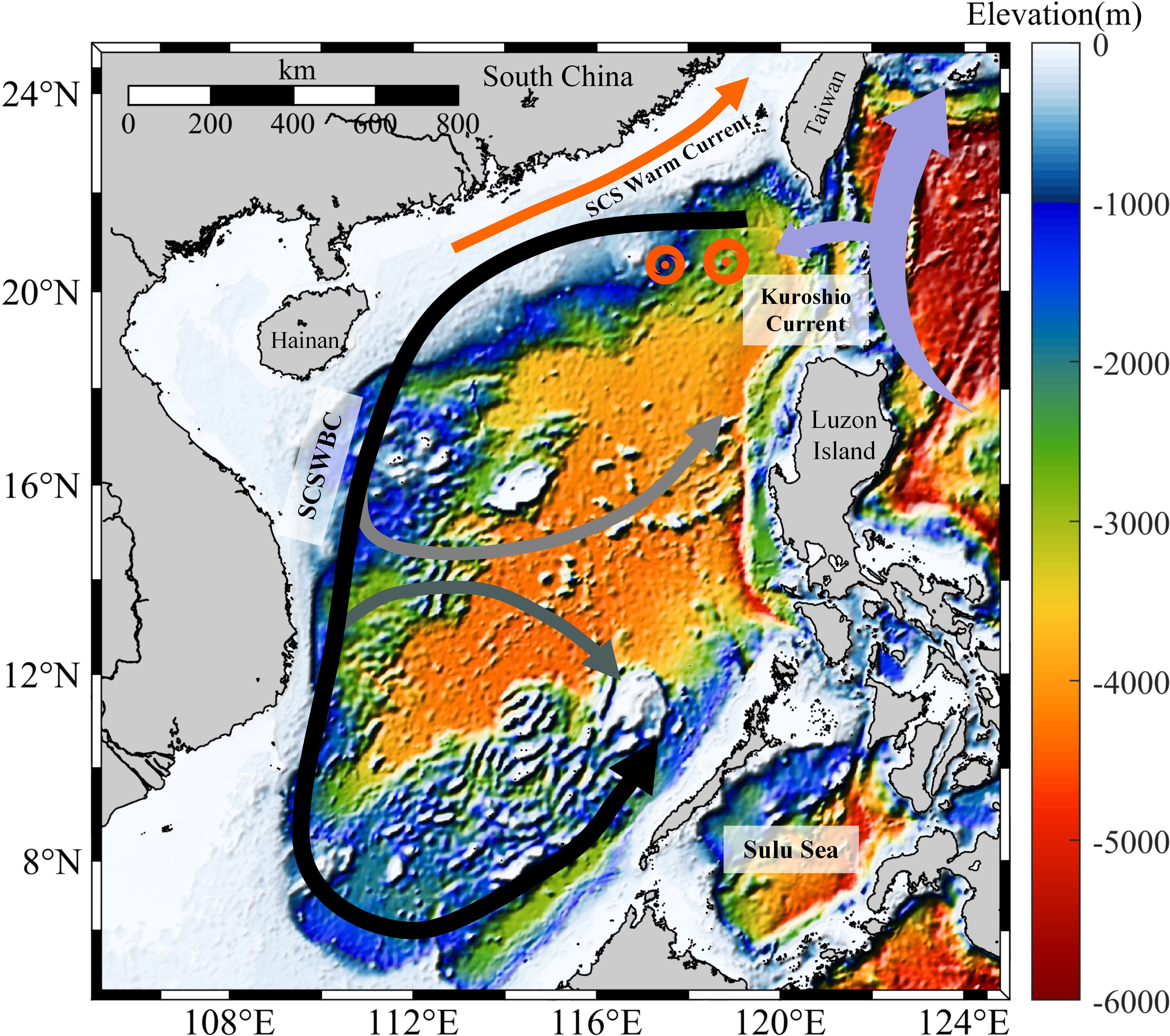
Figure 1. Study area: South China Sea (SCS). The bottom map illustrates the topographic structure of the SCS. The primary circulation structures in the SCS include the South China Sea West Boundary Current (SCSWBC), which exhibits east-west flow in the central region of the SCS, and the SCS Warm Current located in the northern part of the SCS. Additionally, the Kuroshio Current intermittently intrudes into and generates warm eddies in the Luzon Strait.

Mesoscale eddies in the SCS are primarily influenced by three factors: terrain undulations, the intrusion of the Kuroshio Current, and the impact of monsoons (Wu and Chiang, 2007; Wang et al., 2012a; Yang et al., 2022). The multi-scale circulation in the SCS is primarily regulated by monsoons and the exchange process with the Pacific Ocean. The Kuroshio Current, as a strong western boundary current of the North Pacific, plays a crucial role in the water exchange process between the SCS and the North Pacific (Chu et al., 1999; Yang et al., 2019). When the Kuroshio passes through the Luzon Strait, it forms a bend, intermittently invading the SCS and shedding anticyclonic eddy flows (Yang et al., 2019). The intensity of the Kuroshio exhibits periodic variations, affecting the multi-scale circulation and mesoscale processes in the SCS differently across years and seasons (Nan et al., 2015). Notably, the Kuroshio’s intrusion and eddy shedding peak in winter, likely due to the Ekman drift induced by the winter northeast monsoon, which pushes the Kuroshio into the SCS and triggers westward transport and eddy formation (Jia and Chassignet, 2011). The interaction of dynamic factors such as topographical variations, monsoon effects, the Kuroshio Current, and multi-scale circulation leads to baroclinic instability, causing the SCS to exhibit a high frequency of mesoscale eddies, a broad distribution of eddies, and significant eddy kinetic energy compared to the open ocean. At the same time, various eddy phenomena such as single eddies, eddy dipoles, and eddy groups all occur in the SCS. Therefore, the complex driving mechanisms and diverse types of eddies make the SCS a typical area for conducting mesoscale eddy research.

This study utilizes the Ssalto/Duacs altimetry products released by the Archiving Validation and Interpretation of Satellite Oceanographic (AVISO+), which is a multi-mission merged altimeter data product. These products are processed by the Data Unification and Altimeter Combination System (DUACS) multi-mission altimeter data processing system. The system handles data from various altimeter missions, including Jason-3, Sentinel-3A, HY-2A, Saral/AltiKa, Cryosat-2, Jason-2, Jason-1, T/P, EN-VISAT, GFO, and ERS1/2. Currently, the data set is managed and distributed by the Copernicus Marine Environment Monitoring Service (CMEMS). The marine remote sensing data product employed in this study is the Map of Absolute dynamic topography (MADT). This product has a spatial resolution of 0.25° by 0.25° and a temporal resolution of 1 day. The ADT is calculated using Equation 1.

$\begin{array}{ll}\begin{array}{c}\mathit{A}\mathit{D}\mathit{T}=\mathit{S}\mathit{L}\mathit{A}+\mathit{M}\mathit{D}\mathit{T} \end{array}& (1)\end{array}$

where, ADT is the absolute dynamic topography, the sea level anomaly (SLA) is defined as the height difference between the actual sea level and the mean sea level. The current version of the mean sea surface height is derived from averaging the sea surface height values over a 20-year period from 1993 to 2012. Additionally, SLA is obtained by integrating measurements from different altimeter missions and applying optimal interpolation. Mean dynamic topography (MDT) refers to the average of the dynamic topography. Some of the eddies in the SCS are formed in coastal and variable depth areas, which are the result of wind-topography effects and current reflections. These dynamic processes leave imprints on the MDT (Pegliasco et al., 2022). Therefore, this ADT dataset facilitates a more comprehensive identification of mesoscale eddies in the South China Sea.

Furthermore, the absolute dynamic geostrophic velocity can be calculated from the ADT data using the Equations 2 and 3:

$\begin{array}{ll}\begin{array}{c}\mathit{u}=-\frac{\mathit{g}}{\mathit{f}}\frac{\mathbf{\partial }\mathit{A}\mathit{D}\mathit{T}}{\mathbf{\partial }\mathit{y}},\mathit{v}=\frac{\mathit{g}}{\mathit{f}}\frac{\mathbf{\partial }\mathit{A}\mathit{D}\mathit{T}}{\mathbf{\partial }\mathit{x}}\end{array}& (2)\end{array}$

$\begin{array}{ll}\begin{array}{c}\mathit{s}\mathit{p}\mathit{e}\mathit{e}\mathit{d}=\sqrt{({\mathit{u}}^{\mathbf{2}}+{\mathit{v}}^{\mathbf{2}})}\end{array}& (3)\end{array}$

where, u and v represent the zonal (west-east) and meridional (south-north) components of the absolute dynamic geostrophic velocity, respectively. f denotes the Coriolis parameter, g is the acceleration due to gravity, and speed refers to the magnitude of the absolute dynamic geostrophic velocity.

3 Deep learning model

3.1 YOLOv8 algorithm model

YOLOv8 is an open-source algorithmic model released by Ultralytics in January 2023, supporting three branch tasks: image classification, object detection, and instance segmentation (Jocher et al., 2023). The framework of the YOLOv8 algorithm is depicted in Figure 2 and consists of three parts: the backbone, the neck, and the head, totaling 22 layers. For the first time, YOLOv8 introduces the Faster Implementation of CSP Bottleneck with 2 convolutions (C2f) module. The C2f module adds more cross-layer connections, providing the model with richer gradient flow information. Within the backbone, the first and second layers use two consecutive convolutional networks with a 3×3 kernel, followed by downsampling, resulting in larger-scale feature maps. The Spatial Pyramid Pooling-Fast (SPPF) module employs a serial and parallel form of maxpool2d, achieving better feature fusion. The neck utilizes the Path Aggregation Feature Pyramid Network (PAFPN) structure, enhancing the bottom-up information transfer path through a combination of upsampling and downsampling processes. The neck also uses low-level features for precise localization to improve information transfer efficiency, with a fully connected layer fusion structure that provides a richer source of information for mask prediction.

Figure 2

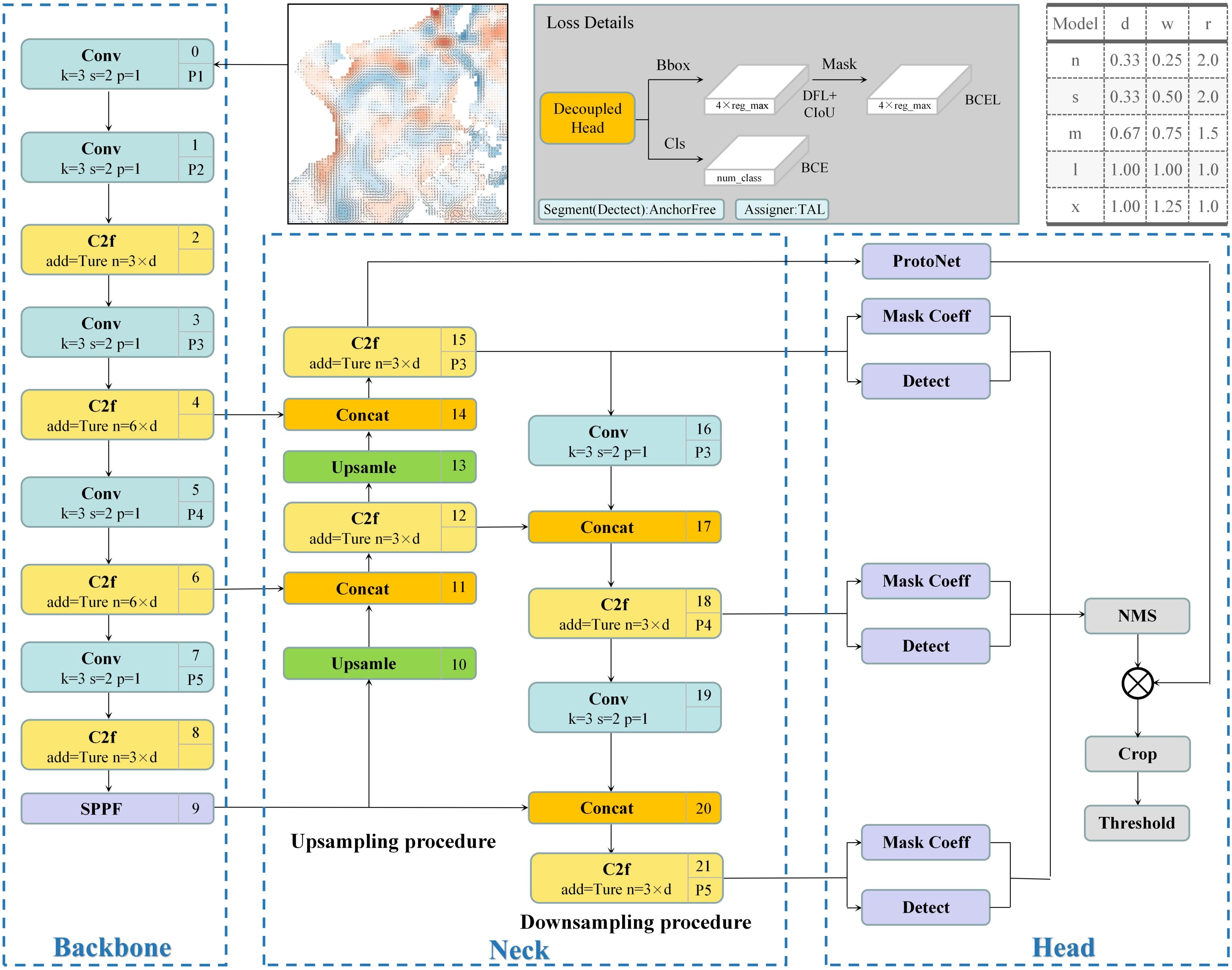
Figure 2. YOLOv8 algorithm framework diagram (d, w and r are model depth, width and ratio, respectively); In C2f module, h is the height, w is the width, and c is the number of channels. In the convolution module, k is the convolution kernel size, s is the operation step size, and p is the filling size of 0 value. After Jocher et al (Jocher et al., 2023).

In the segmentation task of the YOLOv8 model, a segmentation branch (Mask) runs parallel to the existing detection branch (Detect) in the prediction head. The head has evolved from a coupled head in the previous version to a more advanced decoupled head, separating the classification and regression tasks. This allows each task to be completed more independently and efficiently. Finally, this branch outputs the category of the eddy, as well as its bounding box information and k mask coefficients (ranging from -1 to 1) for each target eddy.

In the Protonet of the segmentation module, the input is the highest resolution image from the FPN. This facilitates enhanced preservation of spatial detail information within the ADT, while also offering valuable semantic insights. Since there are k different input images, the segmentation branch will output k prototype mask images (Prototype) for all input images. After completing the detection and segmentation branches, Non-Maximum Suppression (NMS) is utilized to retain optimal values in the prediction head results, reducing spatial overlap in recognition results. Finally, for each detected mesoscale eddy, we apply a linear combination of k mask coefficients to k prototype mask images. Then, the results are summed and passed through a sigmoid nonlinear function to obtain final mesoscale eddy instance segmentation results.

The regression branch loss function employs Complete Intersection over Union (CIoU) and Distribution Focal Loss (DFL), while the classification branch loss function utilizes Binary Cross-Entropy (BCE). In the instance segmentation task, the regression branch loss function also leverages BCE to calculate the loss between the predicted mask and the target mask. The overall model loss is the weighted sum of the regression and classification branch losses. YOLOv8 offers five models of varying scales, designated as n (nano), s (small), m (medium), l (large), and x (extra large). Each model features a distinct number of channels in its backbone network, and they do not strictly adhere to the same scaling factors. This design is beneficial for meeting the task requirements across different scenarios.

3.2 Loss function

The detection box loss (Bbox loss), calculated within the regression branch, is composed of two parts: CIoU and DFL. The expression for CIoU is shown in Equation 4 (Zheng et al., 2020):

$\begin{array}{ll}\begin{array}{c}{L}_{CIoU}=1-IoU+\frac{{\rho }^2(b,b^{gt})}{c^2}+\alpha v\end{array}& (4)\end{array}$

where, IoU represents the Intersection over Union between the predicted box and the ground truth box. b and $b^{gt}$ denote the predicted box and the ground truth box, respectively. ρ is the distance between the centers of the predicted box and the ground truth box, c is the diagonal distance between the two boxes, and α is the weight coefficient. v is a parameter that measures the consistency of the aspect ratio between the predicted and ground truth boxes. The specific expressions for v and α are shown in Equations 5 and 6:

$\begin{array}{ll}\begin{array}{c}v=\frac{4}{{\pi }^2}{(arctan\frac{w^{gt}}{h^{gt}}-arctan\frac{w}{h})}^2\end{array}& (5)\end{array}$

$\begin{array}{ll}\begin{array}{c}\alpha =\frac{v}{(1-IoU)+v}\end{array}& (6)\end{array}$

where, $w^{gt}$ and $h^{gt}$ represent the width and height of the detection box, respectively, while w and h denote the width and height of the ground truth box.

During the model training phase, multiple detection boxes are generated, and the probability is uniform across all points within the box. The DFL can assign a higher probability to points that are closer to the target point, enabling the network to quickly focus on the area surrounding the target point, thereby enhancing the effectiveness of network learning. The expression for DFL is shown in Equation 7 (Li et al., 2020):

$\begin{array}{ll}\begin{array}{c}DFL(S_i,S_{i+1})=-((y_{i+1}-y)\log (S_i)+(y-y_i)\log (S_{i+1}))\end{array}& (7)\end{array}$

where, $S_i$ represents the probability of each point, and $y_i$ denotes the location of the target point.

The Mask loss is calculated in the regression branch following the detection box loss, and is derived using Binary Cross Entropy with Logits. This function employs the log-sum-exp technique to combine the Sigmoid layer and the BCE in a single computation. The specific form of log-sum-exp is shown in Equation 8:

$\begin{array}{ll}\begin{array}{c}log-sum-\exp (x_1,x_2,\dots ,x_n)=\log ({\sum }_{i=1}^n{e}^{x_i-c})\end{array}& (8)\end{array}$

The classification loss in the classification branch is directly calculated using BCE. The expression for BCE is shown in Equations 9 and 10:

$\begin{array}{ll}\begin{array}{c}l(x,y)=L_{BCE}=\{l_1,l_2,\dots ,l_n\}\end{array}& (9)\end{array}$

$\begin{array}{ll}\begin{array}{c}{l}_n=-w_n[y_n·log(x_n)+(1-y_n)·log(1-x_n)]\end{array}& (10)\end{array}$

where, $L_{BCE}$ represents the Binary Cross-Entropy loss, x is the predicted value with a range of (0,1), y is the label value which is either 0 or 1, and $w_n$ is the weight coefficient.

3.3 Data set production

A total of 3653 daily ADT data spanning a decade from 2011 to 2020 were used as the training set, and the 365 daily ADT data from 2021 served as the validation set. The mesoscale eddies identified by the PET method is used as the Label in deep learning models. The PET method identifies closed contour lines of the ADT within a range of -100 cm to 100 cm with a search interval of 0.2 cm based on the input ADT data field. After the closed contours are identified, they must meet the following criteria to be classified as mesoscale eddies (Pegliasco et al., 2022): (1) Shape detection: The difference between the area of the closed contour and the area of its fitted circle, relative to the fitted circle area, is less than or equal to 55%. (2) Area detection: The closed contour must contain ADT data points ranging from 4 to 1000. (3) Consistency detection: The closed contour must only include data points with ADT values higher (lower) than the current ADT interval value for anticyclonic (cyclonic) eddies. (4) Single extremum detection: An anticyclonic (cyclonic) eddy should have no more than one maximum (minimum) ADT value within its interior. (5) Amplitude detection: The amplitude of the closed contour must be within the range of 1-150 cm.

Prior to being input into the YOLOv8 model for training, the ADT data underwent high-pass filtering with a 700 km radius in order to eliminate the influence of large-scale motions and highlight the image features of mesoscale processes. The input image size is 648×648 pixels, which is close to the maximum image resolution supported by the YOLOv8 model. This enhances the model’s ability to extract features across the entire marine area and mitigates the risk of feature loss resulting from image segmentation and compression.

3.4 Model evaluation index

The images of ocean mesoscale eddies detected by the YOLOv8 model are compared with the labeled images of the ocean mesoscale eddy dataset. If the network’s segmentation result matches the standard segmentation result, it is classified as a True Positive (TP); otherwise, it is considered a False Positive (FP). For pixels that are not part of mesoscale eddies, if the network’s segmentation result is correct, it is a True Negative (TN); otherwise, it is it is a False Negative (FN).

This experiment utilized three common metrics at the pixel level from the field of image segmentation to assess the results, including Precision, Recall, the Dice coefficient (F1), and Average Precision (AP). These metrics were employed to evaluate the outcomes accurately and effectively, with accuracy being regarded as the mesoscale eddy identification rate.

Precision measures the accuracy of the positive predictions made by the model, as shown in Equation 11.

$\begin{array}{ll}\begin{array}{c}Precision=\frac{TP}{TP+FP}\end{array}& (11)\end{array}$

Recall quantifies the model’s ability to detect all positive instances, as shown in Equation 12.

$\begin{array}{ll}\begin{array}{c}Recall=\frac{TP}{TP+FN}\end{array}& (12)\end{array}$

The precision rate indicates the proportion of mesoscale eddies that are correctly predicted, such that when the Precision is at 100%, there are no FP. The recall rate represents the proportion of eddies that the model correctly detects out of all labeled mesoscale eddies, meaning that at 100% recall, there are no FN. However, since Precision and Recall are inversely related, neither Precision nor Recall alone can fully encapsulate the model’s identification capabilities. Thus, this study also utilizes more comprehensive evaluation metrics: the F1, AP_0.5 and AP_0.5-0.95.

The F1 score is the harmonic mean of the model’s precision and recall, providing a more comprehensive assessment of the classification model’s performance, as shown in Equation 13.

$\begin{array}{ll}\begin{array}{c}F1=\frac{2*Precision*Recall}{Precision+Recall}\end{array}& (13)\end{array}$

AP_0.5 refers to the area under the Precision-Recall curve of the model, with a value closer to 1 indicating superior model performance, as shown in Equation 14. The subscript 0.5 indicates that a predicted target is considered a true positive (i.e., a mesoscale eddy) only if the Intersection over Union (IoU), which measures the overlap between the predicted target and the ground truth, is at least 0.5. When the IoU threshold is set to 0.5, varying the confidence threshold generates multiple pairs of Recall and Precision, thus forming the Precision-Recall curve.

$\begin{array}{ll}\begin{array}{c}A{P}_{0.5}={\int }_0^{1}Precision(Recall)dRecall\end{array}& (14)\end{array}$

AP_0.5-0.95 is calculated by determining the AP_IoU across multiple IoU thresholds ranging from 0.5 to 0.95 (with a step size of 0.05) between predicted and true targets. The average of these AP_IoU is then taken. This metric reflects the model’s overall recognition capability under different evaluation criteria.

mAP (mean Average Precision) is the average of the AP_0.5-0.95 for cyclonic and anticyclonic mesoscale eddies.

3.5 Experimental environment and parameter setting

This study employed a deep learning experimental environment within the PyCharm framework, with the following specific hardware, software, and system configurations: CPU: Intel Xeon Processor (Skylake, IBRS) × 2, GPU: NVIDIA Tesla T4 × 2, Python: 3.8, CUDA: 11.3, operating system: Ubuntu 16 LTS, and memory: 32.00 GB. For the YOLOv8 model parameter settings, the training batch size was set to 16, with a total of 200 training epochs. The initial learning rate was 0.01, which was reduced to a final learning rate of 0.0001. The optimizer used was SGD, with a dropout regularization rate of 0.2. The mask downsampling rate was set to 4.

4 Experiment and result

4.1 Sensitivity of identification accuracy to input field and loss function

In the computation of the Bbox loss, although the CIoU loss takes into account the overlapping area, the distance between centers, and the aspect ratio similarity, the aspect ratio consistency parameter v is not well-defined. The aspect ratio consistency parameter v may lead to unreasonable optimization and to some extent slow down the convergence speed of the YOLOv8 model. Given that mesoscale eddies are generally quasi-circular, the width and height of their bounding boxes can more directly reflect their shape characteristics. Therefore, this study proposes using Focal EIoU instead of CIoU for calculating the Bbox loss. EIoU, which is based on CIoU, calculates the width loss and height loss of the bounding box separately. This approach addresses a limitation in CIoU where focusing solely on aspect ratio loss prevents simultaneous adjustments in width and height losses. Consequently, it aligns more closely with the morphological characteristics of mesoscale eddies. Additionally, the introduction of Focal Loss optimizes the imbalance of samples in regression tasks and mitigates the negative impact of low-quality samples on the gradient. This approach focuses on high-quality bounding boxes, enhancing the model’s training accuracy and convergence rate. The expression for Focal EIoU is shown in Equations 15 and 16 (Zhang et al., 2022a):

$\begin{array}{ll}\begin{array}{c}{L}_{EIoU}=L_{IoU}+L_{dis}+L_{asp}=1-IoU+\frac{{\rho }^2(b,b^{gt})}{c^2}+\frac{{\rho }^2(w,w^{gt})}{C_w^2}+\frac{{\rho }^2(h,h^{gt})}{C_h^2}\end{array}& (15)\end{array}$

$\begin{array}{ll}\begin{array}{c}{L}_{FocalEIoU}=Io{U}^{\gamma }{L}_{EIoU}\end{array}& (16)\end{array}$

To highlight the sensitivity of identification accuracy to input field and loss function, the experiment utilizes the most lightweight version of the YOLOv8 model, hereafter referred to as YOLOv8, to conduct a sensitivity analysis on two types of loss functions (i.e., CloU and Focal EIoU) and input fields (i.e., ADT and uv). The experiment designs are presented in Table 1 and Table 2.

Table 1

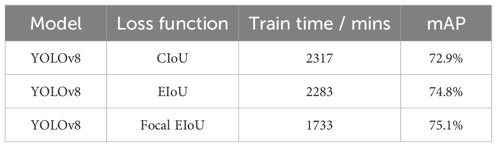
Table 1. Model training time and mAP under different loss functions.

Table 2

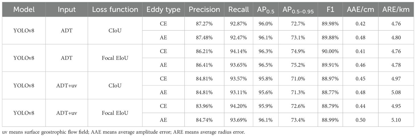
Table 2. Results of mesoscale eddy identification under different loss functions and input data.

Table 1 reveals that the YOLOv8 model, utilizing the EIoU loss function, exhibits a marginal decrease in training duration and a 1.9% increase in mAP relative to its predecessor. Subsequent integration of Focal loss into the model leads to a more pronounced reduction in training time by 25.2% and a 2.2% boost in mAP. These enhancements in loss functions are shown to markedly improve the efficiency of model training and the precision of recognition. Table 2 demonstrates that the YOLOv8 model attains the optimal recall rate, when using the Focal EIoU loss function with both ADT and uv data inputs. With the Focal EIoU loss function and ADT as the sole input, the model achieves more accurate mesoscale eddy identification, evidenced by the minimal average errors in amplitude and radius, along with the highest AP_0.5, AP_0.5-0.95 and F1 scores. Detailly, transitioning from the CIoU loss function to the Focal EIoU loss function improves the YOLOv8 model’s identification rate and precision for mesoscale eddies, as evaluated by the F1, AP_0.5 and AP_0.5-0.95 metrics. However, under the same confidence, the model’s Precision and Recall exhibit fluctuations, yet remain consistently high. The inclusion of uv data enriches the eddy characteristics with the dynamics of geostrophic flow fields, facilitating the model’s ability to discern features beyond ADT variations and leading to the detection of an increased number of mesoscale eddies. However, the introduction of uv data, which can only represent a single physical attribute per pixel (either uv or ADT), may overshadow certain information within the ADT data, resulting in greater shape errors (amplitude and radius) in the identified mesoscale eddies.

Figure 3 compares the performance of the YOLOv8 model with other AI models in the identification of mesoscale eddies. It is evident that the YOLOv8 model outperforms other models across various evaluation metrics. The model achieves higher scores in the more objective and balanced metrics of F1 and mAP, indicating greater stability and reliability in practical applications.

Figure 3

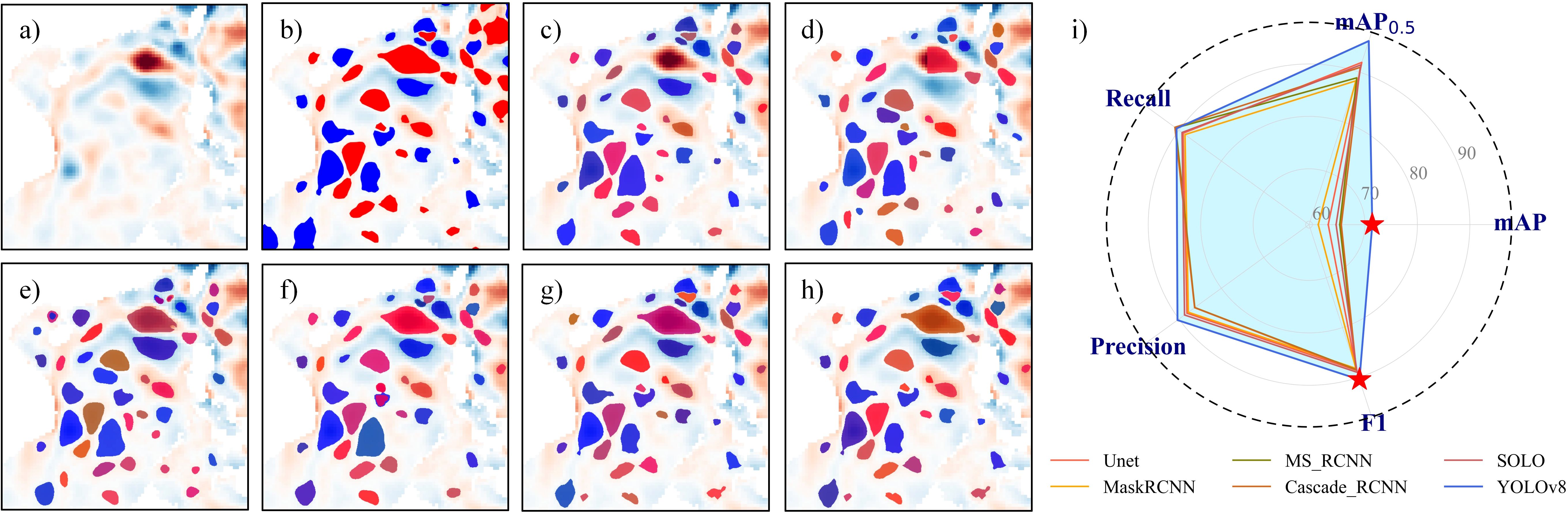
Figure 3. (a) Filtered ADT at 700 km. (b) Identification using PET method. (c–h) Identification results for Unet, MaskRCNN, MS_RCNN, Cascade_RCNN, SOLO, and YOLOv8. Warm colors and cool colors respectively represent anticyclonic and cyclonic eddies. (i) Comparative accuracy metrics, with F1 and mAP as key indicators; asterisk denotes YOLOv8 results.

Figure 4 further reveals that the YOLOv8 model can detect the majority of eddies identified by the original annotation methods and also uncover some previously overlooked mesoscale eddies based on the training data. Furthermore, the simultaneous input of uv and ADT data, under identical training conditions, enhances the model’s ability to identify mesoscale eddies, enabling it to recognize a broader spectrum of smaller-scale mesoscale eddies.

Figure 4

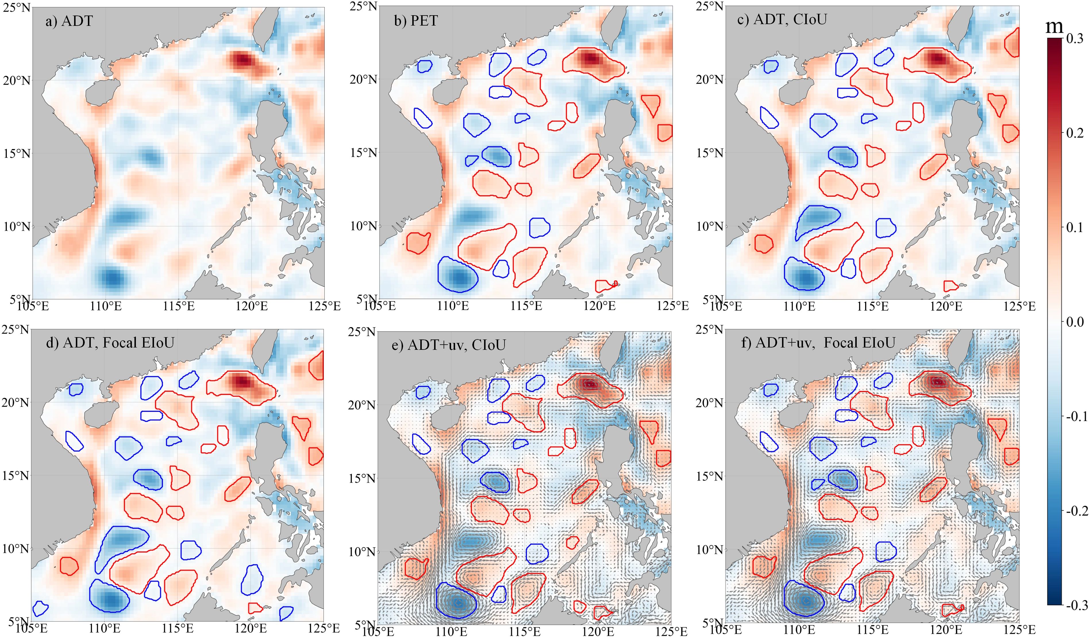
Figure 4. Comparisons of mesoscale eddies identification in the SCS on January 13, 2021. (a) the filtered ADT at 700km. (b–f) the results using the PET method and four YOLOv8 models. Blue represents cyclonic eddies, red represents anticyclonic eddies, and arrows represent sea surface geostrophic flow.

4.2 Statistical characteristics of SCS mesoscale eddies

The YOLOv8 model achieves high precision in mesoscale eddy identification, with an average precision higher than 95% and an F1 score higher than 88%, under four different input conditions and loss functions (Table 2). According to the evaluation using the AP_0.5 and the F1 score, the YOLOv8 model with ADT as the input field and the Focal EIoU as the loss function was selected for the statistical analysis of eddy characteristics in the SCS for the year 2021 test set.

As illustrated in Figure 5a, the daily count of eddy identification by the YOLOv8 model is comparable to that of the PET method, indicating a certain level of reliability in the YOLOv8 model’s identification outcomes. The quantity of mesoscale eddies in the SCS exhibits significant seasonal variations, with an increase observed in the spring of 2021, peaking in May, followed by a gradual decline during summer and autumn, and a slight resurgence in winter. The seasonal statistical analysis of the number and eddy kinetic energy (EKE) in the SCS shows that in spring, the mesoscale eddies in the SCS are smaller but larger in number, and the average EKE in the SCS is lower. In autumn, the mesoscale eddies are larger in scale, fewer in number, and the average EKE of the SCS remained low (Wang et al., 2012b; Xia and Shen, 2015). The variation characteristics of the number of eddies in 2021 are consistent with these findings. Figures 5b, c reveal that the YOLOv8 model identifies a greater number of eddies compared to the PET algorithm, particularly within the radius range of 25-50 km and amplitude range of 5~10 cm, where it detects a significant increase in eddy counts. This enhancement can be ascribed to two primary factors: firstly, the higher frequency of eddies within this radius and amplitude range in the SCS, providing a larger base for identification; secondly, the YOLOv8 model’s ability to identification eddies without being constrained by fixed physical thresholds, thereby capturing eddies that were previously overlooked. In statistical analyses for other radii or amplitude ranges, the YOLOv8 model identifies more eddies, except for those with amplitudes in the 25~30 cm interval. However, given the small proportion of eddies with radii exceeding 75 km or amplitudes above 15 cm within the total eddy population of the SCS, the additional detections by the YOLOv8 model in these categories are relatively constrained.

Figure 5

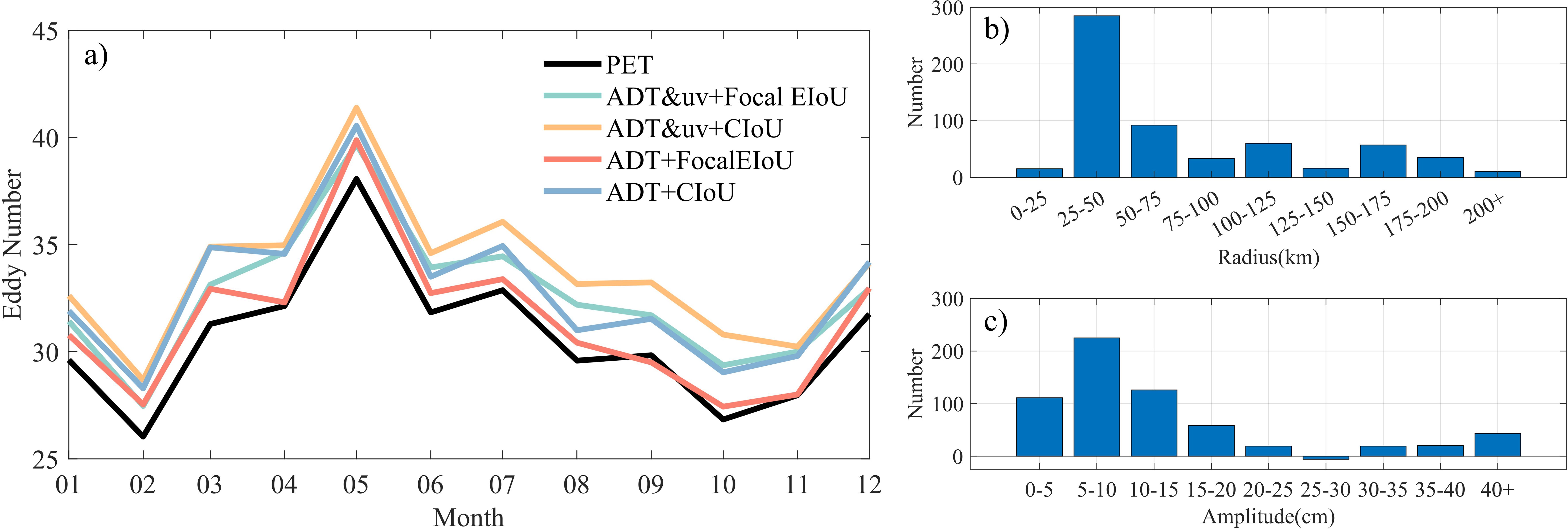
Figure 5. (a) Daily variations in the number of mesoscale eddies in the SCS in 2021. (b, c) the additional eddies identifications by the YOLOv8 model over the PET method for different radii and amplitudes in 2021.

The average radius of cyclonic mesoscale eddies in the SCS for 2021 is 68 km, with an average amplitude of 4.95 cm; for anticyclonic eddies, the average radius is 73 km, with an average amplitude of 5.84 cm (Figures 6a, b). There is a higher frequency of mesoscale eddies with a radius of 30~50 km. Within this range, cyclonic eddies outnumber anticyclonic ones. In terms of amplitude frequency distribution, anticyclonic and cyclonic eddies are largely consistent but there is a slight predominance of cyclonic eddies over anticyclonic ones in smaller amplitudes. As illustrated in Figure 6e, the baroclinic Rossby deformation radius is generally less than 50 km in most maritime regions located north of 10°N. Furthermore, over 80% of the identified eddies exceed their local baroclinic Rossby deformation radius, suggesting that these eddies are classified as mesoscale phenomena. Due to the influence of the baroclinic Rossby deformation radius and the positive correlation (r = 0.71) between eddy radius and amplitude (Figure 6f), mesoscale eddies in the SCS can attain radii up to 100 km and amplitudes surpassing 20 cm remain relatively infrequent.

Figure 6

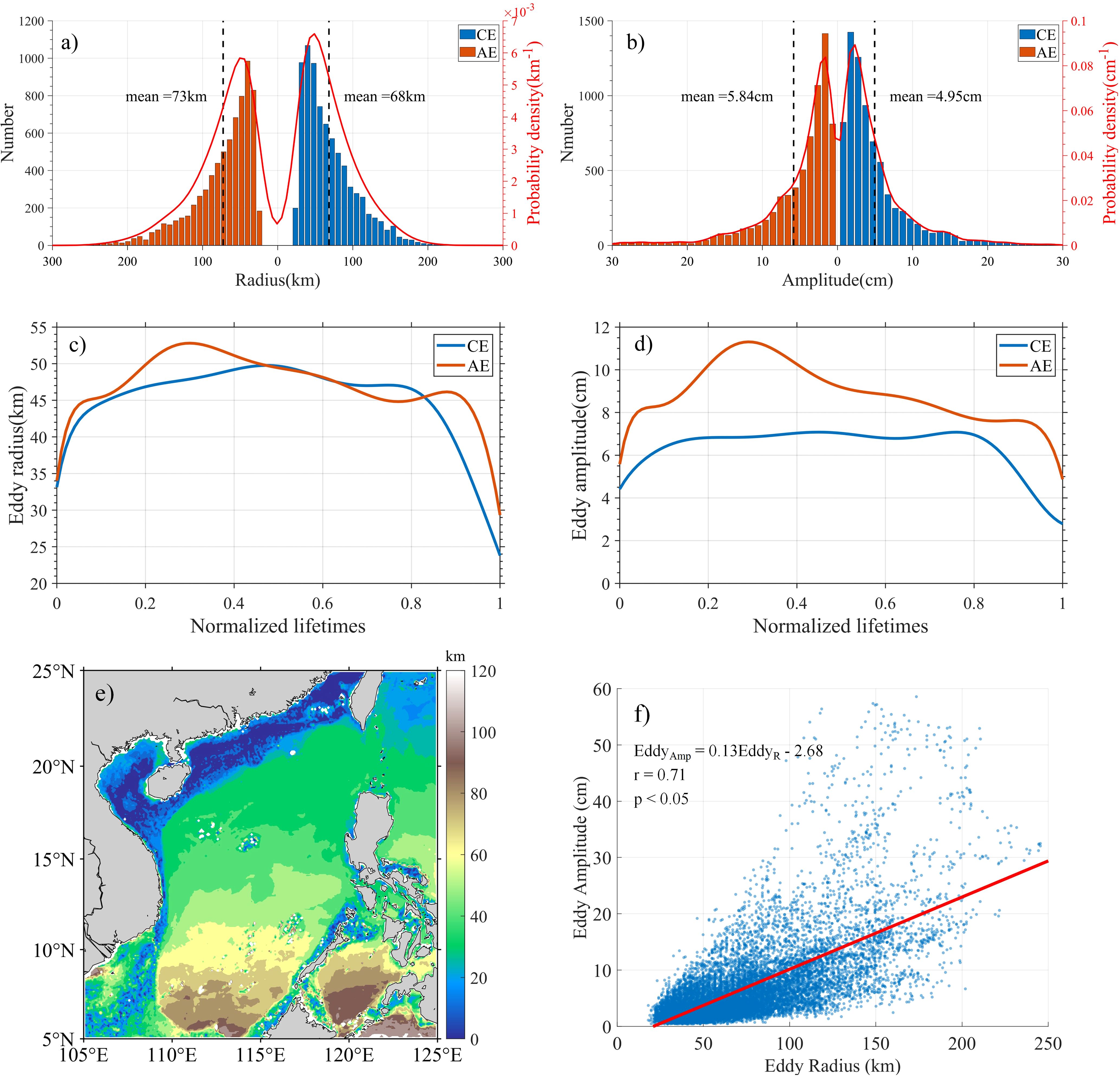
Figure 6. (a, b) Histogram and probability density curve of the radius and amplitude frequency distribution of mesoscale eddies in the SCS in 2021; (c, d) The normalized radius and amplitude evolution curves of mesoscale eddies in the SCS in 2021; (e) the deformation radius of the SCS baroclinic Rossby wave (L_R) calculated based on a simple two-layer model (the water body is divided into upper and lower layers by the thermocline boundary), $L_R=\frac{\sqrt{g^{\prime }H}}{f}$. where, $g^{\prime }=\frac{{\rho }_2-{\rho }_1}{{\rho }_1}g$, $H=\frac{H_1{H}_2}{H_1+H_2}$, $H_1$ and $H_2$are the thickness of the upper and lower water bodies; ${\rho }_1$ and ${\rho }_2$are the average density of the upper and lower water bodies, g is the gravitational acceleration; (f) the fitting curve of the mesoscale eddy radius and amplitude in the SCS in 2021.

In the SCS for 2021, cyclonic and anticyclonic mesoscale eddies exhibit similar trends in radius variation over their lifecycles, with consistent sizes during the same life phase (Figure 6c). During the middle to late stages (about 0.5~0.8 for normalized lifetime), there is a certain fluctuation in eddy radius, which does not follow a monotonic decay. In contrast, in the final stage (about from 0.8 or 0.9 for normalized lifetime), the eddy radius rapidly diminishes. Cyclonic eddy amplitudes are relatively smaller compared to anticyclonic ones during the same life phase (Figure 6d). Cyclonic eddies maintain a more stable and gradual variation throughout their lifecycle, with a rapid decrease only occurring at the end of their lifespan. In contrast, anticyclonic eddies experience a rapid increase in amplitude to a maximum value during the initial growth phase. Thus, there is a significant difference in amplitude between the two types of eddies at the beginning of their growth.

5 Discussion

5.1 More mesoscale eddy tracks recognized by YOLOv8 model

Figures 7a and b presents a comparative analysis of eddy tracks (with lifecycles exceeding four weeks) in the SCS, as identified by the PET method and the YOLOv8 model throughout 2021. The YOLOv8 model demonstrates a notable ability to track a substantial increase in eddy tracks in the central and southern SCS. Motion trajectories show that the majority of mesoscale eddies have a propensity for westward propagation. Conversely, some eddies exhibit a pronounced northward movement, particularly those influenced by the Kuroshio Current in the eastern part of the Luzon Strait. Additionally, there are eddies that appear to be trapped, indicating minimal spatial dispersion. For example, within the Sulu Sea, while eddies originating in the central and eastern areas predominantly move westward, those in the southern and western zones seem to be anchored in place, likely due to the geographical constraints imposed by the southwestern boundary of the Sulu Sea, hindering their westward propagation.

Figure 7

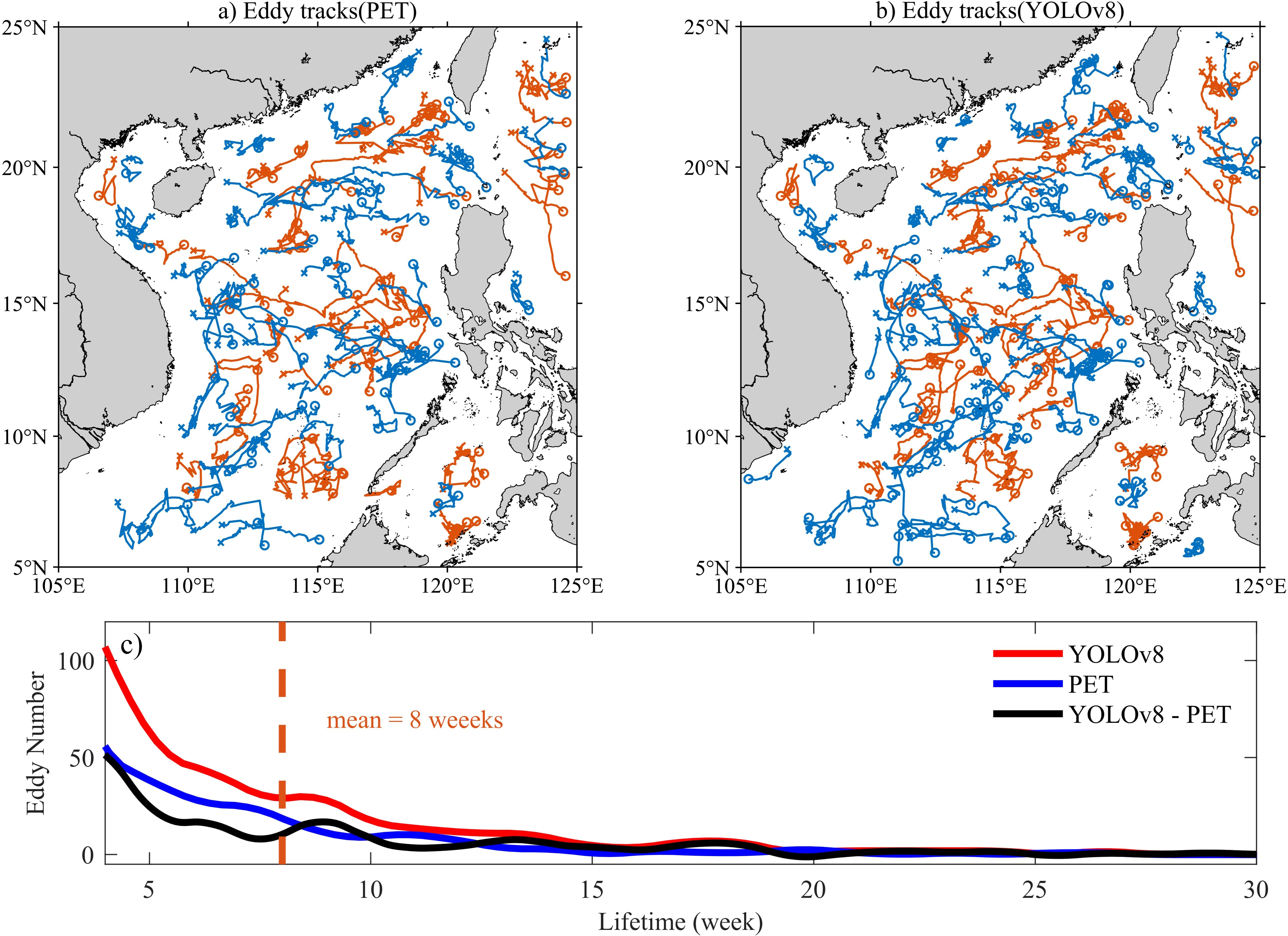
Figure 7. (a, b) Eddy tracks identified by PET method and YOLOv8 algorithm in the SCS in 2021 (life cycle greater than 4 weeks). Blue is cyclonic eddy track, and red is anticyclonic eddy track. ○ and × represent the locations where eddies were generated and dissipated. (c) Comparison of the number of eddy tracks (life cycle greater than 4 weeks) identified by PET method and YOLOv8 algorithm in 2021.

The number of eddy tracks recorded by the two methods (Figure 7c) reveals that, on average, mesoscale eddies with stable presence (lifecycles exceeding four weeks) in 2021 have a lifespan of about eight weeks. The YOLOv8 model excels in identifying eddy tracks with shorter lifecycles, uncovering over a hundred additional mesoscale eddy tracks with lifecycles ranging from four to eight weeks in 2021. The YOLOv8 model demonstrates a significant advantage over the PET method, detecting an average of 1 to 3 additional eddies per day in the SCS (Figure 5a). This enhanced performance can be primarily attributed to the superior generalization capabilities inherent in deep learning approaches, which are not limited by fixed physical thresholds. In the comparative analysis of mesoscale eddy tracking case (Figure 8), the PET method demonstrates a high degree of accuracy in identifying the contours of mesoscale eddies for most instances. However, this approach is contingent upon a fixed physical threshold for identification, which can lead to distortions in the shape of mesoscale eddies when the predicted threshold is not entirely applicable. For instance, as illustrated in Figure 8B, the identified anticyclonic eddy appears significantly smaller than its actual form. This limitation may also result in erroneous significant mutations in the characteristics of the eddy throughout its lifecycle. Moreover, the fixed threshold limitation of the PET method, especially the wide search interval, may cause it to miss some eddies during the identification process. As evidenced by Figures 8i–k, it can be inferred that an anticyclonic eddy persists based on ADT and sea surface geostrophic flow characteristics over these three days. Consequently, the identification results obtained from the YOLOv8 model are deemed to be reasonable. However, the PET method failed to detect this eddy consistently across those days, resulting in an abnormal interruption within its trajectory. Conversely, while boundary identification using the YOLOv8 algorithm is somewhat coarser compared to that achieved with PET, it effectively and accurately continues to identify the anticyclonic eddy over an extended period of eight days. The YOLOv8 model effectively addresses challenges such as rapid contour variations and shape deformations that occur during the dynamic evolution of mesoscale eddies. As a result, it identifies a greater number of eddies and establishes more comprehensive trajectories. During the propagation of mesoscale eddies, morphological variations can result in threshold deviations from the PET method; however, these eddies continue to persist. The YOLOv8 algorithm, characterized by its advanced generalization and robustness, effectively identifies these eddies. This capability prevents erroneous interruptions in trajectory tracking and facilitates a more precise monitoring of the complete lifecycle of mesoscale eddies. The YOLOv8 model’s threshold-free and generalized capabilities for detecting me-so-scale features will substantially enhance continuity in mesoscale trajectory tracking, thereby providing a more authentic and reliable trajectory dataset for research on mesoscale eddies.

Figure 8

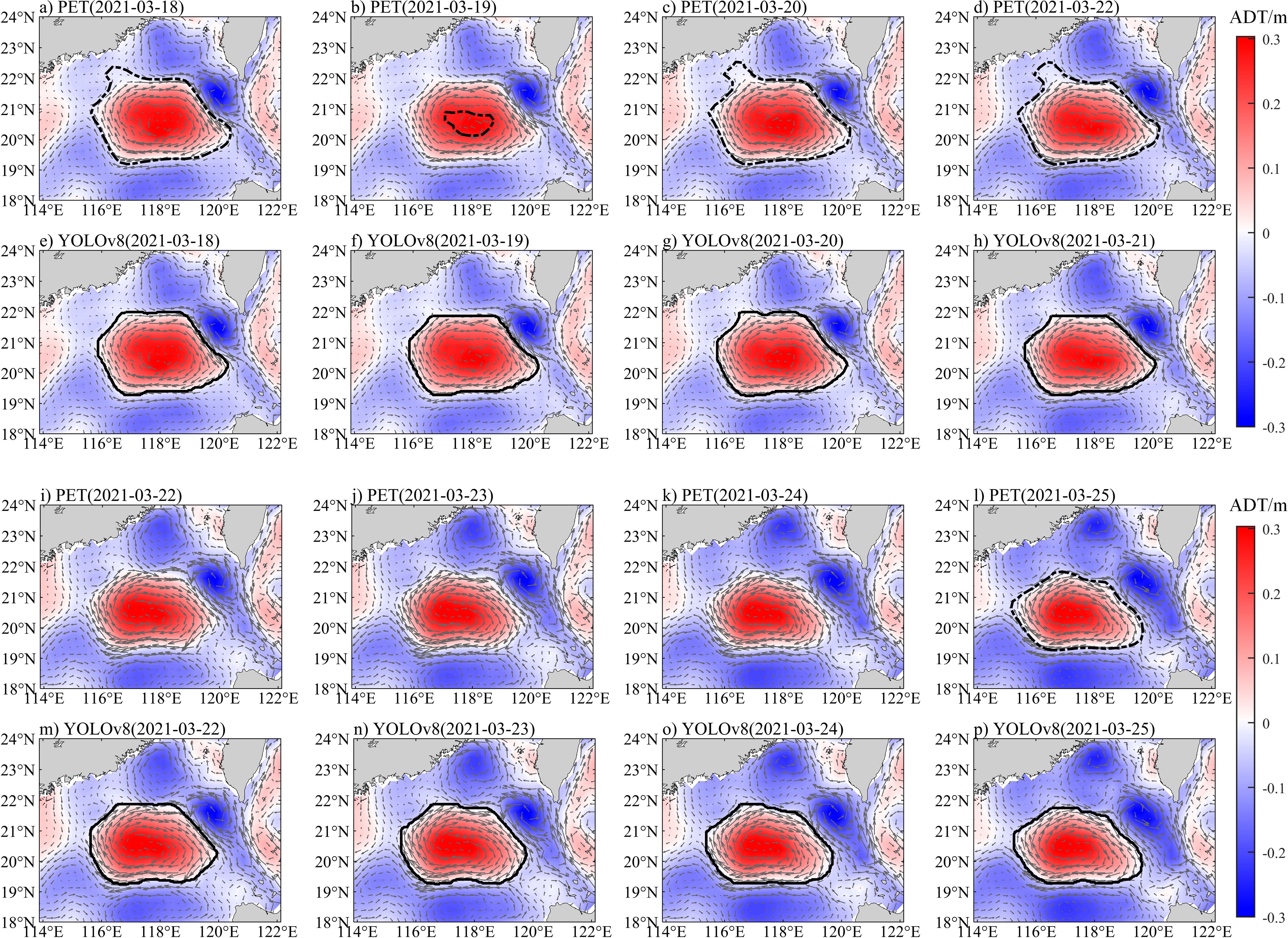
Figure 8. Comparison of eddy tracking case in the SCS (base map are the filtered ADT at 700km and sea surface geostrophic flow). (a–d) and (i–l) are the daily tracking effects of the PET method on an anticyclonic eddy in the northern SCS from March 18, 2021 to March 25, 2021, while (e–h) and (m–p) are the tracking effects of the YOLOv8 algorithm on the same anticyclonic eddy at the same time.

5.2 Tracking eddies changes under extreme events: a case study of typhoon Rai

Typhoon Rai formed in the low-latitude waters of the Northwest Pacific on December 13, 2021, and experienced a slow development phase initially. On December 16, 2021, the typhoon crossed the Philippines and entered the SCS. While in the SCS, Rai underwent two rapid intensifications, culminating in its development into a super typhoon. It gradually weakened and dissipated in the northern part of the SCS on December 21, 2021. The specific trajectory of Rai is detailed in Figure 9a. In the central SCS, Rai traversed four mesoscale eddies, comprising three cyclonic eddies and one anticyclonic eddy. After the passage of Rai, the sea under its path experienced a significant drop in SST (-0.5 to -1°C), as shown in Figure 9b. Data from Table 3 indicate that after the typhoon’s passage, the radii and amplitudes of the cyclonic eddies significantly increased, while the anticyclonic eddy notably weakened. On December 18 and 19, the typhoon successively passed over these four eddies. Post-typhoon on December 19, the radius of CE1 increased by 19.98 km and its amplitude by 2.48 cm; the radius of AE1 decreased by 6.88 km and its amplitude by 0.4 cm. These two eddies continued to exhibit trends of strengthening and weakening on December 20 and 21, respectively. The radii of CE2 and CE3 increased by 1.66 km and 12.59 km, respectively, and their amplitudes by 0.49 cm and 2.64 cm, respectively, but their radii and amplitudes gradually decreased over the following two days.

Figure 9

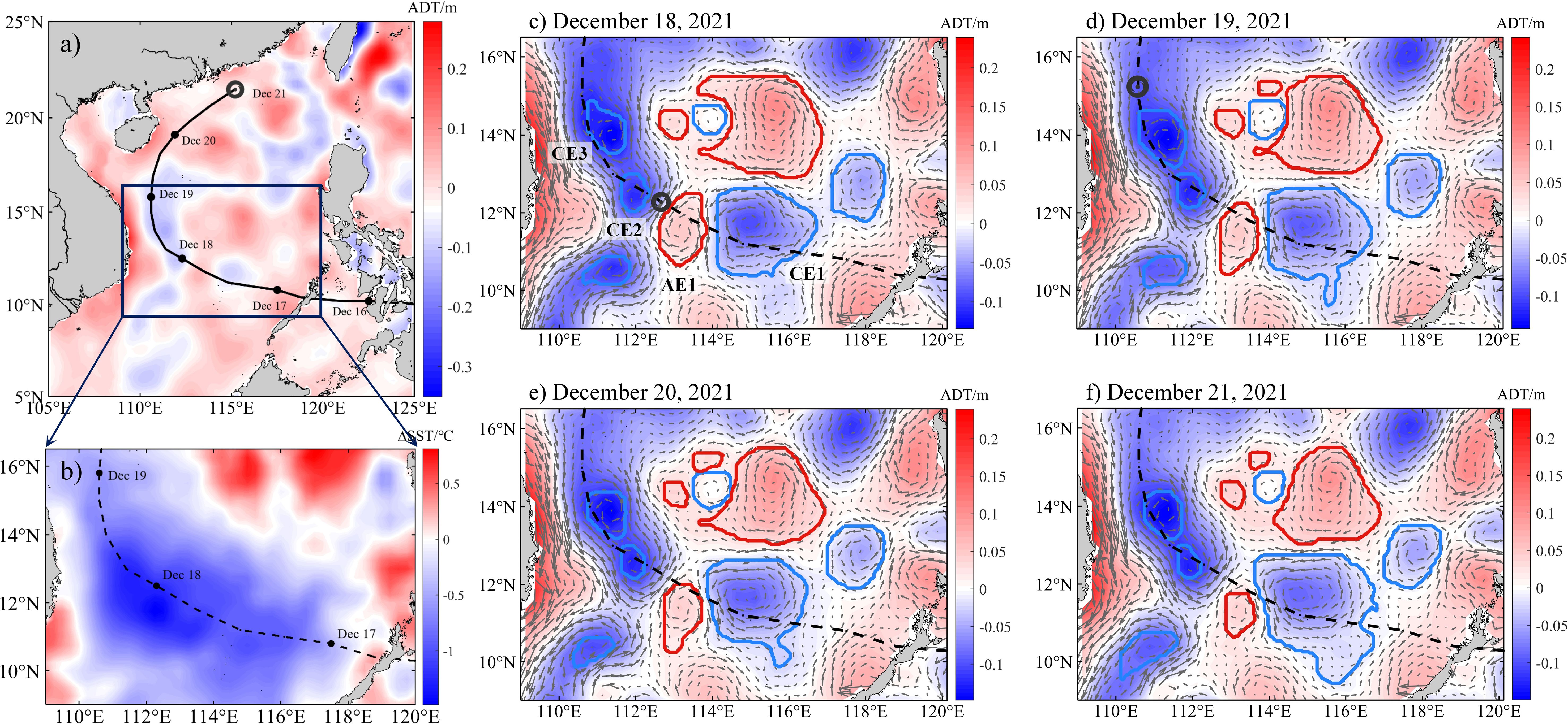
Figure 9. (a) The track of Typhoon "Rai" after entering the SCS. (b) The evolution of SST in the central SCS before and after Typhoon "Rai" entered (December 17, 2021) and left (December 20, 2021). (c–f) The evolution of mesoscale eddy characteristics in the central SCS following the passage of "Rai"(identification by YOLOv8).

Table 3

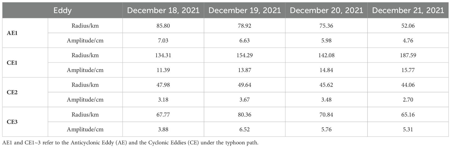
Table 3. The mesoscale eddy changes under the typhoon path identified by YOLOv8.

Recent studies on the interactions between typhoons and eddies have shown that when a typhoon traverses an eddy, the cyclonic eddy is typically amplified and its energy is intensified (Liu et al., 2017; Ma, 2020; Zhang et al., 2023). Conversely, the surface of the warm eddies (anticyclonic eddy usually) cools rapidly, resulting in a reduction of eddy energy, and it is more readily influenced by typhoons than cold eddies (cyclonic eddy usually). Furthermore, the characteristics of mesoscale eddy changes identified by YOLOv8 align with these conclusions.

This demonstrates that the YOLOv8 model maintains robust mesoscale eddy detection capabilities during extreme events, such as typhoons, accurately capturing eddy characteristics. Consequently, the YOLOv8 model serves as a reliable identification tool for studying mesoscale eddy variations under extreme conditions.

5.3 Comparisons of mesoscale eddy data sets

To further assess the performance of the YOLOv8 algorithm in identifying mesoscale eddies, this study compares the results of the YOLOv8 algorithm with two traditional mesoscale eddy datasets by using the SLA closed contour identification method (Base SLA) (Xu, 2021) and the Vector Geometry (VG) algorithm (Nencioli et al., 2010), respectively.

The YOLOv8 algorithm demonstrates superior capability in identifying mesoscale eddies relative to two conventional methods (Figure 10a), detecting nearly double the number of eddies identified by the Base SLA method. In contrast to YOLOv8, the Base SLA method sets minimum amplitude and radius thresholds for eddies and lacks spatial large-scale filtering on the input SLA field, leaving it vulnerable to interference from large-scale oceanic processes. Consequently, its ability to detect less prominent eddies is restricted, leading to a tendency to identify larger eddies while resulting in fewer overall detections. The distribution patterns of eddy radii and amplitudes identified by the YOLOv8 algorithm are similar to those identified by the VG method (Figures 10b, c). However, there is a slight decrease in the proportion of eddies with smaller radii and amplitudes, resulting in a more balanced identification outcome that better aligns with the actual conditions in the SCS. While, the VG method is based on closing the stream function field for identifying eddies, which yields consistent results with their characteristics. However, due to differences between flow field features and sea level height change features, this method does not account for sea level height variations caused by mesoscale eddies. As a result, it may lead to the identification of relatively smaller eddy radius.

Figure 10

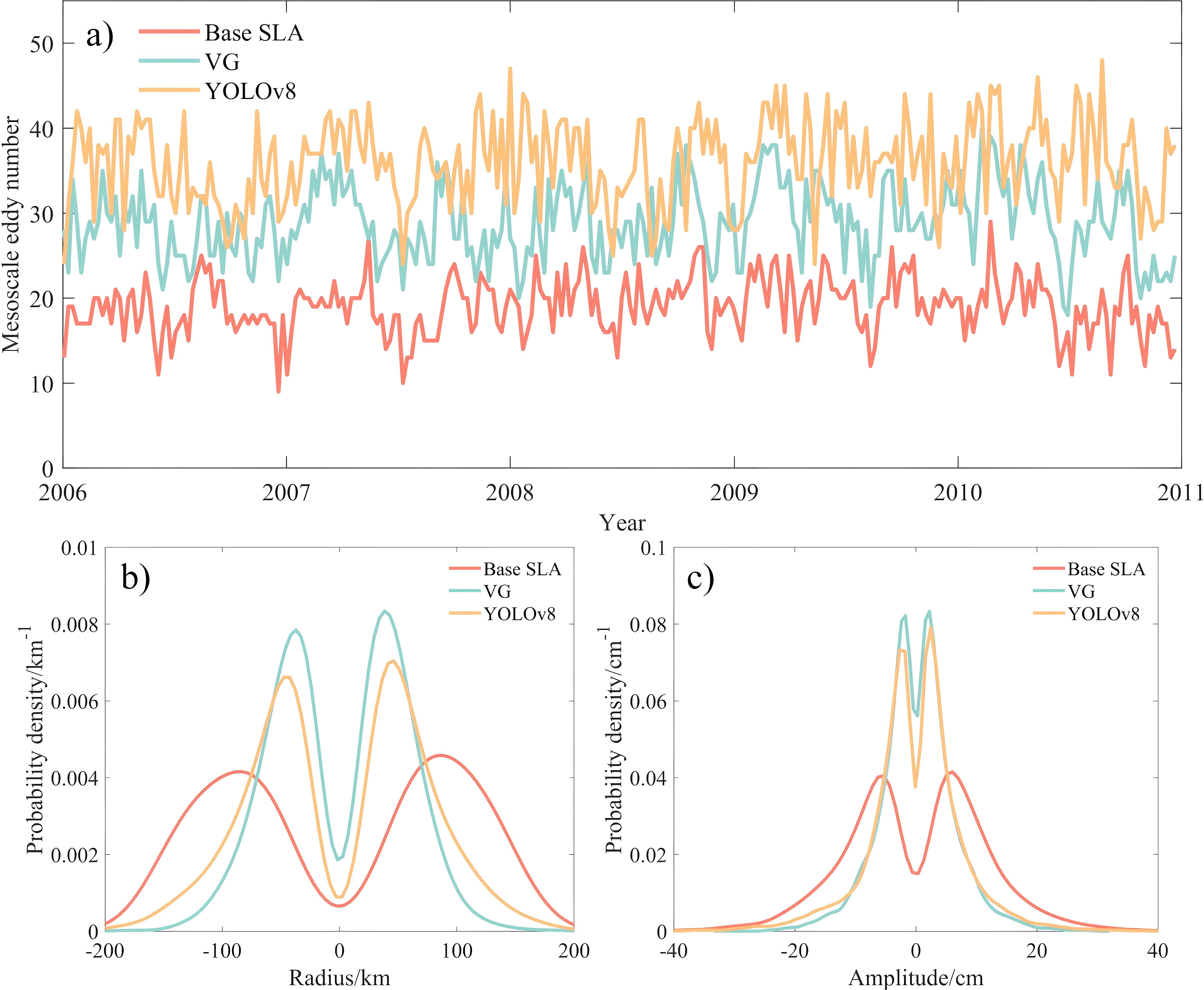
Figure 10. Comparisons of three eddy identification methods in the SCS from 2006 to 2020. (a) Mesoscale eddies numbers, (b) the probability density curve of eddy radius, and (c) the probability density curve of eddy amplitude. .

Results from January 3, 2006 (Figure 11) also indicate that the YOLOv8 algorithm exhibits superior capabilities in identifying a greater number of mesoscale eddies in the SCS when compared to these two methods. This indicates its superior performance in mesoscale eddy identification.

Figure 11

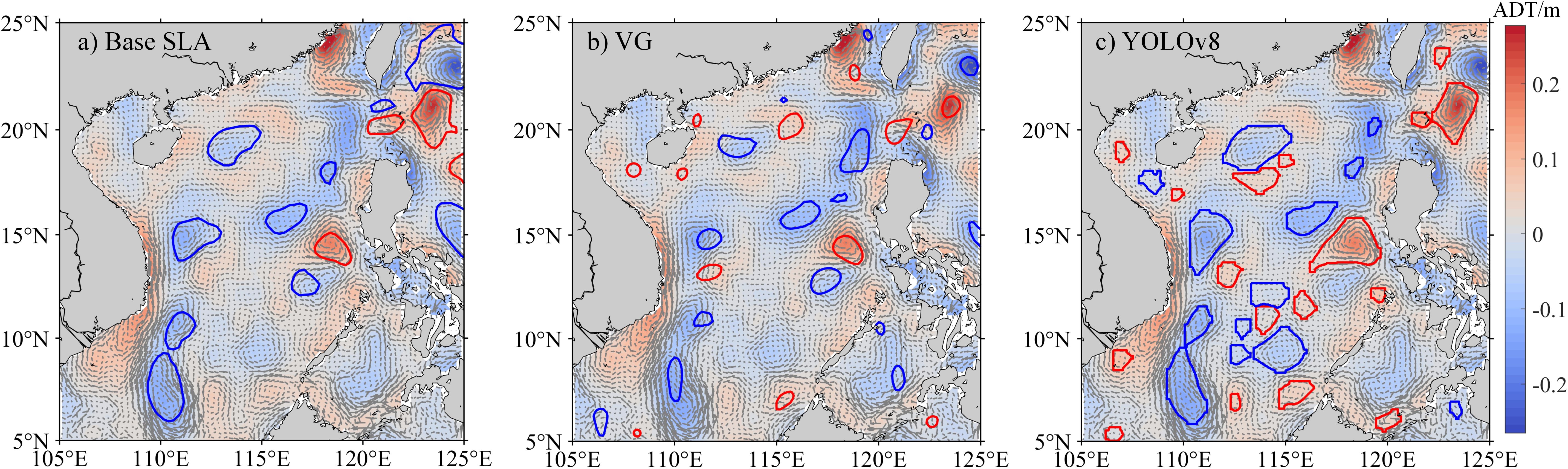
Figure 11. Eddy identification using three methods in the SCS on January 3, 2006. (a) Base SLA; (b) VG; (c) YOLOv8. The background map shows filtered ADT at 700km and sea surface geostrophic flow, with blue representing cyclonic eddies and red representing anticyclonic eddies.

5.4 Evaluation of YOLOv8’s generalization ability

5.4.1 Generalize to other seas: a case study of the Arabian Sea

The Arabian Sea and the SCS are located in similar latitudinal regions and experience comparable geostrophic effects, implying certain similarities in the meridional forces and Coriolis forces acting on the eddies. However, they exhibit significant differences in topography, monsoon patterns, and hydrodynamics. The Arabian Sea possesses a distinctive western boundary current, and due to the seasonal reversal of the Indian Ocean monsoon, the western boundary Somali Current shares this characteristic seasonal reversal (Fischer et al., 2002). Consequently, eddy activity in the Arabian Sea displays unique seasonal and spatial variations, which are markedly different from those in the SCS (Hammoud et al., 2023). Therefore, selecting the Arabian Sea as a test region for assessing the model’s generalization capability can effectively evaluate the model’s potential for broader application.

The four YOLOv8 models trained on the SCS dataset in section 4.2 were applied to identify mesoscale eddies in the Arabian Sea for the year 2021 (365 days), with the experimental results presented in Table 4. At the same time, we further analyze the recognition accuracy of the optimal results among the four models in different regions of the Arabian Sea, as shown in Figures 12g–i. The YOLOv8 model achieves an F1 score exceeding 85% across the entire Arabian Sea. However, in the central region of the sea, there is a relative decline in recognition rates for CE. This may be attributed to relatively stable ocean dynamics in this area, resulting in fewer occurrences of CE compared to other regions and increased difficulty due to weaker eddy characteristics (Trott et al., 2019). Additionally, in low-latitude marine areas, both CE and AE exhibit decreased recognition accuracy compared to that observed in the northern Arabian Sea. This could be due to the smaller scale and lower intensity of these eddies, which are more susceptible to zonal tensile deformation (Ni et al., 2020a, b), thereby increasing identification challenges.

Table 4

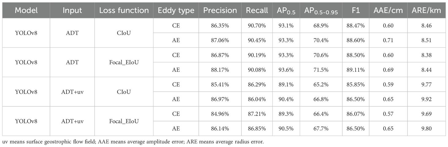
Table 4. Identification Effect of Mesoscale Eddies in the Arabian Sea.

Figure 12

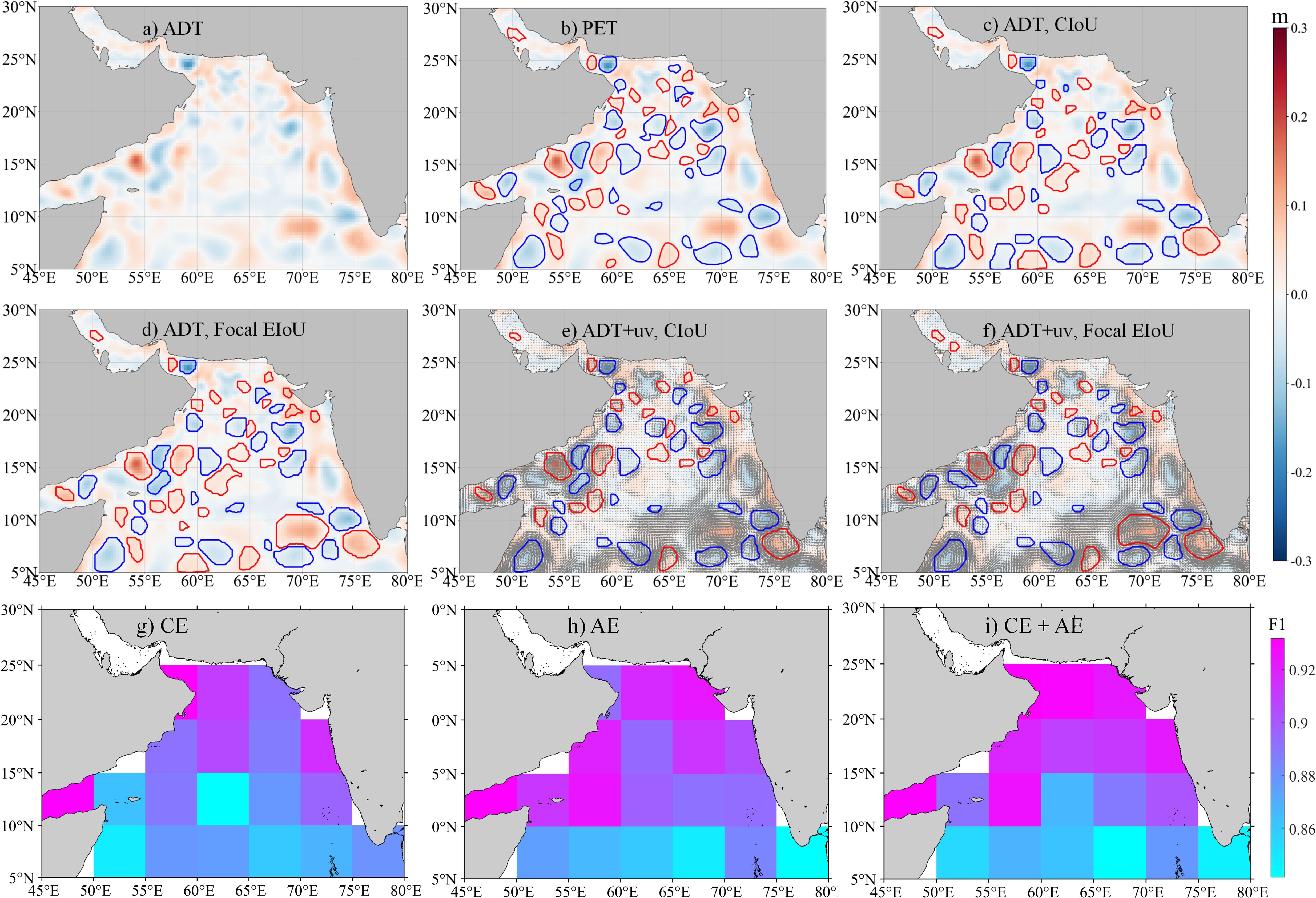
Figure 12. Transfer application of YOLOv8 models to the Arabian Sea on February 12, 2021. (a) filtered ADT at 700km; (b–f) the mesoscale eddies identification using PET method and the four YOLOv8 models trained for the SCS. Blue represents cyclonic eddies, and red represents anticyclonic eddies. (g–i) presents the cyclonic eddy, anticyclonic eddy, and overall eddy identification accuracies (F1 scores) in various regions obtained by the generalization of YOLOv8 to the Arabian Sea.

All four models demonstrate effective identification of mesoscale eddies in the Arabian Sea (Table 4). Notably, the YOLOv8 model utilizing only ADT as input, relative to the simultaneous input of ADT and uv, exhibits superior generalization capabilities. The YOLOv8 model, with an optimized loss function, achieves an average precision of 93.6% and an F1 score of 88.81% in identifying mesoscale eddies in the Arabian Sea. These results suggest that the deep learning model has strong generalization ability, enabling high-precision identification of mesoscale eddies across various marine dynamic environments. The relatively lower precision of the model using both ADT and uv input is due to the significant difference in sea surface current speeds between the South China Sea and the Arabian Sea. The faster coastal currents in the Arabian Sea create longer and denser vector arrows in the imagery, which obscure more ADT information compared to the SCS.

Figures 12a–f displays the transfer identification results of the four models on a particular day in the Arabian Sea. All models effectively identify mesoscale eddies in the new marine area and detect some eddies missed by the PET method. This indicates that the YOLOv8 model has captured the characteristic features of mesoscale eddies, retaining the ability to identify previously overlooked eddies in new marine areas. However, in areas with higher sea surface current speeds, the size of the mesoscale eddies identified by YOLOv8 appears relatively smaller than the actual size due to the obscuration of uv information.

In summary, the YOLOv8 model demonstrates robust transfer learning capabilities and could evolve into a new method for global mesoscale eddy identification.

5.4.2 Generalization to other resolution data products

Given that the ADT data from the Arabian Sea (in 5.3.1) is identical to the data product used for training the YOLOv8 model in the SCS, validating the model’s transferability and generalization by applying it to different data products for eddy identification is essential. The GLORYS12V1 product, offered by CMEMS, is a global ocean dataset with a 1/12° resolution that includes sea surface height (SSH) data. The higher resolution of this dataset compared to the ADT data used during model training allows for an effective assessment of YOLOv8’s adaptability to inputs of varying resolutions for mesoscale eddy identification.

Using the SSH data from GLORYS12V1, we calculated the SLA in the SCS for 2021, applied a 700 km filter, and then employed the YOLOv8 model trained in the SCS for identification. Table 5 compares the identification accuracy of the original YOLOv8 mesoscale eddy identification model with the new YOLOv8 model, which underwent an additional 10 epochs of training on GLORYS12V1 product data. Figure 13 shows the mesoscale eddies identification effect of both models on the same day.

Table 5

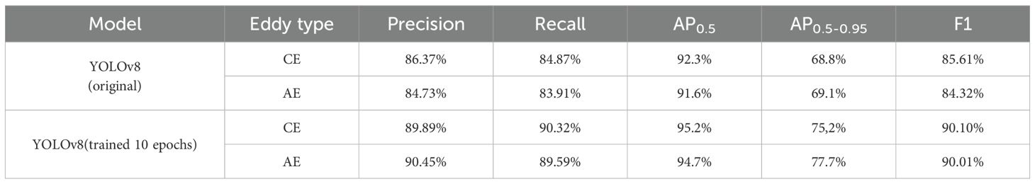
Table 5. The identification accuracy of mesoscale eddies in the SCS using the GLORYS12V1 data product.

Figure 13

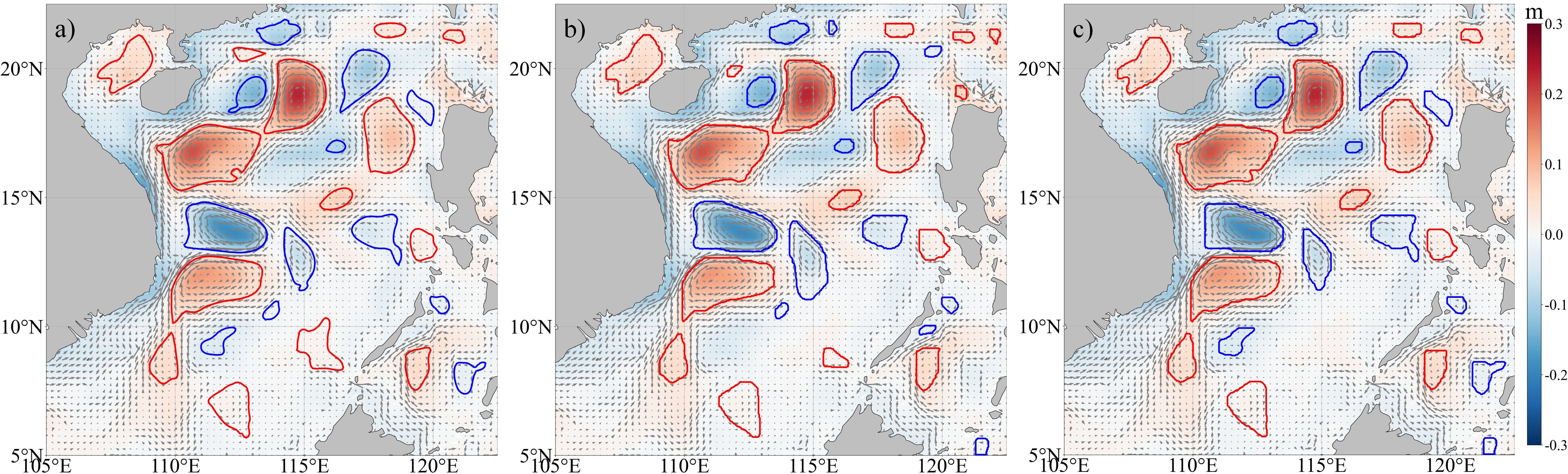
Figure 13. (a–c) Mesoscale eddy identification results of PET method, YOLOv8 (original), and YOLOv8 (trained 10 epochs) on the GLORYS12V1 data product on the same day in 2021.

Although the original YOLOv8 model’s accuracy dipped slightly when directly applied to identification compared to its initial performance, it still demonstrated robust capabilities, with a Recall of 84.39%, AP_0.5 of 91.9%, and an F1 score of 84.97%. These identification results align well with the PET method, meeting the detection requirements for mesoscale eddies and showcasing the model’s generalization and versatility. The slight decrease in accuracy is attributed to the higher spatial resolution of the input data, which provides the algorithm with more nuanced information, some of which the original model had not encountered. Moreover, after an additional 10 epochs of training on the new product data, the model’s identification accuracy significantly improved: Recall rose to 89.96%, AP_0.5 to 94.9%, and the F1 score to 90.05%. Thus, when transitioning to different data sources for mesoscale eddy identification, enhancing the accuracy of the existing YOLOv8 model requires only minimal additional training.

In conclusion, YOLOv8 has exhibited formidable transfer learning capabilities, whether detecting mesoscale eddies in various waters or employing different data products, suggesting its potential as a novel global method for mesoscale eddy detection.

6 Conclusion

This study uses ADT data from AVISO and the improved YOLOv8 algorithmic model to conduct a mesoscale eddy identification study in the South China Sea (5°~25°N, 105~125°E). By adjusting input data, refining the model’s loss function, and performing transfer learning tests, the study reaches several conclusions:

1. YOLOv8 achieves high-precision identification of mesoscale eddies in the in the SCS, with Recall of 94%, AP_0.5 of 96%, F1 of 90%, average radius error below 5 km, and average amplitude error below 0.50 cm.

2. Incorporating sea surface current field information enhances eddy characteristics, improving model accuracy. However, some ADT information obscuration leads to slightly increased errors in amplitude and radius.

3. YOLOv8 can detect some mesoscale eddies undetected by the PET model and track more mesoscale eddy trajectories, offering a dataset that is richer in eddy quantity.

4. In extreme events such as typhoons, YOLOv8 maintains its ability to accurately identify the characteristic changes of mesoscale eddies, showing high reliability.

5. The YOLOv8 model trained in the SCS achieves high-precision identification in the Arabian Sea (Recall 90.5%, AP_0.5 93.6%) and retains accuracy when transferred to high-resolution data (Recall 84.39%, AP_0.5 91.9%). With additional training on this dataset for 10 epochs, accuracy can be enhanced (Recall 89.96%, AP_0.5 94.9%). Consequently, the YOLOv8 demonstrates robust generalization and applicability across various maritime regions and data products.

Deep learning methods, as a novel approach to target identification, can effectively identify mesoscale oceanic eddies. ADT is not merely a variable in marine elements; it also includes physical information such as the cumulative effects of air-sea dynamics and historical information. Deep learning methods begin with the data, extract and learn the implicit information behind it, and match it with the characteristics of mesoscale eddies to achieve efficient and precise identification. This study provides a new deep learning method for the mesoscale eddies identification and provides more refined and comprehensive mesoscale eddies trajectory data for the studying their formation and dissipation processes.

Data availability statement

The original contributions presented in the study are included in the article/supplementary material. Further inquiries can be directed to the corresponding authors.

Author contributions

JG: Conceptualization, Data curation, Formal Analysis, Investigation, Methodology, Software, Visualization, Writing – original draft, Writing – review & editing. FZ: Conceptualization, Formal Analysis, Funding acquisition, Investigation, Supervision, Writing – review & editing. DT: Conceptualization, Formal Analysis, Funding acquisition, Methodology, Supervision, Writing – original draft, Writing – review & editing. MZ: Formal Analysis, Investigation, Methodology, Writing – original draft. HG: Project administration, Supervision, Writing – original draft.

Funding

The author(s) declare that financial support was received for the research and/or publication of this article. National Natural Science Foundation of China (Grant No. U23A2033), the Key R&D Program of Zhejiang Province (Grant No. 2024C03034, 2024C03257), National Natural Science Foundation of China (Grant No. 42106010) and Ocean Decade Project (Kuroshio Edge Exchange and the Shelf Ecosystem, Grant No. CSK-2/08/2023).

Conflict of interest

The authors declare that the research was conducted in the absence of any commercial or financial relationships that could be construed as a potential conflict of interest.

Generative AI statement

The author(s) declare that no Generative AI was used in the creation of this manuscript.

Publisher’s note

All claims expressed in this article are solely those of the authors and do not necessarily represent those of their affiliated organizations, or those of the publisher, the editors and the reviewers. Any product that may be evaluated in this article, or claim that may be made by its manufacturer, is not guaranteed or endorsed by the publisher.

References

Ashkezari M. D., Hill C. N., Follett C. N., Forget G., Follows M. J. (2016). Oceanic eddy detection and lifetime forecast using machine learning methods. Geophysical Res. Lett. 43, 12234–12241. doi: 10.1002/2016GL071269

Crossref Full Text | Google Scholar

Cao L. J., Zhang D. N., Zhang X. F., Guo Q. (2022). Detection and identification of mesoscale eddies in the south China sea based on an artificial neural network model-YOLOF and remotely sensed data. Remote Sens. 14, 19. doi: 10.3390/rs14215411

Crossref Full Text | Google Scholar

Chaigneau A., Le Texier M., Eldin G., Grados C., Pizarro O. (2011). Vertical structure of mesoscale eddies in the eastern South Pacific Ocean: A composite analysis from altimetry and Argo profiling floats. J. Geophysical Research: Oceans 116, C11025. doi: 10.1029/2011JC007134

Crossref Full Text | Google Scholar

Chelton D. B., Schlax M. G., Samelson R. M. (2011). Global observations of nonlinear mesoscale eddies. Prog. Oceanography 91, 167–216. doi: 10.1016/j.pocean.2011.01.002

Crossref Full Text | Google Scholar

Chen G. X., Hou Y. J., Chu X. Q. (2011). Mesoscale eddies in the South China Sea: Mean properties, spatiotemporal variability, and impact on thermohaline structure. J. Geophysical Research: Oceans 116, C06018. doi: 10.1029/2010JC006716

Crossref Full Text | Google Scholar

Chu P. C., Edmons N. L., Fan C. W. (1999). Dynamical mechanisms for the South China Sea seasonal circulation and thermohaline variabilities. J. Phys. Oceanography 29, 2971–2989. doi: 10.1175/1520-0485(1999)029<2971:DMFTSC>2.0.CO;2

Crossref Full Text | Google Scholar

Dong C. M., McWilliams J. C., Liu Y., Chen D. K. (2014). Global heat and salt transports by eddy movement. Nat. Commun. 5, 3294. doi: 10.1038/ncomms4294

PubMed Abstract | Crossref Full Text | Google Scholar

Dong D., Brandt P., Chang P., Schutte F., Yang X. F., Yan J. H., et al. (2017). Mesoscale eddies in the northwestern pacific ocean: three-dimensional eddy structures and heat/salt transports. J. Geophysical Research: Oceans 122, 9795–9813. doi: 10.1002/2017JC013303

Crossref Full Text | Google Scholar

Fischer A. S., Weller R. A., Rudnick D. L., Eriksen C. C., Lee C. M., Brink K. H., et al. (2002). Mesoscale eddies, coastal upwelling, and the upper-ocean heat budget in the Arabian Sea. Deep Sea Res. Part II: Topical Stud. Oceanography 49, 2231–2264. doi: 10.1016/S0967-0645(02)00036-X

Crossref Full Text | Google Scholar

Frenger I., Gruber N., Knutti R., Munnich M. (2013). Imprint of Southern Ocean eddies on winds, clouds and rainfall. Nat. Geosci. 6, 608–612. doi: 10.1038/NGEO1863

Crossref Full Text | Google Scholar

Gaube P., McGillicuddy D. J., Moulin A. J. (2019). Mesoscale eddies modulate mixed layer depth globally. Geophysical Res. Lett. 46, 1505–1512. doi: 10.1029/2018GL080006

Crossref Full Text | Google Scholar

Guo M. X., Xiu P., Li S. Y., Chai F., Xue H. J., Zhou K. B., et al. (2017). Seasonal variability and mechanisms regulating chlorophyll distribution in mesoscale eddies in the South China Sea. J. Geophysical Research: Oceans 122, 5329–5347. doi: 10.1002/2016JC012670

Crossref Full Text | Google Scholar

Hammoud M. A. E., Zhan P., Hakla O., Knio O., Hoteit I. (2023). Semantic segmentation of mesoscale eddies in the arabian sea: A deep learning approach. Remote Sens. 15, 17. doi: 10.3390/rs15061525

Crossref Full Text | Google Scholar

Jalal A., Salman A., Mian A., Shortis M., Shafait F. (2020). Fish detection and species classification in underwater environments using deep learning with temporal information. Ecol. Inf. 57, 101088. doi: 10.1016/j.ecoinf.2020.101088

Crossref Full Text | Google Scholar

Jeong J., Hussain F. (1995). On the identification of a vortex. J. Fluid Mechanics 285, 69–94. doi: 10.1017/S0022112095000462

Crossref Full Text | Google Scholar

Jia Y. L., Chassignet E. P. (2011). Seasonal variation of eddy shedding from the Kuroshio intrusion in the Luzon Strait. J. Oceanography 67, 601–611. doi: 10.1007/s10872-011-0060-1

Crossref Full Text | Google Scholar

Jocher G., Chaurasia A., Qiu J. (2023). Ultralytics YOLO (GitHub). Available online at: https://github.com/ultralytics/ultralytics (Accessed April 19, 2023).

Google Scholar

Kavitha A. R., Palaniappan K. (2023). Brain tumor segmentation using a deep Shuffled-YOLO network. Int. J. Of Imaging Syst. Technol. 33, 511–522. doi: 10.1002/ima.22832

Crossref Full Text | Google Scholar

Levy M. (2003). Mesoscale variability of phytoplankton and of new production: Impact of the large-scale nutrient distribution (Journal of Geophysical Research: Oceans 108(C11). doi: 10.1029/2002JC001577

Crossref Full Text | Google Scholar

Lguensat R., Sun M., Fablet R., Mason E., Tandeo P., Chen G., et al. (2018). “EddyNet: A deep neural network for pixel-wise classification of oceanic eddies,” in IGARSS 2018 - 2018 IEEE International Geoscience and Remote Sensing Symposium, Valencia, Spain, pp. 1764–1767. doi: 10.1109/IGARSS.2018.8518411

Crossref Full Text | Google Scholar

Li B. X., Tang H., Ma D. F., Lin J. M. (2022). A dual-attention mechanism deep learning network for mesoscale eddy detection by mining spatiotemporal characteristics. J. Atmospheric Oceanic Technol. 39, 1115–1128. doi: 10.1175/jtech-d-21-0128.1

Crossref Full Text | Google Scholar

Li X., Wang W., Wu L., Chen S., Hu X., Li J., et al. (2020). Generalized focal loss: Learning qualified and distributed bounding boxes for dense object detection. Adv Neural Inf Process Syst. 33, 21002–21012. Available online at: https://proceedings.neurips.cc/paper_files/paper/2020/hash/f0bda020d2470f2e74990a07a607ebd9-Abstract.html

Google Scholar

Liu Q. L., Gong X. Y., Li J., Wang H. J., Liu R., Liu D., et al. (2023). A multitask model for realtime fish detection and segmentation based on YOLOv5. Peerj Comput. Sci. 9, e1262. doi: 10.7717/peerj-cs.1262

PubMed Abstract | Crossref Full Text | Google Scholar

Liu C., Lin X., Xu G., Han G., Liu Y. (2024). Improved identification and tracking of three-dimensional eddies in the Southern Ocean utilizing 3D-U-Res-Net. Front. Mar. Sci. 11. doi: 10.3389/fmars.2024.1482804

Crossref Full Text | Google Scholar

Liu J. Q., Piao S. C., Gong L. J., Zhang M. H., Guo Y. C., Zhang S. Z. (2021). The effect of mesoscale eddy on the characteristic of sound propagation. J. Mar. Sci. Eng. 9, 787. doi: 10.3390/jmse9080787

Crossref Full Text | Google Scholar

Liu S.-S., Sun L., Wu Q., Yang Y.-J. (2017). The responses of cyclonic and anticyclonic eddies to typhoon forcing: The vertical temperature-salinity structure changes associated with the horizontal convergence/divergence. J. Geophysical Research: Oceans 122, 4974–4989. doi: 10.1002/2017JC012814

Crossref Full Text | Google Scholar

Liu C. Q., Wang Y. Q., Yang Y., Duan Z. W. (2016). New omega vortex identification method. Science China: Physics, Mechanics and Astronomy 59, 684–711. doi: 10.1007/s11433-016-0022-6

Crossref Full Text | Google Scholar

Ma Z. (2020). A study of the interaction between typhoon francisco, (2013) and a cold-core eddy. Part I: rapid weakening. J. Atmospheric Sci. 77, 355–377. doi: 10.1175/JAS-D-18-0378.1

Crossref Full Text | Google Scholar

Mason E., Pascual A., McWilliams J. C. (2014). A new sea surface height-based code for oceanic mesoscale eddy tracking. J. Atmospheric Oceanic Technol. 31, 1181–1188. doi: 10.1175/JTECH-D-14-00019.1

Crossref Full Text | Google Scholar

McGillicuddy D. J., Robinson A. R., Siegel D. A., Jannasch H. W., Johnson R., Dickeys T., et al. (1998). Influence of mesoscale eddies on new production in the Sargasso Sea. Nature 394, 263–266. doi: 10.1038/28367

Crossref Full Text | Google Scholar

Nan F., Xue H. J., Yu F. (2015). Kuroshio intrusion into the South China Sea: A review. Prog. In Oceanography 137, 314–333. doi: 10.1016/j.pocean.2014.05.012

Crossref Full Text | Google Scholar

Nencioli F., Dong C. M., Dickey T., Washburn L., McWilliams J. C. (2010). A vector geometry-based eddy detection algorithm and its application to a high-resolution numerical model product and high-frequency radar surface velocities in the southern california bight. J. Atmospheric Oceanic Technol. 27, 564–579. doi: 10.1175/2009JTECHO725.1

Crossref Full Text | Google Scholar

Ni Q. B., Zhai X. M., Wang G. H., Hughes C. W. (2020b). Widespread mesoscale dipoles in the global ocean. J. Geophysical Research: Oceans 125, e2020JC016479. doi: 10.1029/2020JC016479

Crossref Full Text | Google Scholar

Ni Q., Zhai X., Wang G., Marshall D. P. (2020a). Random movement of mesoscale eddies in the global ocean. J. Phys. Oceanography 50, 2341–2357. doi: 10.1175/JPO-D-19-0192.1

Crossref Full Text | Google Scholar

Oka E., Toyama K., Suga T. (2009). Subduction of North Pacific central mode water associated with subsurface mesoscale eddy. Geophysical Res. Lett. 36, L08607. doi: 10.1029/2009GL037540

Crossref Full Text | Google Scholar

Okubo A. (1970). Horizontal dispersion of floatable particles in vicinity of velocity singularities such as convergences. Deep-sea Res. 17, 445. doi: 10.1016/0011-7471(70)90059-8

Crossref Full Text | Google Scholar

Pegliasco C., Delepoulle A., Mason E., Morrow R., Faugere Y., Dibarboure G. (2022). META3.1exp: a new global mesoscale eddy trajectory atlas derived from altimetry. Earth System Sci. Data 14, 1087–1107. doi: 10.5194/essd-14-1087-2022

Crossref Full Text | Google Scholar

Redmon J., Divvala S., Girshick R., Farhadi A., Ieee (2016). “You only look once: unified, real-time object detection,” in 2016 IEEE Conference on Computer Vision and Pattern Recognition (CVPR), Las Vegas, NV, USA, 2016, pp. 779–788. doi: 10.1109/CVPR.2016.91

Crossref Full Text | Google Scholar

Sadarjoen I. A., Post F. H. (2000). Detection, quantification, and tracking of vortices using streamline geometry. Comput. Graphics-UK 24, 333–341. doi: 10.1016/S0097-8493(00)00029-7

Crossref Full Text | Google Scholar

Saida S. J., Ari S. (2022). MU-net: modified U-net architecture for automatic ocean eddy detection. IEEE Geosci. Remote Sens. Lett. 19, 1–5. doi: 10.1109/LGRS.2022.3225140

Crossref Full Text | Google Scholar

Trott C. B., Subrahmanyam B., Chaigneau A., Roman-Stork H. L. (2019). Eddy-induced temperature and salinity variability in the Arabian sea. Geophysical Res. Lett. 46, 2734–2742. doi: 10.1029/2018GL081605

Crossref Full Text | Google Scholar

Uchida T., Deremble B., Popinet S. (2022). Deterministic model of the eddy dynamics for a midlatitude ocean model. J. Phys. Oceanography 52, 1133–1154. doi: 10.1175/JPO-D-21-0217.1

Crossref Full Text | Google Scholar

van Westen R. M., Dijkstra H. A. (2021). Ocean eddies strongly affect global mean sea-level projections. Sci. Adv. 7, eabf1674. doi: 10.1126/sciadv.abf1674

PubMed Abstract | Crossref Full Text | Google Scholar

Wang G. H., Li J. X., Wang C. Z., Yan Y. W. (2012a). Interactions among the winter monsoon, ocean eddy and ocean thermal front in the South China Sea. J. Geophysical Research: Oceans 117, C08002. doi: 10.1029/2012JC008007

Crossref Full Text | Google Scholar

Wang S. H., Song Z. Y., Ma W. D., Shu Q., Qiao F. L. (2022a). Mesoscale and submesoscale turbulence in the Northwest Pacific Ocean revealed by numerical simulations. Deep Sea Res. Part II: Topical Stud. Oceanography 206, 105221. doi: 10.1016/j.dsr2.2022.105221

Crossref Full Text | Google Scholar

Wang X. N., Wang X. G., Li C., Zhao Y. B., Ren P. (2022b). Data-attention-YOLO (DAY): A comprehensive framework for mesoscale eddy identification. Pattern Recognition 131, 16. doi: 10.1016/j.patcog.2022.108870

Crossref Full Text | Google Scholar

Wang H., Wang D. K., Liu G. M., Wu H. D., Li M. (2012b). Seasonal variation of eddy kinetic energy in the South China Sea. Acta Oceanologica Sin. 31, 1–15. doi: 10.1007/s13131-012-0170-7

Crossref Full Text | Google Scholar

Weiss J. (1991). The dynamics of enstrophy transfer in 2-dimensional hydrodynamics. Physica D: Nonlinear Phenomena 48, 273–294. doi: 10.1016/0167-2789(91)90088-Q

Crossref Full Text | Google Scholar

Wu C. R., Chiang T. L. (2007). Mesoscale eddies in the northern South China Sea. Deep Sea Res. Part II: Topical Stud. Oceanography 54, 1575–1588. doi: 10.1016/j.dsr2.2007.05.008

Crossref Full Text | Google Scholar

Xia Q., Shen H. (2015). Automatic detection of oceanic mesoscale eddies in the South China Sea. Chin. J. Oceanology Limnology 33, 1334–1348. doi: 10.1007/s00343-015-4354-9

Crossref Full Text | Google Scholar

Xie H., Xu Q., Dong C. (2024). Deep learning for mesoscale eddy detection with feature fusion of multisatellite observations. IEEE J. Selected Topics Appl. Earth Observations Remote Sens. 17, 18351–18364. doi: 10.1109/JSTARS.2024.3468457

Crossref Full Text | Google Scholar

Xiu P., Chai F. (2020). Eddies affect subsurface phytoplankton and oxygen distributions in the north pacific subtropical gyre. Geophysical Res. Lett. 47, e2020GL087037. doi: 10.1029/2020GL087037

Crossref Full Text | Google Scholar

Xu C. (2021). Simple eddy detection (GitHub). Available at: https://github.com/chouj/SimpleEddyDetection (Accessed July 14, 2024).

Google Scholar

Xu G. K., Xie W. H., Dong C. M., Gao X. Q. (2021). Application of three deep learning schemes into oceanic eddy detection. Front. Mar. Sci. 8. doi: 10.3389/fmars.2021.672334

Crossref Full Text | Google Scholar

Xu G., Xie W., Lin X., Liu Y., Hang R., Sun W., et al. (2024). Detection of three-dimensional structures of oceanic eddies using artificial intelligence. Ocean Model. 190, 102385. doi: 10.1016/j.ocemod.2024.102385

Crossref Full Text | Google Scholar

Xue B., Huang B. X., Chen G., Li H. T., Wei W. B. (2021). Deep-sea debris identification using deep convolutional neural networks. IEEE J. Of Selected Topics In Appl. Earth Observations And Remote Sens. 14, 8909–8921. doi: 10.1109/JSTARS.2021.3107853

Crossref Full Text | Google Scholar

Yang Z. B., Jing Z., Zhai X. M. (2022). Effect of small-scale topography on eddy dissipation in the northern south China sea. J. Phys. Oceanography 52, 2397–2416. doi: 10.1175/JPO-D-21-0208.1

Crossref Full Text | Google Scholar

Yang Y. K., Wang D. X., Wang Q., Zeng L. L., Xing T., He Y. K., et al. (2019). Eddy-induced transport of saline kuroshio water into the northern south China sea. J. Geophysical Research: Oceans 124, 6673–6687. doi: 10.1029/2018JC014847

Crossref Full Text | Google Scholar

Zhang H., Liu Y., Liu P., Guan S., Wang Q., Zhao W., et al. (2023). Enhanced upper ocean response within a warm eddy to Typhoon Nakri, (2019) during the sudden-turning stage. Deep Sea Res. Part I: Oceanographic Res. Papers 199, 104112. doi: 10.1016/j.dsr.2023.104112

Crossref Full Text | Google Scholar

Zhang Y. Y., Liu N., Zhang Z. Y., Liu M., Fan L., Li Y. B., et al. (2022b). Detection of bering sea slope mesoscale eddies derived from satellite altimetry data by an attention network. Remote Sens. 14, 13. doi: 10.3390/rs14194974

Crossref Full Text | Google Scholar

Zhang X., Pan X., Zhu R., Guan R., Qiu Z., Song B. (2024). Faster AMEDA—A hybrid mesoscale eddy detection algorithm. Comput. Modeling Eng. Sci. 141, 1827–1846. doi: 10.32604/cmes.2024.054298

Crossref Full Text | Google Scholar

Zhang Z. G., Qiu B. (2018). Evolution of submesoscale ageostrophic motions through the life cycle of oceanic mesoscale eddies. Geophysical Res. Lett. 45, 11847–11855. doi: 10.1029/2018GL080399

Crossref Full Text | Google Scholar

Zhang Y. F., Ren W. Q., Zhang Z., Jia Z., Wang L., Tan T. N. (2022a). Focal and efficient IOU loss for accurate bounding box regression. Neurocomputing 506, 146–157. doi: 10.1016/j.neucom.2022.07.042

Crossref Full Text | Google Scholar

Zhang Z. G., Wang W., Qiu B. (2014). Oceanic mass transport by mesoscale eddies. Science 345, 322–324. doi: 10.1126/science.1252418

PubMed Abstract | Crossref Full Text | Google Scholar

Zhang T. W., Zhang X. L. (2019). High-speed ship detection in SAR images based on a grid convolutional neural network. Remote Sens. 11, 1206. doi: 10.3390/rs11101206

Crossref Full Text | Google Scholar

Zhao N., Huang B. X., Yang J., Radenkovic M., Chen G. (2023). Oceanic eddy identification using pyramid split attention U-net with remote sensing imagery. IEEE Geosci. Remote Sens. Lett. 20, 5. doi: 10.1109/lgrs.2023.3243902

Crossref Full Text | Google Scholar

Zheng Z. H., Wang P., Liu W., Li J. Z., Ye R. G., Ren D. W., et al. (2020). “Distance-ioU loss: faster and better learning for bounding box regression,” in The Thirty-Second AAAI Conference on Artificial Intelligence. 34, 12993–13000. doi: 10.1609/aaai.v34i07.6999

Crossref Full Text | Google Scholar

Zhou J., Zhou G. D., Liu H. L., Li Z. H., Cheng X. H. (2021). Mesoscale eddy-induced ocean dynamic and thermodynamic anomalies in the north pacific. Front. In Mar. Sci. 8. doi: 10.3389/fmars.2021.756918

Crossref Full Text | Google Scholar

Zi N., Li X.-M., Gade M., Fu H., Min S. (2024). Ocean eddy detection based on YOLO deep learning algorithm by synthetic aperture radar data. Remote Sens. Environ. 307, 114139. doi: 10.1016/j.rse.2024.114139

Crossref Full Text | Google Scholar