Abstract
Introduction:
Compared to the measurement bias of sea surface height (<5 cm), the measurement bias of significant wave height (SWH) is around 10% (typically resulting in a 40 cm deviation for a 4 m SWH), making it challenging to meet the increasing demand for disaster prevention and reduction.
Methods:
In this study, the presented second-order retracking algorithm (MLE6) is investigated to specify furtherly the accuracy of SWH inversion. MLE6 includes skewness coefficient (λs) and electromagnetic bias coefficient (λem), in addition to four conventional parameters. The effects of non-linear or non-Gaussian random ocean surfaces on estimating SWH are analyzed and an improved adaptive algorithm is presented by considering the real radar point target response (PTR). The echoes simulated by MLE6 were compared with those of a three-term convolution model (Brown model) that considered the non-Gaussian rough sea surface elevation distribution.
Results:
MLE6 showed closer alignment with the Brown model compared to the conventional model (MLE4), and exhibited better accuracy in SWH inversion. The improvement achieved by MLE6 in inverting SWH was approximately 3–7 cm. The improved adaptive algorithm, which incorporated the actual PTR of SWIM, further improved the accuracy of SWH inversion by 3–4 cm when compared to the adaptive algorithm used by SWIM.
Discussion:
MLE6 showed better accuracy in retrieving SWH than MLE4 with considering non-gaussian ocean. The improved adaptive algorithm, considering the realistic radar PTR and non-gaussian ocean, increased the accuracy of SWH inversion by an additional 4 cm from the surface wave investigation and monitoring (SWIM) measurements.
Highlights
-
The improved algorithm accurately estimates significant wave height by accounting for non-Gaussian ocean surface effects.
-
A new model involves the real radar response and non-Gaussian ocean surfaces for better significant wave height estimation.
-
The improved algorithms provide more precise significant wave height estimating than previous methods.
1 Introduction
The satellite radar altimeter (SRA) is a powerful instrument for observing the ocean environment and measuring ocean dynamic parameters such as significant wave height (SWH) and sea surface height (SSH, the distance of the sea surface from the reference ellipsoid) (Chelton et al., 2001; Li et al., 2021; Jiang et al., 2019; Peacock and Laxon, 2004). The accuracy of estimating these ocean dynamic parameters is primarily governed by the “retracking” model (Hayne, 1980; He-Guang et al., 2018; Amarouche et al., 2004; Tourain et al., 2021), along with factors related to satellite orbit (Ge et al., 2022; Kang et al., 2020; Wang Y. et al., 2022; Montenbruck et al., 2018; Li et al., 2018) and instrument (Rossi, 2003; Richard, 2001; Fu and Cazenave, 2001), atmosphere (Huang et al., 2019; Abdalla, 2013), and geophysical corrections (Lago et al., 2017; Rosmorduc et al., 2018). Owing to advancements in sea state bias corrections (Huang et al., 2019; Millet et al., 2003; Gaspar et al., 2002; Labroue et al., 2004; Tran et al., 2010) and satellite orbit determination technology, the bias in inverting SSH has been less than 2–5 cm, However, the bias in inverting SWH is still more than 20–30 cm (Qin and Li, 2021; Wang F. et al., 2022), failing to meet the increasing demands of disaster prevention and reduction, and scientific research. This article is primarily dedicated to improving the inversion accuracy of SWH.
To obtain the ocean surface dynamic parameters (SSH, SWH, etc.)and their characteristics, Brown (Brown, 1977) first presented a three-term convolution model (Brown model) to calculate the SRA echo P(t) from a random ocean surface. However, obtaining ocean dynamic parametersby using this model required a great deal of computation owing to the convolution operation. Over the next few years, many scholars have attempted to obtain analytical expressions by using various approximations of Brown model. In 1980, Hayne (Hayne, 1980) presented an analytical expression in a polynomial superposition form involving slightly complex calculations. This model is approximately expressed from the three-term convolution model, that is, Brown model under the condition that the radar antenna mispointing angle is less than 1°. In 1988, considering the non-Gaussian (or non-linear) nature of ocean surfaces, Ernesto Rodríguez (Rodríguez, 1988) introduced a first-order approximate model involving skewness bias (SB) coefficient (λs) and electromagnetic bias (EMB) coefficient (λem) from the model presented by Hayne (Hayne, 1980). The analytical model was relatively simple and easy to apply in inverting ocean parameters but would have a great bias when the mispointing angle was greater than 0.3°. Historically, the analytical model used for the first retracking of the SRA, named the maximum least estimation (MLE3) (Amarouche et al., 2004), was designed to retrieve three ocean parameters. This includes the ocean surface backscattering coefficient σ° relative to the peak value of the echo waveform, the SWH derived from the slope of the leading edge of the echo waveform, and the epoch from which SSH can be inverted. Similarly, when the mispointing angle (ξ) of the altimeter antennas exceeded 0.3°, MLE3 tended to estimate SWH with significant biases. In 2004, Amarouche et al. (Amarouche et al., 2004) proposed a second-order analytic expression known as MLE4 model, which more effectively accounted for attitude effects, leading to substantial improvements in inverting SWH (Thibaut et al., 2010). Hayne (Hayne, 1980) proposed a polynomial model that included λs by which the nonlinearity of the rough sea surface was investigated. However, the polynomial superposition expression was complex and inconvenient to apply.
Therefore, MLE4 has been used as the operational algorithm for inverting SWH from current altimeter measurements, instead of Hayne’s expression and Brown model. In 2021, an adaptive model for retracking SWIM echoes at the nadir was introduced by Tourain et al. (Tourain et al., 2021) to enhance the accuracy of SWH inversion from SWIM measurements. This adaptive algorithm was significantly improved by numerically incorporating the real in-flight PTR of the SWIM instrument into an analytical SSR model (Tourain et al., 2021) in addition to accounting for the mean square slope (mss) of the random rough ocean surface. These enhancements had the potential to improve the accuracy of SWH inversion. However, the adaptive retracker proposed by Tourain et al. (Tourain et al., 2021) did not address skewness λs. By considering the non-Gaussian effects of random ocean surfaces, both the adaptive retracker and MLE4 should be further refined for SWH inversion. In 2023, Jiasheng et al. (Tian and Shi, 2023) developed a second-order approximate algorithm (MLE6) involving λs and λem based on the models presented by Hayne (Hayne, 1980) and Rodríguez (Rodríguez, 1988), but the accuracy of retrieving ocean parameters(e.g. SWH) by using MLE6 needs to be analyzed furtherly. Although MLE6 has been introduced, there is room for further improvement in SWH retrieval by considering real in-flight PTR and its impact on retrieving ocean parameters. It is crucial to conduct more research on retrieving SWH and other parameters for potential applications in future altimeter missions.
Recently, researchers have attempted to improve SWH retrieval accuracy by introducing multiple satellite altimeter data fusion (Qin and Li, 2021), multi-satellite fusion frameworks (Guan et al., 2025), and employing machine learning methods along with buoy measurements (Wang F. et al., 2022). These methods have demonstrably enhanced SWH retrieval accuracy to a certain extent and obtain SWH more efficiently. Moreover, recent studies have demonstrated the potential of hybrid multiscale models in ocean parameter forecasting, such as the error-correction-based SST prediction (Gao et al., 2024; Cao et al., 2024). However, these improvements do not address the physical mechanisms of improving SWH retrieval accuracy. These techniques often overlook the fundamental physics of rough sea surfaces, leading to persistent inaccuracies in complex scenarios like typhoon-induced waves.
This study addresses this gap by developing a physics-based model that explicitly incorporates nonlinear wave dynamics and adaptive instrument response correction, validated against both simulated three-term convolution waveforms and SWIM satellite data. By bridging theoretical wave mechanics with real-world observations, our approach aims to achieve a paradigm shift in SWH inversion accuracy, particularly in extreme and highly variable oceanic environments.
In general, multiple satellite altimeter data fusion will lead to a mean absolute percentage error of 8.26% (Qin and Li, 2021), and the RMSE of the retrieved SWH by using Neural Network is more than 0.4 m (Wang F. et al., 2022). Both of these inversion methods are empirical algorithms. Their inversion accuracy depends on the accuracy of the measured values and the sea conditions in the surveyed waters, which limits their promotion and application to a certain extent. To fundamentally improve the accuracy of significant wave height (SWH) retrieval, a thorough understanding of the mechanisms influencing SWH is crucial, and improving retrieval models represents an effective approach. In this article, the bias of retrieving SWH by using the improved adaptive model or the adaptive algorithm (Tourain et al., 2021) is significantly lower than that of both of them.
Currently, the SWH inverted by satellite remote sensors still suffers from relatively large deviations (approximately 10% error). Given the vast expanse of the ocean and its substantial spatio-temporal variability, empirical methods such as neural networks and data fusion cannot fundamentally address the issue of improving SWH accuracy. This paper focuses on the physical mechanisms of rough sea surfaces, considering the factors influencing SWH accuracy, and aims to fundamentally resolve this problem through the establishment and analysis of a physics-based model. This study will investigate MLE6 and its improvement to enhance the accuracy of inverting SWH by considering non-Gaussian effects of the rough sea surfaces and the realistic PTR of a remote sensor.
The article is arranged as follows: In Section 2, the three-term convolution model with λs and λem, MLE6, and the improved adaptive algorithm are presented. In Section 3, SWIM data are introduced to retrieve SWH. In Section 4, the validation and SWH inversion using MLE6 and the improved adaptive algorithm are presented. Section 5 presents the conclusions and perspectives for applying MLE6 and the improved adaptive algorithm.
2 Retracking model for the satellite radar altimeter
Herein, three-term convoluting model, MLE4 and MLE6 are discussed, and an improved adaptive model is proposed.
2.1 Three-term convoluting model (Brown model)
The average echo power P(t) from a random rough ocean surface was first demonstrated by Brown (Brown, 1977), which was called three-term convoluting model (Brown model) and can be given as the convolution of the flat sea surface response (FSSR), radar PTR, and surface elevation probability density function (PDF) of the illuminated points:
where t is the variable. As the altimeter antenna mispointing angle ξ is generally less than 1°, FSSR(t) can be approximated as:
Where
and
where A0 is related to the peak value of the echo waveform, θB is the antenna beam width (e.g., 1.6°), c is the speed of light, U(t) is the unit step function, h is the modified satellite altitude, and I0(*) is a second type of Bessel function in (Equations 2–8).
Generally, PTR(t) is replaced approximately by a Gaussian function:
where σp = 1.328 × 10⁻⁹s is PTR time. To study the non-linear effects on estimating SWH, the PDF must include higher terms with SB coefficient λs and electromagnetic bias (EMB) coefficient λem, as given by (Rodríguez, 1988):
and
where t0 is the tracking point, and σs = SWH/4 is the root mean square height of the random rough sea surface (Equation 9). (Equation 8) can be simplified to a Gaussian distribution if λs = λem =0. Considering (Equations 2, 7, 8), (Equation 1) is called as a non-Gaussian three-term convolution model (abbreviated as CONV_NONL).
2.2 Improved second-order model (MLE6)
In general, if the mispoint angle ξ is less than 0.8°, I0(βt1/2) can be replaced approximately by 2exp(β2t/8)−1 and thus MLE6 can be obtained from (Equations 1, 2, 7, 8), as given by (Tian and Shi, 2023):
where
where the composite rise time σc can be expressed as (σp2+σs2)1/2 and λ'=λs(σs/σc)3 (Rodríguez, 1988). Analytical expression (10), called the improved second-order algorithm (MLE6), containing six expected parameters(A0, t0, ξ, SWH(σs), λem, λs), is more convenient for inverting SWH than the one presented by Hayne (Hayne, 1980). Its derivatives can also be easily obtained for retracking ocean parameters. (Equation 10) with λs and λem, called MLE6, is different from the current operation model MLE4 with λs = λem = 0.
2.3 Convention second-order model (MLE4)
The model MLE6, incorporating λs and λem relative to non-linear effects of random rough ocean surfaces, differs from MLE4. Let λs = λem = 0, MLE4 can be derived from MLE6:
where the parameters can be given by (Equation 22, 23)
Known as the second-order model or MLE4, (Equation 21) is used as the operational algorithm in the current altimeters for tracking/retracking echo waveforms. However, MLE4 does not account for nonlinearity effects related to λem and λs, and its PDF and PTR are still approximated by a Gaussian function, with higher terms excluded.
2.4 Improved adaptive retracking model
For MLE6 and MLE4 models, the PTR was assumed to have a Gaussian distribution expressed by (Equation 7), which is generally different from the realistic PTR of the remote sensor. However, it is difficult to obtain a realistic PTR for a remote sensor, because the PTR varies with various instruments and their aging. The accuracy of inverting SWH can be further improved if a realistic PTR of the instrument (e.g. altimeter or SWIM) is measured while the return waveforms are being received. The realistic PTR of the SWIM instrument onboard China–France Oceanography Satellite (CFOSAT) was measured and determined. Tourain et al. (Tourain et al., 2021) used an adaptive algorithm to invert SWH with high accuracy because it accounted for a realistic PTR (Figures 1a, b) (Hauser et al., 2020).
Figure 1
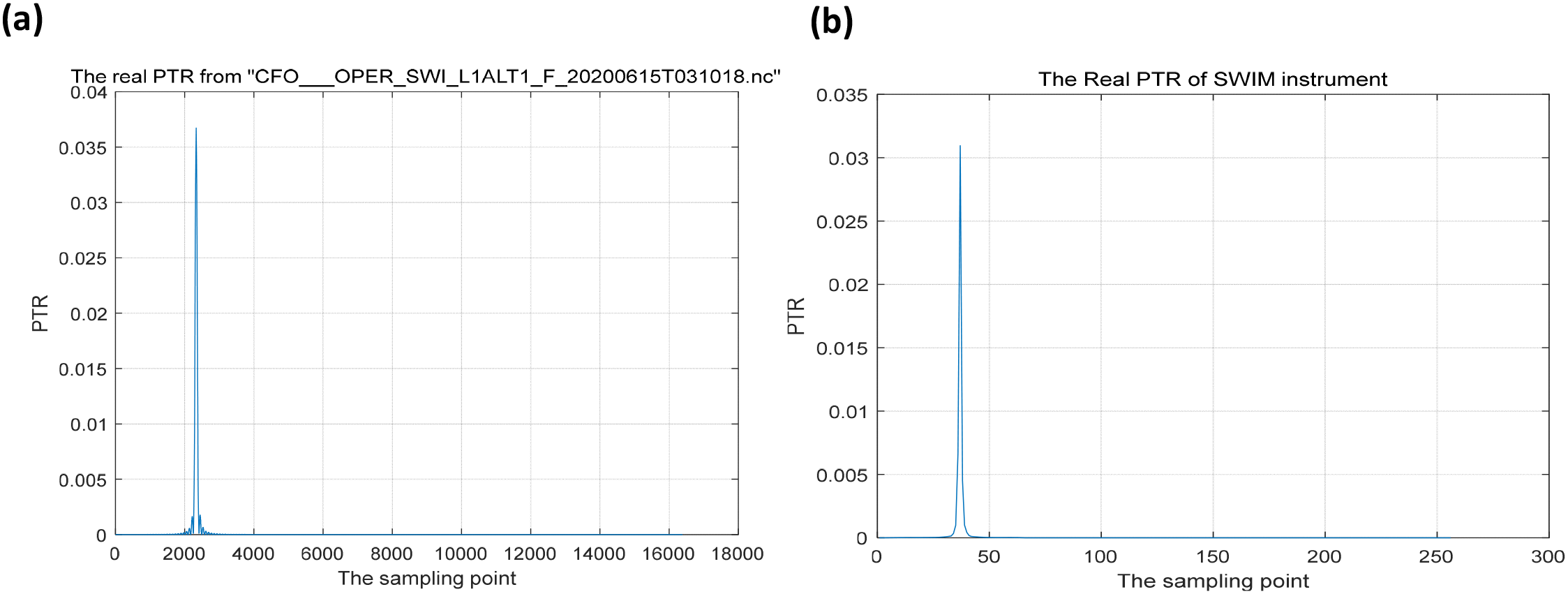
Realistic PTR of the SWIM instrument. (a) Real measurement sample, (b) Mean sample.
In this study, to further enhance the accuracy of inverting SWH by considering the realistic PTR effect, (Equation 10) is used to perform a convolution operation with the real mean PTR of the SWIM instrument (Figure 1b). The improved adaptive algorithm in this article can be given as
where σc = σs and λ' = λs from (Equations 11–20). In MLE6 model, this expression represents an analytical solution after completing a three-term convolution (FSSR*PDF*PTR), which inherently involves operations with the PTR function. However, the current formulation of this (Equation 24) only embodies the analytical result of the first two convolutions (FSSR*PDF), with the second-stage convolution—specifically the convolution with PTR—remaining unperformed. Consequently, it does not incorporate certain PTR-related parameters, implying that the point target response time σp is set to zero (Tourain et al., 2021). Therefore, in (Equation 24) σc = sqrt(σs2 + σp2)= σs and σp is explicitly set to 0. When the measured PTR follows a Gaussian distribution, this equation can be represented by the MLE6 model. This novel technique is executed through the same iterative method as that of Tourain et al. (Tourain et al., 2021), named the Nelder Mead algorithm (Nelder and Mead, 1965). This is a type of direct search technology according to function comparison and often used for solving non-linear optimization problems where those derivative functions of the expected parameters need not be solved first.
2.5 The relationships among these several models
MLE4, whose PDF and PTR are Gaussian distributions, is a conventional re-tracking algorithm that is still used in altimeter missions now. MLE6, whose PDF is non-Gaussian but PTR is a Gaussian distribution, is different from MLE4. From the perspective of parameter inversion, MLE4 and MLE6 are described as re-tracking methods; essentially, both use the Brown theoretical model, with different model simplifications based on the number of tracking parameters required. Although the Gaussian distribution is an acceptable approximation for the PTR related to the altimeter instrument, it is generally different from that of the realistic PTR of an SRA (Rodríguez, 1988). If the PTR of the MLE6 model is substituted with a realistic PTR, MLE6 will further improve its performance in inverting ocean parameters, for example SWH, because it takes into account the real and nonlinear(non-gaussian) random rough sea surface.
To apply realistic PTR, MLE6 is improved into (Equation 24), which is known as the improved adaptive algorithm, where the Gaussian distribution PTR is replaced by the realistic PTR function shown in Figure 1b, which is measured by SWIM, and the PTR of CONV_NONL is replaced by the realistic PTR, which is called CONV_NONL_REAL. The relationships among MLE4, MLE6, and the improved adaptive model are shown in Figure 2.
Figure 2
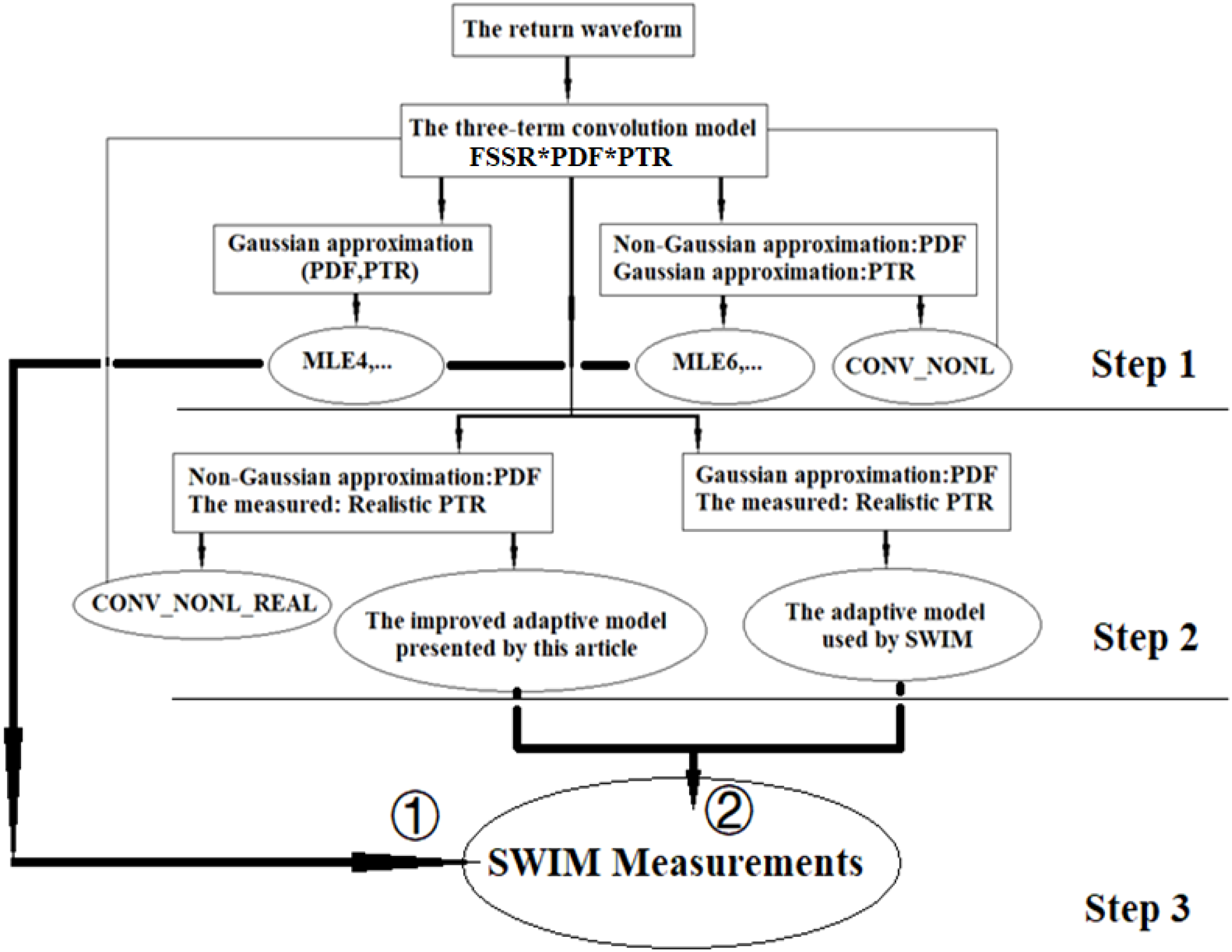
Relationships among several models and flowchart.
In Figure 2, the return waveform is defined by the three-term convolution model(Brown model=FSSR*PDF*PTR). When PDF and PTR are approximated by Gaussian distribution, Brown model is approximated and simplified into the MLE4 model, which is an analytical model. It is simple, has a small computation time, and its accuracy basically meets engineering requirements. However, it only considers the case of a linear(Gaussian) rough sea surface(PDF) and its PTR function of the altimeter is also a Gaussian approximation. In general, the rough random sea surfaces exhibit non-Gaussian distributions, meaning their probability density function (PDF) is non-Gaussian (the polynomial expansion includes skewness and electromagnetic deviation terms). So when PDF is non-gaussian(non-linear) and PTR is gaussian, The Brown model is approximated and simplified into the MLE6 model, which is also an analytical model. Analytical models do not involve convolution operations, resulting in less computation time, simplicity, and high efficiency. Moreover, the point target response (PTR) of a radar is not a Gaussian distribution (Rodríguez, 1988). The PTR of a radar instrument is inherently linked to the instrument’s performance and characteristics. As time progresses and the instrument ages with a shortened service life, the PTR evolves correspondingly (Rodríguez, 1988). When feasible, PTR should be obtained through practical measurements (Tourain et al., 2021). In this context, as the instrument’s operational lifespan extends over time, real-time measurement of its actual PTR and subsequent update of the re-tracking model define an adaptive algorithm or model employed by SWIM (Tourain et al., 2021). However, the existing adaptive model (Tourain et al., 2021) remains a first-order approximation (analogous to MLE3) (Amarouche et al., 2004), with its probability density function (PDF) still assuming a Gaussian distribution. By contrast, the improved adaptive algorithm model proposed in this study is a second-order approximation, similar to MLE4, featuring a non-Gaussian PDF and adaptive PTR updates based on instrument measurements. The PTR function in (Equation 24) will be adaptively updated according to real-time measured values.
In this article, some works will be arranged according to the following steps. Step 1: using the waveforms simulated by the three-term convolution model(Brown model or CONV_NONL) as the true echoes, conduct waveform validation and SWH inversion performance of MLE6 when compared with MLE4. The result will confirm that considering nonlinear (non-gaussian) random ocean surfaces is beneficial for improving SWH inversion accuracy. Step 2: Taking the simulated waveforms by the three-term convolution model (CONV_NONL_REAL, the realistic PTR) as real echoes, complete waveform validation and parameter characteristic analysis of the improved adaptive model by comparing it with the MLE6 model. The compared results will illustrate that accounting for the realistic PTR will enhance the SWH inversion accuracy. Step 3: (1) firstly, use SWIM measurement data to verify that the MLE6 model’s SWH inversion accuracy is superior to MLE4, confirming that considering nonlinear effects of the rough sea surfaces enhances SWH inversion accuracy. (2) Secondly, using the same SWIM waveform data, compare with the adaptive model to validate the improved adaptive model’s enhanced SWH inversion accuracy, also confirming the benefit of nonlinear effect consideration. Compared with step (1), step (2) additionally accounts for adaptive updates of the instrument point target response (PTR) function, further improving SWH inversion accuracy. These steps can be read from the flowchart in Figure 2.
3 SWIM data
On 29 October 2018, the CFOSAT was launched successfully, equipped with a SWIM instrument operated as a Ku-band (13.575GHz) radar with six near-nadir scanning beams at 0°, 2°, 4°, 6°, 8°, and 10° incidence angles. In addition to measuring the directional spectral behaviors of ocean surface waves using off-nadir beams pointed at 6°, 8°, and 10° incidence, SWIM provides nadir products such as SWH, wind speed, and backscattering coefficient σ° etc. at 0° incidence. SWIM can provide a high-accuracy inversion of SWH comparable to traditional altimeter missions by using an adaptive retracking model with a realistic PTR. The European Center Wave Model from the European Centre Medium Weather Forecast (ECMWF) and products from Jason-3 and AltiKa altimeters are the primary references for wind speed and SWH products at 0° incidence. SWIM, when compared to Jason-3 altimeter (Poseidon-3B), showed positive instrumental behavior with adaptive retracking or tracking at the nadir. The adaptive retracking or tracking mode demonstrated similar performance to conventional altimeters over ocean surfaces, with less than 10% error in SWH inversion.
To further explore the performance of MLE6 and its applications, return waveforms from SWIM are selected and processed. In this study, four SWIM tracks in August 2020 and March 2022 are selected, which are termed tracks No. 1, No. 2, No. 3, and No. 4, respectively. In Figure 3, these four tracks are shown, where the red curves represent the running trajectories of SWIM (https://aviso-data-center.cnes.fr/). For track No.1, it may start from point A and end at point B, as shown in Figure 3a. For other tracks, the same logic applies, resulting in a complete track, as shown in Figures 3b–d.
Figure 3
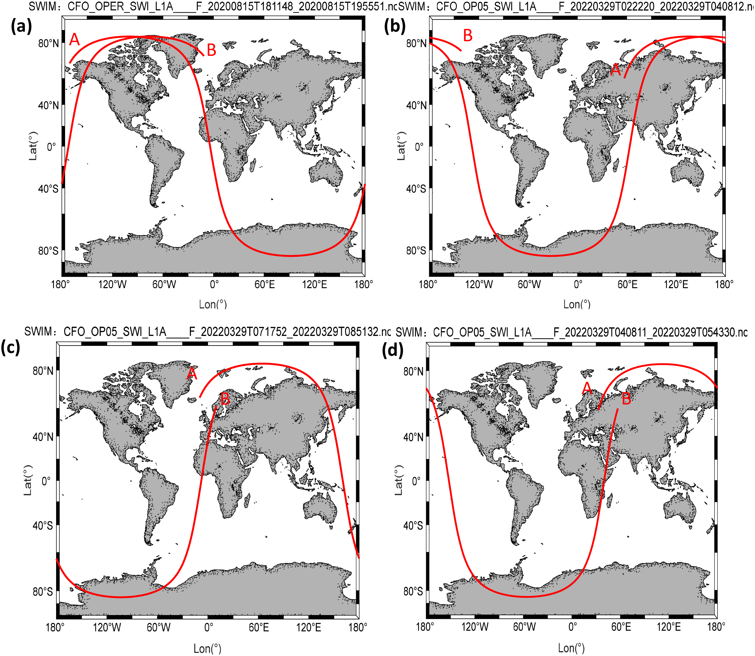
Several SWIM tracks in August 2020 and March 2022. (a) Track No. 1, (b) Track No. 2, (c) Track No. 3, (d) Track No. 4.
4 Results and discussion
4.1 MLE6 validation and SWH inversion
4.1.1 MLE6 waveform validation
Almost no altimeters use the CONV_NONL model to retrack or track the echo waveforms from the rough ocean surface to invert SWH and other ocean parameters. This is because it takes a large amount of time to perform the convolution operations. To invert effectively ocean parameters, the CONV_NONL model is simplified approximately into MLE4 by applying I0(βt1/2)≈2exp(β2t/8)−1 and λs = λem = 0, with PTR and PDF being Gaussian functions. It is simplified approximately into MLE6 by applying I0(βt1/2)≈ 2exp(β2t/8)-1, λs ≠0 and λem ≠0, where PTR is the Gaussian function expressed by (Equation 7), but PDF is the non-Gaussian distribution given by (Equation 8).
In terms of (Equations 15, 20), λem only moves the echo waveform by λemσs/2 along the timeline, but it does not impair the slope of the leading edge of the echo from the random rough ocean surface, and thus it will not impact the accuracy of SWH inversion. Therefore, λem will not be discussed in this article (let λem = 0).
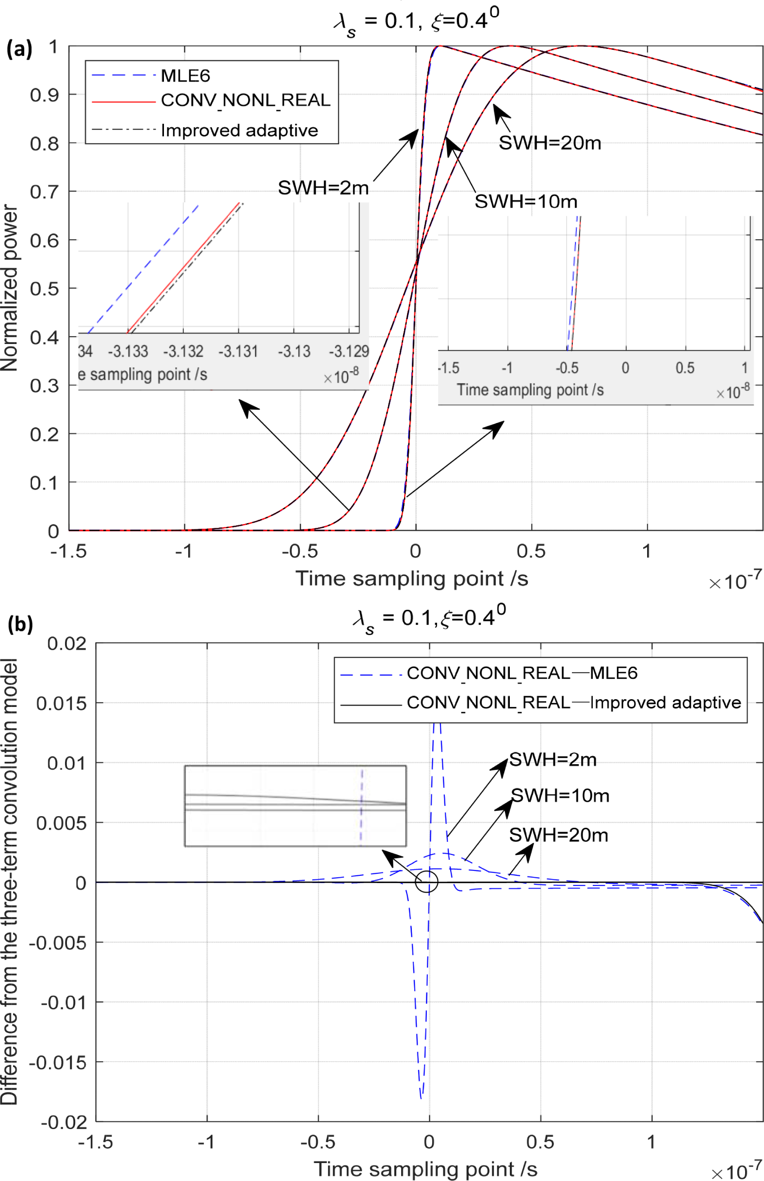
The differences and relationships among CONV_NONL, MLE6, and MLE4 are examined at SWH = 1, 8, 12, 18 m covering low/medium/high sea states, where mispointing angle ξ = 0.4°, non-Gaussian distribution λs = 0.1, and satellite attitude h = 960 km. The echoes simulated by MLE6, MLE4, and CONV_NONL are displayed in Figure 4a. MLE6 is shown to be closer to CONV_NONL than MLE4 under the same conditions and parameters, as depicted in Figure 4a and its subfigures. In Figure 4b, the received normalized power differences between CONV_NONL and MLE6/MLE4 are presented. The differences between CONV_NONL and MLE6 (CONV_NONL-MLE6) represented by solid lines are significantly smaller than those between CONV_NONL and MLE4 (CONV_NONL-MLE4) indicated by dashed lines under sea states (SWH = 1, 8, 12, 18 m). The differences between CONV_NONL (λs = 0.1) and MLE4 (λs = 0) are slightly larger, aligning with Hayne’s (1980) findings, especially observed in the leading edges of the return waveforms. This suggests that MLE4’s accuracy in inverting SWH may be impacted due to the shape or slope of the leading edge of the echo waveform. However, the differences between CONV_NONL and MLE6 are almost negligible, indicating the nearly identical nature of MLE6 to CONV_NONL. This highlights MLE6’s greater efficacy in improving SWH inversion accuracy compared to MLE4. The tail edges of these waveforms are nearly parallel, supported by the retrieved mispointing angles ξ (which are almost identical at 0.4°). If let
Figure 4
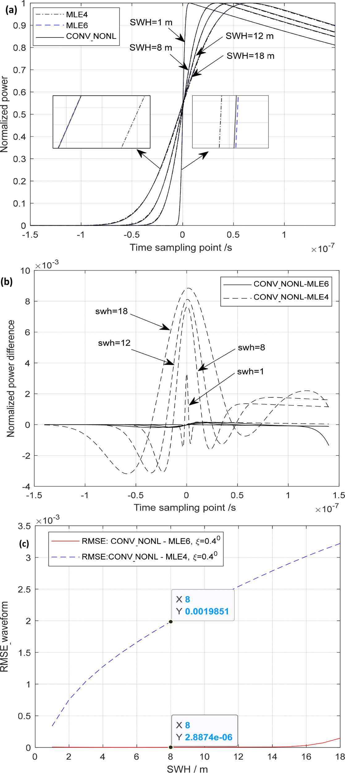
MLE6 and CONV_NONL/MLE4. (a) Comparison between MLE6/MLE4 and CONV_NONL, (b) Differences (CONV_NONL -MLE6) and (CONV_NONL-MLE4), (c) RMSE_waveform of CONV_NONL-MLE6/MLE4.
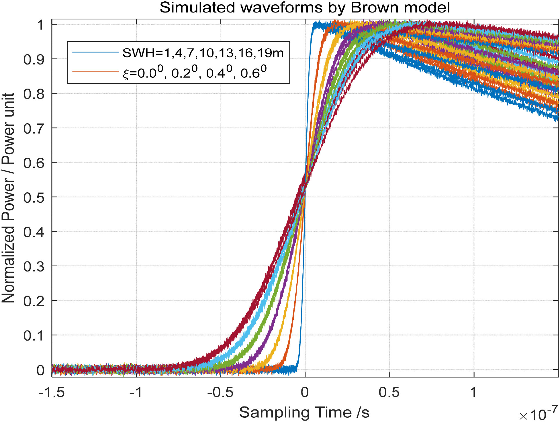
where ti is the time-sampling point. RMSE_waveform (Equation 25) of CONV_NONL-MLE6 (~10−6(normalized unit)) was significantly smaller than that of CONV_NONL-MLE4(~10−3(normalized unit)), as shown in Figure 4c, where ξ = 0.4°. Similarly, the RMSE_waveform of CONV_NONL-MLE6 is smaller than that of CONV_NONL-MLE4 at ξ = 0.2° and 0.6°. MLE6 can more effectively replace the three-term convolution model CONV_NONL to inverse ocean parameters, for example, SWH, from the SRA measurements compared with MLE4.Echo waveforms from random rough ocean surfaces can be simulated by using the three-term convolution model provided by Brown’s model (Brown, 1977), namely, (Equation 1), which is the most accurate expression for ocean echoes among those models. In this section, the echoes simulated by (Equation 1) accounting for non-Gaussian ocean surfaces will be considered to be “the real echoes” to investigate the performance of MLE6 in inverting SWH and other parameters such as skewness coefficient λs.
Assuming the satellite altitude h = 960 km, the beam width is 1.6°, ξ = 0°, 0.2°, 0.4°, 0.6°, and SWH = 1, 2, 3, …, 20 m are possible situations where Gaussian noise is added to echo waveforms. Those simulated waveforms are shown in Figure 5, where λs = 0.1 and 80 simulated waveforms are plotted. We inverted SWH from these 80 waveforms using MLE4 and MLE6. However, the inverted SWH for a return waveform sample is often different from another owing to random Gaussian noise. Therefore, 20 sampling waveforms that can represent a type of sea state with the similar SWH and mispointing angle ξ, are simulated and retracked. The first column in Table 1 represents the true values of SWH and the other two columns represent the values inverted by MLE6 and MLE4, respectively. The accuracy of estimating SWH using MLE6 is better than that using MLE4, which can be demonstrated by calculating the root mean square error (RMSE) and Mean Bias as follows:
Figure 5
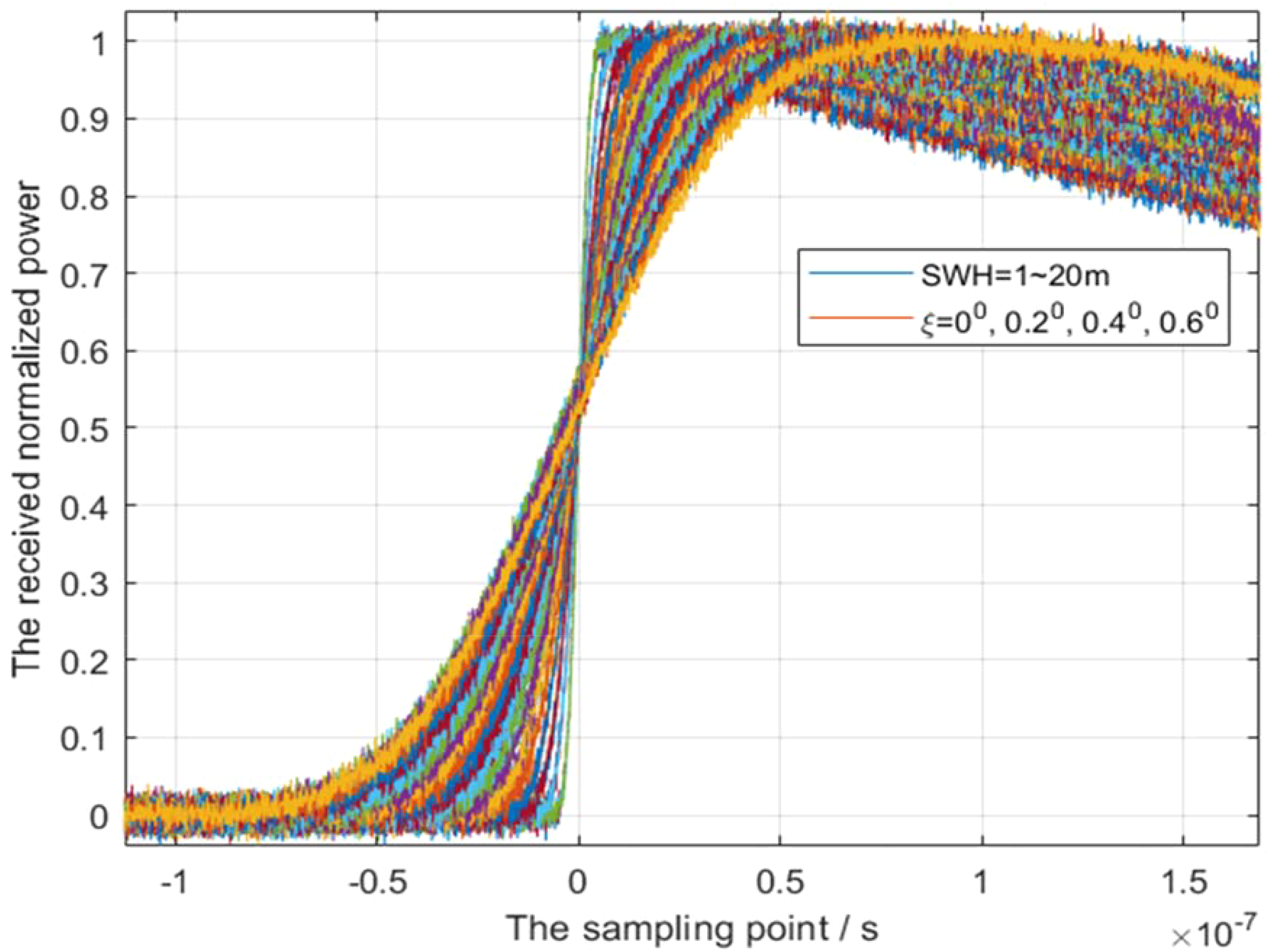
Simulated echoes by three-term convolution model CONV_NONL.
Table 1
| ξ SWH/m | 0.00 MLE4 | 0.00 MLE6 | 0.20 MLE4 | 0.20 MLE6 | 0.40 MLE4 | 0.40 MLE6 | 0.60 MLE4 | 0.60 MLE6 |
|---|---|---|---|---|---|---|---|---|
| 1 | 1.003 | 1.002 | 0.996 | 0.996 | 0.988 | 0.988 | 1.001 | 1.000 |
| 2 | 1.989 | 1.990 | 1.996 | 1.996 | 2.005 | 2.003 | 1.986 | 1.987 |
| 3 | 2.979 | 2.982 | 2.986 | 2.988 | 3.008 | 3.006 | 2.975 | 2.979 |
| 4 | 4.006 | 4.004 | 3.989 | 3.994 | 3.968 | 3.976 | 4.000 | 3.999 |
| 5 | 4.962 | 4.973 | 4.985 | 4.989 | 4.996 | 4.996 | 4.954 | 4.968 |
| 6 | 5.985 | 5.990 | 5.976 | 5.984 | 5.997 | 5.998 | 5.977 | 5.986 |
| 7 | 6.980 | 6.987 | 6.958 | 6.977 | 6.981 | 6.991 | 6.962 | 6.974 |
| 8 | 7.975 | 7.990 | 7.966 | 7.988 | 7.963 | 7.984 | 7.958 | 7.982 |
| 9 | 8.976 | 8.992 | 8.937 | 8.983 | 8.948 | 8.988 | 8.946 | 8.984 |
| 10 | 9.952 | 9.989 | 9.937 | 9.977 | 9.910 | 9.964 | 9.918 | 9.975 |
| 11 | 10.986 | 11.000 | 10.953 | 10.996 | 10.904 | 10.977 | 10.932 | 10.994 |
| 12 | 11.964 | 12.000 | 11.931 | 11.991 | 11.927 | 11.979 | 11.920 | 11.995 |
| 13 | 12.985 | 13.000 | 12.916 | 12.987 | 12.901 | 12.988 | 12.910 | 12.992 |
| 14 | 13.999 | 13.999 | 13.884 | 13.991 | 13.884 | 13.994 | 13.924 | 14.000 |
| 15 | 14.974 | 14.999 | 14.892 | 14.992 | 14.896 | 14.999 | 14.858 | 14.997 |
| 16 | 15.974 | 15.998 | 15.870 | 16.000 | 15.880 | 15.999 | 15.940 | 16.000 |
| 17 | 16.992 | 16.999 | 16.907 | 16.997 | 16.904 | 17.000 | 16.971 | 17.000 |
| 18 | 18.001 | 17.998 | 17.917 | 18.000 | 17.931 | 18.000 | 17.957 | 18.000 |
| 19 | 19.038 | 18.997 | 18.963 | 19.000 | 19.061 | 19.000 | 19.078 | 19.000 |
| 20 | 19.984 | 19.997 | 19.974 | 20.000 | 20.046 | 19.999 | 20.091 | 20.004 |
| RMSE | 0.070 | 0.022 | 0.094 | 0.028 | 0.102 | 0.030 | 0.100 | 0.0280 |
| MeanBias | 0.043 | 0.011 | 0.080 | 0.015 | 0.082 | 0.015 | 0.081 | 0.012 |
Estimated SWH by applying MLE6 (λs = 0.1) and MLE4.
where SWHitru represents the true value of SWH, SWHiest represents the values estimated by the MLE4 or MLE6 algorithm. By inverting and calculating at ξ = 0.0°, 0.2°, 0.4°, and 0.6°, the Mean Bias (Equation 26) of SWH estimated by MLE6 are less than those estimated by MLE4, as is the RMSE (Equation 27), as listed in the 21st and 22nd rows in Table 1.
In Table 1, the estimated SWHs represent the mean values of 20 samples. For example, at ξ = 0.0° and SWH = 1 m, 1.0021 m is the mean value of the estimated SWH by MLE6 over 20 various simulated waveforms to which random Gaussian noises are added. Figure 6 shows the estimated SWH at ξ = 0.0° 20 samples, where Mean Biases of the estimated SWH by applying MLE6, varying from 0.45 cm to 2.03 cm (mean value = 1.11 cm listed (Table 1), were smaller than those estimated by MLE4, varying from 2.54 cm to 8.79 cm (mean value = 4.33 cm listed (Table 1). The mean improvement was 3.23 cm, as indicated by the green dotted line in Figure 6a. In Figure 6b, RMSEs of the estimated SWHs by applying MLE6, varying from 0.86 cm to 4.36 cm (mean value = 2.24 cm listed in Table 1), were smaller than those estimated by MLE4, varying from 3.81 cm to 15.06 cm (mean value = 6.98 cm listed in Table 1). The mean improved amount is 4.74 cm, as shown by the green dot line in Figure 6b.
Figure 6
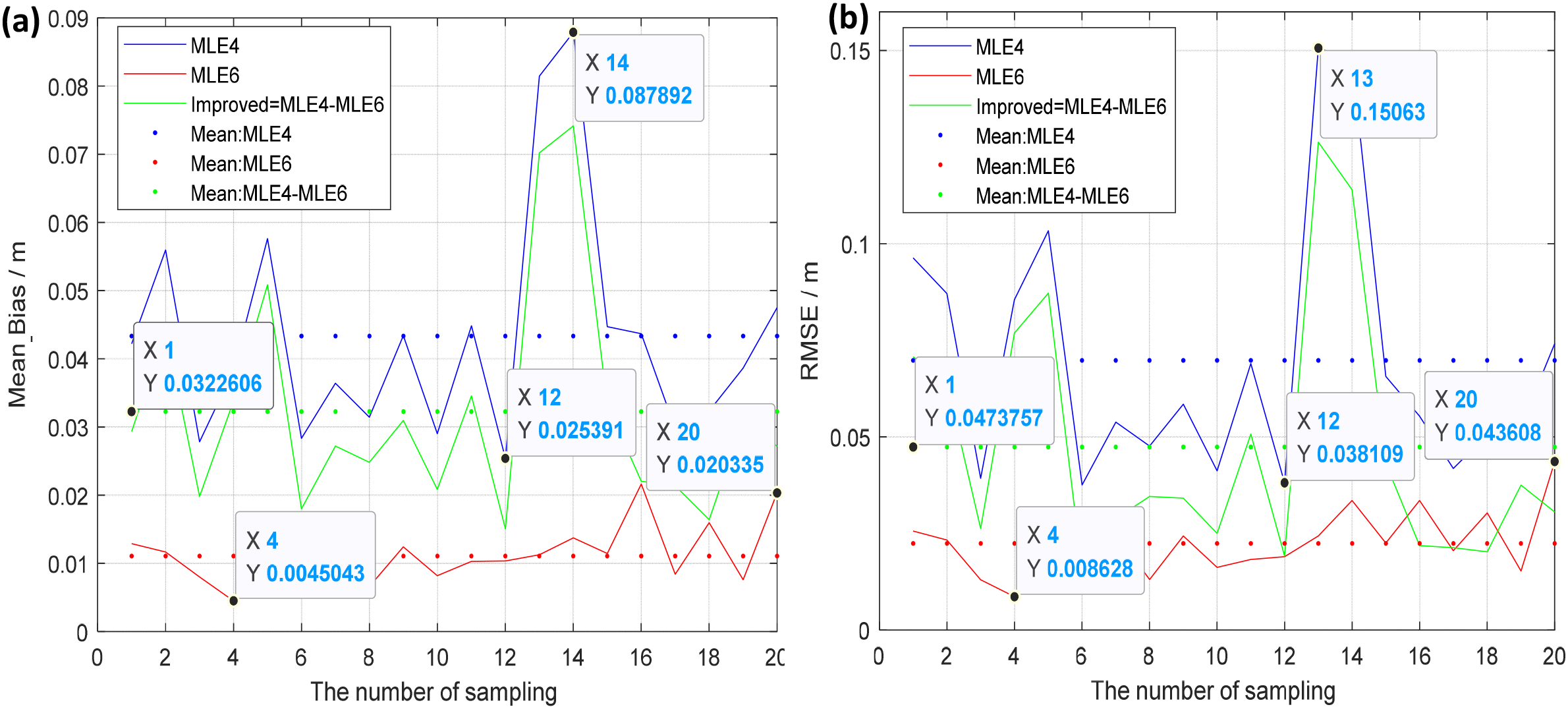
Mean Bias/RMSE varying with various samples. (a) Mean Bias at ξ = 0.0°, (b) RMSE at ξ = 0.0°.
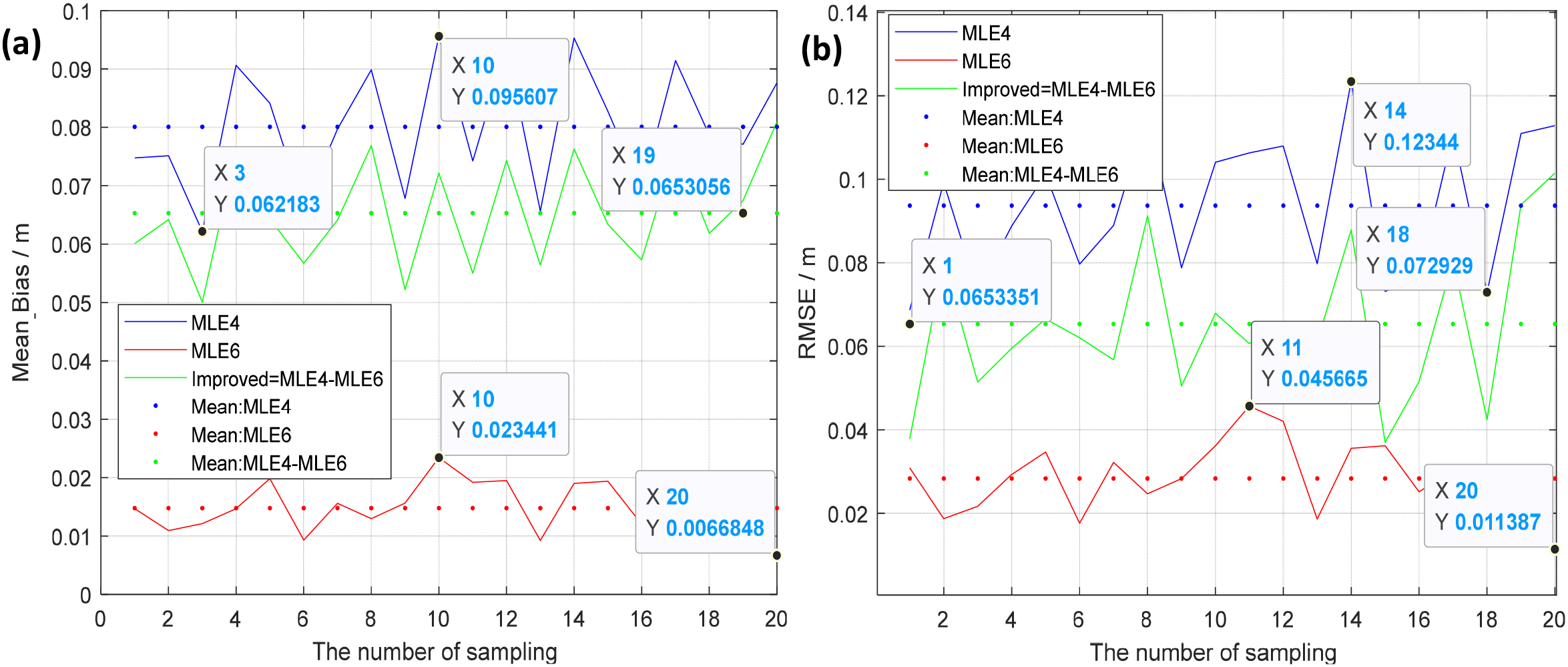
Figure 7 shows the estimated SWH at ξ = 0.2° 20 samples, where Mean Biases of the estimated SWH by applying MLE6, varying from 0.67 cm to 2.34 cm (mean value = 1.48 cm listed in Table 1), were substantially smaller than those estimated by MLE4, varying from 6.22 cm to 9.56 cm (mean value = 8.01 cm listed (Table 1). The mean improvement amount is 6.53 cm, as shown by the green dotted line in Figure 7a. Figure 7b shows RMSEs of the estimated SWHs by applying MLE6 and MLE4, respectively. Here, the RMSEs of the estimated SWHs by applying MLE6, varying from 1.14 cm to 4.57 cm (mean value = 2.83 cm listed in Table 1), were substantially smaller than those by MLE4, varying from 7.29 cm to 12.34 cm (mean value = 9.37 cm list in Table 1). The mean improved amount is 6.53 cm, as shown by the green dot line. Figure 8 shows the estimated SWH at ξ = 0.4° 20 samples, where the Mean Biases of the estimated SWHs by applying MLE6, varying from 0.67 cm to 2.48 cm (mean value = 1.50 cm listed in Table 1), were much smaller than those obtained by MLE4, varying from 5.60 cm to 11.65 cm (mean value = 8.22 cm listed (Table 1). The mean improvement was 6.72 cm, as indicated by the green dotted line in Figure 8a. In Figure 8b, RMSEs of the estimated SWHs by applying MLE6, varying from 1.52 cm to 5.75 cm (mean value=2.95 cm listed in Table 1), were substantially smaller than those by MLE4, varying from 7.13 cm to 12.40 cm (mean value = 10.15 cm listed in Table 1). The mean improvement in the estimated SWH was 7.20 cm, as indicated by the green dotted line.
Figure 7
Mean Bias/RMSE varies with various samples. (a) Mean Bias at ξ = 0.2°, (b) RMSE at ξ = 0.2°.
Figure 8
Mean Bias/RMSE varying with various samples. (a) Mean Bias at ξ = 0.4°, (b) RMSE at ξ = 0.4°.
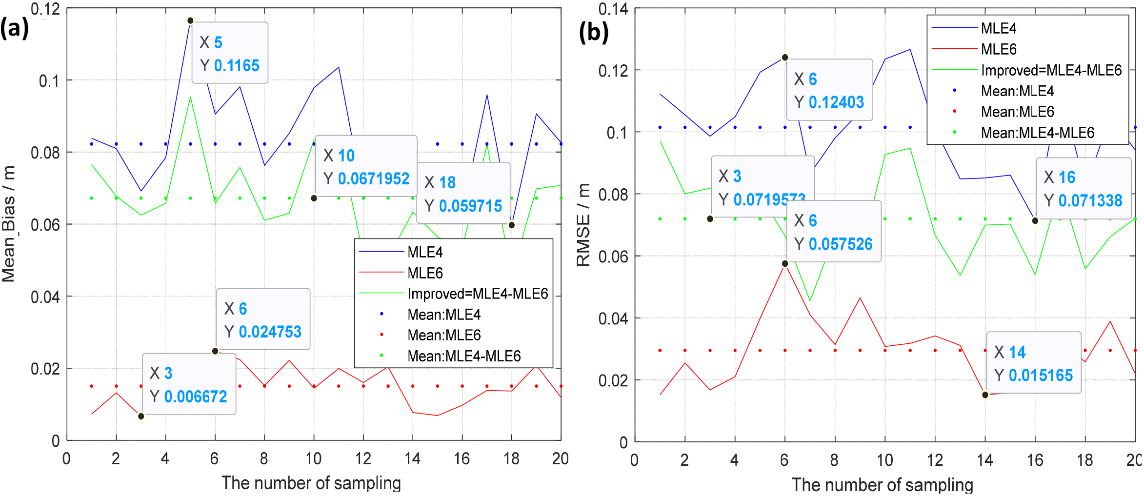
Figure 9 shows the estimated SWH at ξ = 0.6° 20 samples, where Mean Biases of the estimated SWHs by MLE6, varying from 0.86 cm to 2.82 cm (mean value = 1.47 cm listed in Table 1), were substantially smaller than those by MLE4, varying from 5.75 cm to 11.03 cm (mean value = 8.06 cm listed in Table 1). The mean improvement in the estimated SWH is 6.58 cm, as indicated by the green dotted line in Figure 9a. Figure 9b shows RMSEs of the estimated SWHs by applying MLE6 and MLE4, respectively; RMSEs of the estimated SWHs by MLE6, varying from 1.48 cm to 4.03 cm (mean value = 2.83 cm listed in Table 1), were substantially smaller than those by MLE4, varying from 7.02 cm to 16.24 cm (mean value= 9.97 cm list in Table 1). The mean improvement in the estimated SWH was 7.14 cm, as indicated by the green dotted line.
Figure 9
Mean Bias/RMSE varying with various samples. (a) Mean Bias at ξ = 0.6°, (b) RMSE at ξ = 0.6°.
From Figures 6–9 and Table 1, some conclusions can be obtained: (1) Mean Bias and RMSE of the estimated SWHs by MLE6 (1.11, 1.48, 1.50, 1.47 cm; 2.24, 2.83, 2.95, 2.83 cm), from approximately 1 to 3 cm, were smaller than those by estimated MLE4 (4.33, 8.01, 8.22, 8.06 cm; 6.98, 9.37, 10.15, 9.97 cm), from approximately 4 to 10 cm. This demonstrates that the accuracy of estimating SWH can be enhanced by the amount from 4.74 to 7.2 cm in RMSE, from 3.22 cm to 6.72 cm in Mean Bias by applying MLE6 with accounting for non-Gaussian effects. The mean total improvement was approximately 3.1630 cm. (2) The amount of improvement increases with the mispointing angle ξ increasing, but does not when ξ exceeds 0.4°. The improvement remained almost unchanged when ξ >0.4°. (3) The fluctuation amplitudes of RMSE and Mean Bias of the estimated SWH by MLE6 were much smaller than those estimated by MLE4, as shown by the red and blue solid lines in Figures 6–9. The accuracy of inverting SWH using MLE6 was relatively stable and higher than that of MLE4.
4.1.2 Skewness coefficient retrieval from the simulated waveforms
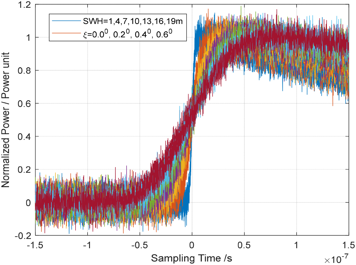
Similarly, assuming the satellite altitude h = 960 km, the beam width is 1.6°, ξ = 0°, 0.2°, 0.4°, 0.6°, and SWH = 1, 4, 7, …, 19 m are possible situations where Gaussian noise is added to echo waveforms. In Figure 10, the simulated waveforms is simulated by Brown model with λs=0.1 and λem=0.0, where waveforms with λs=0.2 and λem=0.0 are not shown.
Figure 10
The simulated waveforms by Brown model with λs=0.1 and λem=0.
To evaluate the performance of MLE6 in inverting the skewness coefficient, both the Brown model and MLE6 were used to track these waveforms simultaneously. The re-tracking results are shown in Table 2. From Table 2, the performance of MLE6 model in inverting parameter λs is almost identical to that of the Brown model. The inversion bias ranges of the two models are between 0.005 and 0.012 (<12%), and the specific error magnitude depends on the noise level(eg. signal/noise=1:0.01), with little relationship to SWH and mispointing angle ξ. If the noise is not added to these simulated waveforms, the retrieved λs is almost identical to the real values by using MLE6 and Brown model.
Table 2
| Mispointing angle/0 | SWH/m | Real λs | λs by MLE6 | λs by Brown model | Real λs | λs by MLE6 | λs by Brown model |
|---|---|---|---|---|---|---|---|
| 0 | 1 | 0.1 | 0.122 | 0.122 | 0.2 | 0.182 | 0.182 |
| 0 | 4 | 0.1 | 0.090 | 0.090 | 0.2 | 0.190 | 0.190 |
| 0 | 7 | 0.1 | 0.106 | 0.106 | 0.2 | 0.194 | 0.194 |
| 0 | 10 | 0.1 | 0.100 | 0.100 | 0.2 | 0.204 | 0.206 |
| 0 | 13 | 0.1 | 0.104 | 0.104 | 0.2 | 0.200 | 0.200 |
| 0 | 16 | 0.1 | 0.104 | 0.104 | 0.2 | 0.194 | 0.194 |
| 0 | 19 | 0.1 | 0.094 | 0.096 | 0.2 | 0.196 | 0.198 |
| 0.2 | 1 | 0.1 | 0.096 | 0.096 | 0.2 | 0.194 | 0.194 |
| 0.2 | 4 | 0.1 | 0.098 | 0.098 | 0.2 | 0.208 | 0.208 |
| 0.2 | 7 | 0.1 | 0.110 | 0.110 | 0.2 | 0.194 | 0.194 |
| 0.2 | 10 | 0.1 | 0.102 | 0.102 | 0.2 | 0.200 | 0.200 |
| 0.2 | 13 | 0.1 | 0.098 | 0.098 | 0.2 | 0.202 | 0.202 |
| 0.2 | 16 | 0.1 | 0.100 | 0.100 | 0.2 | 0.202 | 0.204 |
| 0.2 | 19 | 0.1 | 0.094 | 0.096 | 0.2 | 0.198 | 0.200 |
| 0.4 | 1 | 0.1 | 0.102 | 0.102 | 0.2 | 0.184 | 0.184 |
| 0.4 | 4 | 0.1 | 0.108 | 0.108 | 0.2 | 0.194 | 0.194 |
| 0.4 | 7 | 0.1 | 0.098 | 0.098 | 0.2 | 0.198 | 0.198 |
| 0.4 | 10 | 0.1 | 0.098 | 0.098 | 0.2 | 0.200 | 0.200 |
| 0.4 | 13 | 0.1 | 0.096 | 0.096 | 0.2 | 0.192 | 0.194 |
| 0.4 | 16 | 0.1 | 0.104 | 0.104 | 0.2 | 0.198 | 0.198 |
| 0.4 | 19 | 0.1 | 0.100 | 0.100 | 0.2 | 0.196 | 0.198 |
| 0.6 | 1 | 0.1 | 0.080 | 0.080 | 0.2 | 0.202 | 0.204 |
| 0.6 | 4 | 0.1 | 0.104 | 0.104 | 0.2 | 0.200 | 0.200 |
| 0.6 | 7 | 0.1 | 0.104 | 0.104 | 0.2 | 0.206 | 0.208 |
| 0.6 | 10 | 0.1 | 0.098 | 0.098 | 0.2 | 0.204 | 0.204 |
| 0.6 | 13 | 0.1 | 0.104 | 0.104 | 0.2 | 0.194 | 0.194 |
| 0.6 | 16 | 0.1 | 0.100 | 0.102 | 0.2 | 0.204 | 0.204 |
| 0.6 | 19 | 0.1 | 0.096 | 0.098 | 0.2 | 0.200 | 0.202 |
| RMSE | – | – | 0.012 | 0.012 | – | 0.006 | 0.006 |
| Mean value | – | 0.1 | 0.098 | 0.098 | 0.2 | 0.198 | 0.198 |
The retrieved λs by MLE6 and brown model.
For another example, when the added noise is high (simulated waveforms are shown in Figure 11), the retrieved skewness coefficient λs has a large deviation of up to 0.07(RMSE=0.0717, 0.0719 for MLE6, Brown model) and fluctuates significantly, but the average value is still close to 0.1(mean values=0.1139, 0.1148 for MLE6, Brown model), as shown in Figure 12. In Figure 12, the retrieved skewness coefficient λs varies with SWH=1,4,7,10,13,16,19m at mispointing angle ξ=00, 0.20, 0.40, 0.60. the real skewness coefficient λs =0.1. Therefore, minimizing noise interference can greatly reduce the parameter λs inversion error. All in all, the performance of MLE6 in retrieving λs is almost the same as that of Brown model.
Figure 11
The simulated waveform with a large noise.
Figure 12
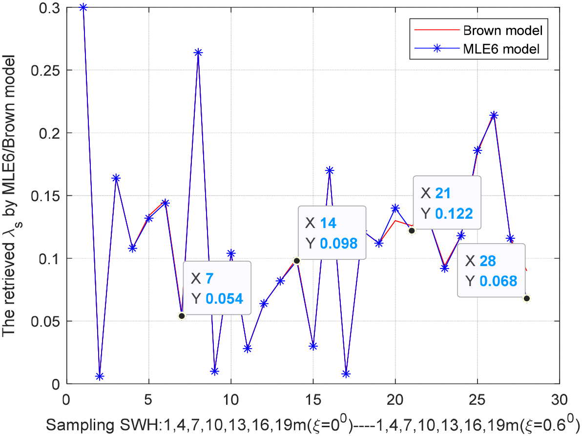
The retrieved λs varying with SWH and ξ.
4.1.3 Electromagnetic bias coefficient λem validation
Electromagnetic (EM) bias coefficient λem is difficult to obtain from re-tracking waveforms (Rodríguez, 1988). because the electromagnetic bias only shifts the waveforms, leading to the later arrival of the half-power point (average energy). Since the crests of the sea surface are more susceptible to wind, their scattering coefficient is lower (because wind speed is negatively correlated with the scattering coefficient). The probability density of the scattering field tends to favor the wave troughs, resulting in the fact that the average height of the scattering points (radar apparent height) is below the average sea surface height. This error is called electromagnetic bias. The mean value of the sea surface scattering field is lower than the mean sea surface height. The effect of the later arrival of the scattering pulse sign is consistent with that of a decrease in sea surface height. It is difficult to distinguish both of them according to the mathematical expressions or (Equations 15, 20).
The electromagnetic bias may be implicit in t0 when re-tracking the echoes. That is to say, if a bias occurs, it is difficult to distinguish whether the bias is due to t0 or λemσs/2 (Rodríguez, 1988). So in this manuscript the electromagnetic bias is not discussed.
However, the accuracy of MLE6 can be analyzed by comparing whether the movement amount of MLE6 is the same as that of Brown model when the electromagnetic bias coefficient λem is given as a series of values shown in Figure 13. It is obvious that the movement amount of MLE6 is the same as that of Brown model, and the electromagnetic bias can be given as (Rodríguez, 1988).
Figure 13
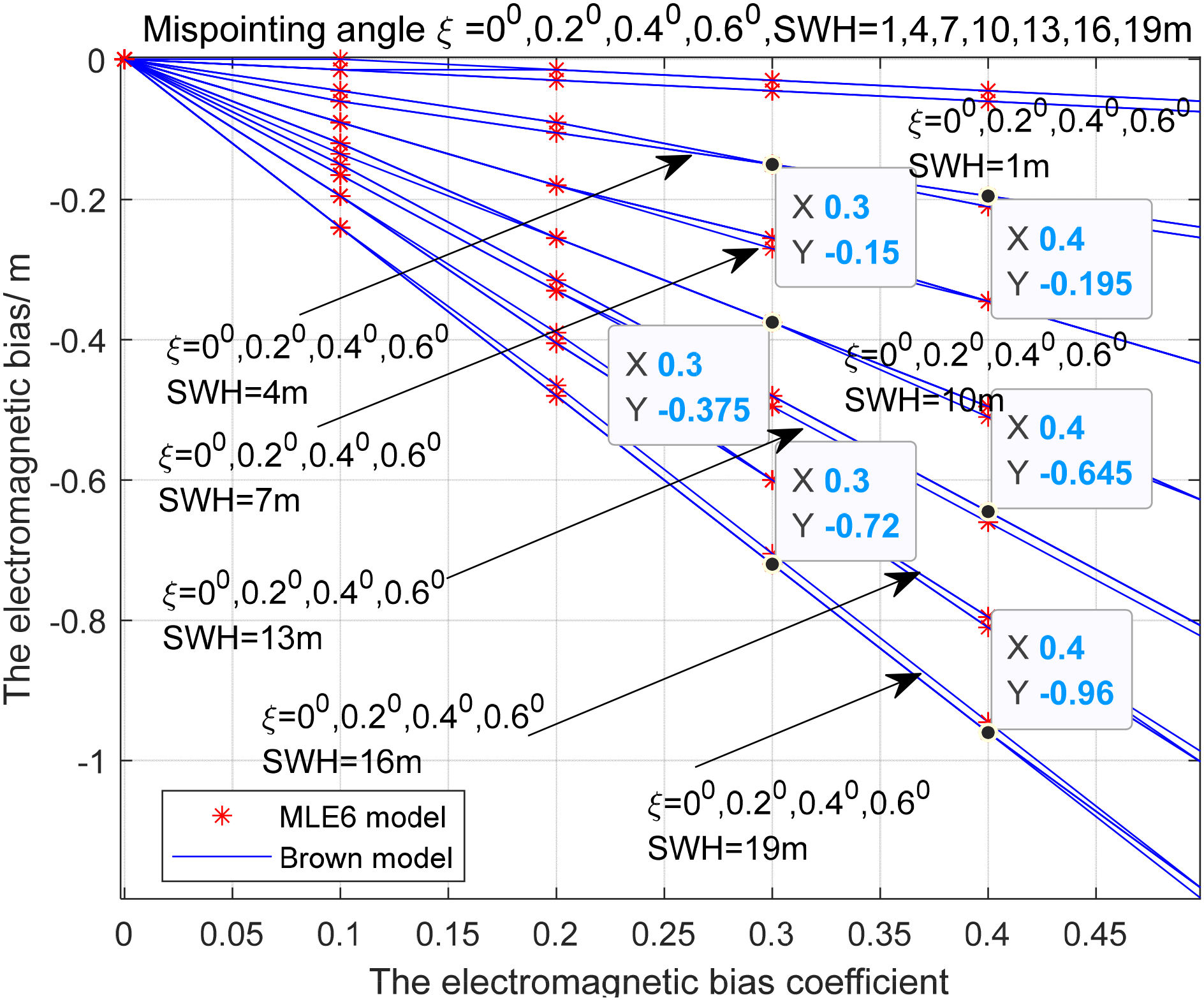
EM bias varying with EM bias coefficient at various SWH and mispointing angle.
based on the data in Figure 13 or Equation 28, EM bias is almost no related to mispointing angle ξ.
All in all, the performance of MLE6 in retrieving parameters such as λs and λem is identical to that of Brown model, but MLE6 has no convolution operations, resulting in small computational load, high efficiency, and easy real-time application on satellites.
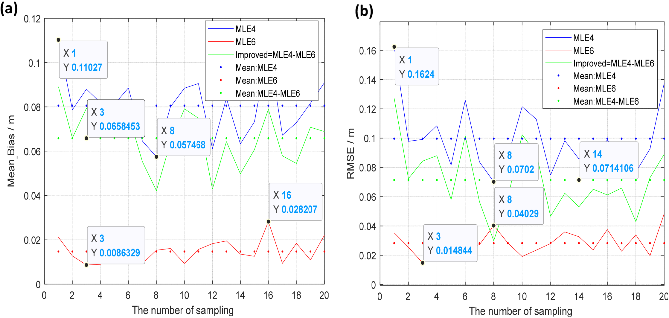
4.2 SWH retrieval from SWIM data by MLE6
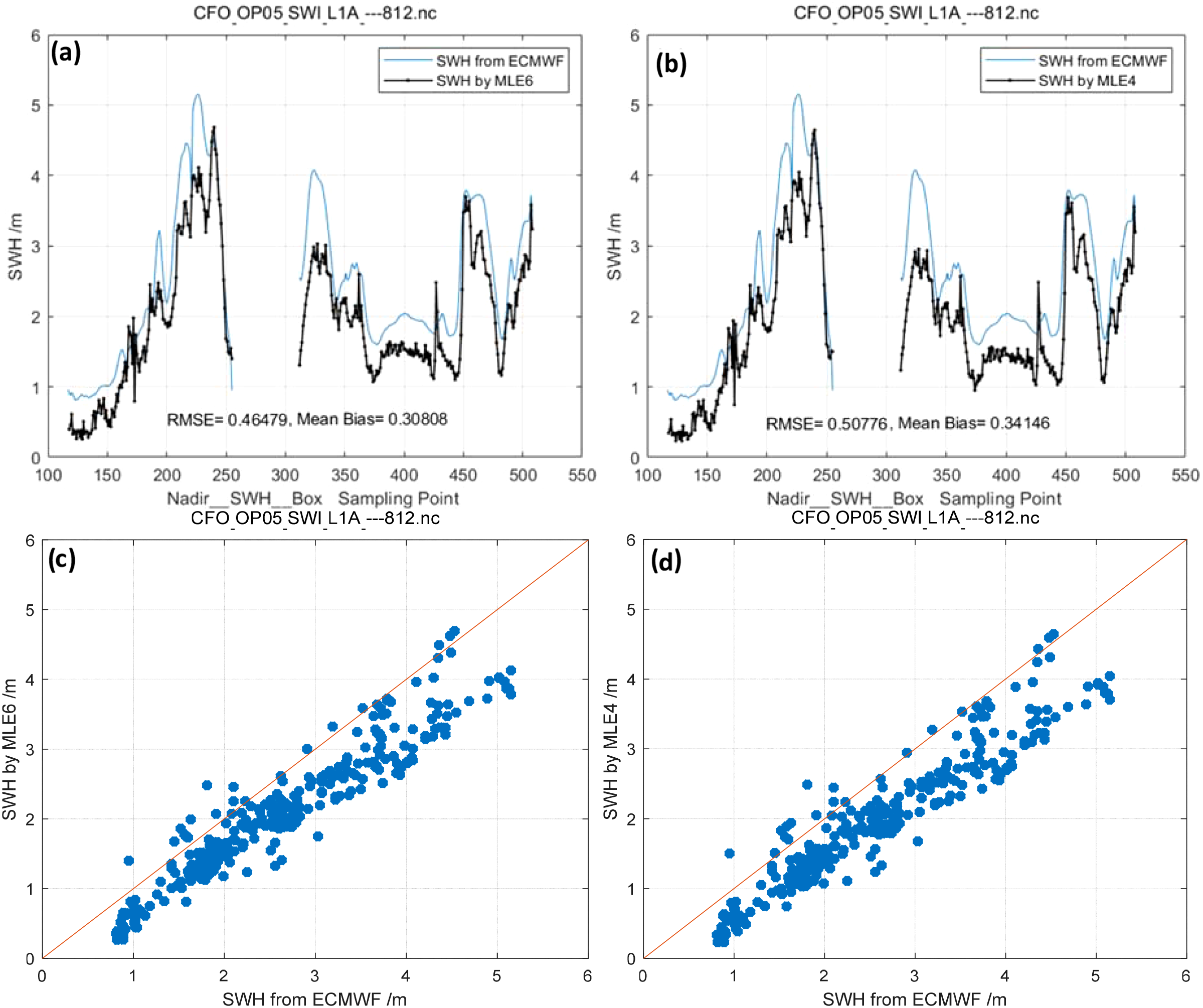
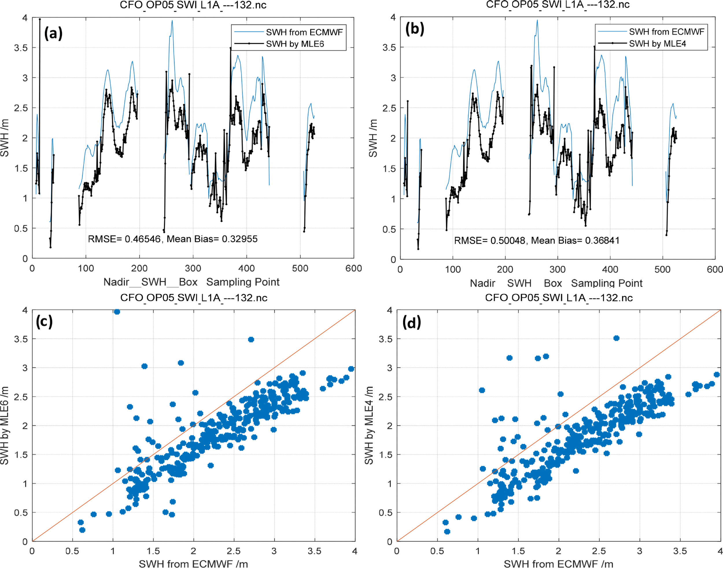
Using SWH products from ECMWF as the reference, we applied both the MLE6 and MLE4 algorithms to invert SWH from SWIM measurements [level 1 A [L1A] (https://aviso-data-center.cnes.fr/)] at 0° incidence. The inverted SWHs, “box average values,” were compared with collocated model data (ECMWF), as depicted in Figures 14–17. Mean Bias and RMSE of the SWH estimated by MLE6 (0.28994, 0.46479, 0.46546, and 0.63556 m) were smaller than those estimated by MLE4 (0.32847, 0.50776, 0.50048, and 0.67728 m). This indicates that considering non-Gaussian height distribution of rough ocean surfaces can improve the accuracy of SWH inversion, which is a 3–4 cm improvement in RMSE of SWH retrieval; additionally, Mean Bias of SWH inversion was improved by 4 cm (0.04297 m denoted by Figure 18b and in Table 3). These results are in line with the simulation results presented in Section 4.1.1.
Figure 14
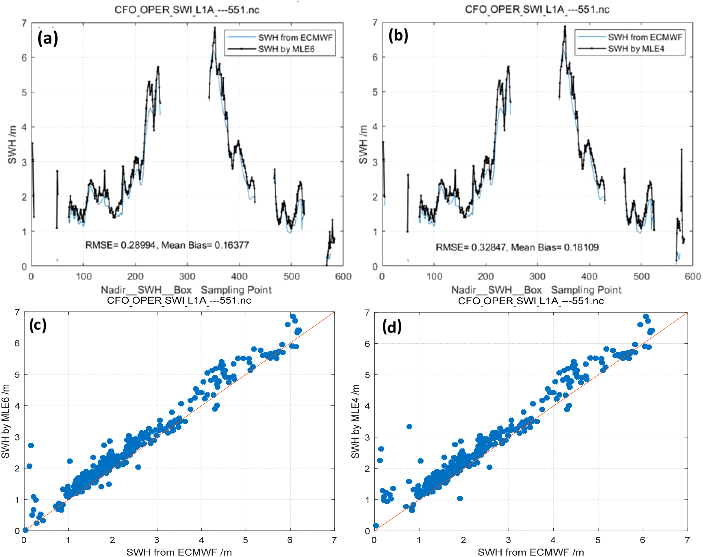
Track No. 1: SWH retrieved by MLE6 (Mean λs = 0.10735)/MLE4 compared with collocated model data (ECMWF). (a) SWH retrieved by MLE6, (b) SWH retrieved by MLE4. (c) Scatter plots for SWH retrieved by MLE6, (d) Scatter plots for SWH retrieved by MLE4.
Figure 15
Track No. 2: SWH retrieved by MLE6 (Mean λs = 0.12932)/MLE4 compared with collocated model data (ECMWF). (a) SWH retrieved by MLE6, (b) SWH retrieved by MLE4. (c) Scatter plots for SWH retrieved by MLE6, (d) Scatter plots for SWH retrieved by MLE4.
Figure 16
Track No. 3: SWH retrieved by MLE6 (Mean λs = 0.12972)/MLE4 compared with collocated model data (ECMWF). (a) SWH retrieved by MLE6, (b) SWH retrieved by MLE4. (c) Scatter plots for SWH retrieved by MLE6, (d) Scatter plots for SWH retrieved by MLE4.
Figure 17
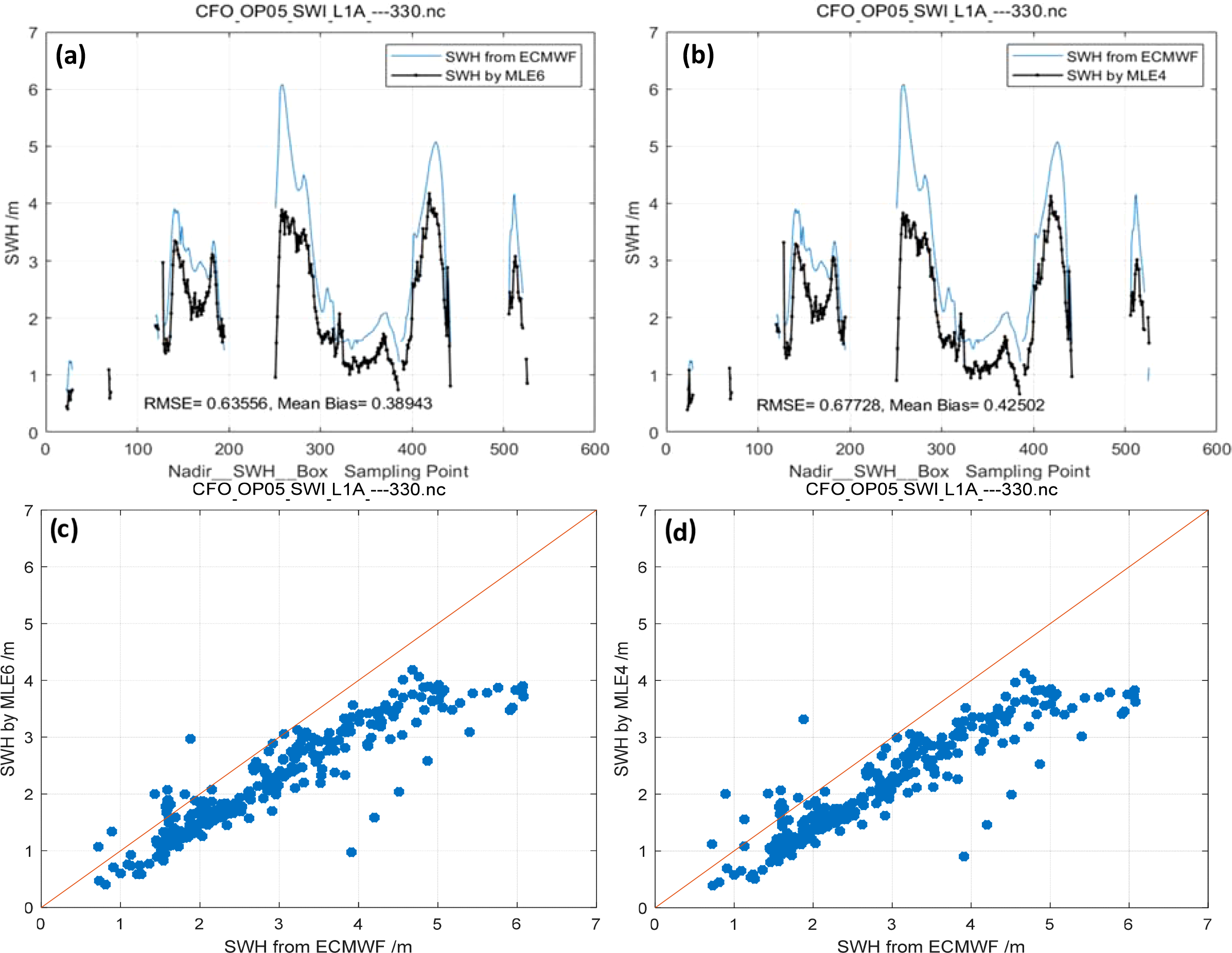
Track No. 4: SWH retrieved by MLE6 (Mean λs = 0.13217)/MLE4 compared with collocated model data (ECMWF). (a) SWH retrieved by MLE6, (b) SWH retrieved by MLE4. (c) Scatter plots for SWH retrieved by MLE6, (d) Scatter plots for SWH retrieved by MLE4.
Figure 18
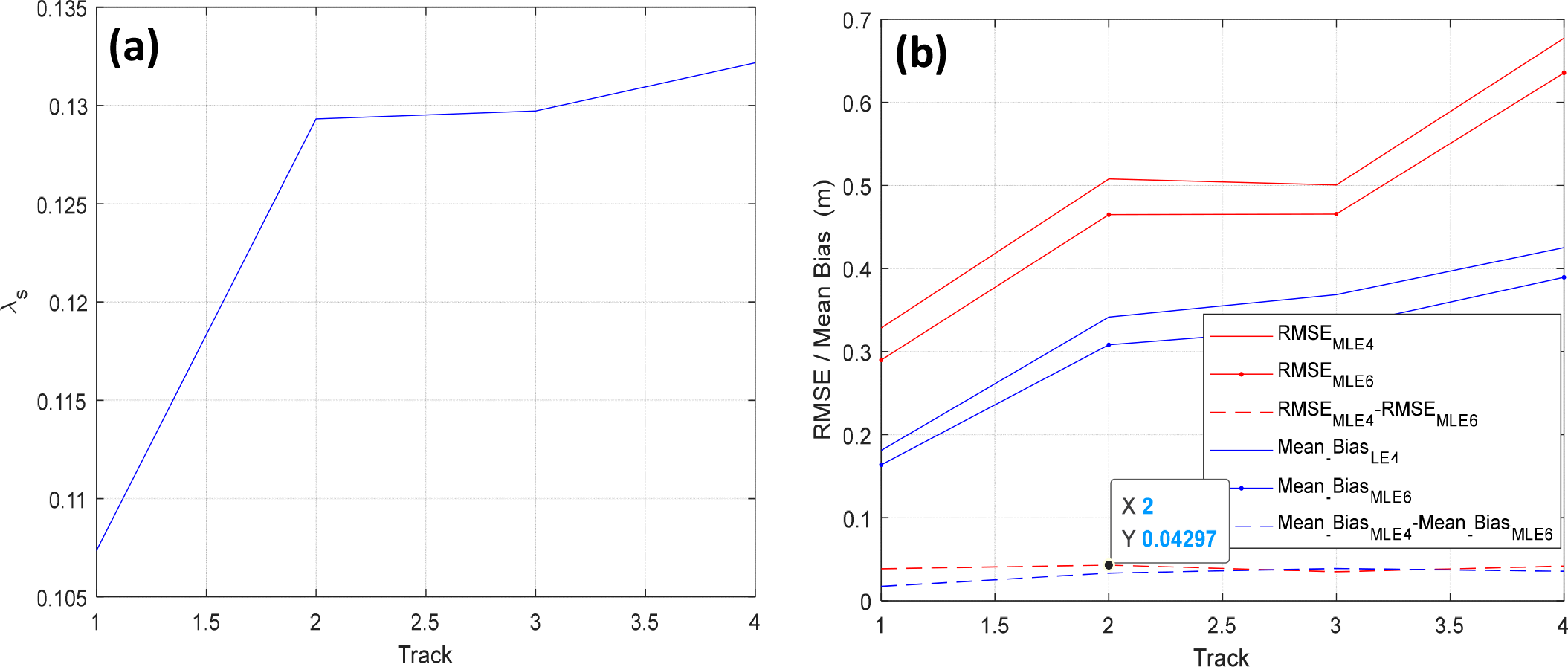
Estimated λs and Mean Bias/RMSE of SWH are estimated by MLE6 and MLE4. (a) The retrieved λs, (b) RMSE/Mean_Bias and their differences.
Table 3
| Track/num | Model | Mean λs | RMSE/m | Mean Bias/m |
|---|---|---|---|---|
| NO.1/18619 | MLE4 | 0 | 0.329 | 0.181 |
| MLE6 | 0.107 | 0.290 | 0.164 | |
| NO.2/17350 | MLE4 | 0 | 0.508 | 0.341 |
| MLE6 | 0.129 | 0.465 | 0.308 | |
| NO.3/17638 | MLE4 | 0 | 0.500 | 0.368 |
| MLE6 | 0.130 | 0.465 | 0.330 | |
| NO.4/15562 | MLE4 | 0 | 0.677 | 0.425 |
| MLE6 | 0.132 | 0.636 | 0.389 |
Deviation of SWH estimated by MLE6 and MLE4 when compared with ECMWF.
Track No. 1 occurred on 15 August 2020. The effects of the non-Gaussian distribution of sea surface elevation are rather weak owing to the small λs, with a mean value of 0.10735 denoted by Figure 18a. Therefore, the improvement of inverting SWH is weaker than others’. Tracks No. 2, No.3 and No.4 occurred on 29 March 2022. The effects of the non-Gaussian distribution of rough sea surfaces were slightly stronger, with a mean value of 0.1304, which is almost consistent with the reported values (Thibaut et al., 2005). The Number of waveforms for No.1 is 18619, No.2 17350, No.3 17638, No.4 15562, as listed in Table 3. From Figures 14–17, box average values are shown. These sampling points or waveforms illustrated that MLE6 was robust in a considerable degree. Moreover, some scatter plots are given, as can be seen from Figures 13–17C, D, the SWH wave height value inverted from the first track is higher than that of ECMWF, while the values of the remaining tracks are lower. This is mainly related to the season.
4.2 Improved adaptive algorithm validation
4.2.1 Validation of the improved adaptive algorithm
MLE4, whose PDF and PTR are Gaussian distributions, is a conventional retracking algorithm that is still used in altimeter missions. MLE6, whose PDF is non-Gaussian but PTR is a Gaussian distribution, is different from MLE4. Although the Gaussian distribution is an acceptable approximation for the PTR related to the altimeter instrument, it is generally different from that of the realistic PTR of an SRA (Rodríguez, 1988). If the PTR of the MLE6 model is substituted with a realistic PTR, MLE6 will further improve its performance in inverting ocean parameters, for example SWH.
To apply realistic PTR, MLE6 is improved into (Equation 24), which is known as the improved adaptive algorithm, where the Gaussian distribution PTR is replaced by the realistic PTR function shown in Figure 1B, which is measured by SWIM, and the PTR of CONV_NONL is replaced by the realistic PTR, which is called CONV_NONL_REAL.
In Figure 19, the echoes simulated by the improved adaptive algorithm, MLE6, and CONV_NONL_REAL with realistic PTR are shown together. The improved adaptive algorithm is closer to CONV_NONL_REAL than MLE6, as shown in Figure 19a and its subfigure. The difference between CONV_NONL_REAL and the improved adaptive algorithm is smaller than that between CONV_NONL_REAL and MLE6, especially at the leading edges of the simulated waveforms shown by solid black lines and dash blue lines, as shown in Figure 19b and its subfigure. In Figure 20, RMSE of the differences between CONV_NONL_REAL and the improved adaptive algorithm, and RMSE of differences between CONV_NONL_REAL and MLE6 are shown at mispointing angle ξ = 0.2°, 0.4°,0.6° and SWH = 2,4,6,…,20 m. RMSE of differences between CONV_NONL_REAL and the improved adaptive algorithm increases slowly and steadily with increasing SWH, but does not change significantly with increasing mispointing angle; RMSE of differences between CONV_NONL_REAL and the improved adaptive algorithm, 10−5 (normalized unit) or so, is so small that both are almost identical to each other. The RMSE of the differences between CONV_NONL_REAL and the improved adaptive algorithm were much smaller than those of the differences between CONV_NONL_REAL and MLE6. RMSE of the differences between CONV_NONL_REAL and MLE6, 10−3(normalized unit) or so, first decreased and then slowly increased with increasing SWH, with occasional abrupt changes in the middle period. This may be because of the different PTR between the two models. Overall, the improved adaptive algorithm can more effectively replace CONV_NONL_REAL than MLE6 for retracking return waveforms to obtain accurate ocean parameters.
Figure 19
Simulated echo waveforms by MLE6, the improved adaptive and CONV_NONL_REAL and their differences. (a) Waveforms simulated by CONV_NONL_REAL, MLE6, and improved adaptability, (b) Difference between CONV_NONL_REAL and MLE6: improved adaptability.
Figure 20
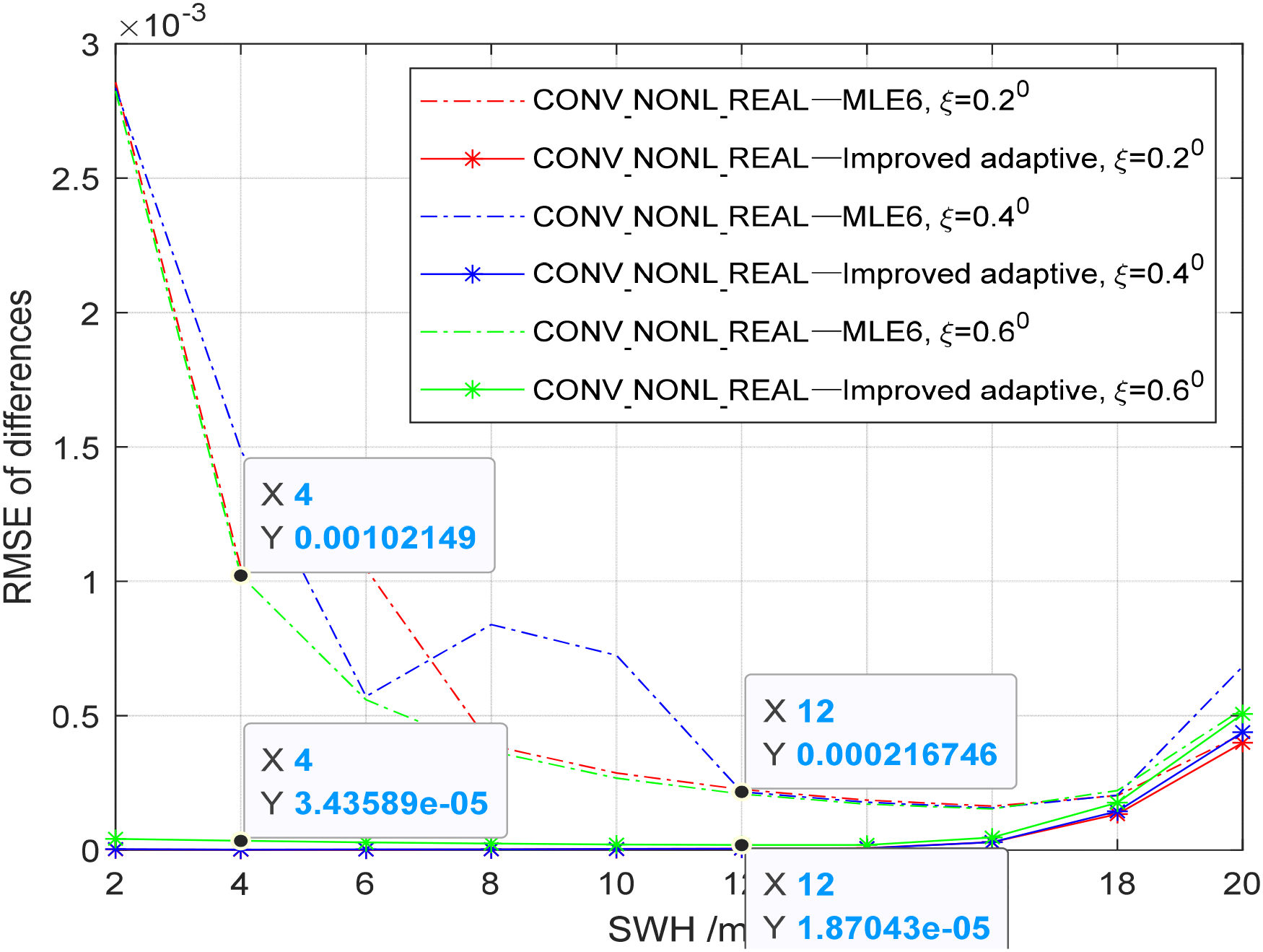
Differences among these simulated waveforms by MLE6/the improved adaptive algorithm and CONV_NONL_REAL varying with SWH.
4.2.2 Improved adaptive algorithm inverting SWH from SWIM measurements
The CONV_NONL_REAL model with non-Gaussian random ocean surface PDF and realistic radar PTR should be used to invert ocean parameters from SWIM measurements (waveforms). However, the three-term convolution model CONV_NONL_REAL will take a longer time than the improved adaptive algorithm to finish retracking these waveforms because of the great number of convolution operations.
The proposed improved adaptive algorithm was used to invert SWH from track Nos. 1–4 (https://aviso-data-center.cnes.fr/). The accuracy of inverting SWH can be considerably improved by 3–4 cm (Figure 21) when compared with that of the SWH inverted by the adaptive algorithm employed by SWIM. RMSE/Mean Bias of inverting SWH using the improved adaptive algorithm (0.25191 m/0.094783 m) was smaller than that of the adaptive algorithm used by SWIM from L2_file (0.26643 m/0.10947 m) (https://aviso-data-center.cnes.fr/), and the improvement was 1 cm for track No.1. For Track No. 2, RMSE/Mean Bias of inverting SWH using the improved adaptive algorithm (0.1865 m/0.074673 m) was smaller than that of the adaptive algorithm (0.23979 m/0.11979 m), and the improvement was 5 cm. For Track No.3, RMSE/Mean Bias of inverting SWH using the improved adaptive algorithm (0.15691 m/0.083337 m) was smaller than that of the adaptive algorithm (0.18493m/0.09788m), and the improvement was 3 cm. For Track No. 4, the RMSE/Mean Bias of inverting SWH by the improved adaptive algorithm (0.27555 m/0.11187 m) was smaller than that of the adaptive algorithm (0.31228 m/0.13348 m), and the improved amount was 4 cm. The mean total improvement was 3–4 cm. For these four tracks, the mean skewness parameter λs was estimated to be 0.11 or so.
Figure 21
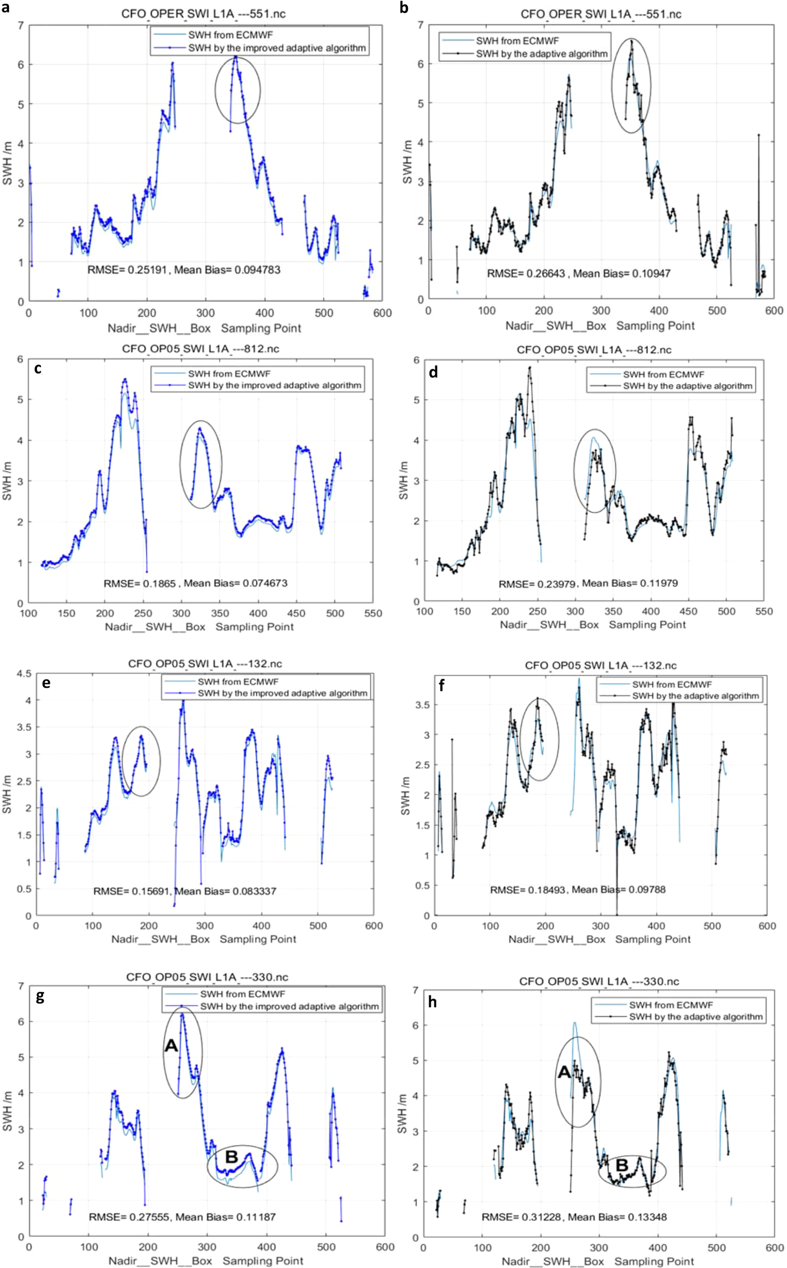
Retrieved SWH by the improved adaptive (a, c, e, g)/adaptive algorithm (b, d, f, h). Track No.1 (a, b), Track No.2 (c, d), Track No.3 (e, f), Track No.4 (g, h).
The improved adaptive algorithm presented in this article and the adaptive algorithm used by SWIM have the same PTR function. However, the improved adaptive algorithm accounts for the non-Gaussian effect, whereas the adaptive algorithm used by SWIM does not. Accounting for non-Gaussian effects can effectively improve the accuracy of inverting SWH, approximately 4 cm for SWIM. The case has the same principle as the above conclusion that MLE6 accounts for the non-Gaussian effect while MLE4 does not, and the mean improvement amount is 4 cm.
To better investigate the accuracy of the SWH inversion using the improved adaptive algorithm proposed in this paper, partial sea areas or specific SWH inversion data are selected for comparison and analysis, as shown by elliptical circles in Figures 21a–h. Except for the SWH retrieved in the sea area enclosed by the elliptical circle B (62 sampling points) in Track 4, all other retrieved results in those parts (31sampling points) enclosed by ellipses in Figure 21 show that the accuracy of the proposed improved adaptive algorithm retrieving SWH is significantly superior to that by the adaptive algorithm (Tourain et al., 2021) in the selected corresponding specific regions, as listed in Table 4A). The numerical value in the 32nd row represents the root mean square error (RMSE) of the data from the 1st to the 31st rows relative to the ECMWF values. The 33rd row of Table 4 is relative deviation. The proposed improved adaptive algorithm demonstrates remarkable improvement in higher sea states(SWH>3m), particularly when wave heights exceed 3 meters. In most cases, its relative deviation is less than 5%(4.18%, 7.52%, 2.17%, 4.63%), which is much lower than the inversion bias of significant wave height by multi-satellite data fusion and machine learning methods. Of course, the inversion deviation in these five sea areas is lower than that of the adaptive algorithm.
Table 4A
| Sampling Point | Track No.1: *551.nc file | Track No.2: *812.nc file | Track No.3: *132.nc file | ||||||
|---|---|---|---|---|---|---|---|---|---|
| ECMWF | Improved addaptive | Adaptive | ECMWF | Improved addaptive | Adaptive | ECMWF | Improved addaptive | Adaptive | |
| 1 | 4.74 | 4.453 | 4.582 | 2.51 | 2.697 | 1.673 | 2.20 | 2.289 | 2.131 |
| 2 | 5.16 | 5.481 | 4.999 | 2.56 | 2.768 | 1.913 | 2.18 | 2.274 | 2.121 |
| 3 | 5.38 | 5.619 | 5.443 | 2.7 | 2.898 | 2.176 | 2.16 | 2.259 | 2.113 |
| 4 | 5.66 | 5.879 | 5.601 | 2.83 | 3.079 | 2.395 | 2.20 | 2.269 | 2.166 |
| 5 | 5.83 | 6.023 | 5.654 | 3.05 | 3.320 | 2.669 | 2.23 | 2.293 | 2.253 |
| 6 | 6.04 | 6.162 | 5.731 | 3.27 | 3.513 | 2.816 | 2.25 | 2.292 | 2.150 |
| 7 | 6.13 | 6.190 | 5.669 | 3.50 | 3.753 | 2.910 | 2.25 | 2.289 | 2.072 |
| 8 | 6.16 | 6.364 | 6.105 | 3.74 | 4.027 | 3.133 | 2.25 | 2.312 | 2.052 |
| 9 | 6.20 | 6.319 | 6.212 | 3.89 | 4.152 | 3.329 | 2.29 | 2.328 | 2.128 |
| 10 | 6.17 | 6.416 | 6.252 | 4.01 | 4.286 | 3.501 | 2.35 | 2.374 | 2.178 |
| 11 | 6.11 | 6.360 | 6.578 | 4.06 | 4.361 | 3.688 | 2.41 | 2.460 | 2.375 |
| 12 | 6.06 | 6.208 | 6.541 | 4.07 | 4.394 | 3.685 | 2.49 | 2.467 | 2.482 |
| 13 | 5.94 | 6.010 | 6.355 | 4.07 | 4.344 | 3.543 | 2.57 | 2.597 | 2.425 |
| 14 | 5.82 | 5.942 | 5.717 | 4.01 | 4.267 | 3.511 | 2.63 | 2.631 | 2.472 |
| 15 | 5.75 | 5.889 | 5.458 | 3.98 | 4.255 | 3.746 | 2.71 | 2.691 | 2.452 |
| 16 | 5.69 | 5.859 | 5.261 | 3.94 | 4.201 | 3.424 | 2.77 | 2.756 | 2.556 |
| 17 | 5.61 | 5.766 | 5.264 | 3.93 | 4.162 | 3.218 | 2.78 | 2.784 | 2.573 |
| 18 | 5.55 | 5.923 | 5.437 | 3.9 | 4.082 | 3.448 | 2.78 | 2.768 | 2.686 |
| 19 | 5.44 | 5.688 | 5.364 | 3.86 | 4.060 | 3.607 | 2.80 | 2.809 | 2.762 |
| 20 | 5.33 | 5.460 | 5.471 | 3.77 | 3.998 | 3.546 | 2.87 | 2.859 | 2.850 |
| 21 | 5.18 | 5.316 | 5.483 | 3.66 | 3.908 | 3.416 | 2.90 | 2.907 | 2.822 |
| 22 | 5.07 | 5.348 | 5.206 | 3.55 | 3.780 | 3.771 | 2.92 | 2.959 | 2.873 |
| 23 | 4.94 | 5.253 | 5.234 | 3.41 | 3.667 | 3.322 | 2.98 | 3.001 | 3.031 |
| 24 | 4.82 | 5.123 | 5.237 | 3.24 | 3.513 | 3.237 | 3.11 | 3.116 | 3.225 |
| 25 | 4.72 | 4.887 | 4.674 | 3.10 | 3.361 | 3.202 | 3.18 | 3.209 | 3.468 |
| 26 | 4.63 | 4.803 | 4.566 | 2.93 | 3.198 | 3.162 | 3.22 | 3.305 | 3.467 |
| 27 | 4.53 | 4.891 | 4.842 | 2.77 | 3.022 | 2.868 | 3.26 | 3.313 | 3.608 |
| 28 | 4.45 | 4.641 | 5.192 | 2.58 | 2.841 | 2.379 | 3.27 | 3.333 | 3.430 |
| 29 | 4.38 | 4.603 | 4.513 | 2.41 | 2.681 | 2.379 | 3.21 | 3.280 | 3.447 |
| 30 | 4.30 | 4.554 | 4.533 | 2.29 | 2.526 | 2.483 | 3.14 | 3.264 | 3.233 |
| 31 | 4.21 | 4.480 | 4.557 | 2.23 | 2.455 | 1.951 | 3.05 | 3.189 | 3.094 |
| 32 | 0 | 0.224 | 0.294 | 0 | 0.252 | 0.422 | 0 | 0.058 | 0.155 |
| 33 | 0 | 4.18% | 5.5% | 0 | 7.52% | 12.61% | 0 | 2.17% | 5.76% |
SWH inversion in local sea areas enclosed by elliptical circles (m).
Table 4B
| Track No.4: *330.nc file, A | Track No.4: *330.nc file, B | Track No.4: *330.nc file, B | |||||||
|---|---|---|---|---|---|---|---|---|---|
| ECMWF | Improved addaptive | Adaptive | ECMWF | Improved addaptive | Adaptive | ECMWF | Improved addaptive | Adaptive | |
| 1 | 3.91 | 4.022 | 1.286 | 1.75 | 2.005 | 1.701 | 1.67 | 1.914 | 1.698 |
| 2 | 4.20 | 4.387 | 1.750 | 1.67 | 1.932 | 1.721 | 1.67 | 1.927 | 1.762 |
| 3 | 4.51 | 4.711 | 2.448 | 1.61 | 1.889 | 1.806 | 1.70 | 1.958 | 1.776 |
| 4 | 4.87 | 5.052 | 3.093 | 1.61 | 1.903 | 1.736 | 1.72 | 1.975 | 1.721 |
| 5 | 5.40 | 5.715 | 3.937 | 1.60 | 1.879 | 1.700 | 1.72 | 1.976 | 1.717 |
| 6 | 5.94 | 6.229 | 4.570 | 1.59 | 1.855 | 1.634 | 1.73 | 1.980 | 1.698 |
| 7 | 6.06 | 6.332 | 4.838 | 1.59 | 1.935 | 1.591 | 1.75 | 1.996 | 1.729 |
| 8 | 6.07 | 6.293 | 4.984 | 1.58 | 1.898 | 1.556 | 1.75 | 2.015 | 1.790 |
| 9 | 6.08 | 6.218 | 4.710 | 1.57 | 1.837 | 1.586 | 1.77 | 2.011 | 1.764 |
| 10 | 5.98 | 6.189 | 4.738 | 1.58 | 1.853 | 1.52 | 1.78 | 2.027 | 1.759 |
| 11 | 5.91 | 6.053 | 4.515 | 1.58 | 1.844 | 1.556 | 1.82 | 2.048 | 1.775 |
| 12 | 5.76 | 5.934 | 4.841 | 1.59 | 1.834 | 1.567 | 1.84 | 2.080 | 1.722 |
| 13 | 5.62 | 5.808 | 4.725 | 1.6 | 1.880 | 1.579 | 1.86 | 2.103 | 1.816 |
| 14 | 5.44 | 5.650 | 4.719 | 1.63 | 1.883 | 1.614 | 1.88 | 2.116 | 1.893 |
| 15 | 5.28 | 5.501 | 4.510 | 1.63 | 1.905 | 1.609 | 1.90 | 2.134 | 1.879 |
| 16 | 5.18 | 5.310 | 4.460 | 1.63 | 1.877 | 1.614 | 1.94 | 2.201 | 1.889 |
| 17 | 5.06 | 5.252 | 4.393 | 1.54 | 1.807 | 1.507 | 1.99 | 2.237 | 1.973 |
| 18 | 4.93 | 5.139 | 4.496 | 1.50 | 1.768 | 1.551 | 2.03 | 2.276 | 2.093 |
| 19 | 4.79 | 5.027 | 4.580 | 1.45 | 1.775 | 1.556 | 2.06 | 2.301 | 2.144 |
| 20 | 4.68 | 4.934 | 4.718 | 1.46 | 1.791 | 1.570 | 2.05 | 2.307 | 2.214 |
| 21 | 4.56 | 4.822 | 4.696 | 1.54 | 1.841 | 1.786 | 2.08 | 2.390 | 2.246 |
| 22 | 4.47 | 4.720 | 4.361 | 1.59 | 1.871 | 1.730 | 2.09 | 2.338 | 2.211 |
| 23 | 4.37 | 4.653 | 4.292 | 1.61 | 1.889 | 1.696 | 2.09 | 2.350 | 2.190 |
| 24 | 4.28 | 4.539 | 3.936 | 1.62 | 1.887 | 1.732 | 2.10 | 2.361 | 2.014 |
| 25 | 4.23 | 4.476 | 4.192 | 1.55 | 1.848 | 1.664 | 2.04 | 2.309 | 1.985 |
| 26 | 4.22 | 4.494 | 4.002 | 1.61 | 1.866 | 1.640 | 1.98 | 2.236 | 1.905 |
| 27 | 4.24 | 4.461 | 4.358 | 1.61 | 1.885 | 1.555 | 1.91 | 2.163 | 1.787 |
| 28 | 4.25 | 4.455 | 4.163 | 1.60 | 1.842 | 1.639 | 1.86 | 2.104 | 1.738 |
| 29 | 4.27 | 4.481 | 4.110 | 1.61 | 1.845 | 1.666 | 1.83 | 2.073 | 1.755 |
| 30 | 4.32 | 4.666 | 4.381 | 1.60 | 1.861 | 1.637 | 1.81 | 2.029 | 1.756 |
| 31 | 4.47 | 4.735 | 4.485 | 1.61 | 1.870 | 1.654 | 1.77 | 1.972 | 1.669 |
| 32 | 0 | 0.229 | 1.086 | 0 | 0.277 | 0.086 | 0 | 0.249 | 0.077 |
| 33 | 0 | 4.63% | 21.95% | 0 | 17.4% | 5.42% | 0 | 13.29% | 4.12% |
SWH inversion in local sea areas enclosed by elliptical circles (m).
In practices, a relatively complete model for inverting significant wave height (SWH) exhibits higher accuracy than multi-satellite data fusion (Qin and Li, 2021) and machine learning methods (Wang F. et al., 2022). This is because the SWH data inverted by each satellite remote sensor is obtained through model-based inversion, followed by certain corrections and processing. For instance, Janson, HY2, and SWIM all perform SWH inversion based on the MLE4 model. In general, the bias of retrieving SWH by using echo models (<0.5m or <5%) is lower than those empirical algorithms. Theoretical algorithms or model-based algorithms can serve as the foundation for empirical algorithms. From the inversion results of SWH derived from over 60,000 waveforms across these four orbits, when compared with ECMWF data, the deviations (RMSE) of both algorithms are less than 0.31 meters, which is smaller than those of data fusion and neural network inversion methods (Qin and Li, 2021; Wang F. et al., 2022).
Compared with the vast expanse of the ocean, the coverage of satellites’footprint is limited. Using machine learning or multi-data fusion methods to infer the significant wave height in unknown sea areas is a rapid approach, but the accuracy cannot be guaranteed. This is due to the high spatiotemporal variability characteristics of the ocean. These empirical algorithms are necessary to be validated furtherly in those unknown regions.
In Figure 21, at lower sea states (especially when SWHs are below 2 meters), the improvement of the improved adaptive model becomes less pronounced, which is attributed to the algorithm’s and sampling points’ lower resolution in such condition. When SWH is very small, the leading edge of the echo waveform, related to SWH, is steep. Due to nonlinear effects of the roughly sea surfaces, the leading edge of the waveform changes drastically in a certain degree, as shown in Figure 19. And thus, the insufficient sampling points and algorithm’s lower resolution will lead to less improvement in the inversion of SWH. For the special region B in Figure 21g, the relative deviation is more than 10%(17.4%,13.29%) although RMSE is less than 0.30m(0.277m, 0.249m).
5 Conclusions
In this study, we explored the improved second-order retracking algorithm known as MLE6, which incorporates the SB coefficient (λs) and EMB coefficient (λem). The upgraded algorithm MLE6 addresses the non-Gaussian effects of a random ocean, in contrast to the current operational algorithm MLE4, which disregards the impact of non-linear or non-Gaussian rough ocean surfaces on SWH inversion. MLE6 is different from MLE4 when λs and λem are not equal to zero but it matches MLE4 when λs = 0 and λem = 0. The coefficient (λs) distorts the return waveform shape, particularly the leading edge, which has an effect on SWH inversion.
First, the performance of MLE6 was analyzed. The return waveforms simulated by MLE6 were studied and found to be closer to those of the three-term convolution model CONV_NONL than to MLE4 (Figure 4). RMSE_waveform of differences between MLE6 and CONV_NONL (an average value of 6.76 × 10⁻⁵ normalized unit) were smaller than that between MLE4 and CONV_NONL (an average value of 1.70 × 10⁻³ normalized unit). Compared with MLE4, MLE6 is almost identical to the three-term convolution model CONV_NONL and can replace CONV_NONL in inverting SWH from the return waveforms measured by SRA or SWIM. By retracking the return waveforms simulated by CONV_NONL, MLE6 can have better accuracy in inverting SWH than MLE4, with an improvement of approximately 3–7 cm and a mean value of 3.163 cm. The improvement increased as the mispointing angle increased, reaching a peak when the mispointing angle was less than 0.4°, but remained almost unchanged when the mispointing angle exceeded 0.4°.
We applied the improved technique MLE6 to inverting SWH from SWIM measurements at the nadir. The inverted results showed that MLE6 had higher accuracy in inverting SWH compared to MLE4, with an improvement of 3–5 cm in RMSE and Mean Bias when using ECMWF as a benchmark. Results obtained from the situ data aligned with those from simulated waveforms.
Although the PDF of MLE6 differed from that of MLE4, the PTR functions of both models were similar, approximately Gaussian distributions due to the difficulty in measuring the realistic PTR of a remote sensor. However, the realistic PTR of the SWIM instrument was measured and could be obtained from CFOSAT. And thus an improved adaptive algorithm was introduced in this study to consider the realistic PTR of the SWIM instrument. The PDF of the improved adaptive algorithm, accounting for the non-Gaussian effects on inverting SWH, was different from that of the adaptive algorithm used by SWIM, despite having the same PTR function. The improved adaptive algorithm was nearly identical to CONV_NONL_REAL, with the similar non-Gaussian PDF and realistic PTR. The difference in RMSE between the two models (10−5 normalized unit) was smaller than that between the adaptive algorithm and CONV_NONL_REAL (10−3 normalized unit). Due to accounting for the non-Gaussian random ocean and realistic radar PTR, the proposed improved adaptive algorithm could more effectively invert ocean parameters than the adaptive algorithm.
The improved adaptive algorithm was applied to invert SWH from the same four-track measurements of SWIM. Using ECMWF measurements as references. It effectively enhanced the accuracy of inverting SWH by 3–4 cm compared to the adaptive algorithm employed by SWIM.
MLE6, which addresses non-Gaussian effects on estimating SWH, and the improved adaptive algorithm, considering non-Gaussian random ocean surface and realistic radar PTR, were validated, showing better accuracy in inverting SWH than MLE4 and the adaptive algorithm used by SWIM. Both algorithms have the potential to replace MLE4 or other retracking algorithms for inverting ocean parameters (e.g., SWH) in future altimeter missions.
The Nelder Mead algorithm, sensitive to initial value selection, is a local optimal algorithm that is prone to getting stuck in local minima and requires strict initial value settings. If the initial value is set incorrectly, there may be a significant deviation in the inverted SWH. Exploring global optimal algorithms or finding a good suitable algorithm for the improved adaptive model will be a future mission.
Beyond the altimeter data employed in this study, future research on significant wave height (SWH) can explore the potential of recent advancements in radar systems and deep learning methods. For example, novel radar technologies, such as the SAR altimeter (Jiang et al., 2020), may offer innovative approaches to SWH measurement and inversion. Some unique signal processing capabilities can potentially yield more detailed and accurate insights into wave characteristics, particularly regarding Doppler scattering mechanisms (Zhang et al., 2024) associated with SWH. Deep learning has shown remarkable promise in various remote-sensing applications, holding the potential to revolutionize SWH research. Specifically, some remote-sensing images (Gao et al., 2025) incorporating contextual global attention mechanisms and lightweight task-specific context decoupling, can inspire new ideas for SWH research. The concept of using multi-source data can be applied to SWH research. By fusing data from satellite altimeters, radar systems, and in-situ sensors, researchers can achieve a more comprehensive and precise understanding of SWH. This multi-source data approach not only mitigates the limitations of individual data sources but also enhances the overall reliability of SWH estimations.
Statements
Data availability statement
The original contributions presented in the study are included in the article/Supplementary Material. Further inquiries can be directed to the corresponding author.
Author contributions
JT: Conceptualization, Funding acquisition, Investigation, Methodology, Writing – original draft, Writing – review & editing. JW: Conceptualization, Methodology, Software, Writing – original draft, Writing – review & editing. JS: Methodology, Software, Writing – original draft, Writing – review & editing, Data curation, Investigation, Validation.
Funding
The author(s) declare that financial support was received for the research and/or publication of this article. This work was project 2023CFO012 supported by the Key Laboratory of Space Ocean Remote Sensing and Application, MNR. This Project was partially supported by the National Natural Science Foundation of China (grant number 41876104).
Acknowledgments
This work was project 2023CFO012 supported by the Key Laboratory of Space Ocean Remote Sensing and Application, MNR. This Project was partially supported by the National Natural Science Foundation of China (grant number 41876104). Thank ECMWF.
Conflict of interest
The authors declare that the research was conducted in the absence of any commercial or financial relationships that could be construed as a potential conflict of interest.
Generative AI statement
The author(s) declare that no Generative AI was used in the creation of this manuscript.
Publisher’s note
All claims expressed in this article are solely those of the authors and do not necessarily represent those of their affiliated organizations, or those of the publisher, the editors and the reviewers. Any product that may be evaluated in this article, or claim that may be made by its manufacturer, is not guaranteed or endorsed by the publisher.
References
1
Abdalla S. (2013). Evaluation of radar altimeter path delay using ECMWF pressure-level and model-level fields (Shinfield Park, Reading, RG2 9AX, England: Series: ECMWF - ESA Contract Report), 1–26. Available online at: http://www.ecmwf.int/publications/
2
Amarouche L. Thibaut P. Zanife O. Z. Dumon J.-P. Vincent P. Steunou N. (2004). Improving the jason-1 ground retracking to better account for attitude effects. Mar. Geodesy27, 171–197. doi: 10.1080/01490410490465210
3
Brown G. (1977). The average impulse response of a rough surface and its applications. IEEE Trans. Antennas Propagation25, 67–74. doi: 10.1109/TAP.1977.1141536
4
Cao C. Bao L. Cao G. Liu G. Zhang X. (2024). A novel method for ocean wave spectra retrieval using deep learning from sentinel-1 wave mode data. IEEE Trans. Geosci. Remote Sens.62, 4204016(1–16). doi: 10.1109/TGRS.2024.3369080
5
Chelton B. Ries J. C. Haines B. J. Fu L. L. Callahan P. S. (2001). “Chapter 1 satellite altimetry,” in Satellite Altimetry and Earth Sciences, vol. 69. Eds. FuL.-L.CazenaveA. (Pasadena, California: Jet Propulsion Laboratory California Institute of Technology), 1–ii. doi: 10.1016/S0074-6142(01)80146-7
6
Fu L.-L. Cazenave A. (2001). Satellite Altimetry and Earth Sciences: A Handbook of Techniques and Applications (San Diego: Academic Press).
7
Gao G. Wang M. Zhang X. Li G. (2025). DEN: A new method for SAR and optical image fusion and intelligent classification. IEEE Trans. Geosci. Remote Sens.63, 201118(1–18). doi: 10.1109/TGRS.2024.3500036
8
Gao G. Yao B. X. Li Z. Y. Duan D. F. Zhang X. (2024). Forecasting of sea surface temperature in eastern tropical pacific by a hybrid multiscale spatial–temporal model combining error correction map. IEEE Trans. Geosci. Remote Sens.62, 4204722(1–22). doi: 10.1109/TGRS.2024.3353288
9
Gaspar P. Labroue S. Ogor F. Lafitte G. Marchal L. Rafanel M. et al . (2002). Improving nonparametric estimates of the sea state bias in radar altimeter measurements of sea level. J. Atmospheric Oceanic Technol.19, 1690–1707. doi: 10.1175/1520-0426(2002)0192.0.co;2
10
Ge H. Li B. Jia S. Nie L. Wu T. Yang Z. et al . (2022). LEO Enhanced Global Navigation Satellite System (LeGNSS): progress, opportunities, and challenges. Geo-spatial Inf. Sci.25, 1–13. doi: 10.1080/10095020.2021.1978277
11
Guan Y. Zhang X. Gao G. Cao C. Li Z. Fu S. et al . (2025). A new indicator for assessing fishing ecological pressure using multi-source data: A case study of the South China Sea. Ecol. Indic.170, 113096. doi: 10.1016/j.ecolind.2025.113096
12
Hauser D. Tourain C. Hermozo L. Alraddawi D. Aouf L. Chapron B. et al . (2020). New observations from the SWIM radar on-board CFOSAT: instrument validation and ocean wave measurement assessment. IEEE Trans. Geosci. Remote Sens.PP, 1–22. doi: 10.1109/TGRS.2020.2994372
13
Hayne G. S. (1980). Radar altimeter mean return waveforms from near-normal-incidence ocean surface scattering. IEEE Trans. Antennas Propagation28, 687–692. doi: 10.1109/TAP.1980.1142398
14
He-Guang L. Xi-Yu X. Le Y. (2018). “Analysis of the dependence on retrackers of the jason satellites altimetry products,” in IGARSS 2018 - 2018 IEEE International Geoscience and Remote Sensing Symposium, 1 July 2018. Valencia, Spain: IGARSS 2018, 7672–7675. doi: 10.1109/IGARSS.2018.8518162
15
Huang X. Miao H. Xue W. Miao X. Wang G. . (2019). “Study on neutral networks of ionosphere delay corrections of satellite altimeters,” in IGARSS 2019 - 2019 IEEE International Geoscience and Remote Sensing Symposium (Yokohama, Japan: IEEE), 8286–8289. doi: 10.1109/IGARSS.2019.8898329
16
Jiang L. Nielsen K. Dinardo S. Andersen O. B. Bauer-Gottwein P. (2020). Evaluation of Sentinel-3 SRAL SAR alitimetry over Chinese rivers. Remoter. Sens. Environ.237, 111546. doi: 10.1016/j.rse.2019.111546
17
Jiang M. Xu K. Xu X. Shi L. Yu X. Liu P. (2019). “Range noise level estimation of HY-2b radar altimeter and its comparison with jason-2 and jason-3 altimeter,” in IGARSS 2019 - 2019 IEEE International Geoscience and Remote Sensing Symposium, Yokohama, Japan, 1 July 2019. 8312–8315. doi: 10.1109/IGARSS.2019.8898503
18
Kang Z. Bettadpur S. Nagel P. Save H. Poole S. Pie N. . (2020). GRACE-FO precise orbit determination and gravity recovery. J. Geodesy94, 1–17. doi: 10.1007/s00190-020-01414-3
19
Labroue S. Gaspar P. Dorandeu J. et al . (2004). Nonparametric estimates of the sea state bias for the jason-1 radar altimeter. Mar. Geodesy17, 453–481. doi: 10.1080/01490410490902089
20
Lago L. S. Saraceno M. Ruiz-Etcheverry L. A. Passaro M. Oreiro F. A. D’Onofrio E. E. et al . (2017). Improved sea surface height from satellite altimetry in coastal zones: A case study in southern patagonia. IEEE J. Selected Topics Appl. Earth Observations Remote Sens.10, 3493–3503. doi: 10.1109/JSTARS.2017.2694325
21
Li X. Xu Y. Liu B. Lin W. He Y. Liu J. (2021). Validation and calibration of nadir SWH products from CFOSAT and HY-2B with satellites and in situ observations. J. Geophysical Res.: Oceans126, 1–16. doi: 10.1029/2020JC016689
22
Li X. Zhang K. Zhang Q. Zhang W. Yuan Y. Li X. et al . (2018). Integrated orbit determination of fengyun-3c, bds, and gps satellites. J. Geophysical Res. Solid Earth123, 8143–8160. doi: 10.1029/2018jb015481
23
Millet F. W. Arnold D. V. Warnick K. F. Smith J. (2003). Electromagnetic bias estimation using in situ and satellite data: 1. rms wave slope. J. Geophysical Res. Oceans108, C001095. doi: 10.1029/2001jc001095
24
Montenbruck O. Hackel S. Jaggi A. (2018). Precise orbit determination of the sentinel-3a altimetry satellite using ambiguity-fixed gps carrier phase observations. J. Geodesy92, 711–726. doi: 10.1007/s00190-017-1090-2
25
Nelder J. A. Mead R. (1965). A simplex method for function minimization. Comput. J.7, 308–313. doi: 10.1093/comjnl/7.4.308
26
Peacock N. R. Laxon S. W. (2004). Sea surface height determination in the Arctic Ocean from ERS altimetry. J. Geophysical Res.109, 1–14. doi: 10.1029/2001JC001026
27
Qin L. Li Y. (2021). Significant wave height estimation using multi-satellite observations from GNSS-R. Remote Sens.13, 4806(1–48010). doi: 10.3390/rs13234806
28
Richard C. (2001). Satellite altimetry and earth sciences: A handbook of techniques and applications. EOS Trans. Am. Geophysical Union82, 376–376. doi: 10.1029/01EO00233
29
Rodríguez E. (1988). Altimetry for non-Gaussian oceans: Height biases and estimation of parameters. J. Geophysical Res.: Oceans93, 14107–14120. doi: 10.1029/JC093iC11p14107
30
Rosmorduc V. Benveniste J. Bronner E. Dinardo S. Picot N. . (2018). Radar Altimetry Tutorial. Available online at: http://www.altimetry.info (Accessed September 2011).
31
Rossi L. C. (2003). TOPEX Project Radar Altimeter Development Requirements and Specifications. Version 6.0, June 2003 (USA: NASA, TOPEX Project Office). (Accessed September 2011).
32
Thibaut P. Amarouche L. Ferreira F. Zanife O. Z. Vincent P. . (2005). “Estimation of the skewness coefficient using Jason-1 altimeter data,” in IEEE International Geoscience & Remote Sensing Symposium, IEEE, July 2005. (Seoul, Korea South, IGARSS 2005) 2556–2559. doi: 10.1109/IGARSS.2005.1525506
33
Thibaut P. Poisson J. C. Bronner E. Picot N. (2010). Relative performance of the MLE3 and MLE4 retracking algorithms on jason-2 altimeter waveforms. Mar. Geodesy33, 317–335. doi: 10.1080/01490419.2010.491033
34
Tian J. Shi J. (2023). High-precision retrieving ocean parameters based on a new improved second-order model with considering non-gaussian effects. IEEE Geosci. Remote Sens. Lett.20, 1–5, 1503405. doi: 10.1109/LGRS.2023.3321739
35
Tourain C. Piras F. Ollivier A. Hauser D. Poisson J. C. Boy F. et al . (2021). Benefits of the Adaptive algorithm for retracking altimeter nadir echoes: results from simulations and CFOSAT/SWIM observations. IEEE Trans. Geosci. Remote Sens.59, 9927–9940. doi: 10.1109/TGRS.2021.3064236
36
Tran N. Vandemark D. Labroue S. Feng H. Chapron B. Tolman H. L. et al . (2010). Sea state bias in altimeter sea level estimates determined by combining wave model and satellite data. J. Geophysical Res.: Oceans115, c03020.1–7. doi: 10.1029/2009JC005534
37
Wang F. Yang D. Yang L. (2022). Retrieval and assessment of significant wave height from CYGNSS mission using neural network. Remote Sens.14, 3666(1–36619). doi: 10.3390/rs14153666
38
Wang Y. Li M. Jiang K. Li W. Zhao Q. Peng H. et al . (2022). Precise orbit determination of the Haiyang 2C altimetry satellite using attitude modeling. GPS Solutions26, 1–14. doi: 10.1007/s10291-021-01219-7
39
Zhang X. Gao G. Chen S.-W. (2024). Polarimetric autocorrelation matrix: A new tool for joint characterizing of target polarization and doppler scattering mechanism. IEEE Trans. Geosci. Remote Sens.62, 5213522(1–22). doi: 10.1109/TGRS.2024.3398632
Summary
Keywords
altimeter, swim, significant wave height, ocean observation, non-linear ocean
Citation
Tian J, Wang J and Shi J (2025) Performance analysis of the improved second-order retracking algorithm and its application for significant wave height estimation. Front. Mar. Sci. 12:1569799. doi: 10.3389/fmars.2025.1569799
Received
01 February 2025
Accepted
19 June 2025
Published
23 July 2025
Volume
12 - 2025
Edited by
Xi Zhang, Ministry of Natural Resources, China
Reviewed by
Chenqing Fan, Ministry of Natural Resources, China
Hongli Miao, Ocean University of China, China
Updates
Copyright
© 2025 Tian, Wang and Shi.
This is an open-access article distributed under the terms of the Creative Commons Attribution License (CC BY). The use, distribution or reproduction in other forums is permitted, provided the original author(s) and the copyright owner(s) are credited and that the original publication in this journal is cited, in accordance with accepted academic practice. No use, distribution or reproduction is permitted which does not comply with these terms.
*Correspondence: Jiasheng Tian, tianjs@hust.edu.cn
Disclaimer
All claims expressed in this article are solely those of the authors and do not necessarily represent those of their affiliated organizations, or those of the publisher, the editors and the reviewers. Any product that may be evaluated in this article or claim that may be made by its manufacturer is not guaranteed or endorsed by the publisher.