INCOIS air-sea Flux Reference System onboard ORV Sagar Nidhi: overview and initial results

Accurate estimation of air-sea fluxes is essential for advancing ocean modeling, observational studies, and understanding air-sea interactions. To address this need, the Indian National Centre for Ocean Information Services (INCOIS) developed and deployed a Flux Reference System (INCOIS-FRS) onboard ORV Sagar Nidhi. This article provides an overview of the system, its components, data acquisition methods, flux computation techniques, and preliminary results. The INCOIS-FRS integrates an Eddy Covariance Flux System (ECFS) and an Automated Weather Station (AWS). The ECFS collects high-frequency (20 Hz) data to directly estimate the latent heat flux (LHF), sensible heat flux (SHF), and momentum flux (τ) using the Eddy Covariance (EC) method. The AWS records meteorological and oceanic variables at 1 Hz, enabling flux estimates using the COARE 3.5 algorithm. A spectrally flat Class-A pyranometer and a pyrgeometer provide climate-grade measurements of downward shortwave and longwave radiation, which, combined with EC-derived SHF and LHF, yield the net heat flux. This article presents preliminary results inferred from data collected by INCOIS-FRS during a cruise in the Arabian Sea from 1–16 July 2023. Data from this system are useful for validating model outputs and satellite observations, refining flux parameterizations, marine boundary layer studies, and improving air-sea interaction models. INCOIS-FRS represents a first step toward equipping more oceanographic platforms, both crewed and uncrewed, with flux reference units. Future plans include expanding such deployments to enhance observational coverage and support research on air-sea fluxes across the Indian Ocean and other regions.

1 Introduction

The exchange of momentum, heat, and gases at the air-sea interface is a fundamental process driving the coupled ocean-atmosphere system, with implications for weather, climate variability, and ocean circulation (Garbe et al., 2014; Cronin et al., 2019). Turbulence plays a critical role in mediating these exchanges, yet the complex and multi-scale nature of turbulent processes over the open ocean poses significant observational challenges. While controlled laboratory experiments provide valuable insights, direct measurements of turbulent fluxes in the marine environment are essential for accurately quantifying air-sea interactions and improving our understanding of ocean-atmosphere coupling (Fairall et al., 2003).

Air-sea flux measurements can be achieved using the eddy covariance (EC) method, which provides the most direct measure of turbulent heat and momentum fluxes (Edson et al., 1998). However, the availability of such direct flux measurements remains limited to a few locations, primarily on moored buoys, restricting their global coverage (Cronin et al., 2019). Consequently, air-sea fluxes are often estimated using bulk flux parameterizations, which, despite their utility, introduce significant uncertainties due to their non-linear nature. These uncertainties can result in imbalances in basin-scale heat flux estimates (Kato et al., 2013; Valdivieso et al., 2017). Errors in air-sea flux forcing can profoundly impact ocean heat redistribution processes—such as convection, stratification, and large-scale circulation—compromising the detection and interpretation of climate change signals (Storto et al., 2018; Carton et al., 2018). Reducing these uncertainties remains a critical challenge for numerical ocean models, climate monitoring (Hakuba et al., 2024), and operational forecasting (Martin et al., 2007; Storto et al., 2019).

Global initiatives like the Global Tropical Moored Buoy Array (GTMBA) have transformed the availability of in-situ ocean-atmosphere observations in tropical regions (McPhaden et al., 2010, 2023). This multinational program began with the TAO/TRITON array in the Pacific, which currently maintains 67 moorings (McPhaden et al., 1998). PIRATA, launched in the Atlantic in the mid-1990s, now includes 19 moorings (Bourlès et al., 2008), while RAMA, established in the Indian Ocean to study the Asian monsoon variability, operates 29 moorings (McPhaden et al., 2009). These arrays provide real-time data that have significantly advanced our understanding of climate variability, ocean dynamics, and forecasting capabilities. However, since much of the GTMBA data is assimilated into reanalysis products, its value as an independent validation dataset is limited. To address the need for unassimilated reference data, the OceanSITES network was established (Send et al., 2010), providing high-quality in situ datasets that serve as essential benchmarks for validating air-sea fluxes.

Though the data from GTMBA and OceanSITES networks have improved the flux accuracy, process-specific observations are still essential to refine flux parameterizations under varied atmospheric and oceanic conditions. Extensive EC data collection efforts in the West Pacific, Atlantic, and extratropical regions have contributed to significant advancements in air-sea flux algorithms. For example, the widely used COARE bulk flux models (versions 2.5, 3 and 3.5) were developed based on these datasets. More recently, the South China Sea has emerged as an important region for such observations, yielding new insights into the role of marine atmospheric boundary layer stability, mean winds, and sea state on flux exchanges (Chen et al., 2019, 2020). Despite these advances, there is still a lack of consensus regarding the relative importance of these factors. Some studies emphasize the dominant role of atmospheric stability and mean surface winds (Fairall et al., 1996, 2003; Edson et al., 2013; Santini et al., 2020), while others highlight the influence of sea state, particularly under low or very high wind conditions (Oost et al., 2002; Drennan et al., 2003; Pezzi et al., 2016; Hackerott et al., 2018; Sauvage et al., 2023; Raj et al., 2024).

In the Indian Ocean, fundamental studies on air-sea flux parameterizations remain limited due to the scarcity fine-scale EC flux measurements. Early efforts to collect EC data were undertaken during the Bay of Bengal Monsoon Experiment (BOBMEX) in 1999, which recorded 10-Hz flux measurements during the summer monsoon (Bhat, 2003). This was followed by the Ocean Mixing and Monsoon (OMM) program initiated by the Ministry of Earth Sciences (MoES, Government of India), which collected 16 months of EC data in the Bay of Bengal (Raj et al., 2024), marking a significant step toward advancing air-sea flux research in the region. However, these efforts were geographically limited, focusing primarily on measurements in the Bay of Bengal, and lacked broader spatial coverage.

To overcome these limitations in data collection, the Indian National Centre for Ocean Information Services (INCOIS) developed and installed a Flux Reference System (INCOIS-FRS) onboard the ORV Sagar Nidhi. The INCOIS-FRS comprises an Eddy Covariance Flux System (ECFS) and an Automated Weather Station (AWS) mounted on a bow mast, enabling the continuous collection of high-quality flux observations along the ship’s route. This system represents a significant step in addressing the need for high-accuracy, process-specific flux measurements in the Indian Ocean.

This article describes the INCOIS-FRS and its components, detailing the system design, data processing algorithms, and some preliminary results. Section 2 describes the system, while Section 3 outlines the data processing methodology. Initial findings from the flux observations collected during the summer monsoon of 2023 in the Arabian Sea are presented in Section 4. Finally, Section 5 summarizes the key points and highlights the importance of this system for advancing air-sea flux research in the Indian Ocean.

2 Flux reference system

The FRS installed onboard ORV Sagar Nidhi consists of two components: the Eddy Covariance Flux System and an AWS. Figure 1 shows the distance view illustration of the ORV Sagar Nidhi bow mast and the instruments on top. Detailed descriptions of these systems are provided below.

Figure 1

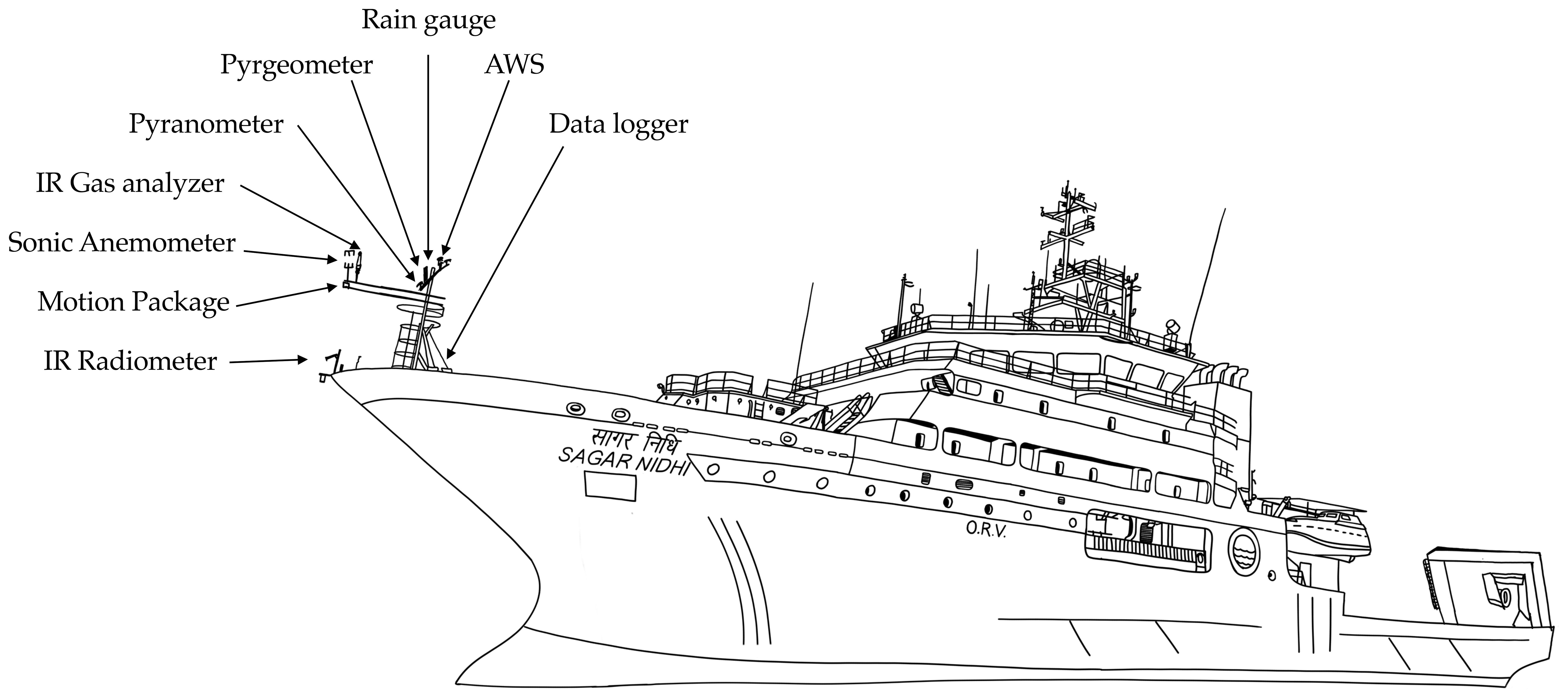
Figure 1. Illustration of ORV-Sagar Nidhi featuring bow mast with INCOIS-FRS instruments.

2.1 Eddy covariance flux system

The Eddy Covariance Flux System (ECFS) measures horizontal and vertical wind components in ship-based coordinates using a 3-axis Gill R3–50 sonic anemometer. Additionally, the sonic anemometer records the speed of sound to calculate the sonic temperature, which is equivalent to the virtual temperature. The Licor LI7500-RS Infrared Gas Analyzer (IRGA) records gas concentrations for scalar flux measurements. The system also includes the Inertial Motion Unit (IMU) – Microstrain 3DM-GX5-35, which tracks 3-axis platform motion through linear accelerometers, angular rate sensors, and a magnetometer.

The ECFS sensors are mounted on the bow mast at a height of 15 m above the mean sea level. The IRGA and sonic anemometer are fixed to a horizontal bar structure aligned with the ship’s bow. A horizontal separation of 30 cm is maintained between the IRGA and the sonic anemometer to ensure accurate flux measurements. This separation optimizes the covariance between scalar concentrations and vertical wind fluctuations while avoiding airflow disruptions caused by sensor proximity. The sonic anemometer is oriented with its ‘system north’ aligned with the ship’s bow and follows a righthanded (x, y, z) coordinate system with x positive forward (to bow), y positive to port, z positive upward. It enables measurements to be initially referenced in ship-based coordinates and later converted to earth-referenced coordinates during post-processing. The IMU, mounted directly beneath the sonic anemometer, provides ship motion information necessary for correcting sonic wind components. All ECFS data are collected at a sampling rate of 20 Hz and stored in 20-minute discrete files in a Campbell Scientific CR1000X data logger. The detailed list of variables recorded by the ECFS is provided in Table 1.

Table 1

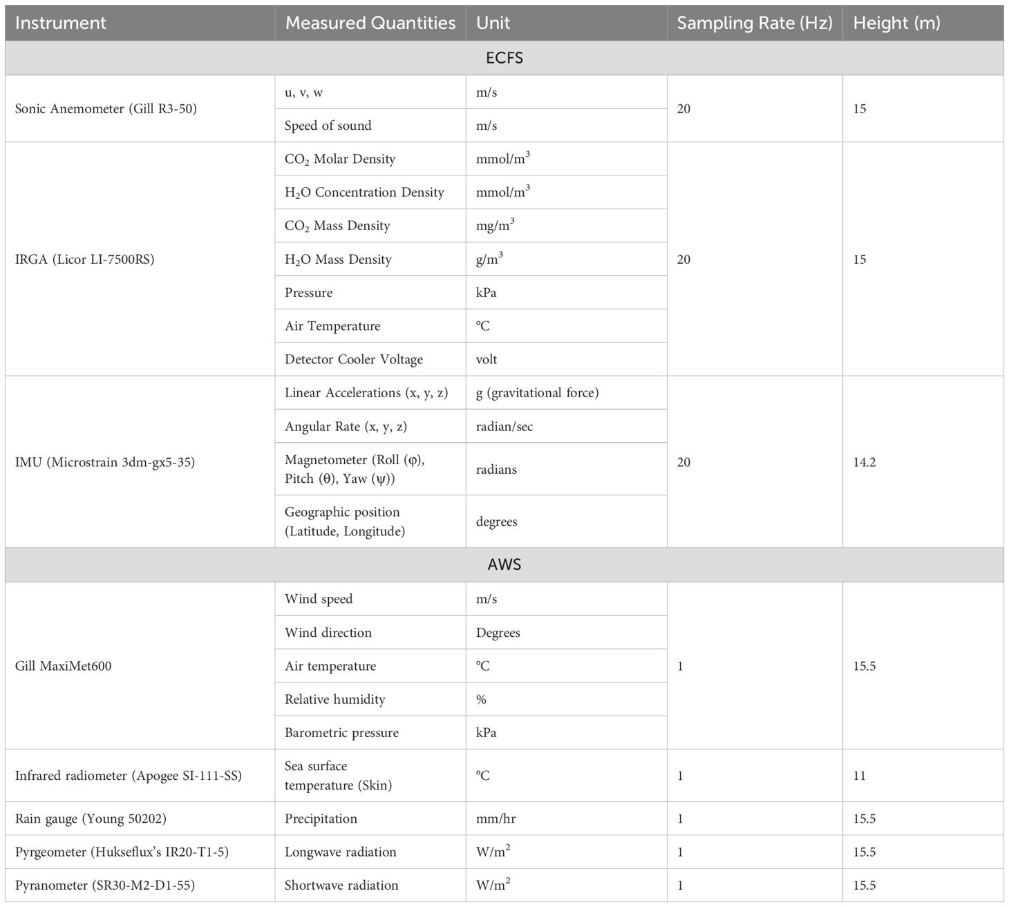
Table 1. Sensor model details and the measured quantities of INCOIS-FRS.

2.2 The automated weather station

The AWS consists of five sensors integrated into the Gill MaxiMet600 compact weather station. It measures wind speed, wind direction, air temperature, relative humidity, and barometric pressure. With GPS integration, the station provides corrected wind speed and direction relative to ship movement. Additionally, hourly cumulative rainfall is measured using a Young 50202 precipitation gauge. With no moving parts, this gauge is particularly well-suited for shipboard precipitation measurements.

Unlike most shipboard AWS setups, the INCOIS-FRS also incorporates an Apogee SI-111-SS infrared radiometer to measure the skin sea surface temperature ($SS{T}_{skin}$). The radiometer is mounted on the bow railing at a height of 10 m above the sea surface and angled 22° downward. This configuration allows the radiometer to have a 67 m² field of view (FOV) over the sea surface. For radiation measurements, the system uses Hukseflux’s spectrally flat Class-A pyranometer SR30-M2-D1–55 and IR20-T1–5 pyrgeometer to capture shortwave and longwave radiation respectively. The spectrally flat, Class-A type pyranometers measure the highest accuracy, climate-scale accuracy shortwave radiation measurements.

2.3 Turbulent air-sea fluxes calculation methods

Three commonly used methods for estimating air-sea fluxes are the Eddy Covariance (EC) method, the Inertial Dissipation Method (IDM), and the bulk method. Each approach has its own advantages and limitations, as detailed below.

2.3.1 Eddy covariance

The EC method is the most direct way of estimating turbulent fluxes, and it computes them as the covariance between vertical fluctuations of velocity and scalar quantity of interest (Edson et al., 1998). Turbulent fluxes from EC method are written as

$\begin{array}{ll}\text{τ}=-\text{ρ}\hspace{0.17em}\overline{u^{\prime }{w}^{\prime }} \widehat{i}-\text{ρ}\hspace{0.17em}\overline{v^{\prime }{w}^{\prime }} \widehat{j}& (1)\end{array}$

$\begin{array}{ll}H=\text{ρ}{C}_p\overline{w^{\prime }{\theta }^{\prime }}& (2)\end{array}$

$\begin{array}{ll}E=\text{ρ}{L}_e\overline{w^{\prime }{q}^{\prime }}& (3)\end{array}$

where Equations 1–3 represent momentum flux (τ), sensible heat flux (H), and latent heat fluxes (E). Here ρ is the density of air, C ${ }_p$ is the specific heat of air at constant pressure, $L_e$ is the latent heat of evaporation of water, and ${\theta }^{\prime }$ and $q^{\prime }$ denote fluctuations in potential temperature and specific humidity, respectively. More details about the EC calculation followed for INCOIS-FRS are described in section 3.

2.3.2 Inertial dissipation method

The IDM follows the Taylor hypothesis as turbulence is considered frozen when it moves past the sensor and the dissipation rate of Turbulent Kinetic Energy (TKE) can be derived from the power spectral density of downstream wind components (Pond et al., 1971; Hicks and Dyer, 1972; Edson et al., 1991). This method has been used extensively to estimate fluxes over various scenarios using data from buoys, ships, and aircraft (Pond et al., 1971; Large and Pond, 1981). The normalized TKE equation during stationary and horizontally homogeneous conditions can be written as

$\begin{array}{ll}\underset{P}{\underbrace{\frac{kz}{u_{*}^3}\left(\overline{u^{\prime }{w}^{\prime }}\frac{\partial \overline{u}}{\partial z}\right)}}-\underset{B}{\underbrace{\frac{kz}{u_{*}^3}\frac{g}{T_0}\overline{w^{\prime }{\theta }_v^{"}}}}-\underset{Tt}{\underbrace{\frac{kz}{u_{*}^3}\frac{\partial \overline{w^{\prime }e}}{\partial z}}}+\underset{Tp}{\underbrace{\frac{kz}{u_{*}^3}\left(\frac{1}{\rho }\right)\frac{\partial \overline{p^{\prime }{w}^{\prime }}}{\partial z}}}-\underset{D}{\underbrace{\frac{kz}{u_{*}^3}ϵ}}=0& (4)\end{array}$

Where $e=0.5(u^{\text{'}2}+v^{\text{'}2}+w^{\text{'}2})$, $\overline{w^{\prime }{\theta }_{\text{v}}^{\prime }}$ is the flux of virtual potential temperature, $T_0$ is a reference temperature in the surface layer, $k$ is the von Karman constant (0.4), $g$ the acceleration due to gravity, $z$ is the height of the measurements, and $L$ is the Obukhov length. Term (P) corresponds to the normalized mechanical production of TKE from the mean flow, (B) is the normalized buoyant production or loss term, Tt and Tp are the normalized turbulence and pressure transport terms, respectively, and (D) is the normalized molecular dissipation of TKE.

Under the classical IDM method, the transport terms are neglected, either they are very small, or they tend to cancel each other, and the TKE budget assumes a balance to total production of TKE with dissipation (Champagne et al., 1977; McBean and Elliott, 1975). Under these assumptions, neglecting the transport terms, Equation 4 can be written as;

$\begin{array}{ll}\underset{P}{\underbrace{{\varphi }_m}}-\underset{B}{\underbrace{\zeta }}-\underset{D}{\underbrace{{\varphi }_{ϵ}}}=0& (5)\end{array}$

Here, ${\varphi }_m$ corresponds to the normalized mechanical production of TKE from the mean flow. $\text{ζ}$ is the normalized buoyant production term, which is a gain (loss) term for unstable (stable) conditions and is the same as the Monin-Obukhov stability parameter ($\zeta =\frac{z}{L}$). ${\varphi }_{ϵ}$ is the normalized molecular dissipation term and will always exist when TKE is nonzero.

The dissipation rate ($ϵ)$ can be determined from the spectral measurements within the inertial subrange of velocity spectra by assuming Kolmogorov similarity and applying Taylor’s hypothesis (Anderson, 1993)

$\begin{array}{ll}S(f)=\text{α}{ϵ}^{2/3}{(\raisebox{1ex}{$U$}\!\left/ \!\raisebox{-1ex}{$2\pi $}\right.)}^{2/3}{f}^{-5/3}& (6)\end{array}$

where $\alpha$ is the Kolmogorov constant ($0.55$), $f$ is the frequency (in Hz) range, $U$ is the relative wind vector from the moving ship. Values of $S(f)$ and frequency $f$ that corresponds to the inertial subrange was extracted from the log-log fit where the slope was approximately $-5/3$ to estimate $ϵ$. The wind power spectra for a sample 20 minutes from our data, along with the identified inertial subrange, is plotted in Figure 2. Spectra that did not fulfil the above requirements have been rejected.

Figure 2

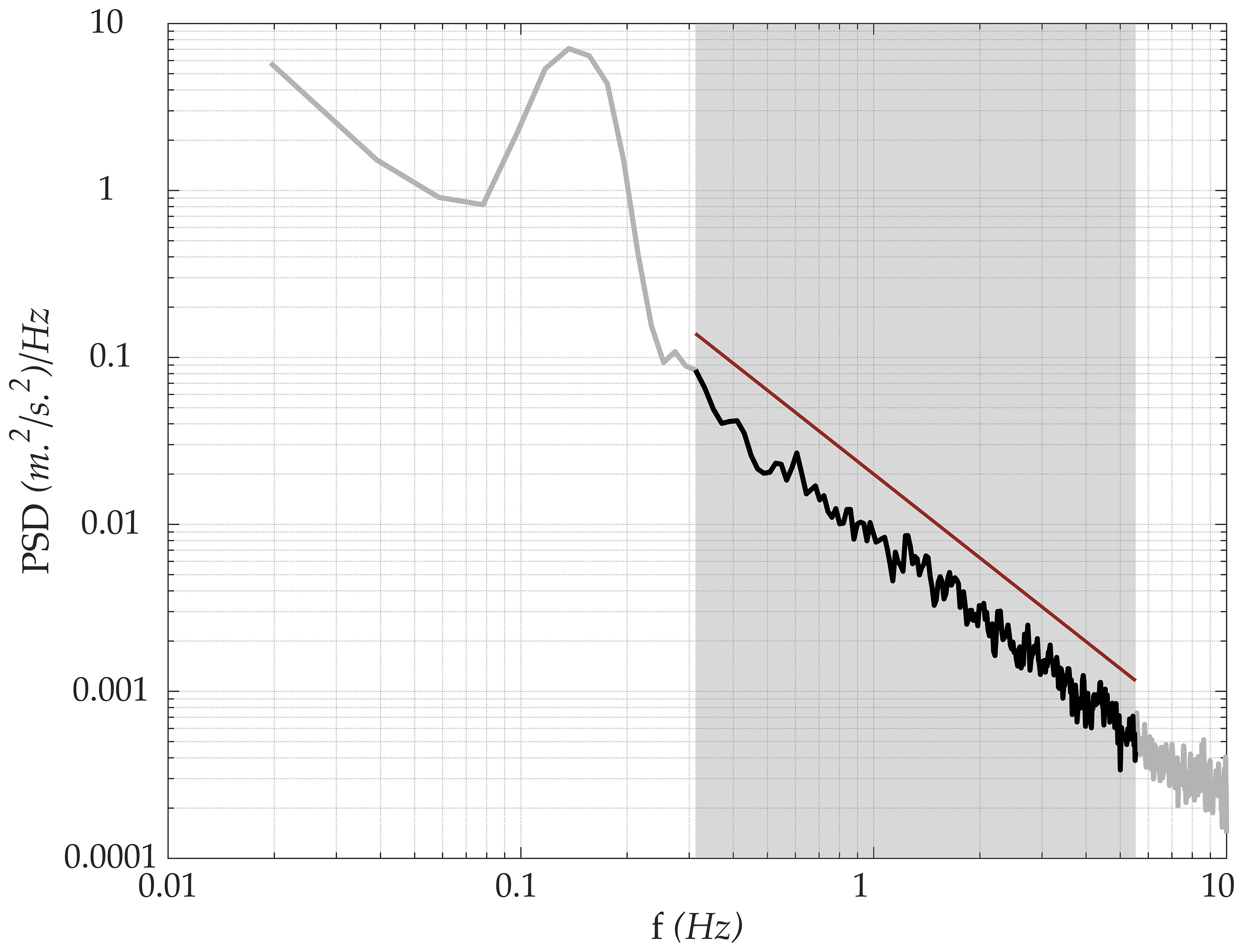
Figure 2. Power spectral density (PSD) of wind speed fluctuations as a function of frequency (f) from a 20-minute data sample. The shaded region highlights the identified inertial subrange, where the PSD aligns with the theoretical f^−5/3 slope, depicted by the solid line.

The assumption of no transport terms in the TKE budget equation (Equation 5) introduces some errors when applied over marine conditions. Consequently, the dissipation rate derived using Equation 6 may be biased if transport terms are not negligible, and this can lead to errors in flux estimation, particularly in non-stationary or rapidly evolving boundary layers.

2.3.3 Bulk methods

The bulk aerodynamical method is the most widely used flux estimation technique in studying the ocean-atmosphere flux transfer. This method uses mean meteorological parameters such as wind speed, air temperature, humidity, and sea surface temperature to indirectly estimate fluxes (Fairall et al., 1996, 2003; Edson et al., 2013) without the need to measure high-frequency turbulence parameters.

The turbulent fluxes of momentum ($\tau$), sensible heat ($H$), and latent heat ($E$) are parameterized in bulk methods using the Monin‐Obukhov similarity theory (MOST) as

$\begin{array}{ll}\tau \approx \rho C_D{U}^2& (7)\end{array}$

$\begin{array}{ll}\text{H}\approx \text{ρ}{C}_p{C}_{H}U({\text{θ}}_s-{\text{θ}}_a)& (8)\end{array}$

$\begin{array}{ll}\text{E}\approx \text{ρ}{L}_e{C}_{E}U(q_s-q_a)& (9)\end{array}$

Where U is the mean wind speed and $C_D$, $C_H$ and $C_E$ the bulk transfer coeficients for stress, sensible heat and latent heat. ${\text{θ}}_a$ is the temperature at reference height while ${\text{θ}}_s$ gives temperature at sea surface. $q_a$ is the specific humidity at reference height and $q_s$ gives saturation specific humidity at the sea surface. In this study, COARE v3.5 algorithm (Edson et al., 2013) wind-speed-dependent formulation is used to estimate turbulent fluxes of heat and momentum (Equations 7–9).

3 EC flux processing algorithm

Accurately calculating wind velocities using the EC method from a moving platform is challenging because the observed wind fluctuations are influenced by platform motion rather than reflecting the true wind. These motion-induced effects come from three main sources: 1) Anemometer tilt: Variations in the platform’s pitch, roll, and heading cause the anemometer to tilt, distorting measurements. 2) Rotational motion: The platform’s rotation about its local axes introduces angular velocity at the anemometer and 3) Translational motion: Linear movements of the platform relative to a fixed reference frame further distort the observed wind velocities. Correcting for this motion-induced contamination is essential for accurate flux calculations. These issues have been extensively documented in earlier studies (e.g., Fujitani, 1981; Anctil et al., 1994; Edson et al., 1998; Miller et al., 2008). Building on the framework from Edson et al. (1998), we calculate the true wind vector, free from motion contamination, in the fixed Earth reference frame as follows:

$\begin{array}{ll}\overrightarrow{V_{True}}=T\overrightarrow{V_{Obs}}+\overrightarrow{\text{Ω}}\times T\overrightarrow{M}+\overrightarrow{V_{Cm}}& (10)\end{array}$

where, $\overrightarrow{V_{True}}$ represents the true wind velocity in the reference coordinates and $\overrightarrow{V_{Obs}}$ is the observed wind vector in the ship’s moving frame. Here, the coordinate transformation matrix $T$ is used to rotate ship coordinates to the reference coordinates. Angular velocity of ship coordinates is denoted as $\overrightarrow{\Omega }$ and $\overrightarrow{M}$ is the position vector of the wind sensor with respect to the IMU. The final term, $\overrightarrow{V_{Cm}}$ accounts for the translational velocity vector at the center of motion of the ship with respect to reference coordinates. The orientation of the sonic anemometer in the fixed frame is defined using three rotational angles obtained from IMU: yaw ($\psi$), pitch ($\theta$), and roll ($\varphi$). $\psi$ represents the rotation about the Z-axis and is positive in the counterclockwise direction. $\theta$ corresponds to the rotation about the intermediate Y-axis and is positive when the ship bow tilts downward. $\varphi$ describes the rotation about the intermediate X-axis and is positive when the port side of the instrument tilts upward. We define coordinate transformation matrix $T$ using these angles as

$\begin{array}{ll}\begin{array}{l}T(\varphi ,\theta ,\psi )=A(\psi )A(\theta )A(\varphi )\\ =\left[\begin{array}{ccc}cos(\psi )& -sin(\psi )& 0\\ sin(\psi )& cos(\psi )& 0\\ 0& 0& 1\end{array}\right]\left[\begin{array}{ccc}cos(\theta )& 0& sin(\theta )\\ 0& 1& 0\\ -sin(\theta )& 0& cos(\theta )\end{array}\right]\left[\begin{array}{ccc}1& 0& 0\\ 0& cos(\varphi )& -sin(\varphi )\\ 0& sin(\varphi )& cos(\varphi )\end{array}\right]\end{array}& (11)\end{array}$

Equation 11 represents the transformation of the coordinate matrix resulting from the combination of three rotations applied to the ship-based coordinate frame. These rotations occur around the three axes of our reference frame (Earth). The rotation order follows a 321 sequence (ZYX axes) following Edson et al. (1998), effectively reducing errors related to the rotation order. The IMU is mounted underneath the sonic anemometer and measures angular rotation about the 3-axis in the ship-based frame. This vector is rotated to fixed frame using $T$ as

$\begin{array}{ll}\overrightarrow{\Omega }=T\overrightarrow{{\text{Ω}}_{Obs}}& (12)\end{array}$

Combining Equations 10 and 12 allows us to rewrite Equation 10 as

$\begin{array}{ll}\overrightarrow{V_{True}}=T( \overrightarrow{V_{Obs}}+\overrightarrow{\Omega }\times \overrightarrow{M})+\overrightarrow{V_{mot}}& (13)\end{array}$

This motion correction approach ensures that the observed winds are adjusted for platform motion, allowing for precise determination of the true wind velocities in the fixed reference frame. Euler angles are estimated by integrating the rate of change of Euler angles in fixed frame obtained from Equation 13 given by

$\begin{array}{ll}\left[\begin{array}{c}\dot{\text{ϕ}}\\ \dot{\text{θ}}\\ \dot{\text{ψ}}\end{array}\right]=\left[\begin{array}{ccc}1& \sin \text{ϕ}\tan \text{θ}& \cos \text{ϕ}\tan \text{θ}\\ 0& \cos \text{ϕ}& \sin \text{ϕ}\\ 0& \sec \text{θ}\sin \text{ϕ}& \sec \text{θ}\cos \text{ϕ}\end{array}\right]\left[\begin{array}{c}\stackrel{}{{\dot{\text{ϕ}}}_{\text{obs}}}\\ \stackrel{}{{\dot{\text{θ}}}_{\text{obs}}}\\ \stackrel{{\dot{\text{ψ}}}_{\text{obs}}}{}\end{array}\right]& (14)\end{array}$

To avoid errors arising from drift in angular sensors, a complementary filtering approach is followed. The angles obtained by applying a high-pass filter to the angles derived from integrating Equation 14 is added with the initial Euler matrix which is approximated using the slow roll, pitch, and yaw angles obtained from the linear accelerometers. A detailed explanation of this method can be found in Edson et al. (1998) and the workflow chart is given by Figure 3.

Figure 3

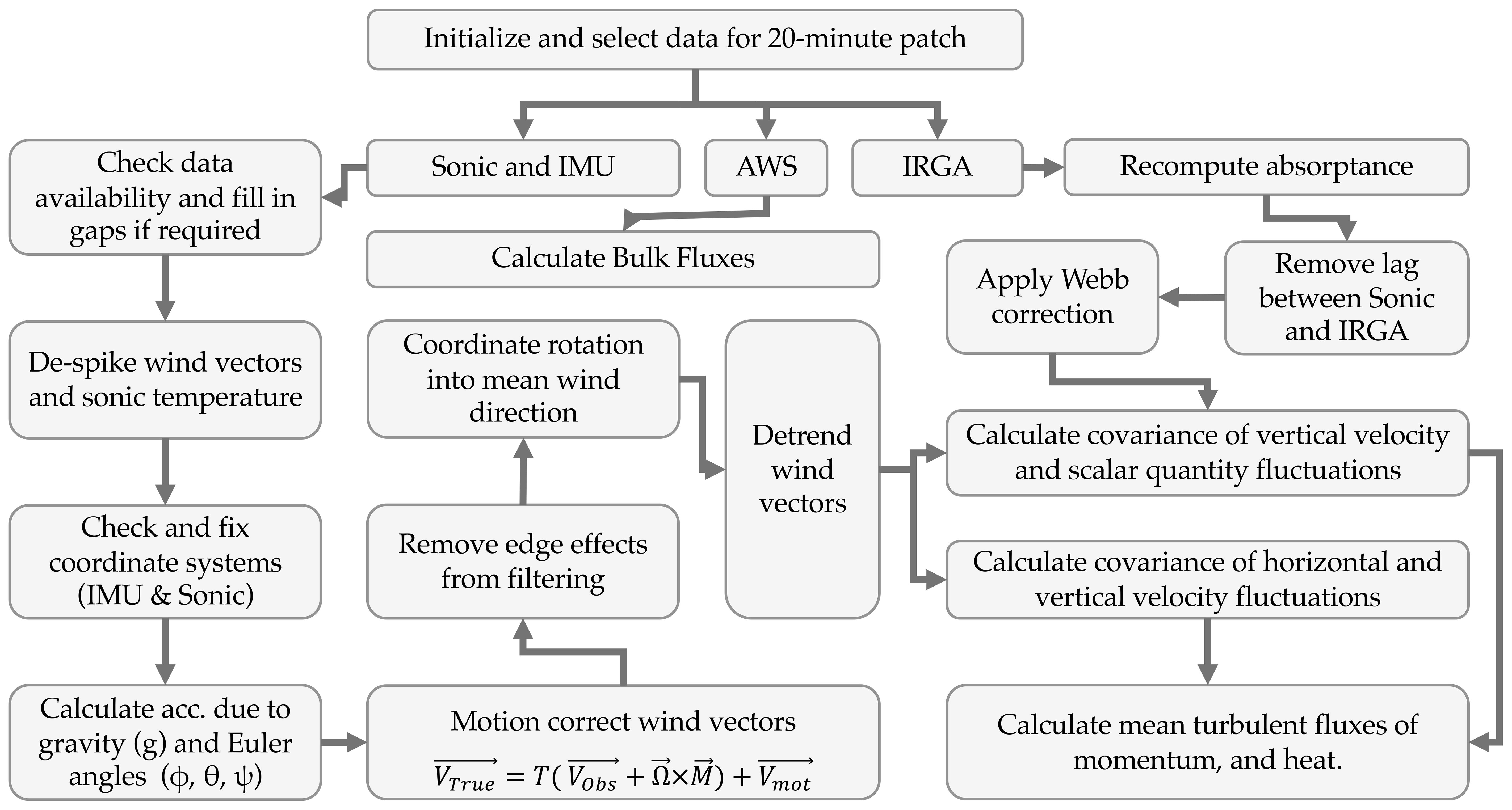
Figure 3. Flowchart with ECFS-FRS workflow, detailing each step of the data processing procedure.

4 Preliminary results

This section presents preliminary results inferred from data collected over the Arabian Sea from July 1 to July 16, 2023, when the relative angle between wind and ship heading was minimal. Figure 4 shows the ship track and wind vectors from measurements onboard. The thick line along the ship track is when the mean relative wind direction was limited to $\pm 60°$ from the bow. The mean wind vectors from ERA-5 reanalysis data product during the cruise period are also included as grey arrows.

Figure 4

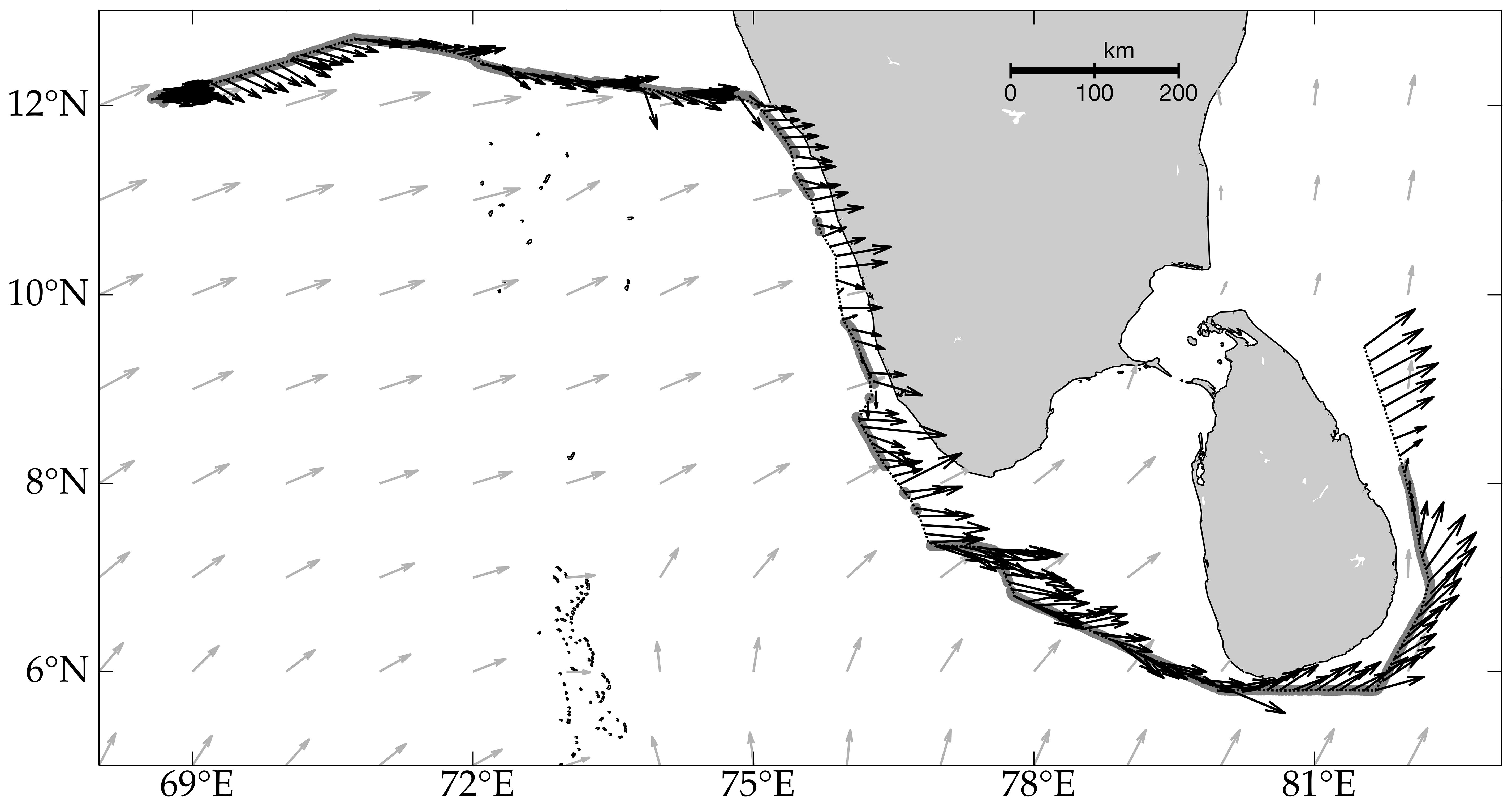
Figure 4. Cruise track of ORV Sagar Nidhi with wind vector recorded by ECFS-FRS, with regions where the ship headed into the wind highlighted by thick grey lines. The vectors (grey) in the map shows mean wind vectors from ERA5 reanalysis data during observation period.

4.1 Met-ocean weather conditions during July 2023

The AWS time-series observations in Figure 5 provide insights into the met-ocean weather conditions that prevailed during the cruise period. Initially, from the start of the cruise until July 7, wind speeds ranged between 10–15 m/s (Figure 5a). This period was characterized by frequent episodes of rain (Figure 5f) and a notable decrease in both SST_skin (Figure 5d) and near-surface air temperature (Figure 5e). Concurrently, relative humidity remained consistently high, fluctuating between 80-90% throughout the entire duration (Figure 5c). The persistent cloud cover obstructed the incoming shortwave radiation, and also increased the reflected downwelling longwave radiation. The wind direction remained predominantly easterly during this period. Between July 7 and 9, ORV Sagar Nidhi traversed through a strong SST front, witnessing a remarkable 3°C jump in SST_skin from 25.5°C to 28.5°C. In the rest of the period, SST_skin and air temperatures remained above 28°C, and rainfall became sporadic. Clear skies prevailed, facilitating increased incoming shortwave radiation, and surface winds ranged between 8–10 m/s.

4.2 Friction velocity comparison between EC, IDM and bulk

In this section, we compare the friction velocity (${\text{U}}_{*}$) timeseries instead of wind stress as ${\text{U}}_{*}$ directly represents momentum transfer and is a common parameter across all flux estimation methods, making it ideal for consistent comparison. Also, unlike wind stress, ${\text{U}}_{*}$ is independent of air density variations and avoids additional uncertainties introduced by assumptions like drag coefficients. We estimated ${\text{U}}_{*}$ using three widely recognized methods described in Section 2.3: the Eddy Covariance (EC) method, the Inertial Dissipation Method (IDM), and the Bulk Method (BK). Each method has distinct advantages and limitations, requiring careful consideration of their applicability and constraints.

Figure 5

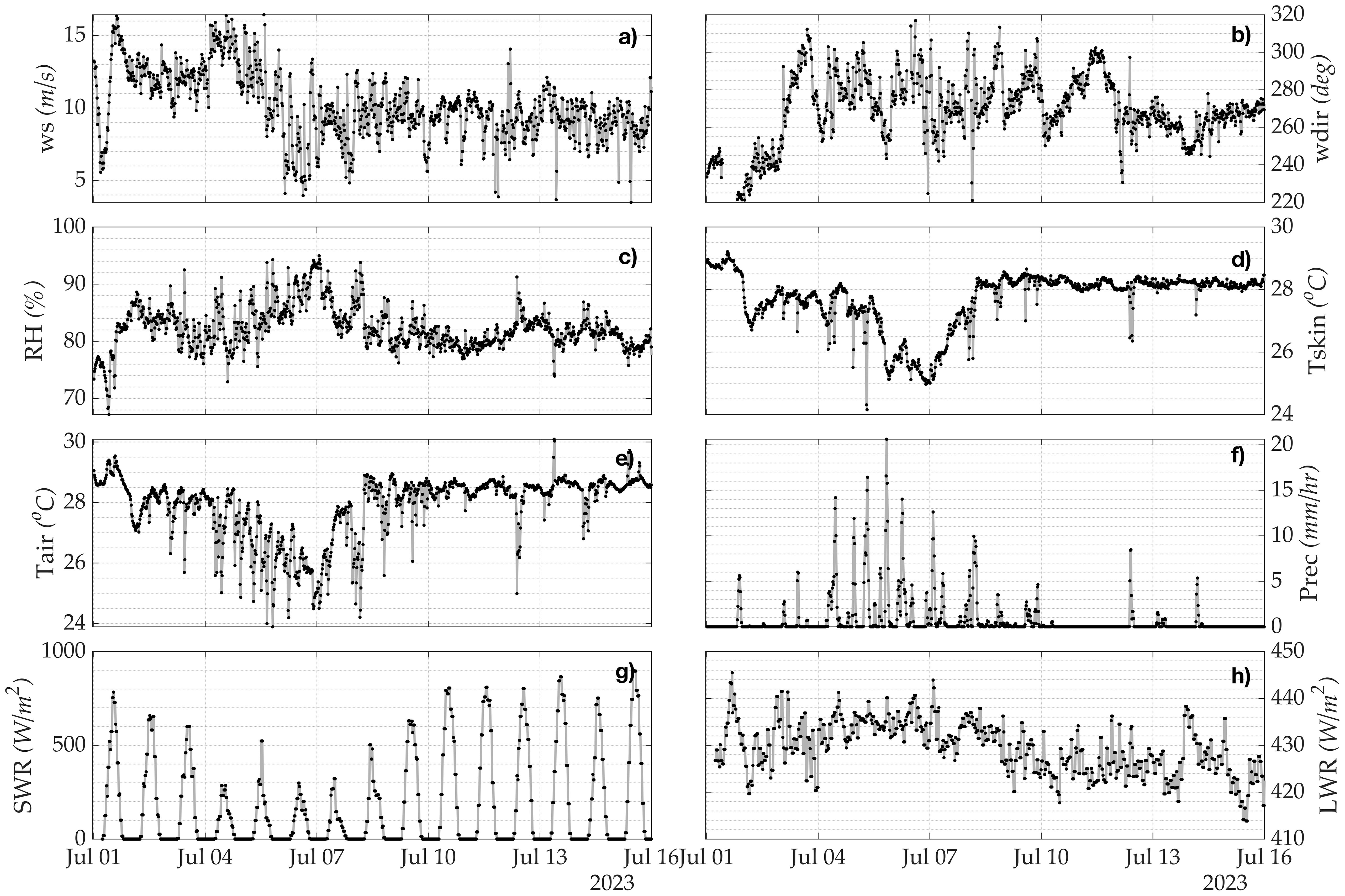
Figure 5. Time series of met-ocean parameters recorded by INCOIS-FRS, including (a) wind speed, (b) wind direction, (c) relative humidity (RH), (d) skin sea surface temperature (SST), (e) air temperature, (f) precipitation, (g) shortwave radiation (SWR), and (h) longwave radiation (LWR).

The time series of ${\text{U}}_{*}$ from these methods is presented in Figure 6. Generally, the bulk-derived ${\text{U}}_{*}$ values underestimated those from the EC method. On a daily scale, the bulk and EC estimates showed a correlation of 0.51 with an RMS error of 0.11. During the analysis period, stable boundary layer conditions (z/L>0) prevailed from July 2 to July 4, transitioning to unstable conditions (z/L<0) from July 4 onward. Under unstable conditions, the bulk method significantly underestimated ${\text{U}}_{*}$ compared to EC values, highlighting the need to revisit flux-profile parameterizations for stable and unstable conditions specific to the Arabian Sea.

Figure 6

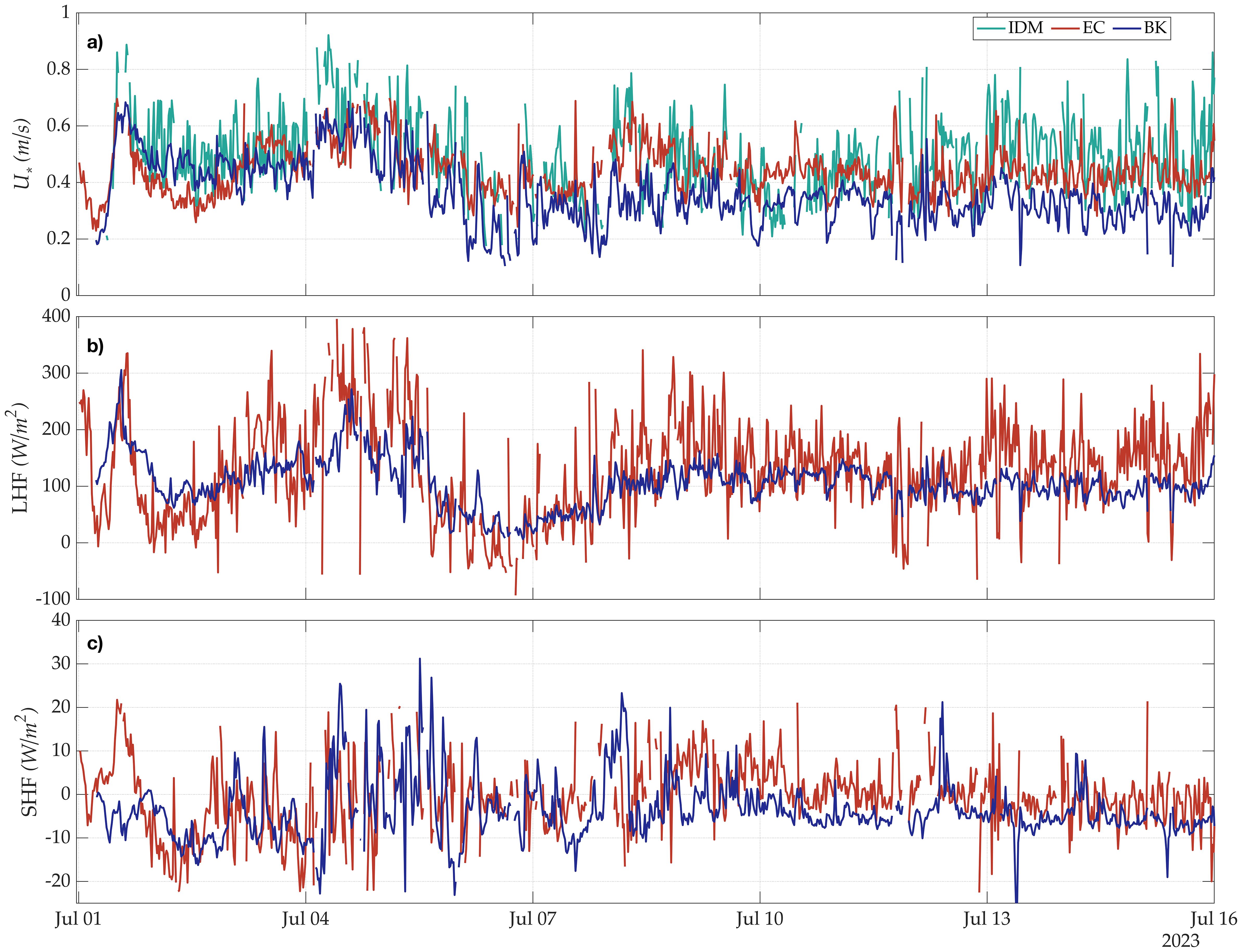
Figure 6. (a) Friction velocity (U*) comparison from EC, IDM and BK, (b) Sensible and (c) Latent Heat flux from EC and BK.

Conversely, the IDM-derived ${\text{U}}_{*}$consistently overestimated EC values. The IDM estimates wind stress transferred from the atmosphere to the ocean. However, during swell-dominated conditions, reverse stress transfer from swells to the atmosphere reduces the net stress imparted by wind on the sea. Chen et al. (2020) demonstrated that the influence of swells on wind stress can be felt as high as 17 m above the sea surface, indicating that our observational records also might as well capture the impact of swells. While the EC method captures this bidirectional stress interaction, IDM does not, leading to a positive bias in IDM-derived ${\text{U}}_{*}$. This bias is often addressed by including an imbalance term in the TKE budget equation. For example, Bourras et al. (2019) suggested an optimal imbalance term of 0.4, while Cambra (2015) proposed 0.5. However, a region-specific value for the Arabian Sea needs to be determined to improve the accuracy of IDM-derived ${\text{U}}_{*}$ under swell-dominated conditions.

4.3 Sensible and latent heat flux comparison between EC and bulk

Studies have shown that wind stress comparisons between EC and IDM methods agree within 20%, while large uncertainty exists between their LHF and SHF estimations (Fairall et al., 1990; Edson et al., 1991). In order to check it, this section presents the time series of bulk versus EC LHF and SHF, respectively (Figures 6b, c). At daily timescales, the LHF comparison yields a correlation coefficient of 0.8 and an RMS error of 45 W/m², while SHF shows r = 0.63 and an RMS error of 4.2 W/m², indicating a reasonably good agreement between the bulk and EC methods. However, bulk-derived LHF and SHF consistently underestimate their EC counterparts, with mean biases of -26 W/m² for LHF and -3 W/m² for SHF, resulting in large rms errors, highlighting systematic discrepancies in the bulk estimates.

These discrepancies arise from several factors, which need to be further analyzed. Simplified parameterizations in bulk algorithms can inadequately represent complex surface-layer physics. Stability effects can lead to significant deviations from true flux values, particularly during unstable conditions (Srivastava and Sharan, 2021). Additionally, swell-induced modifications of the roughness layer can alter surface dynamics, introducing further uncertainties (Raj et al., 2024). Errors in converting bulk SST to skin SST also contribute to inaccuracies, as bulk SST fails to account for critical surface-layer processes like the cool-skin effect and diurnal warming (Murray et al., 2000; Alappattu et al., 2017). These combined factors distort the air-sea temperature gradient, a key driver of both evaporation and heat transfer, leading to systematic underestimations in bulk-derived LHF and SHF.

The integration of a skin SST-measuring radiometer into the INCOIS-FRS onboard ORV Sagar Nidhi marks a major step forward in addressing these challenges. $SS{T}_{skin}$ offers a precise representation of the ocean’s surface temperature, accurately capturing processes such as nighttime cooling by the cool-skin layer and daytime diurnal warming. By using this data, bulk flux estimates can be refined to better reflect true air-sea flux dynamics. With sufficient data collected by INCOIS-FRS, future efforts should thoroughly verify and refine bulk-to-skin SST conversion algorithms, ensuring enhanced reliability in both LHF and SHF estimates.

With sufficient data collection over time, this system has the potential to play a pivotal role in refining bulk-to-skin SST algorithms. Future efforts should focus on thoroughly verifying these algorithms using the high-resolution skin SST data from INCOIS-FRS, paving way for more accurate parameterizations of bulk heat flux. This development is particularly important for regions like the Arabian Sea, where significant diurnal and seasonal variations in surface thermal structure exist.

5 Concluding remarks

This article introduces the INCOIS Flux Reference System (INCOIS-FRS), developed and installed aboard the ORV Sagar Nidhi by the Indian National Centre for Ocean Information Services (INCOIS). The INCOIS-FRS is an integrated system designed to precisely measure air-sea fluxes along the ship’s track. It comprises two key components: the Eddy Covariance Flux System (ECFS) and the Automated Weather Station (AWS). The ECFS, equipped with a 3-axis sonic anemometer, an infrared gas analyzer (IRGA), and an inertial motion unit (IMU), captures critical parameters such as wind components, temperature, gas concentrations, and platform motion, providing high-frequency data (20 Hz) to estimate momentum, heat, and gas fluxes. Complementing this, the AWS records mean meteorological variables at 1Hz, including wind speed and direction, air temperature, relative humidity, barometric pressure, and precipitation. It also includes an infrared radiometer for skin sea surface temperature ($SS{T}_{skin}$) measurements, providing a comprehensive set of data for detailed flux analysis.

This paper details the EC data processing steps for post-processing INCOIS-FRS data and presents preliminary results from the Arabian Sea during the summer monsoon of 2023. Despite the limited dataset, the findings underscore the potential of INCOIS-FRS for fine-scale micrometeorological studies and advancing our understanding of air-sea interactions and flux transfer processes. Initial analysis reveals significant discrepancies between bulk flux parameterizations of latent and sensible heat fluxes and the reference fluxes obtained using the Eddy Covariance (EC) method. Additionally, friction velocity estimates from the Inertial Dissipation Method (IDM) show notable deviations from EC measurements. These results highlight the critical need for validating bulk flux parameterizations using Indian Ocean-specific datasets.

Existing flux transfer parameterizations require significant refinement, particularly in accounting for Indian Ocean conditions. Previous studies have shown that wind and stress vectors often misalign, challenging the assumptions of Monin-Obukhov Similarity Theory (MOST) and leading to deviations in wind stress magnitude and direction (Raj et al., 2024). The INCOIS-FRS offers an ideal platform to explore such misalignments and refine transfer coefficient calculations. Another crucial consideration is the conversion of bulk SST to skin SST in bulk flux algorithms like COARE. Studies like Liu et al. (2023) emphasize the need to integrate boundary-layer processes to simulate accurately $SS{T}_{skin}$ under varying wind and atmospheric stability conditions. INCOIS-FRS provides an excellent platform to test these models.

The INCOIS-FRS represents a major step forward in collecting fine-scale, direct flux measurement data from the marine environment around the Indian Ocean. Its deployment marks the beginning of other broader efforts to equip more crewed and uncrewed platforms with similar systems. With continued data collection and advancements in observational platforms, INCOIS-FRS will play a critical role in enhancing the accuracy of air-sea flux estimates and enabling improvements in climate and oceanic models, ultimately contributing to a deeper understanding of the coupled ocean-atmosphere system.

Data availability statement

The original contributions presented in the study are included in the article/supplementary material. Further inquiries can be directed to the corresponding author. Data related enquiries can be directed to the corresponding author.

Author contributions

BK: Conceptualization, Formal Analysis, Funding acquisition, Investigation, Methodology, Project administration, Resources, Supervision, Writing – original draft, Writing – review & editing. AR: Data curation, Methodology, Software, Visualization, Writing – review & editing. AS: Data curation, Software, Visualization, Writing – review & editing. NS: Data curation, Resources, Writing – review & editing. AG: Resources, Writing – review & editing. DS: Resources, Writing – review & editing. KR: Resources, Writing – review & editing. VJ: Data curation, Methodology, Resources, Writing – review & editing. ER: Funding acquisition, Resources, Writing – review & editing.

Funding

The author(s) declare that financial support was received for the research and/or publication of this article. Ministry of Earth Sciences (MoES), Govt. of India provided the necessary fundingto carry out this research.

Acknowledgments

The authors gratefully acknowledge Director, INCOIS for facilitating this research. Special thanks to Mr. Nageswara Rao, Mr. Devendrakumar, and Mr. Subramanyam from the INCOIS administration for their invaluable support in ensuring the smooth purchase and installation of the INCOIS-FRS components. We also extend our appreciation to the Vessel Management Cell (VMC) of NIOT for their continued support. We are especially thankful to M/s Tridel Technologies for providing technical expertise in installing the system. Dr. Girishkumar, Chief Scientist of ORV Sagar Nidhi cruise in July 2023, its Captain and crew are thanked for facilitating data collection. This article bears INCOIS contribution number 564.

Conflict of interest

The authors declare that the research was conducted in the absence of any commercial or financial relationships that could be construed as a potential conflict of interest.

Generative AI statement

The author(s) declare that no Generative AI was used in the creation of this manuscript.

Publisher’s note

All claims expressed in this article are solely those of the authors and do not necessarily represent those of their affiliated organizations, or those of the publisher, the editors and the reviewers. Any product that may be evaluated in this article, or claim that may be made by its manufacturer, is not guaranteed or endorsed by the publisher.

References

Alappattu D. P., Wang Q., Yamaguchi R., Lind R. J., Reynolds M., and Christman A. J. (2017). Warm layer and cool skin corrections for bulk water temperature measurements for air-sea interaction studies. J. Geophys. Res. Oceans 122, 6470–6481. doi: 10.1002/2017JC012688

Crossref Full Text | Google Scholar

Anctil F., Donelan M. A., Drennan W. M., and Graber H. C. (1994). Eddy-correlation measurements of air-sea fluxes from a discus buoy. J. Atmospheric Ocean. Technol. 11, 1144–1150. doi: 10.1175/1520-0426(1994)011<1144:ECMOAS>2.0.CO;2

Crossref Full Text | Google Scholar

Anderson R. J. (1993). A study of wind stress and heat flux over the open ocean by the inertial-dissipation method. J. Phys. Oceanogr. 23, 2153–2161. doi: 10.1175/1520-0485(1993)023<2153:ASOWSA>2.0.CO;2

Crossref Full Text | Google Scholar

Bhat G. S. (2003). Measurement of air–sea fluxes over the indian ocean and the bay of bengal. J. Clim. 16, 767–775. doi: 10.1175/1520-0442(2003)016<0767:MOASFO>2.0.CO;2

Crossref Full Text | Google Scholar

Bourlès B., Lumpkin R., McPhaden M. J., Hernandez F., Nobre P., Campos E., et al. (2008). THE PIRATA PROGRAM: History, accomplishments, and future directions. Bull. Am. Meteorol. Soc 89, 1111–1126. doi: 10.1175/2008BAMS2462.1

Crossref Full Text | Google Scholar

Bourras D., Cambra R., Marié L., Bouin M., Baggio L., Branger H., et al. (2019). Air-sea turbulent fluxes from a wave-following platform during six experiments at sea. J. Geophys. Res. Oceans 124, 4290–4321. doi: 10.1029/2018JC014803

Crossref Full Text | Google Scholar

Cambra R. (2015) Etude des flux turbulents à l’interface air-mer à partir de données de la plateforme OCARINA. Available online at: http://www.theses.fr/2015SACLV024/document.

Google Scholar

Carton J. A., Chepurin G. A., and Chen L. (2018). SODA3: A new ocean climate reanalysis. J. Clim. 31, 6967–6983. doi: 10.1175/JCLI-D-18-0149.1

Crossref Full Text | Google Scholar

Champagne F. H., Friehe C. A., LaRue J. C., and Wynagaard J. C. (1977). Flux measurements, flux estimation techniques, and fine-scale turbulence measurements in the unstable surface layer over land. J. Atmospheric Sci. 34, 515–530. doi: 10.1175/1520-0469(1977)034<0515:FMFETA>2.0.CO;2

Crossref Full Text | Google Scholar

Chen S., Qiao F., Jiang W., Guo J., and Dai D. (2019). Impact of surface waves on wind stress under low to moderate wind conditions. J. Phys. Oceanogr. 49, 2017–2028. doi: 10.1175/JPO-D-18-0266.1

Crossref Full Text | Google Scholar

Chen S., Qiao F., Xue Y., Chen S., and Ma H. (2020). Directional characteristic of wind stress vector under swell-dominated conditions. J. Geophys. Res. Oceans 125, e2020JC016352. doi: 10.1029/2020JC016352

Crossref Full Text | Google Scholar

Cronin M. F., Gentemann C. L., Edson J., Ueki I., Bourassa M., Brown S., et al. (2019). Air-sea fluxes with a focus on heat and momentum. Front. Mar. Sci. 6, 430. doi: 10.3389/fmars.2019.00430

Crossref Full Text | Google Scholar

Drennan W. M., Graber H. C., Hauser D., and Quentin C. (2003). On the wave age dependence of wind stress over pure wind seas. J. Geophys. Res. Oceans 108, 2000JC000715. doi: 10.1029/2000JC000715

Crossref Full Text | Google Scholar

Edson J. B., Fairall C. W., Mestayer P. G., and Larsen S. E. (1991). A study of the inertial-dissipation method for computing air-sea fluxes. J. Geophys. Res. Oceans 96, 10689–10711. doi: 10.1029/91JC00886

Crossref Full Text | Google Scholar

Edson J. B., Hinton A. A., Prada K. E., Hare J. E., and Fairall C. W. (1998). Direct covariance flux estimates from mobile platforms at sea*. J. Atmospheric Ocean. Technol. 15, 547–562. doi: 10.1175/1520-0426(1998)015<0547:DCFEFM>2.0.CO;2

Crossref Full Text | Google Scholar

Edson J. B., Jampana V., Weller R. A., Bigorre S. P., Plueddemann A. J., Fairall C. W., et al. (2013). On the exchange of momentum over the open ocean. J. Phys. Oceanogr. 43, 1589–1610. doi: 10.1175/JPO-D-12-0173.1

Crossref Full Text | Google Scholar

Fairall C. W., Bradley E. F., Hare J. E., Grachev A. A., and Edson J. B. (2003). Bulk parameterization of air–sea fluxes: Updates and verification for the COARE algorithm. J. Clim. 16, 571–591. doi: 10.1175/1520-0442(2003)016<0571:BPOASF>2.0.CO;2

Crossref Full Text | Google Scholar

Fairall C. W., Bradley E. F., Rogers D. P., Edson J. B., and Young G. S. (1996). Bulk parameterization of air-sea fluxes for Tropical Ocean-Global Atmosphere Coupled-Ocean Atmosphere Response Experiment. J. Geophys. Res. Oceans 101, 3747–3764. doi: 10.1029/95JC03205

Crossref Full Text | Google Scholar

Fairall C. W., Edson J. B., Larsen S. E., and Mestayer P. G. (1990). Inertial-dissipation air-sea flux measurements: A prototype system using realtime spectral computations. J. Atmospheric Ocean. Technol. 7, 425–453. doi: 10.1175/1520-0426(1990)007<0425:IDASFM>2.0.CO;2

Crossref Full Text | Google Scholar

Fujitani T. (1981). Direct measurement of turbulent fluxes over the sea during AMTEX. Pap. Meteorol. Geophys. 32, 119–134. doi: 10.2467/mripapers.32.119

Crossref Full Text | Google Scholar

Garbe C. S., Rutgersson A., Boutin J., De Leeuw G., Delille B., Fairall C. W., et al. (2014). “Transfer across the air-sea interface,” in Ocean-atmosphere interactions of gases and particles. Eds. Liss P. S. and Johnson M. T. (Berlin, Heidelberg: Springer Berlin Heidelberg), 55–112. doi: 10.1007/978-3-642-25643-1_2

Crossref Full Text | Google Scholar

Hackerott J. A., Pezzi L. P., Bakhoday Paskyabi M., Oliveira A. P., Reuder J., De Souza R. B., et al. (2018). The role of roughness and stability on the momentum flux in the marine atmospheric surface layer: A study on the southwestern atlantic ocean. J. Geophys. Res. Atmospheres 123, 3914–3932. doi: 10.1002/2017JD027994

Crossref Full Text | Google Scholar

Hakuba M. Z., Fourest S., Boyer T., Meyssignac B., Carton J. A., Forget G., et al. (2024). Trends and variability in earth’s energy imbalance and ocean heat uptake since 2005. Surv. Geophys. 45, 1721–1756. doi: 10.1007/s10712-024-09849-5

Crossref Full Text | Google Scholar

Hicks B. B. and Dyer A. J. (1972). The spectral density technique for the determination of eddy fluxes. Q. J. R. Meteorol. Soc 98, 838–844. doi: 10.1002/qj.49709841810

Crossref Full Text | Google Scholar

Kato S., Loeb N. G., Rose F. G., Doelling D. R., Rutan D. A., Caldwell T. E., et al. (2013). Surface irradiances consistent with CERES-derived top-of-Atmosphere shortwave and longwave irradiances. J. Clim. 26, 2719–2740. doi: 10.1175/JCLI-D-12-00436.1

Crossref Full Text | Google Scholar

Large W. G. and Pond S. (1981). Open ocean momentum flux measurements in moderate to strong winds. J. Phys. Oceanogr. 11, 324–336. doi: 10.1175/1520-0485(1981)011<0324:OOMFMI>2.0.CO;2

Crossref Full Text | Google Scholar

Liu Z., Yang M., Qu L., and Guan L. (2023). Regional study on the oceanic cool skin and diurnal warming effects: Observing and modeling. Remote Sens. 15, 3814. doi: 10.3390/rs15153814

Crossref Full Text | Google Scholar

Martin M. J., Hines A., and Bell M. J. (2007). Data assimilation in the FOAM operational short-range ocean forecasting system: a description of the scheme and its impact. Q. J. R. Meteorol. Soc 133, 981–995. doi: 10.1002/qj.74

Crossref Full Text | Google Scholar

Mcbean G. A. and Elliott J. A. (1975). The vertical transports of kinetic energy by turbulence and pressure in the boundary layer. J. Atmospheric Sci. 32, 753–766. doi: 10.1175/1520-0469(1975)032<0753:TVTOKE>2.0.CO;2

Crossref Full Text | Google Scholar

McPhaden M. J., Busalacchi A. J., Cheney R., Donguy J., Gage K. S., Halpern D., et al. (1998). The tropical ocean-global atmosphere observing system: A decade of progress. J. Geophys. Res. Oceans 103, 14169–14240. doi: 10.1029/97JC02906

Crossref Full Text | Google Scholar

McPhaden M. J., Connell K., Foltz G., Perez R., and and Grissom K. (2023). Tropical ocean observations for weather and climate: A decadal overview of the global tropical moored buoy array. Oceanography. doi: 10.5670/oceanog.2023.211

Crossref Full Text | Google Scholar

McPhaden M. J., Ando K., Bourlès B., Freitag H. P., Lumpkin R., Masumoto Y., et al. (2010). “The global tropical moored buoy array,” in Proceedings of OceanObs’09: Sustained ocean observations and information for society (European Space Agency), 668–682. doi: 10.5270/OceanObs09.cwp.61

Crossref Full Text | Google Scholar

McPhaden M. J., Meyers G., Ando K., Masumoto Y., Murty V. S. N., Ravichandran M., et al. (2009). RAMA: The research moored array for african–Asian–Australian monsoon analysis and prediction*. Bull. Am. Meteorol. Soc 90, 459–480. doi: 10.1175/2008BAMS2608.1

Crossref Full Text | Google Scholar

Miller S. D., Hristov T. S., Edson J. B., and Friehe C. A. (2008). Platform motion effects on measurements of turbulence and air–sea exchange over the open ocean. J. Atmospheric Ocean. Technol. 25, 1683–1694. doi: 10.1175/2008JTECHO547.1

Crossref Full Text | Google Scholar

Murray M. J., Allen M. R., Merchant C. J., Harris A. R., and Donlon C. J. (2000). Direct observations of skin-bulk SST variability. Geophys. Res. Lett. 27, 1171–1174. doi: 10.1029/1999GL011133

Crossref Full Text | Google Scholar

Oost W. A., Komen G. J., Jacobs C. M. J., and Van Oort C. (2002). New evidence for a relation between wind stress and wave age from measurements during ASGAMAGE. Bound.-Layer Meteorol. 103, 409–438. doi: 10.1023/A:1014913624535

Crossref Full Text | Google Scholar

Pezzi L. P., Souza R. B., Farias P. C., Acevedo O., and Miller A. J. (2016). Air-sea interaction at the s outhern b razilian c ontinental s helf: In situ observations. J. Geophys. Res. Oceans 121, 6671–6695. doi: 10.1002/2016JC011774

Crossref Full Text | Google Scholar

Pond S., Phelps G. T., Paquin J. E., McBean G., and Stewart R. W. (1971). Measurements of the turbulent fluxes of momentum, moisture and sensible heat over the ocean. J. Atmospheric Sci. 28, 901–917. doi: 10.1175/1520-0469(1971)028<0901:MOTTFO>2.0.CO;2

Crossref Full Text | Google Scholar

Raj A., Praveen Kumar B., Jampana V., Shivaprasad S., Sureshkumar N., Rao E. P. R., et al. (2024). Turbulent characteristics of momentum flux in the marine atmospheric boundary layer of north bay of bengal. Sci. Rep. 14, 22073. doi: 10.1038/s41598-024-71819-z

PubMed Abstract | Crossref Full Text | Google Scholar

Santini M. F., Souza R. B., Pezzi L. P., and Swart S. (2020). Observations of air–sea heat fluxes in the southwestern atlantic under high-frequency ocean and atmospheric perturbations. Q. J. R. Meteorol. Soc 146, 4226–4251. doi: 10.1002/qj.3905

Crossref Full Text | Google Scholar

Sauvage C., Seo H., Clayson C. A., and and Edson J. B. (2023). Improving Wave-Based Air-Sea Momentum Flux Parameterization in Mixed Seas. J. Geophys. Res. Oceans 128, e2022JC019277. doi: 10.1029/2022JC019277

Crossref Full Text | Google Scholar

Send U., Weller R. A., Wallace D., Chavez F., Lampitt R., Dickey T., et al. (2010). “OceanSITES,” in Proceedings of oceanObs’09: sustained ocean observations and information for society, (European Space Agency), 854–863. doi: 10.5270/OceanObs09.cwp.79

Crossref Full Text | Google Scholar

Srivastava P. and Sharan M. (2021). Uncertainty in the parameterization of surface fluxes under unstable conditions. J. Atmospheric Sci. doi: 10.1175/JAS-D-20-0350.1

Crossref Full Text | Google Scholar

Storto A., Alvera-Azcárate A., Balmaseda M. A., Barth A., Chevallier M., Counillon F., et al. (2019). Ocean reanalyses: Recent advances and unsolved challenges. Front. Mar. Sci. 6, 418. doi: 10.3389/fmars.2019.00418

Crossref Full Text | Google Scholar

Storto A., Martin M. J., Deremble B., and Masina S. (2018). Strongly coupled data assimilation experiments with linearized ocean–atmosphere balance relationships. Mon. Weather Rev. 146, 1233–1257. doi: 10.1175/MWR-D-17-0222.1

Crossref Full Text | Google Scholar

Valdivieso M., Haines K., Balmaseda M., Chang Y.-S., Drevillon M., Ferry N., et al. (2017). An assessment of air–sea heat fluxes from ocean and coupled reanalyses. Clim. Dyn. 49, 983–1008. doi: 10.1007/s00382-015-2843-3

Crossref Full Text | Google Scholar