Abstract
With the promotion of the “Belt and Road,” the container multimodal transportation between China and Europe has faced unprecedented development opportunities. In view of the increasing concern about carbon emissions and uncertainty during transportation, this paper constructs a robust optimization model with carbon emission constraints and aims at minimizing both the operation cost and operation time. A Nondominated Sorting Genetic Algorithm-II (NSGA-II) is devised to tackle the proposed model. After that, the paper exemplifies the container multimodal transportation from Nanjing, China to Berlin, Germany, conducting an empirical study on optimizing the Eurasian container multimodal transportation plan. A small-scale case compares the results from CPLEX and NSGA-II, validating the effectiveness of the proposed model and algorithm. Then, a comparison is made between the single-objective and multi-objective results. It is demonstrated that multi-objective optimization can resolve conflicts among sub-objectives and derive a compromise solution for multiple objectives. Subsequently, results under different fluctuation scenarios show that the robust model is applicable to all situations. Finally, a sensitivity analysis of the robust model is carried out, considering varying carbon emission limits, operating time windows, and regret values. The proposed model and algorithm can serve as a reliable decision reference for multimodal operators, remaining useful during unexpected incidents.
1 Introduction
Ever since President Xi of China proposed the “One Belt, One Road” Initiative in 2013, the mutual trade between China and Europe has experienced enormous development. According to related statistics (Eurostat, 2024), at the beginning of the proposal in 2013, the two-way trade value between China and the European Union (EU) is 559.01 billion dollars, while that value has reached 740.00 billion dollars in 2023, rising by 32.36%. Therein, the export trade value from China to Europe is 712.27 billion dollars, which is 21.07% of the total export value; the import value from Europe to China is 498.30 billion dollars, which is 19.49% of the total import value (National Bureau of Statistics of China, 2024). As global climate change continues to pose a serious threat, countries around the world are working collaboratively to address the issue of carbon emissions (Xu et al., 2024a). The shipping sector accounts for approximately 3% of global greenhouse gas emissions. While its share is relatively small, its long-term environmental impact cannot be overlooked (Xiao et al., 2025). Reducing carbon emissions has become a central task for nations striving to achieve sustainable development (Xin-gang et al., 2023; Xu et al., 2024b). Shipping companies should step up investment in research and development for carbon emission reduction technologies from a long-term perspective (Xiao and Cui, 2023). The growing demand for trade has created an urgent need for transportation modes that are cost-effective, low-emission, and highly efficient. Container transportation has gradually become a main transportation mode in the China–Europe network. At present, there are three main container transportation corridors between China and Europe. They are (1) the sea transportation corridor; (2) the railway transportation corridor mainly based on the China Railway Express (CRE); and (3) the sea–land express transportation passage via Piraeus mainly based on sea and railway transportation. The operation process based on these three main corridors is shown in Figures 1–3. Each of the transport corridor has its own advantages and disadvantages, while complementing each other (Yang et al., 2018).
Figure 1
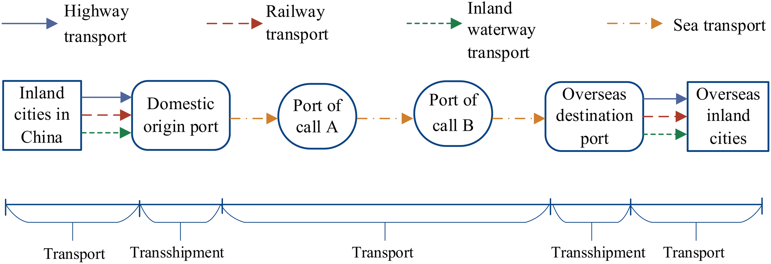
Simplified diagram of the China–Europe sea transport corridor.
Figure 2
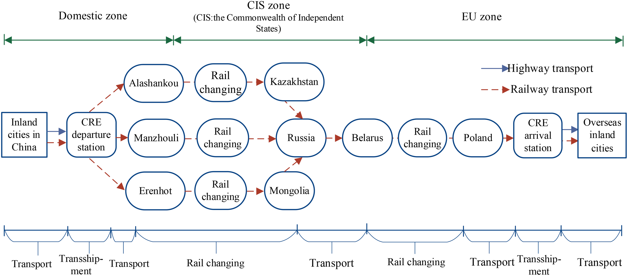
Simplified diagram of the China–Europe railway corridor.
Figure 3
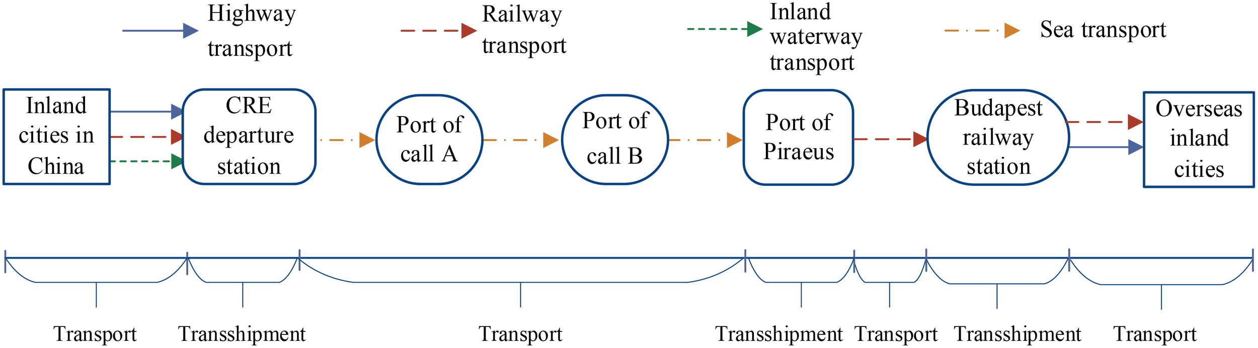
Simplified diagram of the China–Europe sea–land express corridor.
Because of the long distance of container multimodal transport between China and Europe, various modes of transport, and the complicated operation process in many countries, there are many uncertain factors in the operation (Li et al., 2022). For example, road congestion, mechanical failure of vehicles, sudden traffic accidents, or bad weather conditions may result in fluctuations in transport time. Cycles of fuel rates, changes in international situation, and other factors may cause large differences in transport costs in transit. Vehicle congestion in container yards, shortage of handling facilities, and many other factors may lead to the change of the transit time (Im et al., 2021; Cao et al., 2024). Influenced by the uncertain factors mentioned above, the optimized scheme for the container multimodal transportation with different situations might be quite different.
Reasonably choosing the transport route between China and EU under uncertain conditions has great significance. It is critical to reduce operating costs, improve transport efficiency, and provide solid and powerful transport service support for the two-way trade between China and EU. In addition, considering the impact of carbon emission restrictions on the transportation scheme can urge decision-makers to plan transportation routes from the perspective of environmental sustainability and provide decision-making reference for policymakers (Shen et al., 2022). Based on the analysis above, this paper will investigate the routing optimization problem of the Eurasian container multimodal transport system considering uncertain transportation cost, transportation time, and transshipment time. We will establish the robust optimization model for the problem and design the Nondominated Sorting Genetic Algorithm-II (NSGA-II) to solve the model according to the characteristics of the problem. Then, the effectiveness of the model and algorithm is verified by empirical research.
The rest of the paper is organized as follows. Section 2 includes the literature review, from the perspective of the Eurasian transportation corridor and the multimodal routing optimization. Section 3 involves the establishment of the multi-objective robust optimization model. Section 4 proposes the NSGA-II considering the characteristics of the problem. Section 5 is the empirical study considering the container transport between Nanjing and Berlin. Section 6 comprises the conclusion and future research direction.
2 Literature review
2.1 Research about the Eurasian transport corridor
Research on the Eurasian transport corridor mainly focuses on CRE, sea transportation, and Eurasian sea rail combined transportation, among which the research on CRE is the main topic.
As to the research about CRE, Guo et al. (2024a) proposed a novel two-stage transfer learning model named T.R2_LSTM_A. It significantly enhances the accuracy of predictions and outperforms several commonly used prediction methods, including Random Forest (RF), Support Vector Regression (SVR), and LSTM. Thus, it provides valuable technical support for optimizing the transport planning and improving the service reliability of CRE. Deng and Zhu (2019) developed two CRE transport modes: direct train and consolidation. These modes enable operators to optimize transport according to cargo volume, mitigating CRE issues such as low load rates and high costs. Zhou et al. (2024) probed the influence of the Northern Sea Route (NSR) on China–Europe multimodal transport competition within the Belt and Road Initiative. By devising a hybrid multi-criteria decision-making framework, they appraised NSR’s potential as an alternative route. Findings reveal that cost dominates NSR’s competitiveness. NSR offers more options, with coastal regions north of Fujian showing potential. Time-insensitive cargoes favor NSR, while time-sensitive ones prefer cross-border rail. Considering government policy and CRE operation experience, Zhao et al. (2018) evaluated the significance of each candidate node in CRE using the complex network theory and the TOPSIS model, and selected 10 cities out of 27 as the optimal consolidation centers.
As to the sea transport and sea–rail combined transport, Wang et al. (2017) explored the economy and accessibility of Eurasian Arctic container shipping routes and analyzed geographic features with the methods of GIS and the complex network theory. He et al. (2024) developed a dual-objective optimization model focusing on ship allocation and operational efficiency within container liner shipping, incorporating the impact of tax introduction on carbon emissions. Cheng et al. (2022) introduced the current situation, the development trend of the sea–rail express corridor between China and EU, and the positive influence of the corridor on Eurasian two-way economic trade. Zhang et al. (2020) studied the importance ranking of nodes in the CRE network under the Belt and Road Initiative. By constructing a complex network model, calculated using the multiple attribute decision-making model, this study provides theoretical support and practical reference for the optimization and development of the CRE transport network. Xiang et al. (2025) developed a container liner shipping network design model that takes into account pollutant emissions such as NSR and black carbon. Lu et al. (2018) explored the comparative advantage of railway transport and shipping and obtained the optimal land–sea intermodal transport by adjusting the railway freight rate and optimizing location of transport hubs.
2.2 Research about the routing optimization problem of the multimodal transport
Xu et al. (2023) proposed that in order to reduce carbon emissions, ports should optimize operational processes and strengthen regional cooperation, and shipping companies should adjust routes and improve multimodal transport. Compared with other modes of transportation, container transportation is subject to seasonal fluctuations in shipping demand (Liu et al., 2025). Guo et al. (2024b) proposed an International Multimodal Transport Connectivity (IMTC) index to assess the convenience of transporting export cargo from mainland China to Europe. They defined IMTC considering the ease of transport through multimodal networks and proposed monetary and time-based indexes. Zhou et al. (2024) carried out a comprehensive analysis of the international multimodal transport network connecting mainland China and Europe from the two aspects of transport cost and time efficiency. Prakash et al. (2024) introduced an artificial intelligence (AI)-driven multimodal route planning approach, integrating Monte Carlo simulations with LSTM networks. They addressed route unavailability using a placeholder notation system, enhancing the model’s adaptability to dynamic disruptions. Yang et al. (2024) optimized the multimodal transport path selection considering goods’ time sensitivity difference. They introduced mixed time windows, built an integer programming model from the carriers’ view to minimize cost while meeting on-time delivery, used bi-level genetic algorithm for solving, and proved its effectiveness via case studies. Zhang et al. (2024) noted that multimodal transport optimization faces challenges like algorithm limitations and network modeling issues. They proposed a multi-objective weighted sum Q-learning method with an undirected multiple-node network, considering time uncertainty. Results show better performance than PSO, GA, and AFO, and an advantage over NSGA-II in solving Pareto front boundaries, despite some limitations. Chen et al. (2024) developed a low-carbon route optimization model for multimodal freight transport, considering value and time attributes. They used a catastrophe adaptive genetic algorithm to solve the model and conducted a sensitivity analysis of key parameters. Xu et al. (2024c) further advanced dynamic scheduling research by proposing a disruption management model for tractor–trailer transportation under uncertain events, integrating contract net and simulated annealing algorithms to minimize deviations in path, time, and vehicle usage in hub-and-spoke networks. Derpich et al. (2024) proposed a centralized load concentration approach for multimodal transportation in Chile, aiming to reduce costs and emissions. Graff et al. (2024) developed “Network Optimization for Multimodal Accessibility Decision-making” (NOMAD), a multimodal, multi-cost, time-dependent network model. It integrates various mobility options and travel costs. Guo et al. (2023) noted that in feeder liner shipping, it is important to consider shippers’ multimodal transport–path selection for the integrated optimization of route, schedule, and fleet. They utilized a nested Logit model for transport–path selection, developed a mixed-integer nonlinear programming model, and proposed a PSO framework embedded with CPLEX solver to solve it. Hou (2018) proposed a multi-objective optimization model based on the locomotive simulation model, which took the transportation time, cost, energy consumption, and emission minimization as the objectives. NSGA-II was used to solve the multi-objective optimization model. Almasi et al. (2018) proposed an integrated multimodal transit model for railway and feeder bus systems, using single- and multi-objective approaches with metaheuristics like NSGA-II. The model considered cost minimization and demand proportion optimization, enhancing transit network design and coordination.
2.3 State of the art and contributions of this study
This study makes several significant contributions to the field of container multimodal transport route optimization, providing novel perspectives and insights into the sources of decision-making for multimodal transport operators. The state of the art for these contributions (N1–N5) is summarized below.
N1. A novel research perspective on container multimodal transport route optimization
State of the art: Most existing studies focus on optimizing single transport corridors or modes (Liu et al., 2024), rarely considering multimodal transport route optimization or integrating multiple corridors. Moreover, they often overlook the impact of uncertain factors (e.g., transportation costs, time, and transshipment operation time) on route selection.
Our solution: Starting from the rational organization of container multimodal transport, this study considers the stochastic characteristics of transportation costs, time, and transshipment operation time. By applying robust optimization, it enhances solution robustness, providing decision support for optimizing container multimodal transportation network from Chinese inland cities to European hinterland cities.
N2. Development of a multi-objective robust optimization model
State of the art: Existing studies typically adopt single-objective optimization, like minimizing cost or achieving the shortest time, or deterministic multi-objective models (Zhang et al., 2025). These studies do not consider the randomness of transport parameters, such as the fluctuations in transit time.
Our solution: This paper introduces a robust optimization framework, integrating the randomness of transport time, cost, and transit time into the model. This approach enhances solution stability, addressing the limitations of traditional models that ignore parameter randomness.
N3. Integration of carbon emission constraints into the optimization framework
State of the art: Most studies treat cost or time as the primary objective, simplifying carbon emission constraints as additional conditions. They do not incorporate carbon constraints into a multi-objective optimization framework and lack a comprehensive analysis of the trade-offs between cost, time and emissions (Grisales-Noreña et al., 2024).
Our solution: This study integrates carbon emissions as a hard constraint into the robust optimization framework. Combined with the robust optimization method, the stability of carbon emission constraints is verified under random disturbance scenarios (such as sensitivity analysis of different carbon emission allowances E) to ensure that the low-carbon characteristics of the solution are still valid when the parameters fluctuate.
N4. Stochastic modeling of transport time, cost, and transit time
State of the art: Existing studies often assume deterministic parameters (e.g., fixed transit time) or merely use probability distributions to describe randomness, relying on precise probability distribution assumptions (Liyanage et al., 2024).
Our solution: This paper depicts parameter randomness through uncertain sets (such as interval fluctuations) and establishes a robust model with P-regret value. By avoiding reliance on precise probability distributions, it better adapts to the uncertainty in container multimodal transport route optimization.
N5. Advanced data processing for container transport analysis
State of the art: Some studies directly use deterministic or simple random data for model solving, lacking in-depth analysis of various uncertain factors in actual transportation (Tyurin and Stoianov, 2019).
Our solution: This study generates data via scenario analysis and random perturbation. It also elaborates on the development status and theoretical overview of China–Europe container transport corridors, including the status, operation processes, advantages, and disadvantages of three main corridors, as well as analyses of uncertain factors in container multimodal transport. This approach provides more comprehensive data support for model optimization.
3 Modeling
3.1 Problem description
A batch of container cargo from a Chinese inland city is to be transported to an inland city in Europe. During the process, a domestic transit hub, a border port of CRE, and a seaport may be involved. Figure 4 illustrates the container flow from a domestic inland city to a foreign city. Therein, O means the domestic inland city of China, I is the domestic transit hub, DT is the domestic border port of CRE, DS is the domestic seaport, FT denotes the overseas border port of CRE, FS represents overseas seaport, and D means the overseas inland city. Numbers 1 to 5 represent five modes of transport, i.e., highway transport, railway transport, CRE trains transport, sea transport, and inland waterway transport. During the operation process of the container multimodal transportation, there are some uncertain factors in the transport cost, transport time, and transit time. Moreover, the carbon emission appears in the whole process, and it is necessary to set it as a constraint even if from the perspective of a multimodal operator.
Figure 4
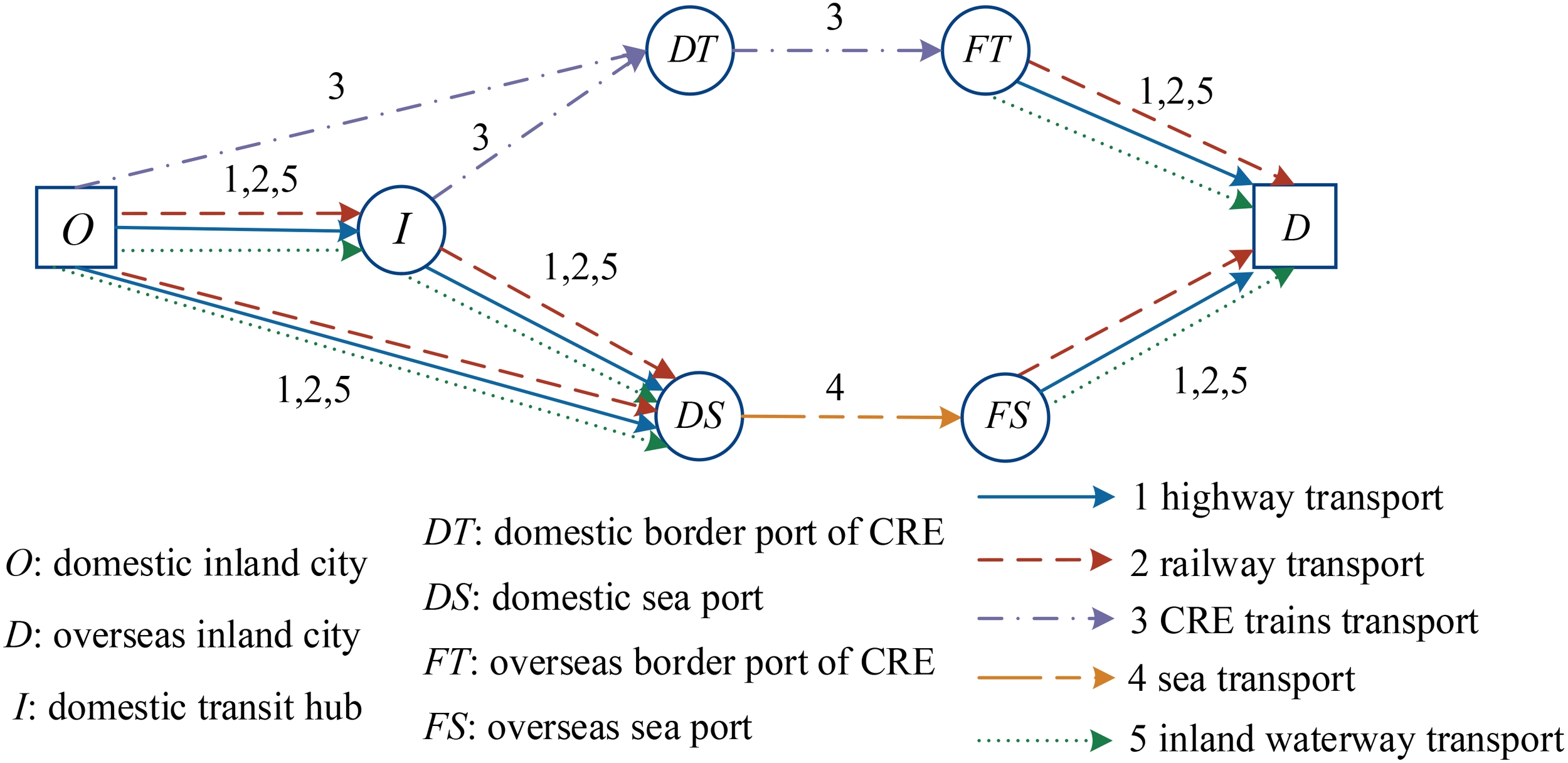
Simplified illustration of the Eurasian container multimodal transportation network.
Thus, the problem to be solved in this paper is to optimize the multimodal route considering the uncertainty and carbon emission constraint. The objectives of the problem are twofold, i.e., minimizing total operation cost and time. Owing to the strong adaptability of the robust technology (Xin et al., 2025), this paper establishes a robust optimization model for the problem.
3.2 Assumptions
-
(1) All container cargoes are transported from origin to destination in a single batch.
-
(2) Only one mode of transport between two nodes can be selected, and the transshipment between different modes can only happen at the transit hub.
-
(3) Transshipment occurs only once at the transit hub. Capabilities of the facilities at the hub for transshipment operation are enough.
-
(4) All transit hubs have a free storage period for container cargoes; thus, we can ignore the waiting cost for transshipment;
-
(5) There are no time windows for the departure of highway, railway, and inland waterway transportation. Sea liners and CRE trains should stick to the schedule.
3.3 Notations
3.3.1 Sets and parameters
O: origin;
D: destination;
N: Set for all the transit hub, therein represents the departure station for domestic liners/CRE trains, ;
V: set for all the nodes in the transport network, ;
: forward node of node i;
: backward node of node;
A: set of arcs in the network, ;
K: set of transport modes,
. The value from 1 to 5 represents highway, railway, CRE trains, sea, and inland waterway transport, respectively, ;
S: set of all scenarios;
Q: number of containers transported between origin and destination;
qs: probability of each scenario, ;
p: parameter of the regret value;
E: constraint of carbon emission for each container;
: connectivity in the multimodal transportation network, i.e., whether container cargoes can be transported from node i to node j by transport mode m. If so, the value should be 1, else 0;
: unit transport cost of a container from node i to node j by transport mode m under scenario s;
: unit transshipment cost of a container from transport mode m to mode n at node i;
: unit transport time from node i to node j by transport mode m under scenario s;
: unit transshipment operation time of a container from transport mode m to mode n at node i under scenario s;
: carbon emission from node i to node j by transport mode m;
: carbon emission from transport mode m to mode n at node i;
: maximum freight volume from node i to node j by transport mode m;
: time window by transport mode m from node i to node j;
: time window of the next period by transport mode m from node i to node j;
: optimal value of the operating cost;
: optimal value of the operating time.
3.3.2 Decision variables
3.3.3 Derived variables
Ti: time when container arrives at node i;
: waiting time for transshipment at node i from transport mode m to mode n.
3.4 Models
3.4.1 Deterministic model
In recent years, research on multimodal transportation route optimization has been continually advancing. Qi (2024) developed a multi-objective route optimization model for rural cold chain logistics in multi-temperature zones, balancing transportation costs, carbon emissions, refrigeration energy consumption, and service quality, making it suitable for small-scale fresh goods. Yang et al. (2024) addressed differences in cargo time sensitivity by introducing mixed time window constraints and designed a bi-level genetic algorithm to optimize container transportation routes, enhancing the model’s adaptability to heterogeneous cargo demands. Huang et al. (2025) developed a multi-objective model considering both transportation costs and time based on Shanghai Port and its hinterland, optimizing the hinterland port access routes using an improved particle swarm algorithm. Ma et al. (2023b) adopted uncertain programming methods to address cross-border transportation under uncertain demand, incorporating factors such as carbon taxes, customs fees, and inland port location selection, and designed a cross-border multimodal transport network model.
In contrast, this study develops a deterministic model (denoted as P1) that focuses on the coordinated optimization of transportation cost, time, and carbon emissions under known demand conditions, specifically in the context of Eurasian container transport—an area that remains underexplored. Unlike previous studies, which often emphasize uncertainty management or heuristic algorithms, our model adopts a deterministic optimization framework to support sustainable transportation decisions from an operator’s perspective. The objective is to minimize both operating cost and time, ensuring efficient and environmentally conscious transport planning across Eurasian corridors.
Objective function:
Constraint condition:
Therein, (Equations 1, 2) are the objective functions of the model. They are minimizing the operating cost and the operating time. The operating cost is the sum of the transport cost of all arcs and transshipment cost at all transit hubs. The operating time is the sum of the transport time of all arcs, the transshipment time at transit hubs, and the waiting time for the transshipment operation. Equation 3 represents the carbon emission constraint in the network. (Equation 4) represents the time when the container actually arrives at node i. (Equation 5) is set to calculate the waiting time for transshipment. (Equations 6, 7) are set to ensure continuity of the transport operation. Among them, (Equation 6) emphasizes that the container must start from O and arrive at D. (Equation 7) is set to ensure the cargo flow balance of the transit hub. Equation 8 is the relationship between the decision variables and the connectivity of the network. Equation 9 asserts that only one mode of transport can be chosen for each arc of the network. Equation 10 shows that only one transshipment can occur at each transit hub. Equation 11 sets the relationship between the decision variables. Equations 12, 13 are set to ensure that all the decision variables are binary variables.
3.4.2 Robust model based on the P-regret value
The P-regret model is a classical method in the field of robust optimization (Raad et al., 2024). It has been widely used in transportation, logistics, and other fields by constraining relative deviation to balance optimization objectives and robustness. Thus, this paper establishes a robust model with the P-regret value. The model should reveal the stochastic characteristics of the transport cost, transport time, and transshipment operation time. We define this model as P2. Compared with the deterministic model (P1), which completely ignores the uncertainty, the P2 model is more suitable for the characteristics of parameter fluctuations in the actual transport network through scene analysis and relative deviation control.
Equations 14, 15 are to minimize the expected value of the operating cost and operating time under all scenarios. The calculation formulas for operating cost and operating time are shown in (Equations 16, 17).
Constraint condition:
For the equations in P2, (Equations 18, 19) are set to ensure that the difference between the objective value with any scenario and the optimal value is in the predetermined scale. Equation 20 is the calculation formula for the time when the container arrives at node i under scenario s. Equation 21 shows how to calculate the waiting time for transshipment under scenario s. (Equation 22) means that the sum of the probability for all scenarios should be one. Furthermore, the model should include Equation 3, and Equations 6 to 13 in P1. As the meanings are the same, we do not need to explain here. Whereas traditional robust optimization typically focuses on minimizing the worst-case objective value, such as in a min–max problem (Baak et al., 2025), the P-regret model introduces a more flexible robustness criterion. Instead of solely optimizing for the worst-case scenario, this model balances expected performance and robustness by incorporating probability-weighted objective functions [Equations 14. 15)] and relative regret constraints [Equations 18. 19)]. This approach ensures that the solution remains stable under uncertainty while avoiding overly conservative decisions that may arise from strict worst-case optimization.
It is important to emphasize that although the objective function of the P-regret model minimizes the overall performance by weighting and summing the objective values across all scenarios, it ensures, through Equations 18, 19, that the relative deviation from the optimal objective value in each scenario does not exceed (1+p) times. In other words, even in the worst-case scenario, the results remain effectively controlled. In contrast, solely adopting a worst-case optimization approach may lead to overly conservative decisions, ultimately reducing overall efficiency. This mechanism ensures that the model’s performance is controlled within an acceptable range across all scenarios, rather than only optimizing for the average case. Therefore, the P-regret model offers significant advantages in balancing average performance and extreme risk mitigation, which is particularly important for practical applications in multimodal transportation networks.
4 Solution algorithm
4.1 Multi-objective genetic algorithm
Multimodal transport networks involve the combination of multiple transport modes, the selection of multiple transit nodes, and complex constraints (such as time windows, carbon emission constraints, etc.) (Yang et al., 2024; Wang et al., 2025b). This study involves two objectives of operating cost and operating time, which are in conflict with each other. The solution method in this paper is based on the improved NSGA-II algorithm proposed by Deb (Deb et al., 2002) in 2002 according to his own NSGA.
As a classic multi-objective optimization algorithm, NSGA-II can generate a set of Pareto optimal solutions (Wang et al., 2025a). Although NSGA-III performs better when dealing with more targets (Hou et al., 2025), its computational complexity is higher. For the problem studied in this paper, the two targets are mainly considered, so NSGA-II is sufficient to cope with it. There are some newer multi-objective optimization algorithms such as MOEA/D (Lin et al., 2017) and SPEA2 (Strength Pareto Evolutionary Algorithm 2) (Lv and Shen, 2023) that may be more suitable for specific types of problems (such as continuous and discrete optimization). However, the problem in this study has the characteristics of mixed integers (involving node selection and transport mode selection), and NSGA-II shows good adaptability in dealing with such mixed problems and achieves a good balance between computational efficiency and quality (Yilmaz et al., 2025).
NSGA-II can effectively deal with two to three objective optimization problems and has mature algorithm implementation and rich application experience, and its stability and reliability have been widely recognized (Ma et al., 2023a). For the large-scale and complex problems in this study, selecting a well-validated algorithm can ensure the reliability of the results. With this in mind, this paper designs NSGA-II to solve the proposed model (Noruzi et al., 2023).
4.2 Basic procedure of the algorithm
The flowchart of the proposed algorithm is shown in Figure 5. The main procedures of the proposed algorithm are as follows.
Figure 5
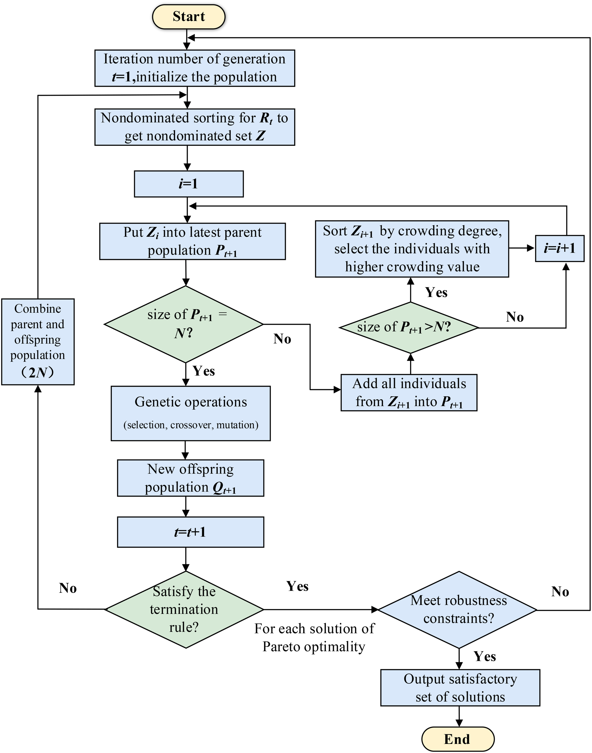
Flowchart of the proposed algorithm.
-
(1) Population initialization. Generate the initial population at random. The scale of the population is set as N. Then, we can get the first generation of the offspring population by the nondominated sorting, selection, crossover, and mutation operation.
-
(2) Population combination. Offspring and their parent are combined to get . The size of the population at this time is . That is twice of the total size N. Because of that, we have to clip the population.
-
(3) Population clipping. Every individual in the new population is nondominated sorted. A series of nondominated set is generated accordingly. The principle of the nondominated sorting is as follows: the lower the layer, the better the individual. Thus, individual is added to until the size of the individual is equal to N. Compare the crowding distance of all individuals in , and choose the individual with the maximum crowding distance.
-
(4) Iterative operation. We conduct operations of selection, crossover, and mutation to the new parent population. In this way, we can get new offspring population. Repeat the step below until the termination rule is satisfied. Then, we can get the Pareto solution set.
-
(5) Validation of the robustness. Based on the robustness of the proposed model, this paper applies the validation of the robustness apart from the normal procedure of NSGA-II. If there is solution satisfying the robustness constraint in the Pareto set, then we decode the solution and get the optimal robust scheme. Otherwise, we return to the beginning of the algorithm and repeat the procedure.
4.3 Key operators of the algorithm
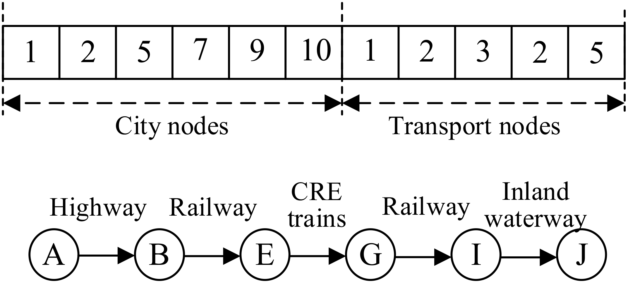
(1) Chromosome coding
There are five modes of transport in the multimodal network. Based on that characteristic, this paper determines the chromosome encoding method as a chain composed of two parts: transport city nodes and transportation modes. The first part is made up of the node cities. Thus, the length of the first part is the number of the node cities in the scheme. The second part is set to represent the transport mode between the node cities. Thus, the length of the second part is equal to the length of the first part minus 1. We can see the illustration from the upper half of Figure 6. Suppose there are 10 nodes in the network (1–10 representing city A–J), and there are 5 types of transportation modes available between all nodes: highway, railway, CRE trains, sea, and inland waterway. Real numbers are used to encode the node cities, represented by 1, 2, 3, 4, 5, 6, 7, 8, 9, and 10 for the 10 city nodes; similarly, real numbers are used to encode the transportation modes, represented by 1, 2, 3, 4, 5 for highway, railway, CRE trains, sea, inland waterway. For example, the encoding format “1-2-5-7-9-10-1-2-3-2-5” indicates that the transportation sequence of cities is A-B-E-G-I-J. Goods are transported from city node A to node B by road, then to node E by rail, and between node E and node G by sea, between node G and node I by rail, and between node I and node J by inland waterway. There are transportation mode conversions at nodes B, E, G, and I, as shown in the lower part of Figure 6.
Figure 6
Schematic diagram of chromosome coding.
(2) Generation of the initial population
The initial population is generated at random. However, during the initialization process, it is necessary to check if the population meets the feasibility constraints. For example, if there is connectivity between two nodes, then we should eliminate the individual. Moreover, to ensure the size of the population maintain at N, we should supplement the corresponding number of illegible individuals.
(3) Nondominated sorting
The operation of nondominated sorting is the classification of population hierarchy according to different relationships between domination and nondomination. In multi-objective programming, if at least one of the objectives of individual p is better than that of individual q, and other objectives of individual p is no worse than those of individual q, then we can say that the individual p dominates individual q. Individual q is called nondominated solution or Pareto solution. All the nondominated solutions are classified as the first layer, labeled with the value of grank = 1. Then, the second layer of the nondominated solutions is sorted out from the remaining individuals, labeled with grank = 2. Likewise, the nondominated sorting is conducted until all the individuals are labeled.
(4) Calculation of the crowding distance
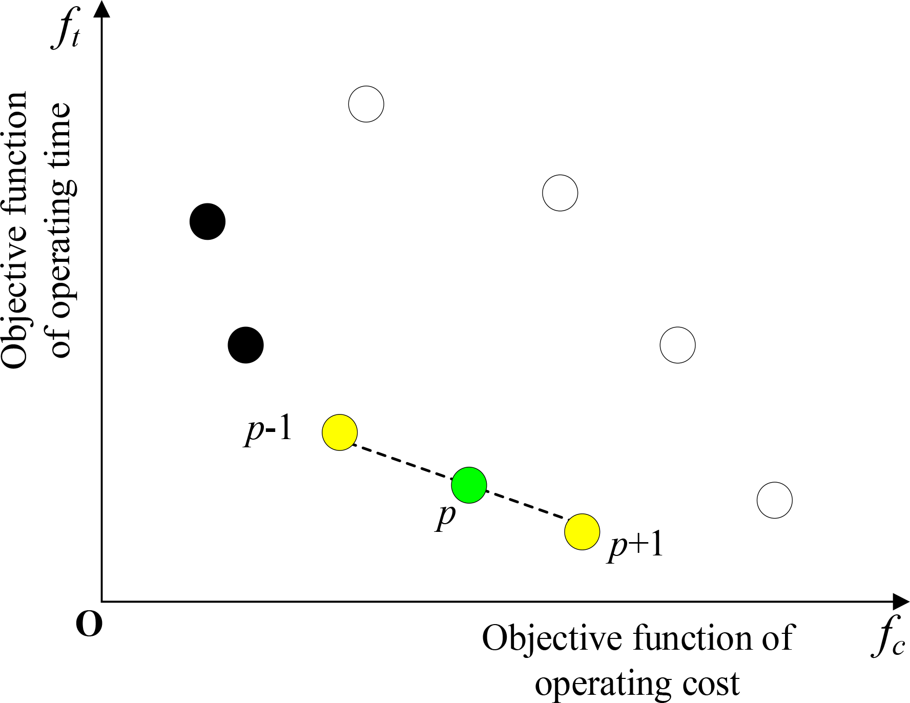
The lower the nondominated layer, the better individuals in that layer are. If we want to know which of the individuals in the same layer is better, we may consider an internal sorting by crowding distance. The crowding distance of individual p means the three-dimensional Euclidean distance of two neighborhood individuals of p, i.e., p+1 and p−1. The calculation method is shown in (Equation 23).
Therein, and are two objective function values of the model about operating cost and operating time, respectively. means the value of the objective function – operating cost for individual p+1. Figure 7 can be the illustration of crowding distance for individual p. We can take the length of the dotted line from p−1 to p+1 as the crowding distance for p. Obviously, the bigger the value of , the more diversified the population is.
Figure 7
Crowding distance of individual p.
(5) The selection operation
This paper adopts the tournament method for the selection operation. The method is based on the value of the layer and crowding distance. By comparing individuals’ non-dominant rank and crowding distance, tournament selection is able to preferentially select high-quality individuals while maintaining population diversity. More specifically, we compare values of the layer (the value of grank) between the two individuals first. If the values are different, then we choose the individual with a lower value of the layer. At this point, we do not need to consider the crowding distance. Otherwise, if the values of the layer are the same for the two individuals, then we should calculate the crowding distance. The individual with the bigger crowding distance should be selected, so that the diversification of the population can be maintained. This method is widely used in many multi-objective optimization algorithms and proved to be effective. For example, Deb et al. (2002) described in detail the advantages of tournament selection in the original paper of the NSGA-II algorithm, especially the ability to effectively balance convergence and diversity when dealing with multi-objective optimization problems. In addition, Kim et al. (2004) also verified the stability and effectiveness of tournament selection in problems of different sizes and complexities through experiments.
(6) The crossover operation
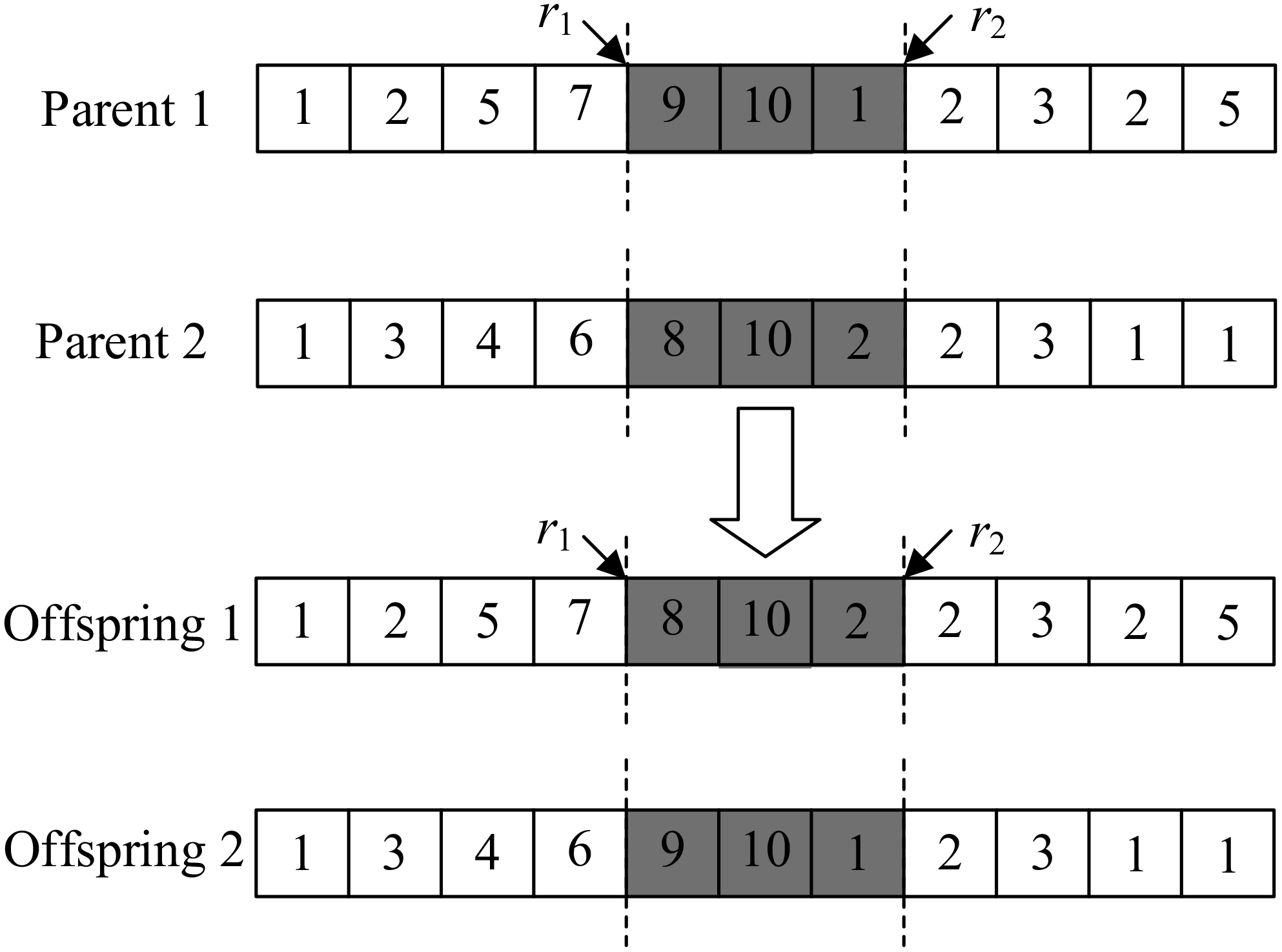
The two-point operator is adopted in this paper for the crossover operation. This choice is based on its wide application and good performance in combinatorial optimization problems. By exchanging gene segments between two random locations in two parent chromosomes, the two-node crossover operator can effectively explore the new solution space while maintaining the structural stability of the solution. The detailed process is as follows. Two integers ranging from 2 to n−1 (n is the length of the chromosome) are generated at random. These two integers are named r1 and r2 in ascending order. Extract the gene segments between r1 and r2 extracted from the two parents and interchange them. The other segments remained unchanged. Thus, we can get two new chromosomes. The crossover operation is shown in Figure 8. This approach has been shown to be effective in many studies, especially when dealing with path- or sequence-dependent optimization problems. For example, Campuzano et al. (2025) and Singgih and Singgih (2024) pointed out in their research that two-node crossover operators can maintain the consistency of solutions and produce high-quality offspring solutions when solving path optimization problems such as traveling salesman problem (TSP) and vehicle routing problem (VRP). Notably, Lim et al. (2021) further validated the advantages of two-point crossover in complex logistics network optimization through their recent study on the multi-depot split-delivery vehicle routing problem (MDSDVRP). By constructing a two-dimensional chromosome encoding and dynamic mutation strategies, combined with Taguchi parameter optimization methods, this research demonstrated that two-point crossover can effectively maintain solution consistency and enhance global search capabilities under scenarios requiring multi-depot collaborative scheduling and multiple-delivery constraints.
Figure 8
Schematic diagram of the chromosome crossover operation.
(7) The mutation operation
The mutation operation can be described as follows. Firstly, a random number in the scope of [0,1] is generated. Then, the number is compared with the mutation probability. If the number is lower than the mutation probability, then a single-point mutation operation is adopted. Randomly generate a gene point r and change the value at the point to another value in the candidate number set. If not, the parent will remain unchanged. The single-point mutation operation is shown in Figure 9. Single-point variation can be explored on a local scale by randomly changing a gene location in the chromosome and increasing the diversity of solutions while avoiding excessive structural changes that lead to the loss of solution viability. This method is very common in the application of genetic algorithms and has been validated in many studies. For example, Yi et al. (2018) pointed out in their study that when dealing with combinatorial optimization problems, single-point mutation operators can effectively jump out of local optimality without destroying the basic structure of the solution. In addition, they also showed through experiments that single-point variation can help the algorithm better maintain the diversity of the population in multi-objective optimization problems, thus improving the global search ability. To ensure the feasibility of the chromosome after mutation, all the values in the candidate set should satisfy the connectivity requirements between related cities considering the transport mode.
Figure 9
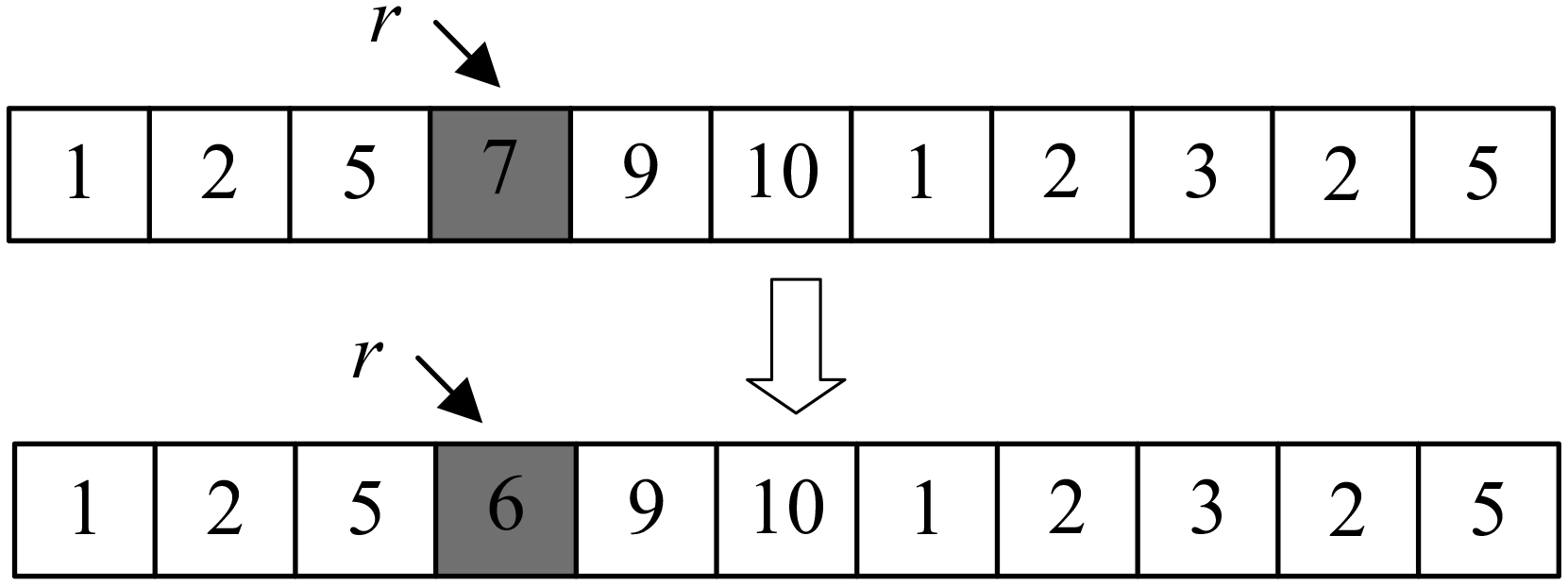
Schematic diagram of mutation operation.
(8) Population combination and clipping
The combination of parents and offspring can guarantee that good solutions can inherit afterwards. However, the size of the population becomes twice of the original size after the combination. Thus, it is necessary to conduct the clipping operation so that the size of the population remains unchanged. The procedure for the clipping operation is as follows.
-
Step 1: initialize the number of permitted individuals (PS) as N.
-
Step 2: check the size of current nondominated set with the minimum value of grank (NM).
-
Step 2.1: If NM is no bigger than PS, then all the dominated solutions are included into the new population. The value of PS will be updated as PS minus NM. Explore the nondominated layer with the higher ordinal value (grank+1) and end the clipping procedure until the value of PS reaches zero.
-
Step 2.2: If NM is bigger than PS, then sort all the individuals of the current layer according to the crowding distance in descending order and choose the first PS individuals into the new population. End the clipping procedure.
5 Empirical analysis
5.1 Data
5.1.1 Network description
Nanjing is the national comprehensive transportation hub of China. It has an intensive highway network and a developed waterway network. Furthermore, the two-way trade between China and Germany has reached 205.7 billion Euro. China has become the most important trading partner for 4 years. Thus, this paper takes the transportation of 40 FEU containers from Nanjing, China (denoted as O) to Berlin, Germany (denoted as D) as the example in empirical study. Three corridors for chosen have been introduced in Figures 1–3 in Section 1. The multimodal network from Nanjing to Berlin in detail is shown in Figure 10.
Figure 10
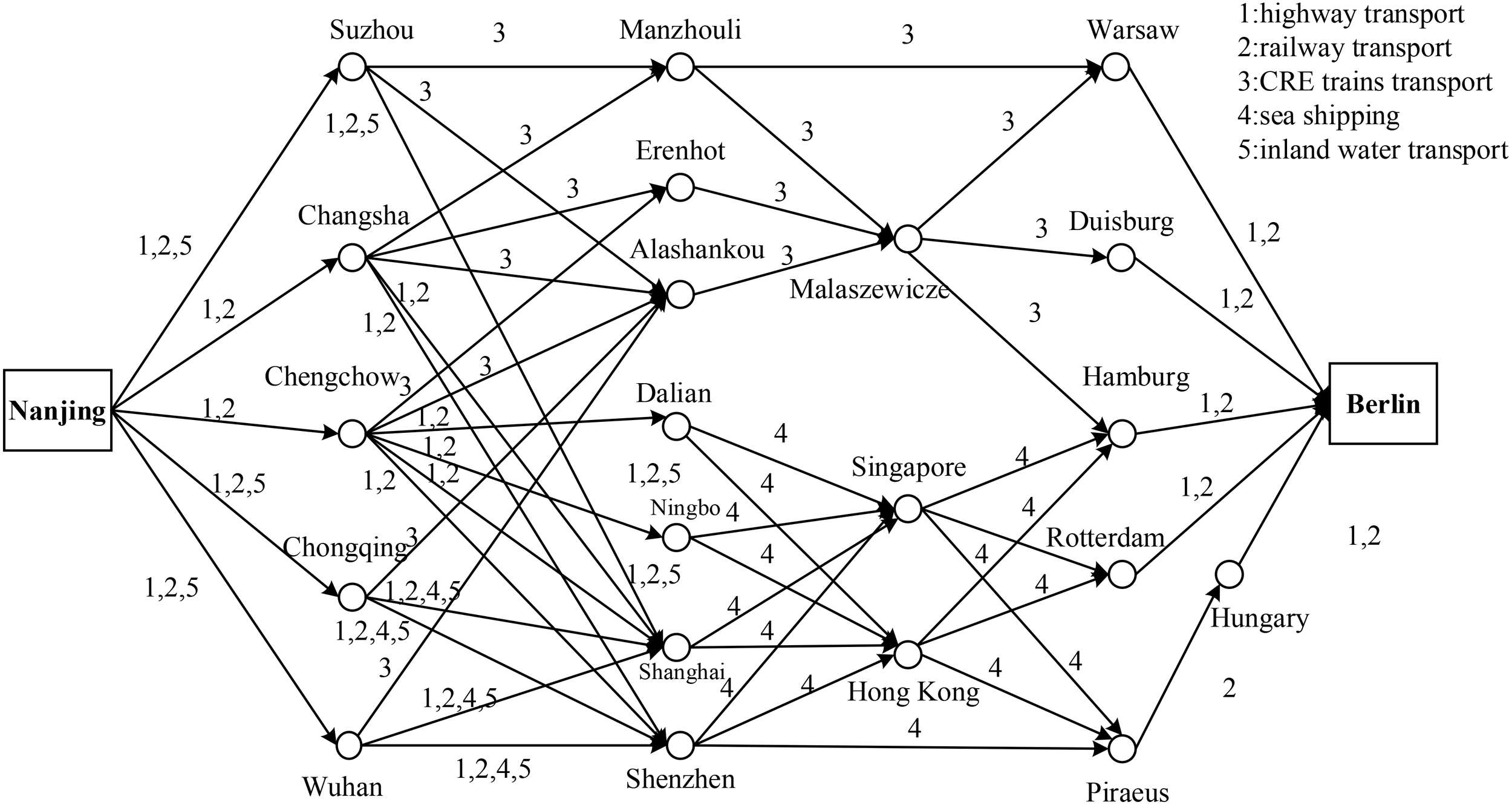
Container multimodal transportation network from Nanjing to Berlin.
As shown in Figure 10, according to the routes of the CRE trains, Manzhouli, Erenhot, and Alashankou are selected as three border ports (DT). According to the ranking of the Chinese container ports and main ports concerning China–EU container transportation, Dalian, Shanghai, Ningbo, and Shenzhen are selected as domestic sea ports (DS). Based on the destinations of the three main corridors of CRE trains and sea ports, Warsaw, Duisburg, Hamburg, Rotterdam, and Piraeus are selected as foreign border ports (FT) and sea ports (FS). Suzhou, Changsha, Chengchow, Chongqing, and Wuhan are selected as candidate transit hubs (I). Considering that Hong Kong and Singapore rank as the top two in terms of current container transshipment volume, this paper chooses the two ports as ports of call. Moreover, as any CRE routes will have to change rail at Malaszewicze, we select this city as the overseas border port. For simplified description of the transport scheme in the following part, we allocate code numbers for all the city nodes, as shown in Figure 10.
5.1.2 Data description
For the calculation of carbon emission, we assume that an FEU container is equal to 30 tons of container cargoes. Furthermore, as many multimodal operations are settled by US dollars, we set the exchange rate between US dollar and RMB as 7 for unity. Related data for the study are as follows. The city codes of the China-Europe Container Transport Corridor are shown in Table 1 below.
Table 1
| Code | City | Code | City | Code | City | Code | City |
|---|---|---|---|---|---|---|---|
| 1 | Nanjing | 7 | Dalian | 13 | Alashankou | 19 | Hamburg |
| 2 | Suzhou | 8 | Shanghai | 14 | Singapore | 20 | Rotterdam |
| 3 | Changsha | 9 | Ningbo | 15 | Hong Kong | 21 | Piraeus |
| 4 | Chengchou | 10 | Shenzhen | 16 | Malaszewicze | 22 | Hungary |
| 5 | Chongqing | 11 | Manzhouli | 17 | Warsaw | 23 | Berlin |
| 6 | Wuhan | 12 | Erenhot | 18 | Duisburg |
The code of cities in the China–EU container transportation corridor.
(1) Freight rates
Freight rates are different according to different modes of transport and zones. For road transport in the Chinese region, the basic freight rate of a 40-ft container is 9 yuan/FEU• km, and additional charge for a container is 25 yuan/FEU. Freight rate in the overseas region is $2/FEU• km. Container rates of sea and inland waterway transport are $0.25/FEU• km and $0.15/FEU• km. For railway transport, freight rates are listed in Table 2.
Table 2
| Zone | Freight rate (FEU container) |
|---|---|
| Chinese zone | Basic freight of delivery is 680 yuan/FEU, and basic freight of operation is 2.754 yuan/FEU• km |
| CIS zone | Freight rates departing from Manzhouli, Erenhot, and Alashankou are $0.41/FEU• km, $0.44/FEU• km and $0.69/FEU• km |
| EU zone | Unified freight rate in EU zone is $1/FEU• km |
Freight rates for railway transport of different zones.
Source: China Economic Information Service.
(2) Transport time
Transport time is equal to the ratio of transport distance to speed. As to the highway and railway distance, we get the data from Google Earth. The waterway route distances are achieved by Netpas Distance. We set 100 km/h as the maximum speed of highway transport, and the relationship factor of average to maximum speed is 0.75. The maximum speed of containership is set as 25 knots, i.e., 46 km/h, and the relationship factors of sea and inland waterway transport are 0.8 and 0.6, respectively. The maximum speed of railways is 100 km/h. The average speed of different zones is different, as shown in Table 3.
Table 3
| Railway transport zone | Relationship factor of average to maximum speed | Average speed (km/h) |
|---|---|---|
| Chinese zone | 0.70 | 70 |
| CIS zone | 0.52 | 52 |
| EU zone | 0.60 | 60 |
Average speed of railway transport in different zones.
(3) Carbon emission during the transport process
Carbon emission parameters are classified only in three ways, i.e., road, rail, and water. Thus, railway and CRE trains are treated the same, and sea and inland waterway transport are taken identically. Related parameters are shown in Table 4.
Table 4
| Mode of transport | Consumption of standard coal (Em) kg/t• km | Emission factor of CO2 (P) kg CO2/GJ | Calorific value of standard coal (CE) kg/GJ | Carbon oxidation factor (α) |
|---|---|---|---|---|
| Highway | 20 × 10−6 | 94.6 | 29.3076 | 1 |
| Railway/CRE trains | 4.11 × 10⁻⁶ | |||
| Sea/Inland waterway | 2.2 × 10⁻⁶ |
Carbon emission parameters for different modes of transport.
Source: Statistical bulletin on the development of China’s transportation industry.
(5) Transshipment operation-related data
Related data about the transshipment operation is calculated using the real life transshipment cost, time, and carbon emission. They are shown in Table 5.
Table 5
| Highway | Railway | CRE trains | Sea | Inland waterway | |
|---|---|---|---|---|---|
| Highway | —— | 5/0.3/0.5 | 5/0.3/0.5 | 5/0.3/0.8 | 5/0.3/0.8 |
| Railway | 5/0.3/0.4 | —— | 7/0.5/0.6 | 10/0.8/1 | 10/0.8/1 |
| CRE trains | 5/0.3/0.4 | 7/0.5/0.6 | —— | 10/0.8/1 | 10/0.8/1 |
| Sea | 5/0.3/0.7 | 10/0.8/1 | 10/0.8/1 | —— | 8/0.7/0.8 |
| Inland waterway | 5/0.3/0.7 | 10/0.8/1 | 10/0.8/1 | 8/0.7/0.8 | —— |
The transshipment cost, time, and carbon emissions between transportation modes.
Data format is “a/b/c”. a: transshipment cost (yuan/t); b: transshipment time (h/FEU); c: Emission factor (kg/t). “—” means that transshipment cost/time/emission can be ignored between the same mode of transport.
(6) Time windows of liners and CRE trains
We define the beginning of the planning time as zero, and the unit of time is an hour. Table 6 is the departure time window of liners and CRE trains.
Table 6
| City nodes of the CRE departure station | Transportation schedule | City nodes of departure port for liners | Transportation schedule | ||
|---|---|---|---|---|---|
| 1 | 2 | 1 | 2 | ||
| 2 | [0,48] | [48,96] | 7 | [36,84] | [84,132] |
| 3 | [12,60] | [60,108] | 8 | [36,84] | [84,132] |
| 4 | [12,60] | [60,108] | 9 | [48,96] | [96,144] |
| 5 | [24,72] | [72,120] | 10 | [48,96] | [96,144] |
| 6 | [24,72] | [72,120] | |||
Time windows of liner ships and CRE trains.
Take the time window of [12, 60] of node 3 as the example. It means that the CRE train arrives at 12 and leaves at 60. If container cargoes arrive before 12, we will have to wait until 12 to operate the transshipment operation. If container cargoes arrive between 12 and 60, and finish the transshipment operation, then the container cargoes can leave at 60. However, if container cargoes arrive after 60, or has not completed the transshipment operations, it can only choose the second transportation schedule, the train with a time window of [60, 108].
(7) Generation of the stochastic disturbance data
Based on the parameters introduced previously, we can get the transport time, cost, and operation time for transshipment at all transit hubs. The data are set as the basic data. Four disturbance data are generated by a different disturbance level based on the basic data. The levels are ±10%, ± 20%, ± 30%, and ±40%, respectively. Combined with the basic scenario, we get five scenarios. Assume that the probabilities for the five scenarios are 0.4, 0.2, 0.2, 0.1, and 0.1 respectively. The regret value is set as 0.5.
5.2 Results analysis
5.2.1 Model and algorithm validation
We use the CPLEX to validate the model. The operating system is Windows 10 with an Intel Core I5-8300H CPU@2.30GHz processor. A small-scale case is used to validate the feasibility of the proposed model and related variables. Basic information of the small-scale case is as follows. Fifteen city nodes (1, 2, 4, 5, 7, 8, 10, 11, 13, 18, 19, 20, 21, 22, and 23), one basic scenario, and three modes of transport (1: highway; 2: railway; 4: sea) are considered. As CPLEX can only solve the single-objective model, we transform the bi-objective to single-objective model by setting weights of the two objectives as 0.5. Constraint of CO2 emission for each container is set as 2500 kg. Table 7 is the optimal multimodal scheme. The transport route and mode conform to reality, which proves the feasibility of the proposed model in this paper.
Table 7
| Transport route | Transport mode | Operating cost/$ | Operating time/h |
|---|---|---|---|
| 1-2-8-21-22-23 | 2-2-4-2-2 | 79295.8 | 559.3 |
Optimal transportation scheme and relevant data of multimodal transportation.
We use the NSGA-II to solve the same case. Parameters for the algorithm are set as follows. Population size is 100, maximum number of iterations is 500, and the probabilities for crossover and mutation are 0.8 and 0.1, respectively. After executing the algorithm, we obtain a set of Pareto optimal solutions. Table 8 presents a subset of these solutions.
Table 8
| Scheme | Transport route | Transport mode | Operating cost/$ | Operating time/h |
|---|---|---|---|---|
| 1 | 1-2-8-19-23 | 2-4-4-1 | 72,739.5 | 708.1 |
| 2 | 1-2-9-19-23 | 2-4-4-1 | 72,243.0 | 712.4 |
| 3 | 1-4-7-19-23 | 2-2-4-1 | 73,326.6 | 703.9 |
| 4 | 1-2-8-21-22-23 | 2-2-4-2-2 | 79,295.8 | 559.3 |
| 5 | 1-2-10-21-22-23 | 2-2-4-2-2 | 79,778.6 | 554.7 |
| 6 | 1-2-8-21-22-23 | 1-4-4-2-2 | 81,562.1 | 542.0 |
| 7 | 1-4-7-21-22-23 | 2-2-4-2-2 | 80,914.3 | 549.4 |
Pareto optimal solution set.
A decision-maker can select the optimal scheme based on specific requirements. For cost-sensitive scenarios, the first three options are preferable. These primarily utilize sea transport, supplemented by highway and railway connections. Compared to scheme 6, these options can reduce operating costs by up to 12.5%. Conversely, if minimizing process duration is the priority, the last four schemes are the most suitable. These routes largely leverage the China–EU sea–land express corridor, reducing operating time by up to 25%.
Furthermore, we get the normalized scheme from the seven schemes in Table 8, as shown in Table 9. Analyzing the normalized f(x), we get the minimum value from scheme 4. The result is the same with that from CPLEX. Thus, we can see that the transport scheme mainly concerning the China–EU sea–land express corridor is better considering economics and timeliness.
Table 9
| Scheme | Transport route | Transport mode | |||
|---|---|---|---|---|---|
| 1 | 1-2-8-19-23 | 2-4-4-1 | 0.05 | 0.97 | 0.51 |
| 2 | 1-2-9-19-23 | 2-4-4-1 | 0.00 | 1.00 | 0.50 |
| 3 | 1-4-7-19-23 | 2-2-4-1 | 0.12 | 0.95 | 0.53 |
| 4 | 1-2-8-21-22-23 | 2-2-4-2-2 | 0.76 | 0.10 | 0.43 |
| 5 | 1-2-10-21-22-23 | 2-2-4-2-2 | 0.81 | 0.07 | 0.46 |
| 6 | 1-2-8-21-22-23 | 1-4-4-2-2 | 1.00 | 0.00 | 0.50 |
| 7 | 1-4-7-21-22-23 | 2-2-4-2-2 | 0.93 | 0.04 | 0.49 |
Normalized value of Pareto optimal solution.
To testify the effectiveness of the proposed algorithm, this paper conducts four case analyses considering different scales. The scales of the four cases are shown in Table 10. They are solved by both CPLEX and NSGA-II. The results are shown in Table 11 and Figure 11. For large-scale problems, NSGA-II takes significantly less time to compute than CPLEX (as shown in Figure 11) and is able to generate a set of high-quality Pareto optimal solutions. This demonstrates the efficiency and effectiveness of NSGA-II in dealing with large-scale, complex problems.
Table 10
| Case number | Case scale | ||
|---|---|---|---|
| Number of nodes | Number of scenarios | Number of transport modes | |
| 1 | 15 | 1 | 3 |
| 2 | 23 | 1 | 3 |
| 3 | 23 | 1 | 5 |
| 4 | 23 | 5 | 5 |
Scale of the four cases.
Table 11
| Case number | Objective value of operating cost Objective value of operating time | ||||||
|---|---|---|---|---|---|---|---|
| CPLEX | NSGA-II | Gap* | CPLEX | NSGA-II | Gap* | ||
| 1 | 79,295.8 | 79,295.8 | 0 | 559.3 | 559.3 | 0 | |
| 2 | 80,421.3 | 80,421.3 | 0 | 565.3 | 565.3 | 0 | |
| 3 | 81,262.9 | 81,624.4 | 361.5 | 572.5 | 583.6 | 11.1 | |
| 4 | 81,319.7 | 81,940.2 | 620.5 | 540.2 | 567.6 | 27.4 | |
Comparison of results solved by CPLEX and NSGA-II for different cases.
Gap*: is the result from NSGA-II minus the result from CPLEX.
Figure 11
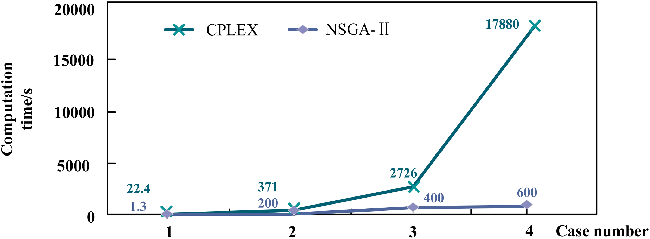
Comparison of CPLEX and NSGA-II computation time for different cases.
We can see from Table 11 that when the case scale is relatively small, the objective values obtained from CPLEX and NSGA-II are very close, or even the same. That reveals the fact that the NSGA-II algorithm can achieve high precision when dealing with small-scale problems. According to Zeinab Aliahmadi et al. (2025) and Ma et al. (2023c), the verification of multi-objective algorithms should focus on the combined complexity gradient of decision variables, constraints, and objective functions, rather than simply pursuing the number of instances. Through systematic changes in the number of nodes (15–23), the number of scenarios (1–5), and the number of transportation modes (3–5), these four cases have basically covered the typical complexity range of logistics network optimization (Zhu et al., 2024). This result is consistent with previous studies (Pak et al., 2022), which also found that NSGA-II showed high accuracy in dealing with small-scale optimization problems. This validates the applicability of NSGA-II in multimodal transport networks, especially in small-scale scenarios.
Moreover, although the computation time of CPLEX is acceptable when the case scale is small, when the scale increases, the complexity of the problem increases a lot. That fact leads to the phenomenon of sharp increase of computation time by CPLEX. From case 1 to case 4, introducing eight additional nodes, four scenarios, and two transportation modes led to an exponential increase in CPLEX’s computational solution time, exhibiting a “jump” phenomenon. As illustrated in Figure 11, the solution time for case 4 already required nearly 5 h. In contrast, the computational time growth of NSGA-II remained relatively gradual. That leads to the conclusion that NSGA-II has a great advantage on solving large-scale problems.
5.2.2 Comparison between the single-objective and multi-objective model
Figures 12 , 13 show the comparison between single-objective and multi-objective models under different scenarios. If we take the operating cost as the analysis object, we can see that the optimal cost under the single objective of operating cost is only about 70 million dollars. However, that value is up to nearly 130 million dollars, while the operating cost is about 80 million dollars. That value only exceeds 15% of the optimal value of the single objective, which is quite satisfactory. The situation about the operating time is similar. Under single-objective circumstances, the average optimal values of the five scenarios are 436 and 763 h, while that value is about 566 h in our multi-objective model, which exceeds 29% of the optimal value of the single-objective model. That is also satisfactory to some degree.
Figure 12
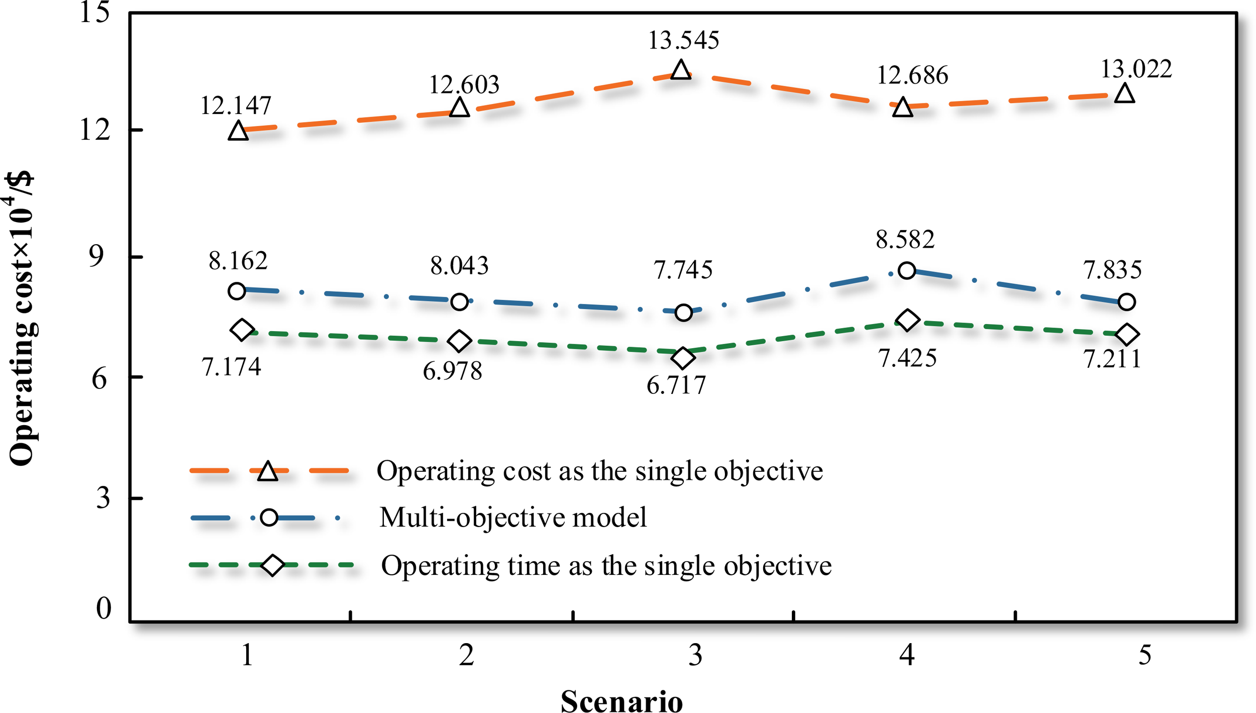
Comparison of the total cost between the single-objective and multi-objective model.
Figure 13
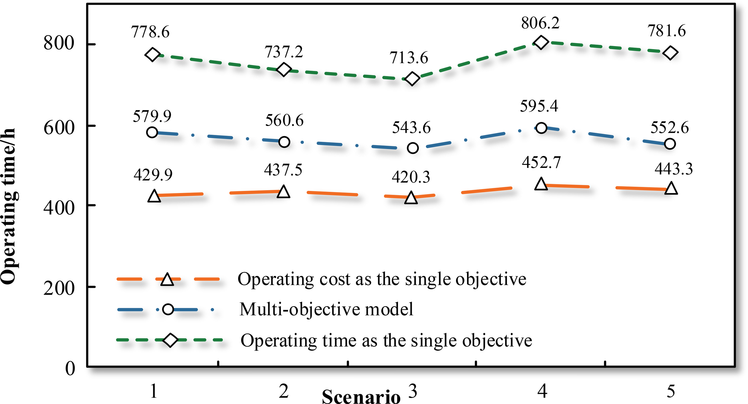
Comparison of the total time between the single-objective and multi-objective model.
Thus, it is evident that the two objectives are inherently conflicting, potentially even mutually exclusive. Consequently, achieving optimal values for both objectives simultaneously using a single-objective model is not feasible. Improving one objective inevitably leads to a degradation in the other. Multi-objective optimization offers a framework for achieving a compromise and trade-off between these competing objectives, allowing each objective to approach its optimal value as closely as possible.
5.2.3 Comparison between the robust and deterministic model
To solve the P-regret value robust model, we have to obtain the optimal values of the two objectives under different scenarios. The minimum values of operating cost and time under all scenarios are and in Tables 12, 13. Likewise, the maximum values of operating cost and time under all scenarios are and . In Tables 12, 13, values of and are the objective functions in P2 under scenario s. Relative deviations of operating cost and time are calculated as follows.
Table 12
| Scenario | Fluctuation level | Value of operating cost | Relative deviation | ||
|---|---|---|---|---|---|
| 1 | No fluctuation | 71,739.5 | 143,868.2 | 82,814.9 | 15.4% |
| 2 | [0.9–1.1] | 69,784.2 | 148,959.4 | 80,431.1 | 15.3% |
| 3 | [0.8–1.2] | 68,970.1 | 159,216.1 | 77,890.9 | 12.9% |
| 4 | [0.7–1.3] | 74,251.9 | 145,848.9 | 86,275.9 | 16.2% |
| 5 | [0.6–1.4] | 72,105.7 | 158,202.7 | 79,017.5 | 9.6% |
Relative deviation of the operating cost of the robust optimization model and the determinate model under various scenarios.
The relative deviation is calculated using (Equation 24).
Table 13
| Scenario | Fluctuation level | Value of operating time | Relative deviation | ||
|---|---|---|---|---|---|
| 1 | No fluctuation | 429.9 | 822.4 | 538.1 | 25.0% |
| 2 | [0.9–1.1] | 437.5 | 810.3 | 545.6 | 24.7% |
| 3 | [0.8–1.2] | 420.3 | 879.6 | 522.5 | 24.3% |
| 4 | [0.7–1.3] | 452.7 | 929.9 | 565.1 | 24.8% |
| 5 | [0.6–1.4] | 443.3 | 896.9 | 548.0 | 23.6% |
Relative deviation of the operating time of the robust optimization model and the determinate model under various scenarios.
The relative deviation is calculated using (Equation 25).
For example, calculate the relative deviation of operating cost in S2. According to Table 12, the minimum operating cost for Scenario 2 is 69,784.2, and the objective function value is 80,431.1. Using (Equation 24) to calculate the relative deviation results in a value of 15.3%.
The relative deviations in Tables 12 and 13 demonstrate that the P2 model effectively limits performance degradation across all scenarios. For example, even under the widest fluctuation (Scenario 5, ± 40%), the operating cost and time remain within 25% of the deterministic solution, validating the model’s resilience against uncertainty.
5.2.4 Analysis of different fluctuation situations
The five scenarios previously analyzed are generated at random based on the basic data. The fluctuation levels are 0, ± 10%, ± 20%, ± 30%, and ±40%, respectively. The probabilities for each scenario are 0.4, 0.2, 0.2, 0.1, and 0.1 respectively. The situation is defined as S1. In this section, we set another fluctuation situation and compare it with the original optimal scheme. This situation is called S2. Descriptions of S2 are as follows. Five scenarios are generated based on the basic data, with all fluctuation levels of ±40%. Probabilities for each scenario are all 0.2. Table 14 shows the optimal scheme under two fluctuation situations.
Table 14
| Situation | Transport route | Transport mode | Operating cost/$ | Operating time/h |
|---|---|---|---|---|
| S1 | 1-2-8-15-21-22-23 | 2-1-4-4-2-1 | 81,319.7 | 540.2 |
| S2 | 1-2-8-15-21-22-23 | 2-1-4-4-2-1 | 80,431.0 | 551.7 |
Comparison results under different fluctuation situations.
It can be seen from the comparison that, even if the fluctuation situation changes, the optimal transport scheme remains unchanged. The proposed transportation scheme maintains its core structure: railway transport from Nanjing to Suzhou, followed by highway transport to the Port of Shanghai, and sea transport via Singapore to the Port of Piraeus through the China–EU sea–land express corridor, with subsequent railway transport to Hungary and highway transport to Berlin. While the optimal total operating cost and time differ from the deterministic case, the values remain within acceptable bounds. This resilience demonstrates the P-robust model’s capability to mitigate the effects of uncertain factors and maintain operational stability.
5.2.5 Sensitivity analysis of the related parameters
To testify the influence of the parameters on the model, this section sets three cases with different situations of carbon emission constraints, time windows, and regret values of p.
(1) Sensitivity analysis of carbon emission constraints
This section compares the results of four different carbon emission constraints. The four constraints are strict constraint (E = 2,500), relatively strict constraint (E = 3,000), moderate constraint (E = 3,500), and loose constraint (E = 4,000). Firstly, we get 29 Pareto solutions by relaxing the emission constraint. The solutions form the Pareto frontier curve. The curve is the compromise between operating cost and time. Then, we add the carbon emission constraint. In this way, we can observe the change of the solution space, as shown in the bolded points from Figures 14–17.
Figure 14
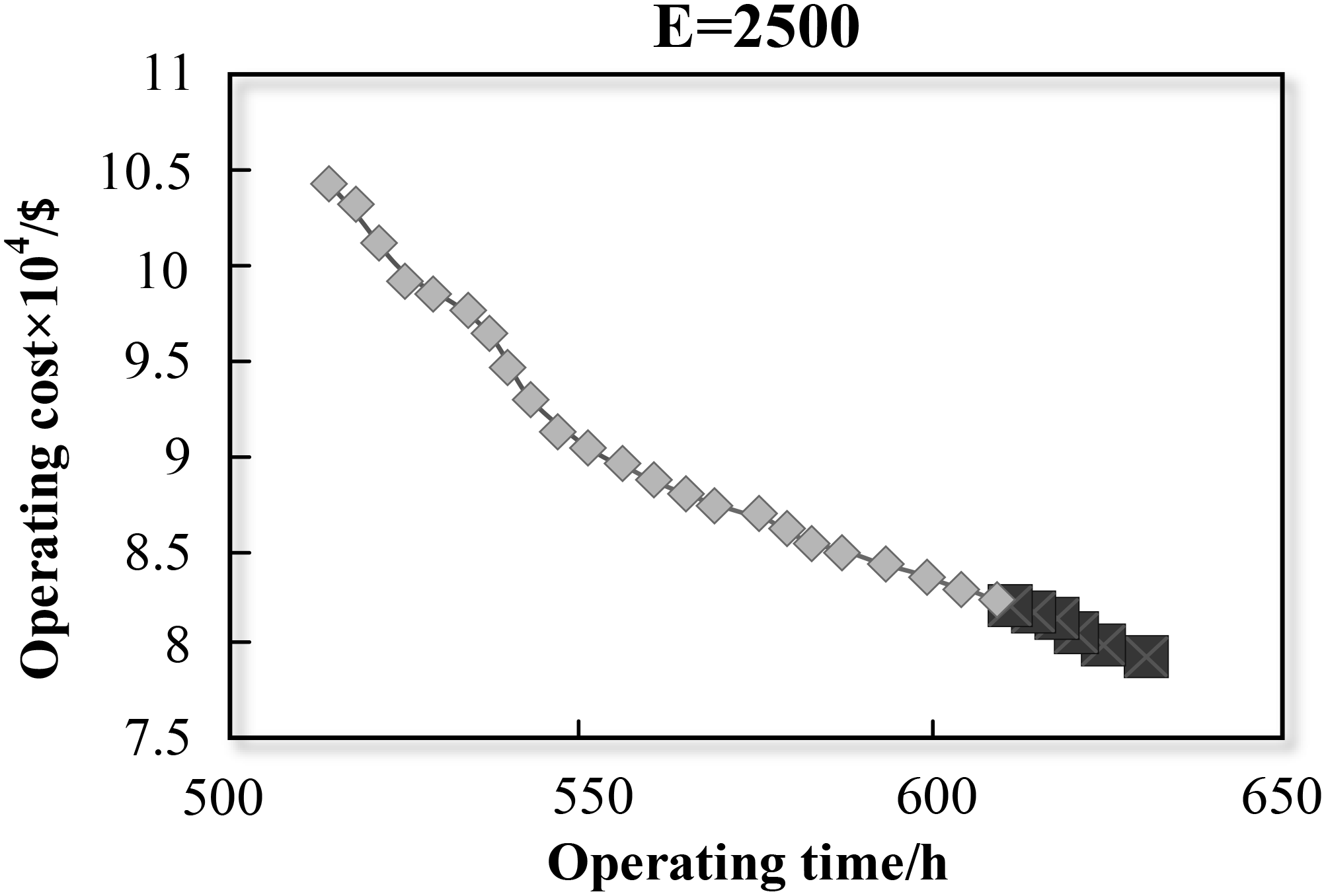
Modeling results at carbon emissions constraint I (E = 2,500).
Figure 15
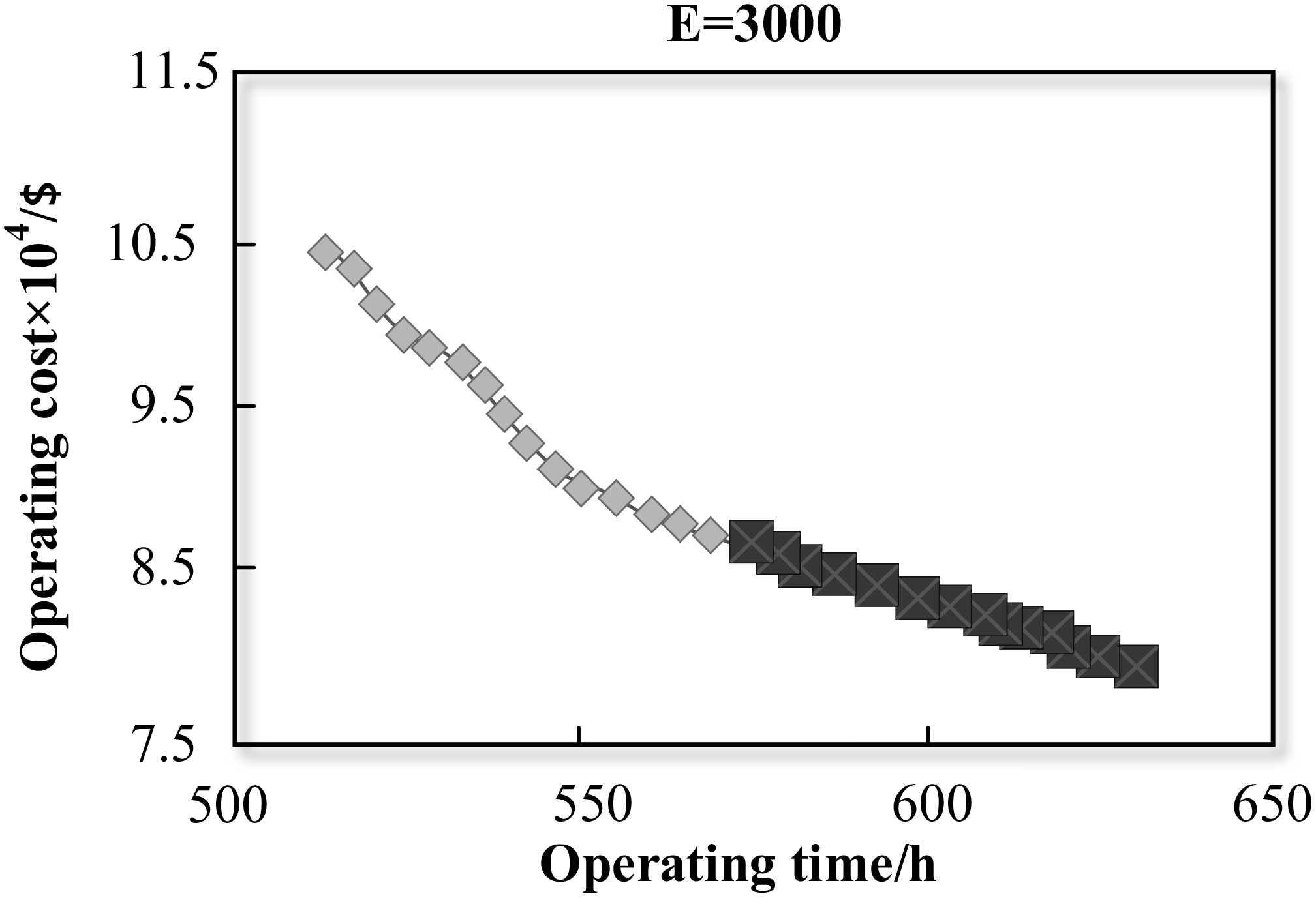
Modeling results at carbon emissions constraint II (E = 3,000).
Figure 16
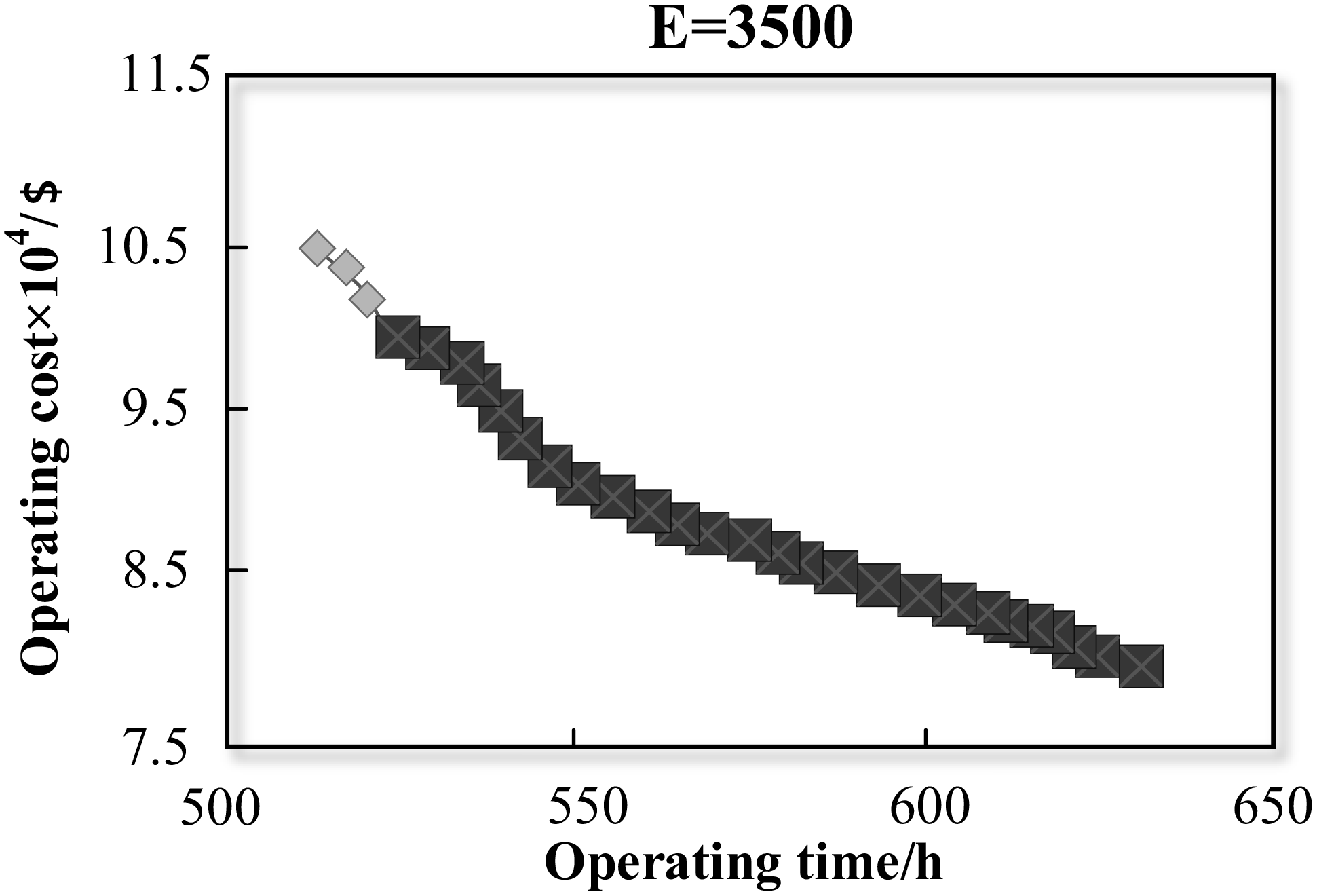
Modeling results at carbon emissions constraint III (E = 3,500).
Figure 17
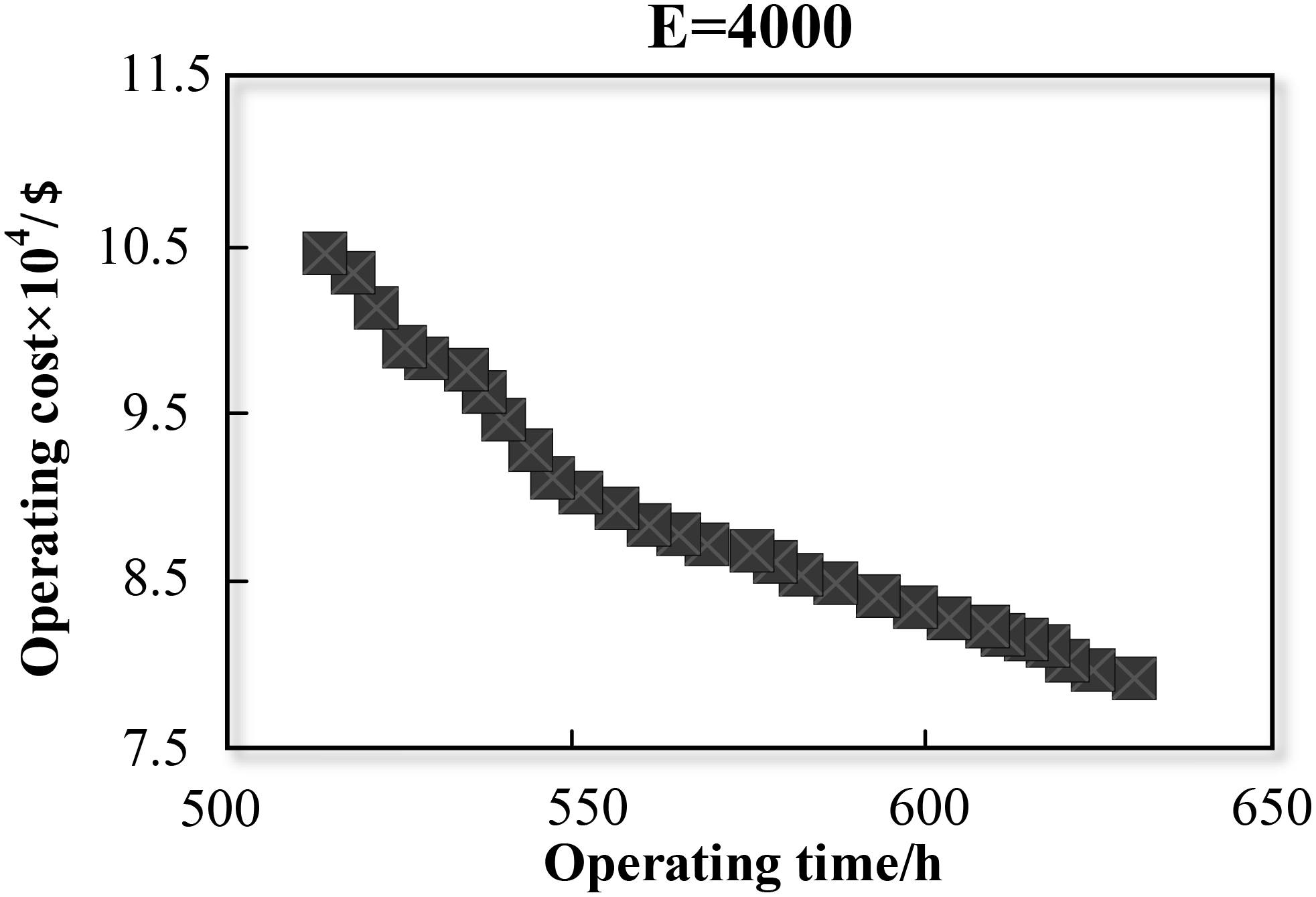
Modeling results at carbon emissions constraint IV (E = 4,000).
When the value of E is equal to 2,500 kg, the size of the Pareto set is four. The four solutions have the common characteristics of low operating cost and high operating time. The most suitable mode of transport for these characteristics should be sea transport. At the same time, sea transport is the most environmental one among all modes of transport. Thus, we can see that the results from our study are consistent with reality. With the relaxation on emission constraint, the number of Pareto solutions increases gradually. When the value of E reaches 4,000 kg, we can get all the solutions on the Pareto frontier curve. This means that when the constraint is more than 4,000 kg, it has no influence on the solution space.
(2) Sensitivity analysis of time windows
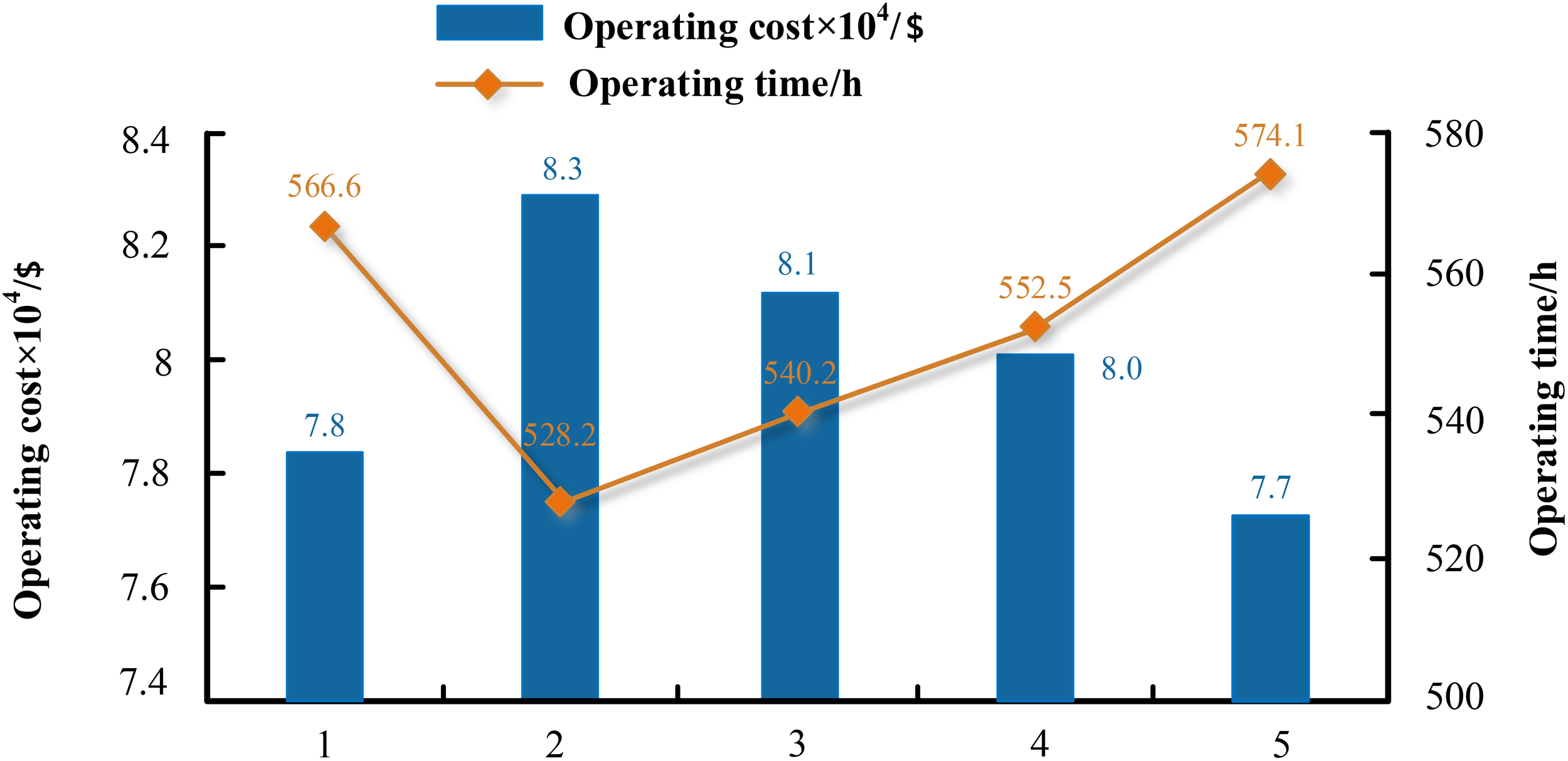
In this section, we present the comparative analysis with five different time windows. These time windows are 24, 36, 48, 60, and 72 h, respectively (labeled 1–5 in the horizontal axis of Figure 18). The optimal schemes for the five time windows are shown in Table 15. The optimal values of the objectives with these five are shown in Figure 18.
Figure 18
Comparison of results under different time window constraints.
Table 15
| Number | Time window/h | Transport route | Transport mode |
|---|---|---|---|
| 1 | 24 | 1-2-9-14-21-22-23 | 5-5-4-4-2-2 |
| 2 | 36 | 1-2-8-15-21-22-23 | 1-1-4-4-2-1 |
| 3 | 48 | 1-2-8-15-21-22-23 | 2-1-4-4-2-1 |
| 4 | 60 | 1-2-8-14-21-22-23 | 2-2-4-4-2-1 |
| 5 | 72 | 1-2-10-15-21-22-23 | 5-5-4-4-2-1 |
Transport schemes with different time window constraints.
As we can see from Table 15, different time windows will possibly lead to different optimal transport schemes, which changes the operating time and cost. Normally speaking, when the time window is relatively narrow, we will have to use a faster mode to arrive at the station before a liner/train leaves. However, if the time window is so narrow that no matter what kind of mode we use, we cannot arrive at the station and wait for the next schedule, then it will be a wiser decision to choose a relatively economical way to fulfill the transport task. This explains the phenomena in Figure 18: although case 1 has the narrowest time window, the optimal operating time is the highest, but the optimal operating cost is the lowest except for case 5. Of course, when the time window is relatively wide, it is best to choose a slow approach, so that we can catch up with the schedule and reduce the operating cost at the same time.
(3) Sensitivity analysis of regret values of p
The aim for setting p in the robust model is to ensure that the objective value of the feasible solution X under any scenario shall not exceed the (1+p) times of the optimal objective value. That is to say, the relative regret value under any scenario should not exceed p. By changing the value of this parameter, we can observe its influence on the result. Compared with the complete worst-case optimization, this model is more feasible in practical applications, and the sensitivity analysis (Table 16) verifies the adjustment effect of parameter p on the solution space.
Table 16
| Number | Value of p | Transport route | Transport mode | Operating cost/$ | Operating time/h | Size of the Pareto solution |
|---|---|---|---|---|---|---|
| 1 | 0.6 | 1-2-10-14-21-22-23 | 5-2-4-4-2-2 | 80,070.3 | 561.4 | 43 |
| 2 | 0.5 | 1-2-8-15-21-22-23 | 2-1-4-4-2-1 | 81,319.7 | 540.2 | 29 |
| 3 | 0.4 | 1-2-9-15-21-22-23 | 1-1-4-4-2-1 | 83,056.1 | 526.7 | 12 |
| 4 | 0.3 | —— | —— | —— | —— | —— |
Comparison results with the change of the regret value.
It can be seen from Table 16 that with the change of p, the optimal scheme and size of the Pareto solutions change accordingly. The influence of p on the size of the Pareto solutions is extremely great. That is because for the bi-objective model, we have to satisfy the requirements from both objectives, which narrows the solution spaces to a large extent. Thus, when the value of p is lower than 40%, the size of the solution is empty because of the strict constraint. Thus, it is necessary to set a suitable value of parameter p.
6 Conclusions
The transportation time, cost, and transshipment operation time in the Eurasian container multimodal transportation network are subject to stochastic fluctuations due to factors such as fuel price volatility and international market sentiment. To address these uncertainties, this paper establishes a multi-objective P-robust optimization model that considers uncertain factors, multiple transport corridors, and carbon emission constraints. The model aims to determine the optimal Eurasian container multimodal transportation route. An empirical study using the case of Nanjing to Berlin is conducted to validate the proposed robust model and algorithm. We analyze the impact of carbon emission constraints, time windows, and regret values on the optimal solutions. The P-regret framework offers a practical solution for real-world transportation planning, where stakeholders require both cost/time efficiency and robustness against parameter fluctuations. By bounding relative regret, the model ensures stable performance across diverse scenarios while allowing decision-makers to adjust risk tolerance via the parameter p.
In addition to the above contributions, this study has several broader implications. For practitioners, the proposed model offers a practical tool for optimizing transportation routes under uncertain conditions, helping to reduce costs, improve time efficiency, and comply with environmental regulations. This can lead to better resource allocation, enhanced supply chain resilience, and reduced carbon emissions, which are crucial for sustainable development in the logistics industry. For policymakers, the findings highlight the importance of considering uncertainty and environmental factors in transportation planning, providing a basis for formulating regulations and strategies that promote sustainable transportation practices.
Future research directions may focus on the optimization of multimodal routes considering the coordinated scheduling of full and empty containers. This could further enhance the efficiency and sustainability of container multimodal transportation networks. At the same time, in future work, we will consider introducing real network data such as port logistics and cross-border transportation for actual data set verification. We will develop and run the NSGA-II framework to deal with larger-scale problems, conduct more in-depth analysis of the computational efficiency and quality of algorithms, and perform distributed computing optimization. Additionally, future studies could explore the application of the proposed model in other regions or transportation modes, further validate its robustness under different scenarios, and investigate the potential of combining it with advanced technologies such as AI and big data analytics. Overall, this study contributes to both the academic community and industry practitioners by providing a comprehensive approach to addressing the challenges in Eurasian container multimodal transportation.
Statements
Data availability statement
The original contributions presented in the study are included in the article/supplementary material. Further inquiries can be directed to the corresponding author.
Author contributions
QX: Conceptualization, Writing – original draft, Writing – review & editing, Funding acquisition. XH: Data curation, Formal Analysis, Validation, Writing – review & editing. WZ: Investigation, Writing – review & editing. HZZ: Validation, Writing – review & editing. HPZ: Investigation, Methodology, Software, Writing – original draft. ZJ: Conceptualization, Project administration, Supervision, Writing – original draft, Writing – review & editing.
Funding
The author(s) declare that financial support was received for the research and/or publication of this article. This research is partially supported by the Natural Science Foundation of China (52362055) and the Guangxi Science and Technology Major Program (Grant No. AA23062053).
Conflict of interest
Author HPZ was employed by the company Haier Digital Technology Qingdao Co., Ltd.
The remaining authors declare that the research was conducted in the absence of any commercial or financial relationships that could be construed as a potential conflict of interest.
Generative AI statement
The author(s) declare that no Generative AI was used in the creation of this manuscript.
Publisher’s note
All claims expressed in this article are solely those of the authors and do not necessarily represent those of their affiliated organizations, or those of the publisher, the editors and the reviewers. Any product that may be evaluated in this article, or claim that may be made by its manufacturer, is not guaranteed or endorsed by the publisher.
References
1
Almasi M. H. Sadollah A. Oh Y. Kim D. K. Kang S. (2018). Optimal coordination strategy for an integrated multimodal transit feeder network design considering multiple objectives. Sustainability10, 734. doi: 10.3390/su10030734
2
Baak W. Goerigk M. Kasperski A. Zieliski P. (2025). Robust min-max (regret) optimization using ordered weighted averaging. Eur. J. Operational Res.322, 171–181. doi: 10.1016/j.ejor.2024.10.028
3
Campuzano G. Lalla-Ruiz E. Mes M. (2025). The two-tier multi-depot vehicle routing problem with robot stations and time windows. Eng. Appl. Artif. Intell.147, 110258. doi: 10.1016/j.engappai.2025.110258
4
Cao W. J. Wang X. J. Li J. Zhang Z. W. Cao Y. H. Feng Y. W. (2024). A novel integrated method for heterogeneity analysis of marine accidents involving different ship types. Ocean Eng.312, 119295. doi: 10.1016/j.oceaneng.2024.119295
5
Chen X. H. Hu X. H. Liu H. B. (2024). Low-carbon route optimization model for multimodal freight transport considering value and time attributes. Socio-Economic Plann. Sci.96, 102108. doi: 10.1016/j.seps.2024.102108
6
Cheng Z. L. Zhao L. J. Li H. Y. (2022). Key factors that influence the performance of China Railway express operations: case studies of ten lines in China. Int. J. Shipping Transport Logistics14, 395–431. doi: 10.1504/IJSTL.2022.123714
7
Deb K. Pratap A. Agarwal S. Meyarivan T. (2002). A fast and elitist multiobjective genetic algorithm: NSGA-II. IEEE Trans. Evolutionary Comput.6, 182–197. doi: 10.1109/4235.996017
8
Deng Y. J. Zhu X. N. (2019). “Research on transportation organization modes for China railway express,” in 2018 International Seminar On Computer Science And Engineering Technology. J. Phys.: Conf. Ser.1176 (4), 042006. doi: 10.1088/1742-6596/1176/4/042006
9
Derpich I. Duran C. Carrasco R. Moreno F. Fernandez-Campusano C. Espinosa-Leal L. (2024). Pursuing optimization using multimodal transportation system: A strategic approach to minimizing costs and CO2 emissions. J. Of Marine Sci. And Eng.12, 976. doi: 10.3390/jmse12060976
10
Eurostat (2024). China-europe trade surge: A decade of growth following landmark infrastructure initiatives. Available online at: https://ec.europa.eu/eurostat (Accessed 2024).
11
Graff L. K. Flanigan K. A. Qian S. (2024). Constructing a routable multimodal, multi-cost, time-dependent network model with all emerging mobility options: Methodology and case studies. Transportation Res. Part E: Logistics Transportation Rev.192, 103757. doi: 10.1016/j.tre.2024.103757
12
Grisales-Noreña L. F. Cortés-Caicedo B. Montoya O. D. Bolaños R. I. Moreno C. A. M. (2024). Nonlinear programming for BESS operation for the improvement of economic, technical and environmental indices by considering grid-connected and stand-alone networks: An application to the territory of Colombia. J. Energy Storage98, 112856. doi: 10.1016/j.est.2024.112856
13
Guo L. M. Du J. Zheng J. F. He N. (2023). Integrated planning of feeder route selection, schedule design, and fleet allocation with multimodal transport path selection considered. J. Of Marine Sci. And Eng.11, 1445. doi: 10.3390/jmse11071445
14
Guo L. Q. Jiang C. M. Hou W. L. Ng A. K. Y. Shi Q. (2024b). International multimodal transport connectivity assessment of multimodal transport from mainland China to Europe. Transportation Res. Part E: Logistics Transportation Rev.186, 103564. doi: 10.1016/j.tre.2024.103564
15
Guo J. W. Wang W. Guo J. Y. D’Ariano A. Bosi T. Zhang Y. X. (2024a). An instance-based transfer learning model with attention mechanism for freight train travel time prediction in the China-Europe railway express. Expert Syst. Appl.251, 123989. doi: 10.1016/j.eswa.2024.123989
16
He S. C. Xie H. B. Feng Y. W. (2024). The optimization of fleet deployment for container liner shipping under the carbon tax and energy efficiency operation indicator. Asce-asme J. Of Risk And Uncertainty In Eng. Syst. Part A-Civil Eng.10, 04024056. doi: 10.1061/AJRUA6.RUENG-1354
17
Hou J. (2018). “Dynamic multi-objective optimization problem of container intermodal transport: an empirical analysis on the belt and road initiative of China,” in Proceedings of the 3rd International Conference on Electrical and Information Technologies for Rail Transportation (EITRT) 2017 Transportation. SpringerSingapore, 679–688. doi: 10.1007/978-981-10-7989-4_69
18
Hou Y. J. Liao X. J. Chen G. Z. Chen Y. (2025). Co-Evolutionary NSGA-III with deep reinforcement learning for multi-objective distributed flexible job shop scheduling. Comput. Industrial Eng.203, 110990. doi: 10.1016/j.cie.2025.110990
19
Huang C. Sun H. B. Liu C. J. Zhang X. Q. Gao T. H. Tian J. (2025). Research on container multimodal transportation multi-objective path optimization from hinterlands to shanghai port. IEEE Access13, 32794–32807. doi: 10.1109/access.2025.3532387
20
Im H. Yu J. Lee C. (2021). Truck appointment system for cooperation between the transport companies and the terminal operator at container terminals. Appl. Sciences-Basel11, 168. doi: 10.3390/app11010168
21
Kim M. Hiroyasu T. Miki M. Watanabe S. “SPEA2+: Improving the performance of the strength pareto evolutionary algorithm 2” in: 8th International Conference on Parallel Problem Solving from Nature. (Springer Verlag), 742–751. doi: 10.1007/978-3-540-30217-9_75
22
Li X. Y. Xie C. Bao Z. Y. (2022). A multimodal multicommodity network equilibrium model with service capacity and bottleneck congestion for China-Europe containerized freight flows. Transportation Res. Part E: Logistics Transportation Rev.164, 102786. doi: 10.1016/j.tre.2022.102786
23
Lim H. Lee G. M. Singgih I. K. (2021). Multi-depot split-delivery vehicle routing problem. IEEE Access9, 112206–112220. doi: 10.1109/ACCESS.2021.3103640
24
Lin Q. Z. Tang C. Y. Ma Y. P. Du Z. H. Li J. Q. Chen J. Y. et al . (2017). A novel adaptive control strategy for decomposition-based multiobjective algorithm. Comput. Operations Res.78, 94–107. doi: 10.1016/j.cor.2016.08.012
25
Liu M. Xin X. Wang X. Zhang T. Chen K. (2025). Dual-channel slot sales strategy for container liner shipping companies with blockchain technology adoption. Transport Policy162, 200–220. doi: 10.1016/j.tranpol.2024.12.006
26
Liu C. C. Zhou Y. J. Yang Z. Z. Li Y. M. Li T. (2024). Optimizing the scheduling scheme for NSR/SCR tramp vessel shipping between Asia and Europe. Ocean Eng.304, 117747. doi: 10.1016/j.oceaneng.2024.117747
27
Liyanage S. Dia H. Duncan G. Abduljabbar R. (2024). Evaluation of the impacts of on-demand bus services using traffic simulation. Sustainability16, 8477. doi: 10.3390/su16198477
28
Lu M. Chen Y. Lu Y. (2018). The competition and cooperation spatial pattern between rail way transport and shipping in China under the Belt and Road Initiative. Geographical Res.37, 404–418. doi: 10.11821/dlyj201802013
29
Lv L. L. Shen W. M. (2023). An improved NSGA-II with local search for multi-objective integrated production and inventory scheduling problem. J. Manufacturing Syst.68, 99–116. doi: 10.1016/j.jmsy.2023.03.002
30
Ma Y. Li B. Huang W. T. Fan Q. Q. (2023c). An improved NSGA-II based on multi-task optimization for multi-UAV maritime search and rescue under severe weather. J. Marine Sci. Eng.11, 781. doi: 10.3390/jmse11040781
31
Ma J. C. Wang X. F. Yang K. Jiang L. J. (2023b). Uncertain programming model for the cross-border multimodal container transport system based on inland ports. Axioms12 (2), 132. doi: 10.3390/axioms12020132
32
Ma H. P. Zhang Y. J. Sun S. Y. Liu T. Shan Y. (2023a). A comprehensive survey on NSGA-II for multi-objective optimization and applications. Artif. Intell. Rev.56, 15217–15270. doi: 10.1007/s10462-023-10526-z
33
National Bureau of Statistics of China (2024). European Market Share: A Key Destination for Chinese Exports. Available online at: https://www.stats.gov.cn (Accessed 2024).
34
Noruzi M. Naderan A. Zakeri J. A. Rahimov K. (2023). A robust optimization model for multi-period railway network design problem considering economic aspects and environmental impact. Sustainability15, 5022. doi: 10.3390/su15065022
35
Pak N. Nahavandi N. Bagheri B. (2022). Designing a multi-objective green supply chain network for an automotive company using an improved meta-heuristic algorithm. Int. J. Environ. Sci. Technol.19, 3773–3796. doi: 10.1007/s13762-021-03521-w
36
Prakash S. Mehta U. Sharma B. (2024). Artificial intelligence-driven multimodal route planning: addressing dynamic unavailability and disruptions. IEEE Access12, 172088–172100. doi: 10.1109/ACCESS.2024.3498863
37
Qi C. (2024). Multi-objective optimization-based algorithm for selecting the optimal path of rural multi-temperature zone cold chain dynamic logistics intermodal transportation. Int. J. Comput. Intell. Syst.17, 224. doi: 10.1007/s44196-024-00616-3
38
Raad N. G. Swain C. Ayantayo A. Yang B. Rajendran S. (2024). Hybrid regret-based p-robust and distributionally robust optimization models for electric vehicle charging station network design. Comput. Industrial Eng.198, 110709. doi: 10.1016/j.cie.2024.110709
39
Shen H. C. Tzu F. M. Lin C. Yeh C. K. Huang W. Y. Pu H. P. et al . (2022). Verification of Fuel Consumption and Carbon Dioxide Emissions under Sulfur Restriction Policy during Oceanographic Navigation. Appl. Sciences-Basel12, 9857. doi: 10.3390/app12199857
40
Singgih I. K. Singgih M. L. (2024). Regression machine learning models for the short-time prediction of genetic algorithm results in a vehicle routing problem. World Electric Vehicle J.15, 308. doi: 10.3390/wevj15070308
41
Tyurin A. Stoianov A. (2019). “Improving the mining enterprise productivity based on probabilistic nature of the solid minerals extraction and transportation,” in E3S Web of Conferences, EDP Sciences, 105, 01038. doi: 10.1051/e3sconf/201910501038
42
Wang Y. Gou M. Luo S. Fan J. Wang H. (2025a). The multi-depot pickup and delivery vehicle routing problem with time windows and dynamic demands. Eng. Appl. Artif. Intell.139, 109700. doi: 10.1016/j.engappai.2024.109700
43
Wang N. Yan B. Wu D. Wu N. (2017). The spatio-temporal pattern of China-EU shipping route under the background of Arctic navigation. J. Economic Geography37, 9–16. doi: 10.15957/j.cnki.jjdl.2017.12.002
44
Wang Z. J. Zhang D. Z. Tavasszy L. Fazi S. (2025b). The hierarchical multimodal hub location problem for cross-border logistics networks considering multiple capacity levels, congestion and economies of scale. Transportation Res. Part E-Logistics Transportation Rev.196, 103972. doi: 10.1016/j.tre.2025.103972
45
Xiang Z. L. Xin X. Zhang T. Chen K. Liu M. H. (2025). Asia-Europe liner shipping network design model considering Arctic route and black carbon tax. Ocean Coastal Manage.261, 107492. doi: 10.1016/j.ocecoaman.2024.107492
46
Xiao G. N. Cui W. Y. (2023). Evolutionary game between government and shipping enterprises based on shipping cycle and carbon quota. Front. Marine Sci.10. doi: 10.3389/fmars.2023.1132174
47
Xiao G. N. Pan L. Lai F. B. (2025). Application, opportunities, and challenges of digital technologies in the decarbonizing shipping industry: a bibliometric analysis. Front. Marine Sci.12. doi: 10.3389/fmars.2025.1523267
48
Xin X. Zhang T. Wang X. L. He F. Wu L. X. (2025). Risk-averse distributionally robust optimization for construction waste reverse logistics with a joint chance constraint. Comput. Operations Res.173, 106829. doi: 10.1016/j.cor.2024.106829
49
Xin-gang Z. Wenjie L. Wei W. Shuran H. (2023). Impact of carbon emissions trading on green total factor productivity of China’s power industry: A green technology innovation perspective. Environ. Impact Assess. Rev.99, 015906. doi: 10.1016/j.eiar.2023.107040
50
Xu L. Shen C. Chen J. (2024a). The impact of the Maritime Silk Road Initiative on the carbon intensity of the participating countries. Maritime Economics Logistics1–19. doi: 10.1057/s41278-024-00295-z
51
Xu L. Yang Z. H. Chen J. H. Zou Z. Y. (2023). Impacts of the COVID-19 epidemic on carbon emissions from international shipping. Marine Pollution Bull.189, 114730. doi: 10.1016/j.marpolbul.2023.114730
52
Xu L. Yang Z. H. Chen J. H. Zou Z. Y. Wang Y. (2024b). Spatial-temporal evolution characteristics and spillover effects of carbon emissions from shipping trade in EU coastal countries. Ocean Coastal Manage.250, 107029. doi: 10.1016/j.ocecoaman.2024.107029
53
Xu Q. Zhong Y. Deng H. Wang X. Chen X. (2024c). Scheduling on tractor and trailer transportation considering the influence of disrupted events based on the contract net and simulated annealing algorithm. Digital Transportation Saf.3, 155–168. doi: 10.48130/dts-0024-0014
54
Yang D. Jiang L. P. Ng A. K. Y. (2018). One Belt one Road, but several routes: A case study of new emerging trade corridors connecting the Far East to Europe. Transportation Res. Part A: Policy Pract.117, 190–204. doi: 10.1016/j.tra.2018.08.001
55
Yang J. H. Liang D. F. Zhang Z. W. Wang H. F. Bin H. (2024). Path optimization of container multimodal transportation considering differences in cargo time sensitivity. Transportation Res. Record2678, 1279–1292. doi: 10.1177/03611981241243077
56
Yi J. H. Deb S. Dong J. Y. Alavi A. H. Wang G. G. (2018). An improved NSGA-III algorithm with adaptive mutation operator for Big Data optimization problems. Future Generation Comput. Systems-the Int. J. Escience88, 571–585. doi: 10.1016/j.future.2018.06.008
57
Yilmaz B. G. Yilmaz O. F. Akçali E. Çevikcan E. (2025). Seru scheduling problem with lot streaming and worker transfers: A multi-objective approach. Comput. Operations Res.177, 106967. doi: 10.1016/j.cor.2024.106967
58
Zeinab Aliahmadi S. Jabbarzadeh A. Hof L. A. (2025). A multi-objective optimization approach for sustainable and personalized trip planning: A self-adaptive evolutionary algorithm with case study. Expert Syst. Appl.261, 125412. doi: 10.1016/j.eswa.2024.125412
59
Zhang T. Cheng J. Zou Y. B. (2024). Multimodal transportation routing optimization based on multi-objective Q-learning under time uncertainty. Complex Intelligent Syst.10, 3133–3152. doi: 10.1007/s40747-023-01308-9
60
Zhang Y. Z. Guo Y. A. Huang Y. Ge S. R. (2025). A low-carbon scheduling method based on improved ant colony algorithm for underground electric transportation vehicles. Complex Intelligent Syst.11, 166. doi: 10.1007/s40747-024-01775-8
61
Zhang X. Zhang W. Lee P. T. W. (2020). Importance rankings of nodes in the China Railway Express network under the Belt and Road Initiative. Transportation Res. Part A: Policy Pract.139, 134–147. doi: 10.1016/j.tra.2020.07.003
62
Zhao L. J. Zhao Y. Hu Q. M. Li H. Y. Stoeter J. (2018). Evaluation of consolidation center cargo capacity and loctions for China railway express. Transportation Res. Part E: Logistics Transportation Rev.117, 58–81. doi: 10.1016/j.tre.2017.09.007
63
Zhou Y. T. Li Z. F. Duan W. (2024). Exploring the dynamic impact of the Northern Sea Route on China-Europe multimodal transportation competition in the context of the Belt and Road Initiative. Ocean Coastal Manage.257, 107346. doi: 10.1016/j.ocecoaman.2024.107346
64
Zhu L. Ding T. Liu Z. F. (2024). Reverse logistics network design for medical waste disposal under the scenario of uncertain proposal demand. Sustainability16, 2996. doi: 10.3390/su16072996
Summary
Keywords
Container multimodal transportation, robust optimization, multi-objective model, NSGA-II, carbon emission
Citation
Xu Q, Huang X, Zhang W, Zhao H, Zhang H and Jin Z (2025) Eurasian container intermodal transportation network: a robust optimization with uncertainty and carbon emission constraints. Front. Mar. Sci. 12:1576006. doi: 10.3389/fmars.2025.1576006
Received
13 February 2025
Accepted
07 April 2025
Published
20 May 2025
Volume
12 - 2025
Edited by
Lang Xu, Nanyang Technological University, Singapore
Reviewed by
Ivan Kristianto Singgih, Korea University, Republic of Korea
Guangnian Xiao, Shanghai Maritime University, China
Zhong Shuo Chen, Xi’an Jiaotong-Liverpool University, China
Updates
Copyright
© 2025 Xu, Huang, Zhang, Zhao, Zhang and Jin.
This is an open-access article distributed under the terms of the Creative Commons Attribution License (CC BY). The use, distribution or reproduction in other forums is permitted, provided the original author(s) and the copyright owner(s) are credited and that the original publication in this journal is cited, in accordance with accepted academic practice. No use, distribution or reproduction is permitted which does not comply with these terms.
*Correspondence: Zhihong Jin, jinzhihong@dlmu.edu.cn
Disclaimer
All claims expressed in this article are solely those of the authors and do not necessarily represent those of their affiliated organizations, or those of the publisher, the editors and the reviewers. Any product that may be evaluated in this article or claim that may be made by its manufacturer is not guaranteed or endorsed by the publisher.