Abstract
Nitrate is a critical limiting nutrient that significantly influences marine primary productivity and carbon sequestration. However, three-dimensional observation and reconstruction of oceanic nitrate remain constrained by the scarcity of in-situ data and limited spatial coverage. To address the challenge of limited observational labels hindering the development of global deep learning models for marine three-dimensional estimation, this study proposes a novel deep learning framework that utilizes underwater signals for label augmentation, thereby reducing the uncertainty in three-dimensional nitrate estimation. Initially, we employ a Bayesian neural network, utilizing multiple subsurface parameters from Biogeochemical-Argo (BGC-Argo) measurements to generate virtual nitrate labels with quantified uncertainty. These augmented labels are then assimilated into a U-Net-based model, greatly expanding the training dataset and further integrating sea surface environmental variables for comprehensive three-dimensional reconstruction. The proposed uncertainty-weighted loss function refines model training, balancing the quality and training impact of both observed and augmented labels. Quantitative evaluations using BGC-Argo and cruise measurement data demonstrate notable improvements in spatial and temporal generalization, with RMSE reductions of approximately 15% and 28%, respectively, particularly in under-sampled areas and complex upper ocean regions. This research framework offers a promising solution for oceanic three-dimensional data reconstruction in the absence of supervised data and has the potential to be coupled with various marine parameters and reconstruction models, providing deeper insights into the spatiotemporal variations of marine environments.
1 Introduction
Nitrate, as one of the key limiting nutrients in marine ecosystems, plays a crucial role in the marine environment (Bristow et al., 2017; Chen et al., 2023). It directly regulates marine primary productivity, thereby influencing the ocean’s carbon sequestration capacity and its response to climate change (Friedlingstein et al., 2020; Eppley and Peterson, 1979; Gregg et al., 2003; Rafter et al., 2017). Therefore, a thorough analysis and systematic monitoring of the spatial and temporal distribution of nitrate in the ocean, as well as its dynamic variations, is an essential foundation for studying marine ecosystems, the global carbon cycle, and climate change.
However, observing marine nitrate remains fraught with numerous technical challenges. Due to the weak optical signature of nitrate and its complex, nonlinear relationship with environmental factors, remote sensing inversion has yet to overcome technological bottlenecks (Chen et al., 2023; Sathyendranath et al., 1991). As a result, standardized global-scale data products are still lacking (Yu et al., 2022). Moreover, the role of nitrate in the ocean is not confined to the surface; its three-dimensional (3D) spatial distribution and dynamic evolution processes remain significant gaps in our understanding. Although platforms like Biogeochemical Argo (BGC-Argo) and shipborne observations have provided invaluable in situ data for 3D nitrate monitoring (Claustre et al., 2020; Lavigne et al., 2015; Nittis et al., 2007), their limited spatial and temporal coverage hinders continuous, large-scale assessments (Yang et al., 2022). This limitation in observational capability hinders our ability to fully comprehend the distribution characteristics of nitrate at various depths and regions of the ocean, which in turn affects the accurate assessment of marine ecosystems. Consequently, filling these data gaps and constructing a 3D distribution model of marine nitrate has become a pivotal scientific task in the study of marine environmental and ecological changes.
The estimation methods for 3D nitrate provide new avenues to bridge this research gap. By modeling biogeochemical processes, 3D continuous numerical model products can be generated (Baretta et al., 1995; Bruggeman and Bolding, 2014; Holt et al., 2012; Kay and Butenschön, 2018). Although these models are effective at capturing large-scale changes in the ocean, they still face challenges in accurately representing the complex nonlinear relationships and small-scale variations inherent in simulating highly nonlinear ocean processes (Yang et al., 2024; Tian et al., 2022). In contrast, deep learning methods have demonstrated significant development potential (Yuan et al., 2020; Feng et al., 2024). By integrating extensive remote sensing observations and high-precision in situ measurements, these methods leverage the capacity of neural networks to model complex relationships, offering the possibility of achieving higher accuracy (Chang et al., 2013; Pan et al., 2018).
Deep learning estimation models for 3D nitrate and other parameters in the ocean can be categorized into two main types: local models and global models, based on their structure. Local models rely on ocean surface or underwater environmental parameters at individual latitude and longitude coordinates to independently predict vertical profiles (Hu et al., 2023; Tian et al., 2022; Bittig et al., 2018). For instance, Wang et al. (2023) utilized a regional deep neural network (DNN) to estimate nitrate concentrations in the Northwest Pacific. Similar supervised learning methods based on multilayer perceptrons (MLP) have also been applied to reconstruct water column bio-optical and biogeochemical parameters using remote sensing and BGC-Argo data (Fourrier et al., 2020; Sauzède et al., 2017). These local models have similarly achieved success in estimating typical marine environmental parameters such as temperature, salinity, and chlorophyll. However, local models are limited to input features from single coordinate points, failing to fully harness the potential of neural networks to capture large-scale spatial-temporal patterns. Given that the relationship between nitrate and environmental variables exhibits significant spatiotemporal variability, local models face substantial challenges in estimating 3D nitrate.
By contrast, global models can incorporate continuous spatiotemporal features (e.g., convolutional neural networks (CNN) or Transformers) and leverage advanced network architectures to capture intricate spatiotemporal relationships, thereby attaining stronger generalization performance (Buongiorno Nardelli, 2020; Qi et al., 2022; Smith et al., 2023; Cheng et al., 2025; Su et al., 2021; Gao et al., 2024). For example, Yang et al. (2024); Zhang et al. (2024) successfully reconstructed the 3D nitrate structure of the Indian Ocean based on surface data using two artificial intelligence networks. The Transformer model developed enabled the estimation of the ENSO coefficient through long temporal sequences and broad spatial-temporal inputs (Zhou and Zhang, 2023). However, when training global models, the limited availability of nitrate in situ data hampers the ability to provide sufficient label matching for large-scale spatiotemporal features, resulting in many spatiotemporal characteristics not effectively contributing to model fitting. To overcome this limitation, the aforementioned studies turned to numerical model products as supervised training data. Yet, the inherent uncertainty in these products limits the accuracy of the model fitting, which could lead to discrepancies between the reconstructed results and actual conditions, thereby affecting the model’s accuracy and stability in practical applications (Tian et al., 2022).
From the above analysis, a key bottleneck in 3D nitrate estimation is the limited availability of in situ measurement labels, which narrows the training scope and hinders effective data utilization in both local and global models. To mitigate this issue, we propose an innovative approach for nitrate 3D reconstruction by integrating Bayesian neural networks (BNN) with deep learning models, addressing both data sparsity and uncertainty quantification. Specifically, we first employ the Bayesian neural network to model the relationship between other sub-surface variables and nitrate concentration, generating augmented labels to compensate for the lack of observational data, while also quantifying the uncertainty of these labels through the BNN. Subsequently, we combine the augmented labels with the observed ones, using them as supervisory signals to train a spatiotemporal continuous deep learning model (such as UNet). During the training process, the model not only accounts for spatial continuity but also incorporates uncertainty quantification into the loss function, reducing the impact of label uncertainty on the model’s results, thereby significantly enhancing the precision of 3D nitrate reconstruction.
2 Materials and methods
2.1 Study area
This study selects the Mediterranean Sea (MED) as a typical research area, with the study range spanning from 6°W to 37°E longitude and from 30°N to 46°N latitude. As a semi-enclosed sea, The MED not only faces the impact of active human activities but also exhibits the characteristic of low nutrient levels that decrease progressively from west to east. The region is equipped with a relatively dense BGC-Argo observation network, providing an ideal setting for comparing and evaluating the effectiveness of label augmentation.
2.2 Data
This study utilizes two types of in situ data from the BGC-Argo and GLODAPv2 databases, along with three types of Sea surface environmental data. BGC-Argo (https://argo.ucsd.edu, https://www.ocean-ops.org/) is a sensor-equipped profiling buoy network, representing one of the most promising ocean vertical observation technologies. BGC-Argo is capable of monitoring multiple biogeochemical and environmental variables, including nitrate, and has collected 283,482 nitrate measurements within the study area, while also synchronously observing numerous other variables (Table 1), providing a comprehensive dataset of underwater variables (Johnson et al., 2024, 2021). Nitrate concentration is measured using ultraviolet absorption spectroscopy (Johnson et al., 2024), with an average accuracy of ±0.5µmol · kg−1 (Johnson et al., 2021, 2017; Mignot et al., 2019). Furthermore, the GLODAPv2 database (https://www.ncei.noaa.gov/access/ocean-carbon-acidification-data-system/oceans/GLODAPv2_2022/) offers a unified, calibrated open-ocean data product on inorganic carbon and carbon-related variables (Lauvset et al., 2022, 2021; Olsen et al., 2020), used for independently validating the model’s predictive performance.
Table 1
| Group | Observation Depth Range (m) | Variable | Number of Synchronous Observations with Nitrate |
Number of Asynchronous Observations with Nitrate |
Pearson Correlation Coefficient with Nitrate | Mutual Information Coefficient with Nitrate |
|---|---|---|---|---|---|---|
| 0-2000 | Nitrate | 283482 | ||||
| 1 | 0-2000 | TEMP | 281480 | 16361956 | -0.71 | 5.61 |
| PSAL | 259693 | 15429530 | -0.183 | 5.608 | ||
| 2 | 0-300 | CHL | 262719 | 4510059 | -0.43 | 3.056 |
| FLUO | 253558 | 4101896 | -0.423 | 3.17 | ||
| BBP700 | 250341 | 4005839 | -0.336 | 5.448 | ||
| 3 | 0-300 | LGHT | 117845 | 2453057 | -0.281 | 9.007 |
| Ed380 | 117845 | 2453061 | -0.258 | 6.665 | ||
| Ed412 | 117845 | 2453055 | -0.312 | 7.58 | ||
| Ed490 | 117845 | 2453053 | -0.359 | 8.339 | ||
| 4 | 0-2000 | DOX2 | 199387 | 2108601 | -0.833 | 7.916 |
| 5 | 0-2000 | PH | 6984 | 24924 | -0.561 | 5.558 |
Characteristics of BGC-Argo observed variables and their relationship with nitrate.
Sea surface environment variables are used as input features for the 3D reconstruction model (Yang et al., 2024; Goes et al., 1999; Pan et al., 2018; Wang et al., 2023), with a uniform resolution of monthly averages and 0.25°. The satellite-derived ocean color data come from the European Space Agency’s Globcolour project (Lavender et al., 2009) (http://globcolour.info/), including chlorophyll (Chl), photosynthetically available radiation (PAR), and Coloured dissolved materials (CDM). Meteorological driving data come from the ERA5 reanalysis dataset (Hersbach et al., 2020) (https://cds.climate.copernicus.eu/), including sea surface temperature (SST), 10 m U wind component (U10), 10 m V wind component (V10), 10 m wind speed (S10). The Copernicus Marine Service (CMEMS, https://marine.copernicus.eu/) provides ocean dynamical data, including sea surface height (SSH), mixed layer thickness (MLD), and sea surface salinity (SSS).
2.3 Research process
Figure 1 illustrates the overall workflow of this study, incorporating various data sources as described in Section 2.2. Multiple variables measured by BGC-Argo are screened and standardized. Observational samples that simultaneously measure nitrate and the required subsurface variables are input into a Bayesian Neural Network (BNN) for training (Figure 1C). Once training is complete, for observational samples where other subsurface scalar variables are measured but nitrate is not, the BNN is capable of estimating a virtual nitrate label and assessing its uncertainty. Subsequently, the measured nitrate labels from BGC-Argo and the estimated nitrate labels from the BNN are integrated into an augmented labeled dataset, using uncertainty as a weighting factor. This dataset is then subjected to binning and preprocessing to generate a 3D gridded dataset with a horizontal resolution of 0.25° and 63 depth levels, incrementally spanning from the surface to a depth of 2000 meters. The processed dataset is then matched with ocean surface environmental variable features and input into a 3D estimation network for training (Figure 1D).
Figure 1
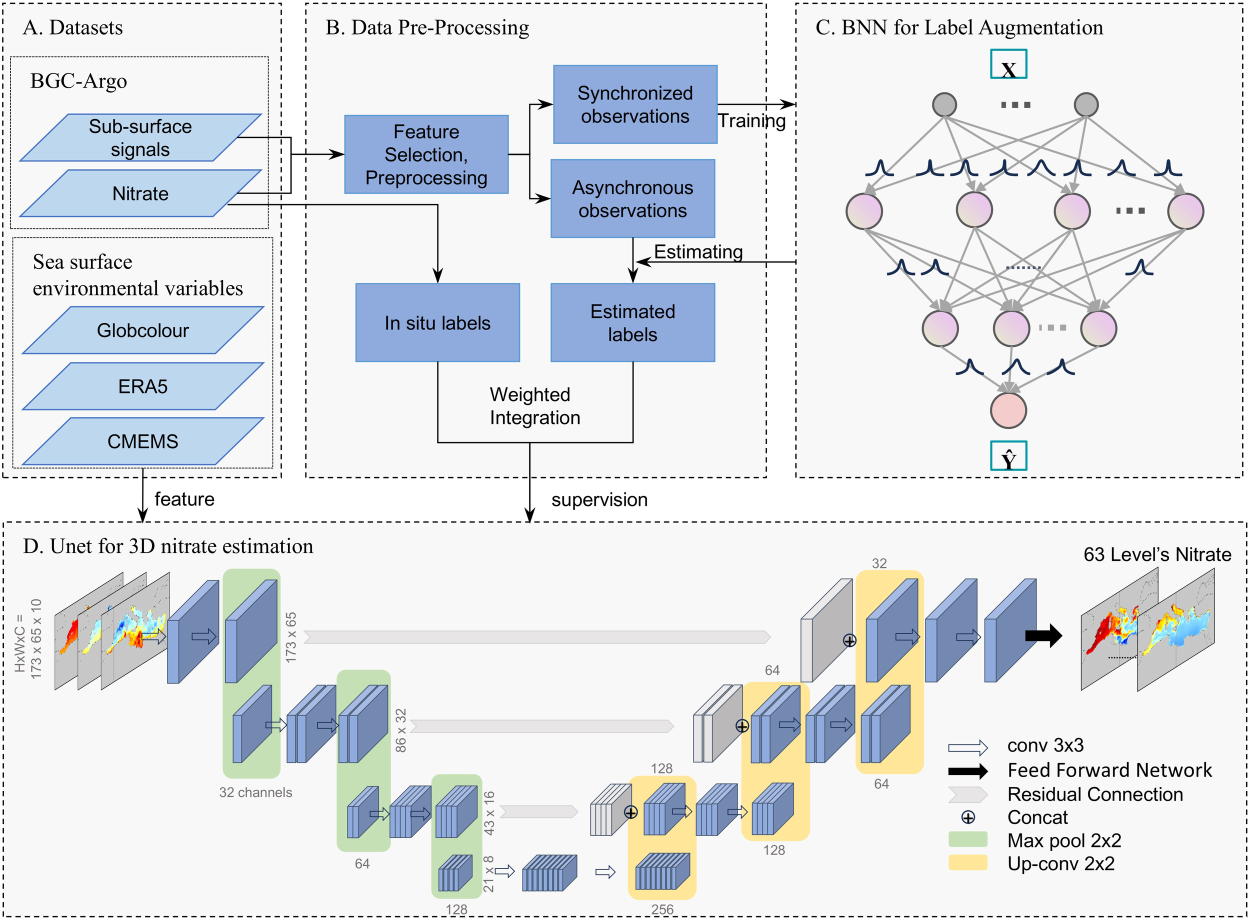
Workflow for nitrate estimation, showing (A) Datasets, (B) Data Pre-processing, (C) BNN for Label Augmentation, and (D) U-Net for 3D nitrate estimation.
2.4 Bayesian neural network for label augmentation
In the task of reconstructing 3D nitrate distributions in the ocean, the sparsity of labels is one of the key factors affecting model performance. To address this issue, this study proposes a label augmentation method based on Bayesian Neural Networks (BNN) (Blundell et al., 2015). BNNs are a deep learning models that not only make predictions but also quantify uncertainty, making it particularly useful in applications requiring probabilistic reasoning. In contrast to traditional neural networks, BNNs place a probability distribution over the weights, enabling explicit quantification of prediction uncertainty. This feature is particularly important for estimating complex nonlinear relationships in marine environments. The BNN developed in this study employs a multilayer perceptron structure, with input features including depth, temperature, salinity, chlorophyll a, and other covariates observed by BGC-Argo, and the output being nitrate concentration along with its uncertainty estimates.
In the network design, each weight is modeled as a Gaussian distribution, with parameter estimation performed through variational inference. Specifically, the network consists of three hidden layers. The first layer has neurons equal to the number of input features, the second layer contains 32 neurons, and the third layer has a single neuron, utilizing the LeakyRelu activation function. To prevent overfitting, dropout regularization (with a rate of 0.1) is applied. The core of the BNN is to learn the posterior distribution of the parameters w, rather than the point estimates used in traditional neural networks. For input data X and labels Y, Bayesian inference can be represented as Equation 1:
where, represents the prior distribution of the weights (a standard normal distribution is chosen), and is the likelihood function. Since the posterior distribution is difficult to compute directly, we employ variational inference, introducing a variational posterior distribution to approximate the true posterior distribution. Each individual prediction is modeled as a Gaussian distribution, as shown in Equation 2:
where, represents the output of the neural network, and denotes the irreducible error (aleatory uncertainty). The network is trained by minimizing the Evidence Lower Bound (ELBO) loss function to optimize the model parameters, as defined in Equation 3:
where, is the balancing factor (set to 0.1), used to adjust the relative importance of the likelihood term and the KL divergence term. In practice, variational inference is implemented through Monte Carlo dropout. For a new input , the prediction is sampled by performing forward passes (with ), and the mean and variance of the predictions are calculated as Equations 4 and 5:
Simultaneously, the uncertainty of the estimated values is computed as follows:
During the BNN training phase, we initially selected multiple BGC-Argo observation sets where nitrate and subsurface parameters were measured concurrently. The former serves as the label, and the latter as the feature. These data were standardized using Z-scores to form the dataset. The data were divided into five folds by profile, with 20% of the profiles selected as the test set and 80% as the training set. The model was trained using the Adam optimizer with an initial learning rate of 0.001 and a batch size of 64.
The BNN’s performance was evaluated on the test set by comparing the estimated values to the in-situ nitrate values, using statistical metrics including the Determination Coefficient (R2), Mean Bias Error (MBE), Mean Squared Error (MSE), Root Mean Squared Error (RMSE), Mean Absolute Error (MAE), and Median Absolute Error (MedAE).
The advantage of BNN lies in its ability to handle label uncertainty. By quantifying the uncertainty of augmented labels, it mitigates the risks posed by low-quality augmented labels during model training. Specifically, BNN reduces dependence on high-uncertainty labels when augmenting labels, thereby enhancing robustness during the training process. Furthermore, the posterior distribution of the BNN provides multiple possibilities for the augmented labels, which significantly supports the model’s generalization ability in data-sparse regions.
2.5 UNet for 3D reconstruction
This study adopts an improved UNet (Ronneberger et al., 2015) architecture for the spatial reconstruction of oceanic nitrate concentrations. Compared to profile-based local reconstruction models, the encoderdecoder structure of UNet effectively captures local and global spatial dependencies, crucial for reconstructing the spatial distribution patterns of oceanic nitrate.
The UNet architecture employed in this study follows an encoder-decoder structure optimized for capturing hierarchical features from high-dimensional spatiotemporal data. The encoder progressively compresses input features through a series of downsampling operations, capturing both localized features and broader contextual information. Each encoding step consists of two consecutive convolutional layers with a kernel size of 3×3, followed by batch normalization and LeakyReLU activation functions, enhancing the model’s ability to handle complex nonlinear relationships.
Specifically, the encoder comprises four sequential downsampling modules, each employing a maxpooling operation with a stride of 2 to reduce the spatial dimensions, resulting in increasingly abstract and condensed representations of the input data. These compressed features effectively summarize essential environmental patterns across multiple scales and depths.
The decoder symmetrically mirrors the encoder’s structure, employing transposed convolutional layers for upsampling to reconstruct detailed spatial structures. Each upsampling module restores spatial resolution and progressively integrates high-level semantic context through concatenation with corresponding encoder features via skip connections. These skip connections ensure that crucial spatial information lost during downsampling is effectively recovered, significantly improving the fidelity of nitrate concentration reconstructions.
In the decoder, each upsampling step is followed by two convolutional layers with kernel sizes of 3×3 and LeakyReLU activation functions, maintaining consistency and symmetry with the encoder. The final decoder output undergoes an additional feature integration process, implemented through a fully connected (FC) layer composed of two consecutive 1×1 convolutional layers. These convolutional layers transform the high-dimensional feature representations into nitrate concentration values at predefined vertical depth levels, yielding a comprehensive three-dimensional nitrate field.
The model inputs ocean surface environmental variables as features. The tensor contains environmental variables with dimensions of latitude and longitude, where H and W represent the latitude and longitude grids, respectively, and C is the number of input features (including temperature, salinity, dissolved oxygen, etc. as described in Section 2.2). The output tensor represents the reconstructed nitrate concentration field across the three-dimensional spatial grid, where D denotes the number of vertical depth levels. The network structure is represented as Equation 6:
2.6 Training function for balancing augmented labels
To balance the observed and virtual labels, and to maintain the model’s performance stability in regions where labels are sparse, the loss function is composed of a weighted mean squared error term and a spatial smoothing regularization term. For each sample point, the uncertainty of both the observed and augmented estimated samples is taken into account. The weighted mean squared error is defined as Equation 7:
where Ω represents the set of non-missing samples in the 3D reconstructed nitrate field, σi is the uncertainty predicted by the BNN, and yi and represent the true value and predicted value, respectively. Exponential weighting −σi is applied, ensuring that the contribution of samples with high uncertainty is minimized, with the uncertainty of observed samples set to 0. Since the uncertainty estimated by the BNN itself is relatively small, it needs to be scaled by a factor k to balance the weight of the estimated labels, with k set to 100.
When the model provides monthly three-dimensional estimates, only a limited fraction of grid points contain nitrate labels and thus contribute to the loss function. Consequently, certain model parameters may remain under-optimized, potentially resulting in discontinuous outputs. Given the pronounced spatial continuity of nitrate distributions, abrupt variations along latitude and longitude are unlikely. Therefore, to maintain the stability and coherence of both model parameters and estimation outcomes, a spatial smoothing component is integrated into the loss function. The spatial smoothing loss is implemented by calculating the gradients in the horizontal and vertical directions, as defined in Equation 8:
where and represent the difference operators in the - and -directions, respectively. The final loss function is defined in Equation 9:
where λ is the weight for the smoothing term (set to 0.1). This loss function design not only takes into account the uncertainty of the samples but also ensures the spatial continuity of the reconstruction results. Specifically, the model is capable of automatically handling missing values and computes the loss only for valid sample points.
2.7 Estimation validation method
Quantitative measures were employed to assess the statistical relationships between nitrate concentration and relevant subsurface variables, including the Pearson correlation coefficient (PCC) and mutual information (MI) coefficient as Equation 10:
where and denote the individual observations of nitrate concentration and the environmental variable, respectively, and and are their corresponding sample means. The coefficient r ranges from -1 to 1, with values near -1 or 1 indicating strong negative or positive linear correlations, respectively, and a value near 0 suggesting little or no linear correlation.
To capture both linear and nonlinear associations, the MI coefficient was also computed. In this study, the MI coefficient was calculated using he scikit-learn library. This function estimates mutual information based on the contingency matrix of two discrete variables, according to the Equation 11:
where represents the joint probability of the discrete outcomes x and y, and p(x) and p(y) are the marginal probabilities of X and Y respectively.
The integration of these two metrics facilitates a comprehensive evaluation of the interdependencies among the variables—where the PCC captures linear relationships and the MI coefficient, computed via the scikit-learn method, provides insight into both linear and nonlinear associations.
During the Unet training process, the 3D nitrate labels obtained from the data preprocessing is divided into a training set and a test set. For the training set, the model estimates the entire 3D field in each iteration, computes the spatial smoothing regularization term for the overall field, and calculates the weighted mean squared error term for the grid cells containing label samples. For the test set, only the mean squared error of the observed labels from BGC-Argo is computed. Similar to the BNN training, the performance of the model is evaluated by comparing the estimated values with the in-situ nitrate values, based on the same statistical metrics as in Section 2.4 for BNN validation.
The test set is divided in two ways. The first approach uses BGC-Argo observed labels and augmented labels after 2016 as the training set, and BGC-Argo observed labels before 2015 as the test set. This method focuses on validating the model’s temporal generalization ability. The second approach uses all BGC-Argo and augmented labels as the training set, and GLODAPv2 ship-based data as the test set. This avoids the potential autocorrelation of BGC-Argo labels in both the training and test sets and tests the model’s performance across a broader temporal and spatial range.
3 Results
3.1 Parameter assessment of BGC-Argo
BGC-Argo has conducted long-term observations of various underwater variables, making it a promising tool for 3D oceanic observation. Table 1 displays several observed subsurface parameters and their correlations. These parameters are related to nitrate concentrations and have been successfully demonstrated in some studies as useful for accurate nitrate profiling (Fourrier et al., 2020; Sauzède et al., 2017). Based on their characteristics and observation ranges, these parameters can be broadly categorized into five groups, with each group exhibiting similar observation ranges and quantities.
Among these, Group 1, which includes Sea Temperature (TEMP) and Practical Salinity (PSAL), has the most extensive observation coverage, encompassing nearly all BGC-Argo sampling, which is extremely beneficial for expanding the estimation range. Meanwhile, Groups 2 and 3 focus on biogeochemical processes in the upper ocean. Group 2 includes Chlorophyll-a (CHL), Fluorescence (FLUO), and Particle Backscattering at 700 nm (BBP700). Group 3 consists of Immerged Incoming Photosynthetic Active Radiation (LGHT), Downwelling Irradiance at 380 nm (Ed380), 412 nm (Ed412), and 490 nm (Ed490). Considering that the upper ocean is the most challenging depth range for 3D parameter estimation (cite), supplementing labels in this region can more effectively help the model acquire relevant knowledge. Additionally, Groups 4 and 5 contain more independent measurements, such as Dissolved Oxygen (DOX2) and pH.
During Bayesian Network (BNN) training, modeling, and label estimation, accommodating too many parameter categories may increase the demand for simultaneous BGC-Argo observations, which limits the number of available samples. In this case, Dissolved Oxygen and pH are less compatible with the variables from the first three groups, thus their contribution to improving nitrate prediction performance is not significant and may even restrict the estimation range. Given these considerations, this study performs two sets of augmented labels based on depth features. Feature Set 1 (FS1) expands the estimation range through Group 1 variables, while Feature Set 2 (FS2) combines the perspectives of Groups 1, 2, and 3 to enhance the estimation labels for the upper ocean.
3.2 Performance validation of label augmentation
Figure 2 shows the testing performance of FS1 and FS2 features, where the BNN’s estimated label accuracy and uncertainty are assessed by calculating the mean and standard deviation of predictions from 10 sampling iterations. Several negative values were recorded due to systematic errors in BGC-Argo observations, which can be interpreted as indicative of low nitrate concentration levels. These values were retained during both BNN training and estimation labeling. In the 5-fold cross-validation, samples are iteratively used once as the test set. Both feature sets demonstrate excellent performance, with the estimated values fitting the 1:1 line well compared to the observed values. Using only FS1, more observational samples are compatible, leading to smaller errors, benefiting from the higher proportion of stable, highnitrate depths (> 5µmol · kg−1). Introducing FS2 features significantly improves the outliers in Figure 2A, which deviate from the 1:1 line, as more features enable a more stable fit to the active biogeochemical processes in the upper ocean.
Figure 2
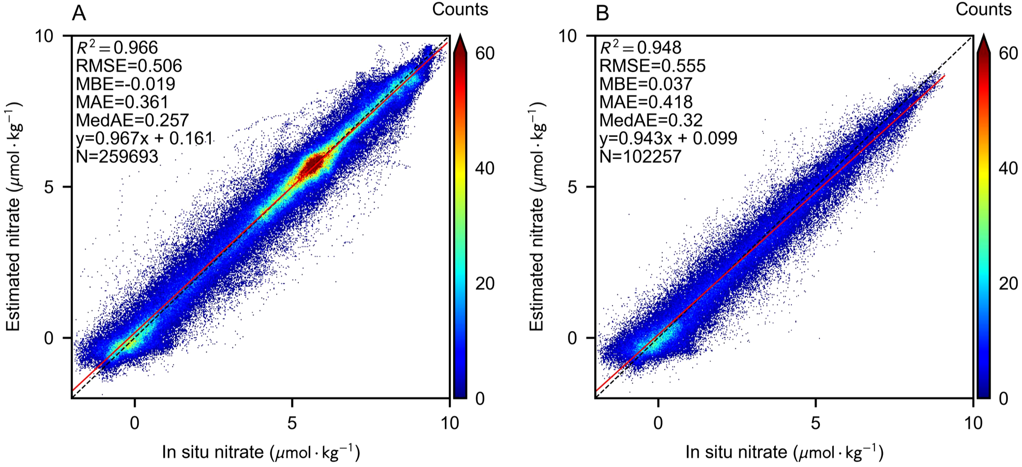
Scatter density plot of BNN estimation performance compared with in-situ nitrate measurements. The red line represents the data fit, while the black dashed line indicates the 1:1 reference line. (A) BNN performance with FS1 features. (B) BNN performance with FS2 features.
Figure 3 shows the comparison of vertical and monthly averaged patterns between BNN-modeled values and in-situ measurements, along with their associated uncertainties. The distribution patterns of the estimated values closely match those of the in situ values, demonstrating the vertical and temporal stability of the estimation performance. In contrast, predictions using FS2 exhibit higher uncertainty. This is because when only depth, temperature, and salinity are used as features in FS1, the model’s expressive power is limited, and the probability distribution in the BNN tends to stabilize. However, when additional features from Groups 2 and 3 are incorporated, the BNN gains stronger representational capacity, incorporating more patterns and variability, yet this inevitably elevates the variance in its estimated labels.
Figure 3
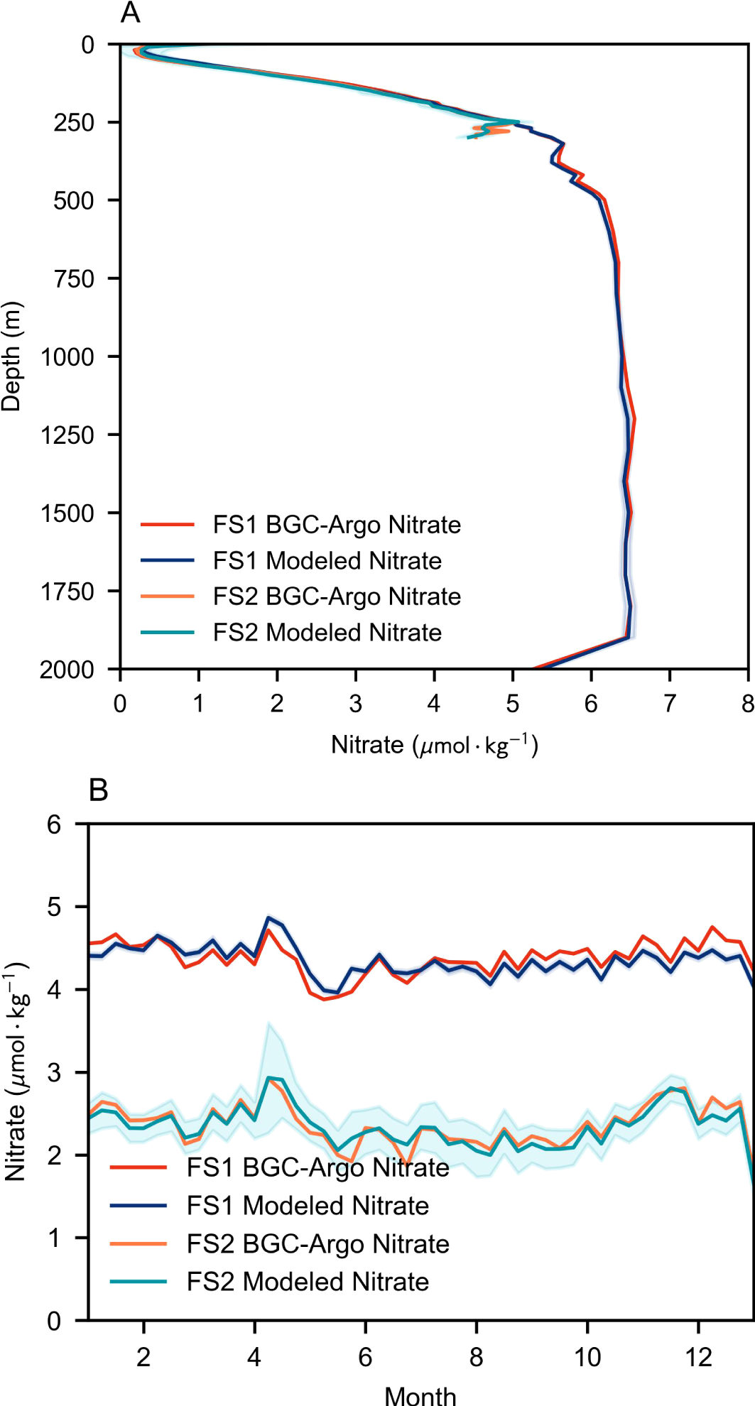
Comparison of BNN-modeled nitrate distribution profiles with BGC-Argo measurements in the test set. The shaded area represents the uncertainty range, magnified by a factor of 10 for clarity, corresponding to the case with k=10 in Equation 7. (A) Depth profile of nitrate distribution. (B) Monthly average profile of nitrate distribution.
Figures 4 and 5 show the horizontal distribution of the BNN test set errors and the uncertainty of the estimated augmented labels, further evaluating the impact of the observational range. Under both feature combinations, the model’s accuracy and uncertainty remain generally consistent in the horizontal direction. Higher errors and uncertainties tend to appear at the edges of the estimation range, where the input features accepted by the BNN deviate from the distribution observed during training, leading to greater divergence in its probability weight distribution. In this scenario, the weighted loss in Equation 7 effectively mitigates the adverse impact of low-quality labels on model training by leveraging uncertainty. For the observational range, estimated labels using only FS1 features cover nearly the entire study area, which is crucial for providing a broader view of the distribution patterns. At the same time, the estimation using FS2 features significantly supplements the label range. In this range, the augmented estimated labels provide additional biogeochemical knowledge of the upper ocean, enabling the reconstruction model to potentially fit a more generalized distribution pattern and oceanic process knowledge.
Figure 4
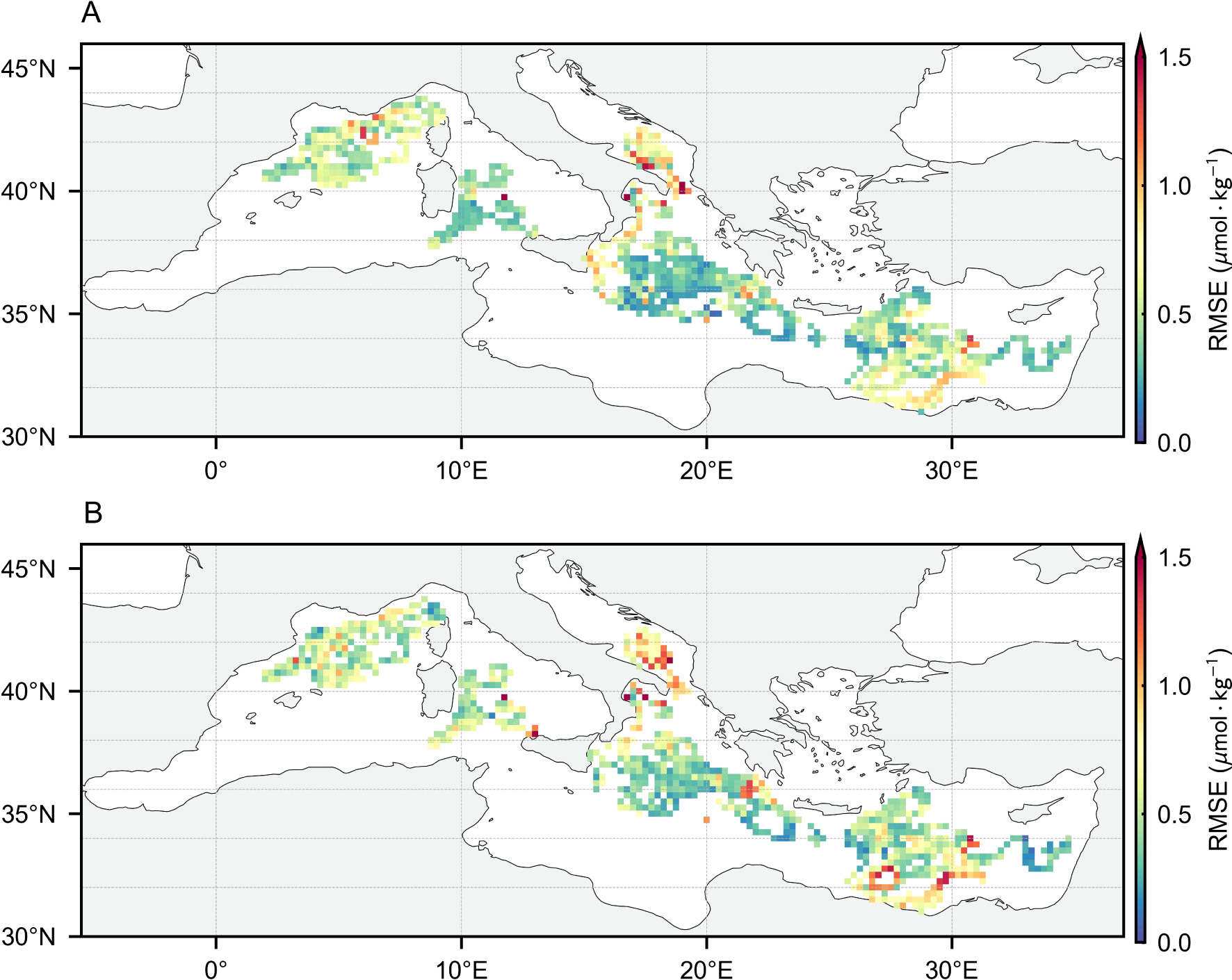
The horizontal distribution of BNN test set RMSE using synchronous observations with FS1 (A) and FS2 (B).
Figure 5
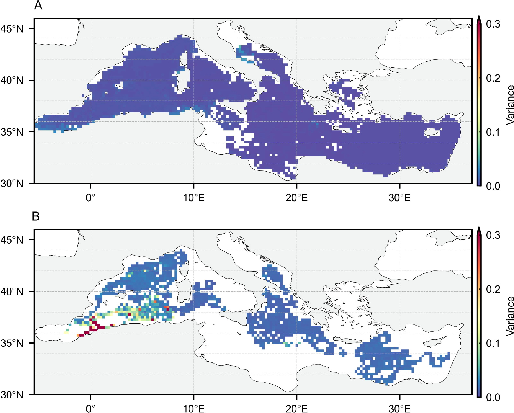
The horizontal distribution of BNN estimated label uncertainty using asynchronous observations with FS1 (A) and FS2 (B).
For nitrate 3D reconstruction label augmentation, the requirement is stable accuracy and appropriate uncertainty. Stable accuracy ensures that the estimated labels contribute beneficially to the training of the reconstruction model, while appropriate uncertainty helps balance the weight of in-situ and estimated labels in spatial reconstruction. Based on the above analysis, the BNN model’s augmented labels effectively meet both of these requirements.
3.3 Cruise independent validation
In this section, we present the model training and evaluation process, leveraging BGC-Argo data and augmented estimated labels for training, while employing the GLODAPv2 cruise measurement dataset for validation. Figure 6 illustrates the accuracy assessment of the test set, where each scatter point corresponds to a unique longitude-latitude-depth grid. The evaluation dataset comprises observational data collected during lateral cruises in the southern-central Mediterranean in 2011 and 2013. These cruises occurred at spatiotemporal locations that are significantly distinct from the BGC-Argo dataset, thereby posing a complex estimation challenge.
Figure 6
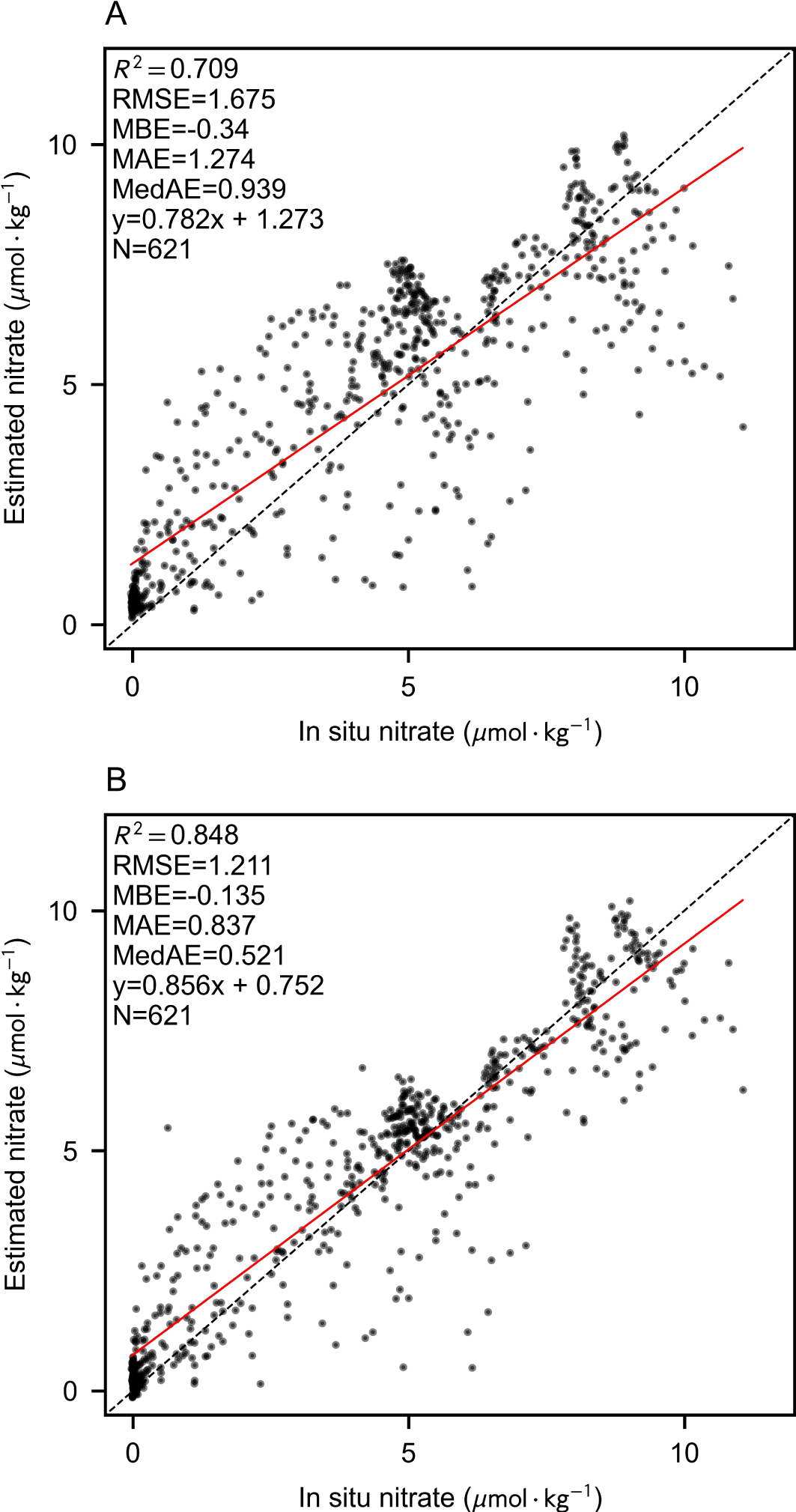
3D estimation performance verified by comparing cruise measurements using only BGC-Argo labels (A) or both augmented labels (B).
Following label augmentation, the Unet model demonstrated a substantial reduction in predictive uncertainty, elevating the R2 value from 0.709 to 0.848 and concurrently decreasing multiple error metrics. Notably, the BGC-Argo dataset does not encompass the region east of the Strait of Gibraltar, where nitrate concentrations within the Mediterranean exhibit elevated levels. Consequently, models trained exclusively on in-situ labels exhibited a systematic underestimation of nitrate concentrations in high-value regions. The integration of augmented labels effectively mitigated this bias, leading to improved predictive performance in these areas.
3.4 BGC-Argo performance validation
This section presents a rigorous evaluation of the model’s performance using BGC-Argo datasets, wherein training is conducted on post-2016 data with in situ and augmented estimated labels, while testing utilizes observational labels from BGC-Argo measurements between 2012 and 2015, strictly excluding estimated labels. Figure 7 provides a comparative assessment of model efficacy on the pre-2015 test set, with each scatter point corresponding to a distinct 3D grid unit. The integration of augmented labels and an optimized loss function yielded substantial improvements in predictive accuracy, as evidenced by an increased R2 value and a reduction in multiple error metrics. The incorporation of augmented labels facilitates the model’s ability to discern intricate relationships between upper-ocean variables and nitrate concentration, thereby enhancing its robustness and generalization capacity.
Figure 7
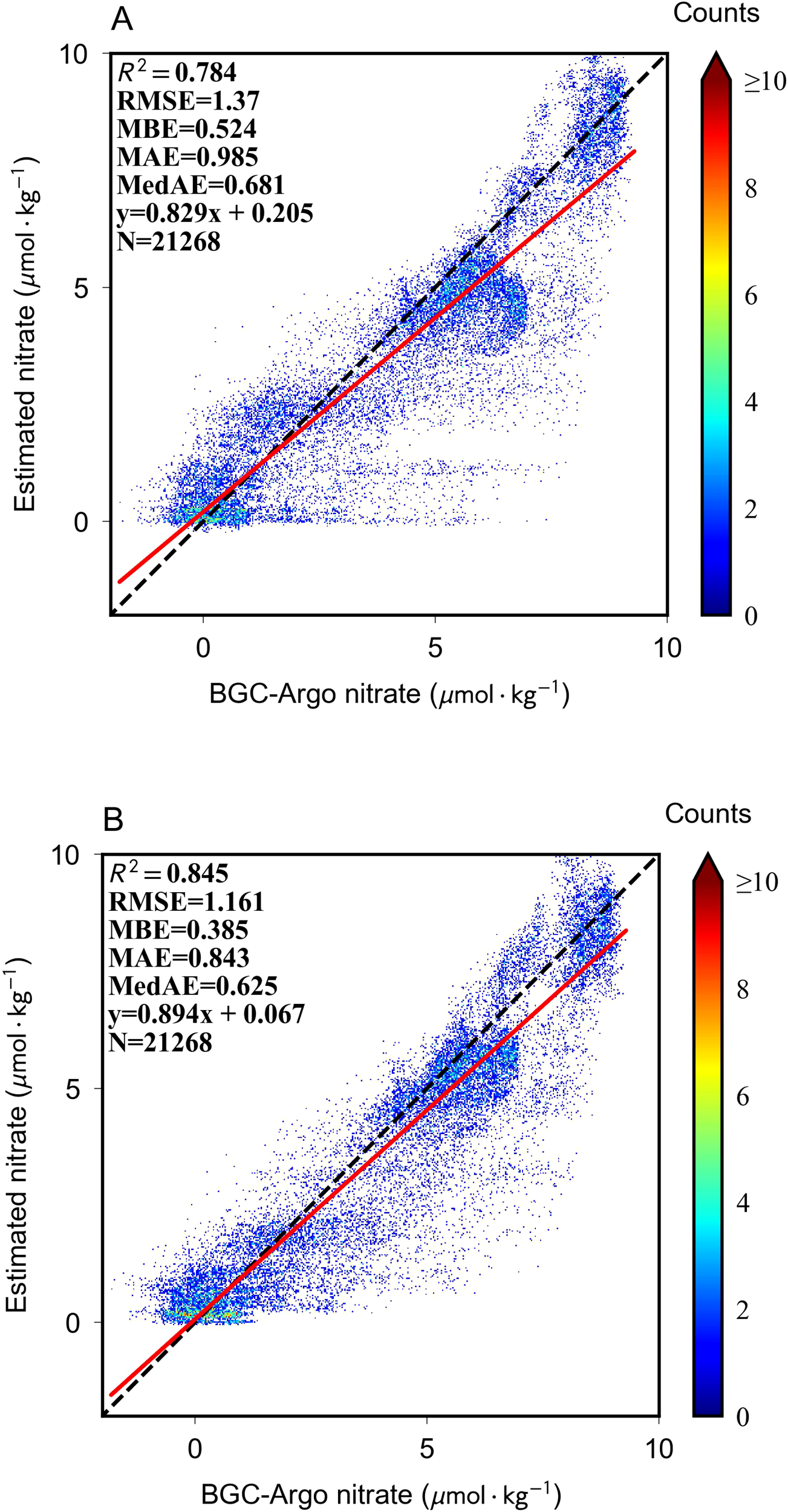
3D estimation performance verified by comparing BGC-Argo measurements using only BGCArgo labels (A) or both augmented labels (B).
As depicted in Figure 7A, the model demonstrates a pronounced tendency to underestimate nitrate concentrations in specific low-concentration samples, with extreme cases displaying near-zero anomalous estimates. This systematic bias stems primarily from the model’s reliance on sparse BGC-Argo observational labels during training, resulting in suboptimal generalization when applied to spatiotemporally diverse test conditions. The introduction of augmented labels mitigates this limitation, significantly enhancing both the model’s predictive performance and its capacity to capture meaningful estimation patterns. In cases of near-zero nitrate concentration, the predicted values exhibit a more uniform distribution, effectively reducing the prevalence of anomalous outliers. Furthermore, the model’s predictions for moderate and high-nitrate concentration clusters align more closely with the 1:1 reference line, reinforcing the validity of its estimation accuracy and generalization potential. These findings underscore the critical role of exposure to diverse upper-ocean patterns during training in fostering a more comprehensive feature-learning mechanism, ultimately improving the model’s adaptability to previously unobserved data.
3.5 Impact of augmented estimated labels on model performance
We conducted two types of 3D estimation performance tests, each focusing on different aspects of the model’s generalization ability. The validation test using BGC-Argo data primarily assessed the model’s temporal generalization capability. BGC-Argo observation sites are relatively concentrated and predominantly located in the northeastern Mediterranean (Figure 4). When BGC-Argo provided test labels from before 2015, there were usually corresponding observations available from nearby locations after 2016. In contrast, the independent cruise validation simultaneously evaluated both spatial and temporal generalization. The cruises were conducted in 2011 and 2013, preceding the large-scale observations of BGC-Argo. Sampling sites spanned the Mediterranean, with some located in the southwestern region, an area not effectively covered by BGC-Argo. This region is connected to the Atlantic Ocean via the Strait of Gibraltar and exhibits high nitrate levels. Consequently, the GLODAP samples exhibit significant spatiotemporal differences from BGC-Argo data, posing a comprehensive test of the model’s ability to generalize across both time and space.
Comparing the two validation approaches, results indicate that the augmented label method generally improved both spatial and temporal generalization of the model. More specifically, the model demonstrated a more pronounced gain in spatial generalization capability from the augmented labels, aligning with the conceptual role of label augmentation. Through the inclusion of augmented labels, the model acquired knowledge beyond the scope of BGC-Argo, enhancing its ability to fit the relationship between surface ocean conditions and nitrate concentration. This gain is particularly crucial for improving spatial generalization.
To further evaluate the impact of different augmented labels on model improvement, Figure 8 presents the vertical RMSE distribution and optimal proxy under various label combinations. The results indicate that the introduction of all augmented labels significantly reduces model estimation errors overall. The model trained with both FS1 and FS2 labels achieves the highest overall accuracy and vertical stability. Two prominent error peaks appear in the upper ocean at 0 meters and approximately 100 meters, corresponding to the air-sea interface and the lower boundary of the oceanic mixed layer, respectively. These regions are characterized by complex environmental interactions, making it particularly challenging to model the relationship between oceanographic features and nitrate concentrations. Notably, the augmented labels lead to significant improvements in model performance within the upper ocean, effectively reducing error peaks and minimizing overall errors throughout this layer, while also positively impacting the mid-ocean region.
Figure 8
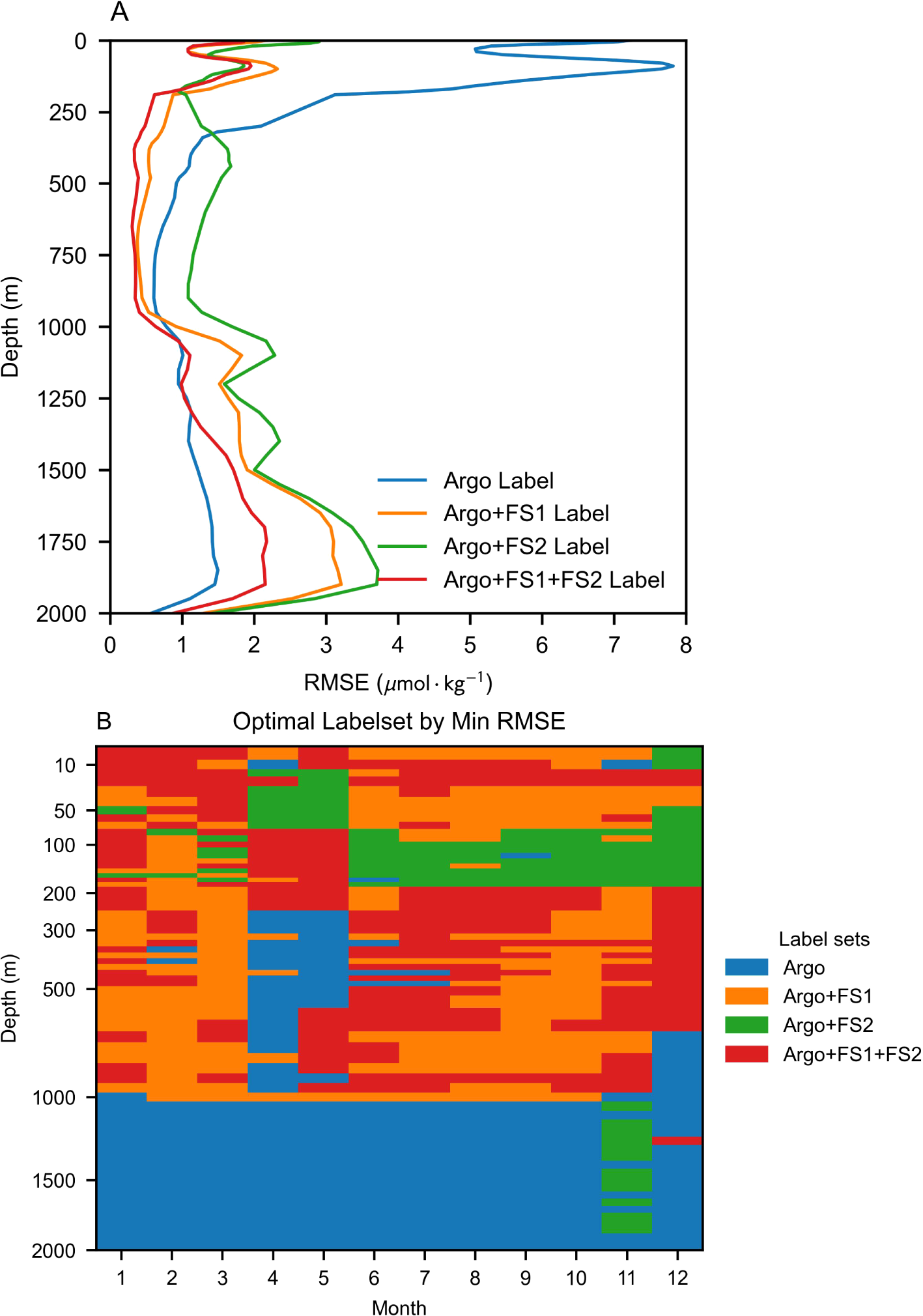
3D nitrate estimation performance of the model under different label combinations. (A) Trend profiles depicting the variation of model performance with depth. (B) Distribution of label sets achieving optimal RMSE performance across different depth and temporal cases.
Regarding the optimal feature combinations for different depths and seasonal cases (Figure 8B), FS1 label augmentation emerges as the most influential. While models augmented with both FS1 and FS2 labels dominate as optimal proxies across most scenarios, models incorporating FS1 alone also achieve superior performance in a substantial number of cases. The roles of the two label sets differ: FS1 labels significantly expands the sample diversity, increasing the number of labels by more than 50 times (Table 1), whereas FS2 labels focuses on refining the fit for upper-ocean nitrate dynamics. Scenarios where FS2-only augmentation yields the best performance are primarily found within the 0-200m depth range, particularly during spring and the latter half of the year, aligning with the intended function of FS2 labels.
At depths exceeding 1000 m, the optimal configuration remains the exclusive use of BGC-Argo observational labels. This is because, given that BGC-Argo testing primarily evaluates the model’s temporal extrapolation ability, deep-sea nitrate concentrations in this range remain nearly invariant over time. The introduction of estimated labels inevitably disturbs the inherent spatial regularity encoded within BGC-Argo labels, weakening the model’s ability to fit deep-sea nitrate concentrations at specific spatial coordinates. Nevertheless, the RMSE increase at depths beyond 1000 m remains marginal when both FS1 and FS2 labels are incorporated (Figure 8B), indicating that the augmented label interference propagates uniformly across all scenarios within this depth range. Compared to the overall performance improvement, this minor trade-off is acceptable, as the upper ocean is the more dynamic and critical region where enhancements in model performance yield the most significant benefits.
From another perspective, fitting deep-sea nitrate concentrations too closely to observations poses a risk of overfitting in global 3D oceanic nitrate estimation. Deep-sea nitrate levels are more influenced by geographic location than by temporal variations, and the limited spatial coverage of BGC-Argo observations constitutes a fundamental constraint. The deep-sea nitrate measurements provided by BGC-Argo may inadvertently restrict model generalization in unobserved oceanic regions. In contrast, the augmented labels contribute positively to high-concentration deep-sea regions in independent cruise validation (Figure 6B), underscoring their utility in enhancing model generalization beyond BGC-Argo’s observational domain.
4 Conclusion
This paper proposes a novel method for 3D nitrate estimation in marine environments using deep learning techniques, particularly through the fusion of underwater signals and label augmentation. A key challenge in marine nitrate modeling lies in the scarcity and spatiotemporal limitations of in situ data. To address this issue, the study employs BNN to enhance nitrate labels, with a focus on uncertainty quantification. By integrating both real and augmented labels into a U-Net-based deep learning framework, the study successfully improves the model’s ability to estimate nitrate concentrations in the Mediterranean. The uncertainty-weighted loss function further refines the model’s performance, enabling it to address both data gaps and the inherent uncertainties of augmented labels.
The results demonstrate a significant enhancement in the model’s spatial and temporal generalization, especially in regions with limited sampling. Validation using BGC-Argo and GLODAPv2 shipboard data confirms that this method can more accurately and comprehensively reconstruct the 3D distribution of nitrates. These findings underscore the value of integrating sub-surface indicators with Bayesian uncertainty-aware label augmentation to improve the precision and robustness of marine biogeochemical models.
One of the major contributions of this work is its potential for broader application in environmental monitoring and climate-related research. By filling data gaps in poorly observed areas, this method offers a scalable solution for large-scale, continuous monitoring of marine ecosystems. It can be extended to other marine regions, providing deeper insights into global nutrient distribution and aiding in more informed predictions of marine productivity, carbon sequestration, and oceanic processes under changing climate conditions. Future work will focus on further refining the model, incorporating more environmental variables, or exploring hybrid approaches that combine numerical models with deep learning frameworks. Additionally, expanding the research to more diverse marine regions and improving the temporal resolution of data will present further opportunities to enhance the model’s predictive capabilities.
In summary, this study provides a robust framework for 3D nitrate estimation, marking a significant step forward in marine biogeochemical modeling. The integration of deep learning with label augmentation and uncertainty quantification presents a promising approach to overcoming the challenges posed by data scarcity, ultimately contributing to more accurate and comprehensive assessments of marine ecosystems.
Statements
Data availability statement
The original contributions presented in the study are included in the article/supplementary material. Further inquiries can be directed to the corresponding author.
Author contributions
XY: Data curation, Methodology, Validation, Visualization, Writing – original draft. GF: Conceptualization, Funding acquisition, Supervision, Writing – review & editing. JL: Conceptualization, Supervision, Writing – review & editing.
Funding
The author(s) declare that financial support was received for the research and/or publication of this article. The study was supported through the National Natural Science Foundation of China (42176010).
Acknowledgments
The authors thank the International Argo Program, European Space Agency, European Centre for MediumRange Weather Forecasts (ECMWF), Copernicus Climate Change Service, and GLODAPv2 for data, which are freely accessible for public. The BGC-Argo data were collected and made freely available by the International Argo Program and the national programs that contribute to it (https://argo.ucsd.edu, https://www.ocean-ops.org). The Argo Program is part of the Global Ocean Observing System. Biogeochemical data are from the European Copernicus Marine Environmental Monitoring Service (CMEMS, https://marine.copernicus.eu). The GlobColour data used in this study has been developed, validated, and distributed by ACRI-ST, France (http://globcolour.info). The ERA5 data are from the Copernicus Climate Change Service (https://cds.climate.copernicus.eu).
Conflict of interest
The authors declare that the research was conducted in the absence of any commercial or financial relationships that could be construed as a potential conflict of interest.
Generative AI statement
The author(s) declare that no Generative AI was used in the creation of this manuscript.
Publisher’s note
All claims expressed in this article are solely those of the authors and do not necessarily represent those of their affiliated organizations, or those of the publisher, the editors and the reviewers. Any product that may be evaluated in this article, or claim that may be made by its manufacturer, is not guaranteed or endorsed by the publisher.
References
1
Baretta J. W. Ebenhöh W. Ruardij P. (1995). The European regional seas ecosystem model, a complex marine ecosystem model. Neth. J. Sea Res.33, 233–246. doi: 10.1016/0077-7579(95)90047-0
2
Bittig H. C. Steinhoff T. Claustre H. Fiedler B. Williams N. L. Sauzède R. et al . (2018). An alternative to static climatologies: Robust estimation of open ocean CO2 variables and nutrient concentrations from T, S, and O2 data using Bayesian neural networks. Front. Mar. Sci.5. doi: 10.3389/fmars.2018.00328
3
Blundell C. Cornebise J. Kavukcuoglu K. Wierstra D. (2015). “Weight uncertainty in neural network,” in Proceedings of the 32nd international conference on machine learning (PMLR), 1613–1622.
4
Bristow L. A. Mohr W. Ahmerkamp S. Kuypers M. M. (2017). Nutrients that limit growth in the ocean. Curr. Biol.27, R474–R478. doi: 10.1016/j.cub.2017.03.030
5
Bruggeman J. Bolding K. (2014). A general framework for aquatic biogeochemical models. Environ. Modell. Software61, 249–265. doi: 10.1016/j.envsoft.2014.04.002
6
Buongiorno Nardelli B. (2020). A deep learning network to retrieve ocean hydrographic profiles from combined satellite and in situ measurements. Remote Sens.12, 3151.
7
Chang N.-B. Xuan Z. Yang Y. J. (2013). Exploring spatiotemporal patterns of phosphorus concentrations in a coastal bay with MODIS images and machine learning models. Remote Sens. Environ.134, 100–110. doi: 10.1016/j.rse.2013.03.002
8
Chen S. Meng Y. Lin S. Yu Y. Xi J. (2023). Estimation of sea surface nitrate from space: Current status and future potential. Sci. Total Environ.899, 165690. doi: 10.1016/j.scitotenv.2023.165690
9
Cheng Z. Fan G. Zhou J. Gan M. Chen C. L. P. (2025). FDCE-net: Underwater image enhancement with embedding frequency and dual color encoderenglish. IEEE Trans. Circuits Syst. Video Technol.35, 1728–1744. doi: 10.1109/TCSVT.2024.3482548
10
Claustre H. Johnson K. S. Takeshita Y. (2020). Observing the global ocean with biogeochemicalArgo. Annu. Rev. Mar. Sci.12, 23–48. doi: 10.1146/annurev-marine-010419-010956
11
Eppley R. W. Peterson B. J. (1979). Particulate organic matter flux and planktonic new production in the deep ocean. Nature282, 677–680. doi: 10.1038/282677a0
12
Feng Y. Ma L. Meng X. Zhou F. Liu R. Su Z. (2024). Advancing real-world image dehazing: Perspective, modules, and trainingenglish. IEEE Trans. Pattern Anal. Mach. Intell.46, 9303–9320. doi: 10.1109/TPAMI.2024.3416731
13
Fourrier M. Coppola L. Claustre H. D’Ortenzio F. Gattuso J. P. (2020). A regional neural network approach to estimate water-column nutrient concentrations and carbonate system variables in the mediterranean sea: CANYON-MED. Front. Mar. Sci.7. doi: 10.3389/fmars.2020.00620
14
Friedlingstein P. O’sullivan M. Jones M. W. Andrew R. M. Hauck J. Olsen A. et al . (2020). Global carbon budget 2020. Earth Syst. Sci. Data12, 3269–3340. doi: 10.5194/essd-12-3269-2020
15
Gao H. Huang B. Chen G. Xia L. Radenkovic M. (2024). Deep learning solver unites SDGSAT-1 observations and navier–stokes theory for oceanic vortex streetsenglish. Remote Sens. Environ.315, 114425. doi: 10.1016/j.rse.2024.114425
16
Goes J. I. Saino T. Oaku H. Jiang D. L. (1999). A method for estimating sea surface nitrate concentrations from remotely sensed SST and chlorophyll aa case study for the north Pacific Ocean using OCTS/ADEOS data. IEEE Trans. Geosci. Remote Sens.37, 1633–1644. doi: 10.1109/36.763279
17
Gregg W. W. Conkright M. E. Ginoux P. O’Reilly J. E. Casey N. W. (2003). Ocean primary production and climate: Global decadal changes. Geophys. Res. Lett.30, 1089. doi: 10.1029/2003GL016889
18
Hersbach H. Bell B. Berrisford P. Hirahara S. Horányi A. Muñoz-Sabater J. et al . (2020). The ERA5 global reanalysis. Q. J. R. Meteorolog. Soc146, 1999–2049. doi: 10.1002/qj.3803
19
Holt J. Butenschön M. Wakelin S. L. Artioli Y. Allen J. I. (2012). Oceanic controls on the primary production of the northwest European continental shelf: Model experiments under recent past conditions and a potential future scenario. Biogeosciences9, 97–117. doi: 10.5194/bg-9-97-2012
20
Hu Q. Chen X. Bai Y. He X. Li T. Pan D. (2023). Reconstruction of 3-D ocean chlorophyll a structure in the northern Indian ocean using satellite and BGC-argo data. IEEE Trans. Geosci. Remote Sens.61, 1–13. doi: 10.1109/TGRS.2022.3233385
21
Johnson K. Maurer T. Plant J. Bittig H. Schallenberg C. Schmechtig C. (2021). BGC-Argo quality control manual for nitrate concentration. doi: 10.13155/84370
22
Johnson K. S. Plant J. N. Coletti L. J. Jannasch H. W. Sakamoto C. M. Riser S. C. et al . (2017). Biogeochemical sensor performance in the SOCCOM profiling float array. J. Geophys. Res.: Oceans122, 6416–6436. doi: 10.1002/2017JC012838
23
Johnson K. S. Plant J. N. Sakamoto C. Maurer T. L. Pasqueron De Fommervault O. Serra R. et al . (2024). Processing BGC-Argo nitrate concentration at the DAC Level. doi: 10.13155/46121
24
Kay S. Butenschön M. (2018). Projections of change in key ecosystem indicators for planning and management of marine protected areas: An example study for European seas. Estuar. Coast. Shelf Sci.201, 172–184. doi: 10.1016/j.ecss.2016.03.003
25
Lauvset S. K. Lange N. Tanhua T. Bittig H. C. Olsen A. Kozyr A. et al . (2021). An updated version of the global interior ocean biogeochemical data product, GLODAPv2.2021. Earth Syst. Sci. Data13, 5565–5589. doi: 10.5194/essd-13-5565-2021
26
Lauvset S. K. Lange N. Tanhua T. Bittig H. C. Olsen A. Kozyr A. et al . (2022). GLODAPv2.2022: The latest version of the global interior ocean biogeochemical data product. Earth Syst. Sci. Data14, 5543–5572. doi: 10.5194/essd-14-5543-2022
27
Lavender S. Antoine D. Maritorena S. Morel A. Barrot G. Demaria J. et al . (2009). “GlobColour—The European service for ocean colour,” in Proceedings of the 2009 IEEE international geoscience & Remote sensing symposium (“IEEE Geoscience and Remote Sensing Society: Cape Town, South Africa), 12–17.
28
Lavigne H. D’ortenzio F. Ribera D’Alcalà M. Claustre H. Sauzède R. Gacic M. (2015). On the vertical distribution of the chlorophyll a concentration in the Mediterranean Sea: A basin-scale and seasonal approach. Biogeosciences12, 5021–5039. doi: 10.5194/bgd-12-4139-2015
29
Mignot A. D’Ortenzio F. Taillandier V. Cossarini G. Salon S. (2019). Quantifying observational errors in biogeochemical-argo oxygen, nitrate, and chlorophyll a concentrations. Geophys. Res. Lett.46, 4330–4337. doi: 10.1029/2018GL080541
30
Nittis K. Tziavos C. Bozzano R. Cardin V. Thanos Y. Petihakis G. et al . (2007). The M3A multisensor buoy network of the Mediterranean Sea. Ocean Sci.3, 229–243. doi: 10.5194/os-3-229-2007
31
Olsen A. Lange N. Key R. M. Tanhua T. Bittig H. C. Kozyr A. et al . (2020). An updated version of the global interior ocean biogeochemical data product, GLODAPv2.2020. Earth Syst. Sci. Data12, 3653–3678. doi: 10.5194/essd-12-3653-2020
32
Pan X. Wong G. T. Ho T.-Y. Tai J.-H. Liu H. Liu J. et al . (2018). Remote sensing of surface [nitrite+ nitrate] in river-influenced shelf-seas: The northern South China Sea Shelf-sea. Remote Sens. Environ.210, 1–11. doi: 10.1016/j.rse.2018.03.012
33
Qi J. Liu C. Chi J. Li D. Gao L. Yin B. (2022). An ensemble-based machine learning model for estimation of subsurface thermal structure in the south China sea. Remote Sens.14, 3207. doi: 10.3390/rs14133207
34
Rafter P. A. Sigman D. M. Mackey K. R. (2017). Recycled iron fuels new production in the eastern equatorial Pacific Ocean. Nat. Commun.8, 1–10. doi: 10.1038/s41467-017-01219-7
35
Ronneberger O. Fischer P. Brox T. (2015). “U-net: Convolutional networks for biomedical image segmentation,” in Medical image computing and computer-assisted intervention – MICCAI 2015. Eds. NavabN.HorneggerJ.WellsW. M.FrangiA. F. (Springer International Publishing, Cham), 234–241. doi: 10.1007/978-3-319-24574-428
36
Sathyendranath S. Platt T. Horne E. P. Harrison W. G. Ulloa O. Outerbridge R. et al . (1991). Estimation of new production in the ocean by compound remote sensing. Nature353, 129–133. doi: 10.1038/353129a0
37
Sauzède R. Bittig H. C. Claustre H. Pasqueron de Fommervault O. Gattuso J.-P. Legendre L. et al . (2017). Estimates of water-column nutrient concentrations and carbonate system parameters in the global ocean: A novel approach based on neural networks. Front. Mar. Sci.4. doi: 10.3389/fmars.2017.00128
38
Smith P. A. H. Sørensen K. A. Buongiorno Nardelli B. Chauhan A. Christensen A. St. John M. et al . (2023). Reconstruction of subsurface ocean state variables using Convolutional Neural Networks with combined satellite and in situ data. Front. Mar. Sci.10. doi: 10.3389/fmars.2023.1218514
39
Su H. Zhang T. Lin M. Lu W. Yan X.-H. (2021). Predicting subsurface thermohaline structure from remote sensing data based on long short-term memory neural networks. Remote Sens. Environ.260, 112465. doi: 10.1016/j.rse.2021.112465
40
Tian T. Cheng L. Wang G. Abraham J. Wei W. Ren S. et al . (2022). Reconstructing ocean subsurface salinity at high resolution using a machine learning approach. Earth Syst. Sci. Data14, 5037–5060. doi: 10.5194/essd-14-5037-2022
41
Wang L. Xu Z. Gong X. Zhang P. Hao Z. You J. et al . (2023). Estimation of nitrate concentration and its distribution in the northwestern Pacific Ocean by a deep neural network model. Deep Sea Res. Part I195, 104005. doi: 10.1016/j.dsr.2023.104005
42
Yang G. G. Wang Q. Feng J. He L. Li R. Lu W. et al . (2024). Can three-dimensional nitrate structure be reconstructed from surface information with artificial intelligence? — a proof-of-concept study. Sci. Total Environ.924, 171365. doi: 10.1016/j.scitotenv.2024.171365
43
Yang S. Zhang J. Wang J. Zhang S. Bai Y. Shi S. et al . (2022). Spatiotemporal variations of water productivity for cropland and driving factors over China during 2001–2015english. Agric. Water Manage.262, 107328. doi: 10.1016/j.agwat.2021.107328
44
Yu X. Chen S. Chai F. (2022). Remote estimation of sea surface nitrate in the california current system from satellite ocean color measurements. IEEE Trans. Geosci. Remote Sens.60, 1–17. doi: 10.1109/TGRS.2021.3095099
45
Yuan Q. Shen H. Li T. Li Z. Li S. Jiang Y. et al . (2020). Deep learning in environmental remote sensing: Achievements and challenges. Remote Sens. Environ.241, 111716. doi: 10.1016/j.rse.2020.111716
46
Zhang D. Lu L. Li X. Zhang J. Zhang S. Yang S. (2024). Spatial downscaling of ESA CCI soil moisture data based on deep learning with an attention mechanismenglish. Remote Sens.16, 1394. doi: 10.3390/rs16081394
47
Zhou L. Zhang R.-H. (2023). A self-attention–based neural network for three-dimensional multivariate modeling and its skillful ENSO predictions. Sci. Adv.9, eadf2827. doi: 10.1126/sciadv.adf2827
Summary
Keywords
three-dimensional nitrate estimation, BGC-Argo, Mediterranean Sea, Bayesian neural network, label augmentation, U-net
Citation
Yu X, Fan G and Li J (2025) Deep learning-driven 3D marine nitrate estimation: uncertainty mitigation through underwater signal exploitation and label augmentation. Front. Mar. Sci. 12:1576558. doi: 10.3389/fmars.2025.1576558
Received
14 February 2025
Accepted
17 March 2025
Published
08 April 2025
Volume
12 - 2025
Edited by
Yakun Ju, University of Leicester, United Kingdom
Reviewed by
Dehuan Zhang, Dalian Maritime University, China
Linghui Xia, Ocean University of China, China
Updates
Copyright
© 2025 Yu, Fan and Li.
This is an open-access article distributed under the terms of the Creative Commons Attribution License (CC BY). The use, distribution or reproduction in other forums is permitted, provided the original author(s) and the copyright owner(s) are credited and that the original publication in this journal is cited, in accordance with accepted academic practice. No use, distribution or reproduction is permitted which does not comply with these terms.
*Correspondence: Guodong Fan, fgd96@outlook.com
Disclaimer
All claims expressed in this article are solely those of the authors and do not necessarily represent those of their affiliated organizations, or those of the publisher, the editors and the reviewers. Any product that may be evaluated in this article or claim that may be made by its manufacturer is not guaranteed or endorsed by the publisher.