A novel framework for identifying fishing grounds from AIS data containing vessels of unknown types

To address the issue of precisely identifying fishing grounds in vast sea areas, this study proposes a framework that includes a fishing behavior detection model and a fishing ground identification model, considering vessels of unknown types. The absence of information regarding unknown vessels can result in incomplete identification of fishing grounds, which in turn leads to regulatory oversight, and these unidentified fishing areas might be hotspots for illegal fishing activities. Identifying these missing fishing grounds is crucial for enhancing regulatory efforts and for vessels go through these areas to plan their routes more effectively in advance. This helps in finding illegal fishing and optimizes the operational efficiency of fishing vessels. Firstly, the Speed-Direction-Based Stops and Moves of Trajectories (SDB-SMOT) algorithm is proposed. Based on this algorithm, a fishing behavior detection model is developed to identify fishing activity trajectories from AIS data that encompasses vessels of unknown types. Subsequently, an algorithm that integrates the Data Field and OPTICS (DF-OPTICS) algorithm is proposed, and a model for identifying fishing grounds is constructed based on the DF-OPTICS algorithm. The efficiency and effectiveness of this framework are validated by identifying fishing grounds from AIS data that contains both fishing vessels and vessels of unknown types in the South China Sea. The Davies-Bouldin Index of DF-OPTICS algorithm reached 0.267, 0.224, 0.203, the Silhouette Coefficient Index reached 0.560, 0.598, 0.633 and the Calinski-Harabasz Index reached 2213939, 3296101, 4320688 under three sets of hyperparameters. This framework not only bridges the gap in identifying fishing grounds from AIS data containing vessels of unknown types but also improves the efficiency of the fishing ground identification process.

1 Introduction

Amidst the diminishing primary economic fishery resources in oceans worldwide, there is an increasing focus on the conservation and sustainable development and utilization of marine fishery resources. Fishing grounds are areas where fishery resources are concentrated. A large number of fishing vessels gather on these fishing grounds for fishing operations, activities, and navigation. The operational zones of these fishing vessels frequently overlap and intersect with the shipping routes of merchant vessels, thereby increasing the risk of collisions between merchant and fishing vessels. A comprehensive understanding of these fishing grounds is crucial as it can help the scientific management of marine fishery resources, guide the establishment of fishing industry regulations, and aid in planning merchant shipping routes and maritime traffic management (Hutniczak et al., 2024).

However, a certain number of vessels of unknown types exist in the AIS data due to illegal tampering, unfamiliar operations by seafarers, AIS equipment failure, failure of message transmission (Jeon and Han, 2022), etc. Among these unknown vessels, a certain proportion of them are fishing vessels. We put forward this point of view first of all on the basis of fact that the phenomenon of tampering and concealment of AIS data by fishing vessels is more common than other ship types, and the fishermen are far less professional in operating AIS than crews (Wu et al., 2024). AIS data with vessels of unknown types contains a lot of information about the fishing vessel and is essential for extracting the area where the fishing vessels operate.

Currently, research on the identification of fishing vessel activity areas mainly relies on four types of data: fish catch data (Fitrianah et al., 2016; Owiredu and Kim, 2021), nightly satellite data (Li et al., 2022), vessel monitoring system (VMS) data (Shi et al., 2024a), and Automatic Identification System (AIS) data (Zeng et al., 2024). Fish catch data, which can directly reflect the spatial and temporal activities of fishing vessels in a specific region, is typically reported by fishermen (Perez et al., 2024). However, this fish catch data can be compromised by its inherent imprecision, such as statistical errors or incomplete reports. Nightly satellite data collected through remote sensing of lights by an imaging sensor mounted on the satellite (Li et al., 2021) can describe the patterns and characteristics of fishing vessels’ activities at night. However, nightly satellite data is limited in monitoring fishing vessels at night, and the process of identifying fishing vessel tracks from satellite imagery can be easily impacted by clouds, moon phases, and lunar glare (Li et al., 2022). With the advancement of maritime surveillance technology, AIS and VMS have gradually become essential tools for studying the trajectory of vessels. VMS data is subject to strict access controls, with the flag state being the sole entity authorized to protect and receive such information. This creates significant difficulties in collecting data on fishing vessels from different countries (Yan et al., 2022). The high installation costs are also challenges to promoting their use among offshore fishing vessels. In contrast to VMS data, AIS data has gradually become the primary data source for research on the trajectory of vessels due to the low costs and ease of accessibility (Huang et al., 2023; Chen et al., 2024).

Before analyzing fishing areas for fishing vessels, it is essential to identify their behavior patterns. The most common approach for this is the statistics-based model, which typically focuses on the speed or course of fishing vessels (Natale et al., 2015; Chen et al., 2022; Yan et al., 2022). However, relying solely on the analysis of either speed or course can provide only a partial view of their behavior. In recent years, scholars have used machine learning and deep learning techniques to identify fishing vessel behaviors (Wu et al., 2022; Yang et al., 2024). However, the process remains complex and is often confined to a single category of vessels. The most commonly used methods in studying fishing vessel activities from trajectory data center around estimating fishing effort, calculating vessel emissions, and directly analyzing AIS data (Coello et al., 2015; Sun et al., 2023; Cappa et al., 2024). These techniques mainly generate heat maps of fishing vessel activities but fall short of providing accurate information on fishing vessel activity areas.

This study proposes a framework to identify fishing grounds. Firstly, the Speed-Direction-Based Stops and Moves of Trajectories (SDB-SMOT) algorithm is proposed, which forms the foundation for a fishing behavior detection model. Subsequently, the fishing behavior model is applied to AIS data with vessels of unknown types. Secondly, the study further improves the Ordering Points To Identify the Clustering Structure (OPTICS) algorithm by incorporating knowledge from the Data Field (DF) theory. A fishing grounds identification model is developed based on the improved algorithm, Ordering Points To Identify the Clustering Structure Considering Data Field (DF-OPTICS). The main contributions of this paper are as follows:

1. This study establishes a framework for identifying fishing grounds from AIS data containing both fishing vessels and vessels of unknown types.

2. This study proposes the SDB-SMOT algorithm. Based on the algorithm, the fishing behavior detection model is established, which can successfully identify fishing trajectories from AIS data containing vessels of unknown types.

3. An improved algorithm, DF-OPTICS, is proposed. Initially, it merges knowledge from the DF and OPTICS algorithms, addressing the challenge of selecting points with the same reachability distance. It performs better clustering than three existing algorithms, the traditional OPTICS algorithm, the DBSCAN algorithm, and the improved OPTICS algorithm, using automatic identification of clusters, particularly on large-scale trajectory datasets. Based on the DF-OPTICS algorithm, the fishing grounds identification model is established.

4. The framework for fishing ground identification has been applied to the South China Sea. It successfully reveals distinct quarterly variations in the spatial and temporal characteristics of fishing vessel activities in the South China Sea.

The remainder of this paper is organized as follows. Section 2 reviews the related studies of fishing behavior detection and fishing grounds identification. Section 3 introduces the principles of our method, including the SDB-SMOT algorithm, the principle of the DF-OPTICS algorithm, and the establishment of the fishing behavior detection model and fishing grounds identification model. Section 4 shows fishing grounds identification results and the cluster outcomes, followed by a comparative analysis. This analysis evaluates the performance of the DF-OPTICS algorithm against three other algorithms using three key clustering evaluation indexes: Silhouette Coefficient (SC) (Bagirov et al., 2023), Calinski-Harabasz Index (CHI) (Solorio-Fernández et al., 2016) and Davies-Bouldin Index (DBI) (Liu et al., 2011). The efficiency and effectiveness of this framework in identifying fishing grounds from vessels of unknown types are also demonstrated. The conclusions are discussed in Section 5.

2 Literature review

Recent approaches to identifying fishing grounds generally fall into behavior detection and fishing grounds identification. This section provides an overview of the current methods used for identifying fishing grounds. Moreover, it highlights the existing gaps in the literature related to this field.

2.1 Behavior detection

The methods of behavior detection mainly include statistical models and machine learning. In the study of statistical models, Natale et al. (2015) analyzed the speed profiles of offshore fishing vessels. They concluded that the bimodal curve of fishing vessel speed follows a Gaussian mixture distribution. This method has been adopted widely in the study of fishing vessel activities (James et al., 2018; Campos et al., 2023; Wan et al., 2024). Rocha et al. (2010) proposed a Direction-Based Spatio-Temporal Clustering Method based on the knowledge of stopping point identification, using the magnitude of course changes as the criterion for identifying fishing points. The above scholars have conducted research from two aspects: speed and course. Hu et al. (2016) ingeniously selected Conditional Random Fields (CRF) to identify precise characteristics of fishing vessel trajectories from AIS data, effectively identifying fishing activities. Peel and Good (2011) adopted the hidden Markov model approach to discover vessel activities, focusing on speed as the primary research object. Sun et al. (2023) conducted a thorough study of the spatial-temporal characteristics of fishing vessels, including their lengths, speeds, trajectories, trajectory densities, and the numbers of active vessels and their average fishing times, to accurately identify the states of fishing vessels. Using more characteristics to carry out fishing vessel behavior detection is not always beneficial, and redundant features can decrease the detection rate. Meanwhile, similar methodologies often result in fragments of fishing trajectories, failing to provide comprehensive and continuous trajectories of fishing activities.

Machine learning methods primarily involve selecting a model to be trained on a training dataset, making the steps of characteristic selection and model selection essential. Chuaysi and Kiattisin (2020) presented a new technique for analyzing local characteristics of time series data. They transformed the trajectory pattern into global characteristics for deep learning applications. However, due to technological constraints, relying solely on global characteristics is insufficient for investigating fishing activities on high seas, highlighting the need for more advanced methods to capture subtle patterns. Masroeri et al. (2021) proposed an integrated system with predictive capabilities to identify illegal fishing and transshipment occurrences. The predictive component was crafted utilizing Recurrent Neural Networks (RNNs), while the system integration leverages Artificial Neural Networks (ANNs). This approach aimed to enhance the efficiency and accuracy of oceanic fisheries monitoring, particularly in scenarios where data may be incomplete or inaccessible. Furthermore, scholars have researched the form and characteristics of the training dataset. Wu et al. (2022) proposed a novel window-based segmentation algorithm, WBS-RLE, to effectively split trajectories into fishing and non-fishing segments. Yang et al. (2024) used the clustering algorithm to expand the labeled data, increased the number of training sets, and then used the classification algorithm to study the trajectory of fishing vessels. Unlike other classification algorithms that rely on one-hot encoding, Xing et al. (2023) grided the fishing grounds and vectorized the fishing vessel trajectory for the dataset. Regarding model selection, the Random Forest model and Light Gradient Boosting Machine (LightGBM) proved effective methods (Guan et al., 2021; van Geffen, 2017.; Wu et al., 2022). Shi et al. (2024b) used CatBoost model to construct of accurate and interpretable predictive model for high abundance fishing ground (Xing et al., 2023). further improved the LightGBM algorithm by incorporating the Bayesian optimization algorithm to receive the classification results from different kinds of fishing vessels. Gu et al. (2024) introduced a novel Transformer-based network, the Multi-Source Information Fusion Transformer Network (MFGTN), which adeptly categorized fishing vessels into two distinct groups: single trawl and non-single trawl vessels. This method specifically focused on capturing the behavior patterns of single trawl vessels. Labeled data is essential for classification and prediction modeling techniques. However, obtaining labeled AIS data on fishing vessel states is complex. Moreover, these methods have high requirements for data completeness, and even models that undergo extensive training may not meet the desired standards.

2.2 Fishing grounds identification

The method for estimating fishing effort can be used as a standalone approach (Zhang et al., 2022). For instance, Natale et al. (2015) determined fishing effort by aggregating messages categorized as fishing, multiplying by a 5-minute interval, and considering the vessel’s engine power, which was then converted into kilowatts. This comprehensive calculation was spatially aggregated, shifting from the exact coordinates of each AIS message to a grid system where each cell measured one nautical mile. Cappa et al. (2024) independently estimated the catches of large-scale, industrial fishing vessels using AIS without relying on any reported or reconstructed catch data. This method was applied to Distant-Water Fishing fleets from countries outside the Indian Ocean region, as this avoids the data challenges associated with small-scale fleets of Indian Ocean Rim Association (IORA) countries that typically do not use AIS. Alemany et al. (2014) assessed the correlation between the spatial distribution of fishing efforts and oceanographic frontal systems in the Argentine Sea. Naturally, this single method often falls short of meeting the demands, so scholars prefer combining several methods to receive more extensive results. To gain deeper insights into fishing efforts, Zhang et al. (2021) defined the time tuna purse seine fishing vessels spent at sea catching tuna as a measure of fishing effort, including activities such as searching, pursuing fish schools, and netting. This was followed by a hotspot analysis once a map of the fishing effort was conducted. Le Guyader et al. (2017) applied the Kernel Density Estimation to define high-resolution dredge fishing grounds based on AIS points across various timeframes. The concept of fishing effort, used to quantify the activities of fishing vessels, is adaptable. In addition, Yan et al. (2022) employed the adjacent point mean method to compute the fishing duration for each fishing point and introduced two straightforward yet effective quantitative metrics.

Calculating vessel emissions based on trajectory data (Chen et al., 2017; Li et al., 2023; Xie et al., 2023) is a method of analyzing the activities of fishing vessels from an alternative respect. This method differs from the traditional approach of estimating fuel inputs and emissions reported by fishing vessel operators. Instead, it uses a bottom-up, activity-based methodology to calculate emissions from the fishing industry (Li et al., 2016). Coello et al. (2015) used this approach to calculate CO2 emissions for the UK fishing fleet, which was mapped with a resolution of 0.2x 0.2 grid squares.

AIS data can also be used as an independent object for direct analysis (Ferrà et al., 2018; Sun et al., 2023). Chen et al. (2022) experimented with three methods: kernel density estimation, hot spot analysis, and a hybrid approach that integrates the two aforementioned methods. After comparing these methods’ identification effectiveness and operational efficiency, they found that the hybrid approach is the optimal practice. Tassetti et al. (2019) conducted an exhaustive investigation into the potential of AIS data processing for mapping the complex patterns of fishing activity within and surrounding small, regulated zones. This work aimed to evaluate the efficacy of the conservation measures implemented in these areas, providing valuable insights into their success in protecting marine ecosystems and promoting sustainable fishing practices. Welch et al. (2022) developed a sophisticated rule-based classification model designed to accurately identify instances where AIS transmission gaps likely indicate intentional disabling. This work provided valuable insights into the specific locations, flag states, and types of fishing vessel gear that are most affected by such activity obscuration, facilitating a better understanding of the issue and potential countermeasures. Mazzarella et al. (2014) used the DBSCAN algorithm to identify fishing grounds from AIS data. However, choosing DBSCAN hyperparameters in the vast sea area is difficult, as the impact of different hyperparameters cannot be directly demonstrated.

2.3 Literature gaps in the identification of fishing grounds

The current literature gaps about the identification of fishing vessel activity areas can be summarized in three aspects. Firstly, while existing methods are effective in analyzing the tracks and activities of fishing vessels, they require further improvement to more accurately identify fishing behaviors and precisely identify well-defined fishing grounds from large-scale datasets. Secondly, finding a clear outline of the fishing grounds using the current identification method is difficult. Lastly, AIS data contains numerous vessels of unknown types; the current identification of fishing grounds does not consider vessels of unknown types. Consequently, valuable information must be judiciously utilized. To tackle these issues, employing an advanced fishing behavior detection model coupled with an enhanced clustering method becomes imperative for accurately identifying fishing grounds from AIS datasets containing vessels of unknown types.

The SDB-SMOT algorithm is proposed to identify a complete fishing trajectory from AIS data containing vessels of unknown types. It identifies fishing activities considering changes in course and speed from the Gaussian Mixture Model (GMM). An improved clustering algorithm, DF-OPTICS, is employed to identify clear and well-edged fishing grounds and analyze the changes in fishing grounds. The OPTICS algorithm (Ankerst et al., 1999; Agrawal et al., 2016) is derived from the DBSCAN algorithm (Merchan et al., 2024). The DBSCAN algorithm requires the input of two parameters, and hyperparameters can significantly influence the outcome of the final clustering. The OPTICS algorithm is proposed to select appropriate parameters and reduce the impact of hyperparameter sensitivity. To improve the clustering algorithm performance on the large-scale trajectory datasets, the OPTICS algorithm and the knowledge from the DF are combined and further applied to the identification of fishing grounds. The result proves that DF-OPTICS outperforms the traditional OPTICS algorithm, DBSCAN algorithm, and an improved OPTICS algorithm using automatic extraction of clusters in terms of clustering performance.

Due to the functionality and characteristics of the fishing behavior detection model, this study proposes a novel approach to identifying fishing grounds from AIS data that contain vessels of unknown types. This framework, which involves identifying fishing vessels’ behavior and fishing grounds, is further applied to discover new fishing grounds in the South China Sea.

3 Materials and methods

The technical workflow of this paper is shown in Figure 1. After preprocessing, AIS data is divided into two categories: AIS data of unknown vessel types and AIS data of fishing vessels. The fishing speed threshold is calculated from the AIS data of fishing vessels according to the GMM. Based on the fishing speed threshold and the DB-SMOT algorithm, the SDB-SMOT algorithm is proposed, thereby establishing the fishing behavior detection model. This model is then applied to AIS data that includes vessels of unknown types to investigate fishing behavior. Finally, the fishing grounds are analyzed using the identification model established based on the DF-OPTICS algorithm.

Figure 1

Figure 1. The framework for identifying fishing grounds.

3.1 Study area

The primary area of research in this study is the South China Sea. The South China Sea is situated south of the Chinese mainland and within the western reaches of the Pacific Ocean. The data used in this study comes from the 2020 AIS data in the South China Sea. With a natural sea area of about 3.5 million square kilometers, it is the largest and deepest sea area in China’s coastal waters, with an average water depth of 1,212 meters and a maximum depth of 5,559 meters. Trawling, gillnets, purse seine nets and fishing tackle are the main types of fishing gear in the South China Sea. Trawling is the most used in marine fishing and the largest number of fishing gear. Except for a small number of high-power bottom trawls, gillnet fishing vessels and fishing vessels capable of operating in the northern part of the South China Sea and the central and southern parts of the South China Sea, the vast majority of fishing vessels are concentrated in the shallow and offshore waters of the South China Sea (Geng et al., 2023).

3.2 Data pre-processing

Considering the large scale of AIS data, processing the AIS records with abnormal MMSI numbers is important. The top three digits of MMSI represent Maritime Identification Digits (MID). MMSI numbers with incorrect MIDs and those that did not conform to the standard nine-digit length were cleaned up. Additionally, AIS records that contain wrong information were eliminated, such as duplicate data, non-standardized data format, location information error, and speed information error.

The Class, the navigational status, the SOG, and the COG of the vessel determine the frequency of AIS data transmission. The time interval for broadcasting dynamic information is between 2 seconds and 3 minutes. Due to the variance in this frequency, we extracted the AIS record every five minutes. This consistent data sampling approach can substantially reduce data redundancy and allow for a more rational analysis of the activity areas of fishing vessels.

When the distance is much more than 100 km, the coordinates determined by latitude and longitude to directly calculate the Euclidean Distance via the formula of plane geometry is not suitable because the earth is an approximate ellipse rather than a perfect sphere. For this reason, the Mercator projection method is employed to transform latitude and longitude into planar coordinates. Assuming that the geographic location’s longitude and latitude are $(\lambda ,\phi ),$ the corresponding Mercator orthographic projection formulas (Tang et al., 2021) are as follows (Equation 1):

$\begin{array}{ll}\{\begin{array}{l}{r}_0=\frac{a\times \cos ({\phi }_0)}{\sqrt{1-(e^2\times {\sin }^2({\phi }_0))}}\\ q=\ln \left(\tan (\frac{\pi }{4}+\frac{\phi }{2})\times {\left(\frac{1-e\times \sin (\phi )}{1+e\times \sin (\phi )}\right)}^{\frac{e}{2}}\right)\\ x=r_0\times \lambda \\ y=r_0\times q\end{array}& (1)\end{array}$

In Equation 1, $r_0$ is the radius of the parallel circle of standard latitude; ${\phi }_0$ is the standard latitude of the Mercator projection; $a$ is the long radius of the Earth’s ellipsoid; $e$ is the first eccentricity of the Earth’s ellipsoid; and $q$ is the conformal latitude.

3.3 Fishing behavior detection

During fishing operations, fishing vessels typically move slowly with frequent course changes, resulting in irregular and clustered trajectories. In contrast, during their journey to the fishing areas or returning to the ports, they opt for high-speed navigation with infrequent course changes and smaller turning angles, generally maintaining a straight course, resulting in a more scattered trajectory distribution. Considering the characteristics of speed and course in fishing operations, the SDB-SMOT algorithm is proposed. This algorithm is an evolution of the DB-SMOT algorithm and incorporates a speed threshold calculated from the GMM.

3.3.1 Calculation of fishing speed threshold based on GMM

In this study, the GMM is selected to identify the characteristic parameters of fishing speed, and the Expectation-Maximization (EM) algorithm is used to obtain estimates for the parameters of each Gaussian curve component.

The mathematical form of the GMM is shown as follows (Equation 2):

$\begin{array}{ll}p(x_i)={\displaystyle \sum _{k=1}^z{\varpi }_{k}p(x_i|{\mu }_k,{\Sigma }_k)}& (2)\end{array}$

In Equation 2, $p(x_i|{\mu }_k,{\Sigma }_k)$ is the single Gaussian model with mean ${\mu }_k$ and covariance ${\sum }_k$; ${\varpi }_k$ is the weight coefficient and subject to: ${\varpi }_k>0$, ${\displaystyle \sum _{k=1}^z{\varpi }_k=1}$; $z$ is the number of single Gaussian models.

The EM algorithm is used to estimate the probabilistic model parameters with latent variables. In the GMM, the latent variable is the correspondence between each observation and the Gaussian model. The solution for the Gaussian mixture model described above is divided into E-step and M-step.

E-step: Calculate the likelihood that $x_i$ comes from the model $k.$The formula is as follows (Equation 3)

$\begin{array}{ll}{\gamma }_{ik}=\frac{{\varpi }_{k}p(x_i|{\mu }_k,{\Sigma }_k)}{{\displaystyle \sum _{k=1}^z{\varpi }_{k}p(x_i|{\mu }_k,{\Sigma }_k)}}& (3)\end{array}$

M-step: Calculate the parameters for a new iteration. The formulas are shown as follows (Equations 4–7).

$\begin{array}{ll}{\mu }_k=\frac{{\displaystyle \sum _{i=1}^m{\gamma }_{ik}{x}_i}}{{\displaystyle \sum _{i=1}^m{\gamma }_{ik}}}& (4)\end{array}$

$\begin{array}{ll}{\Sigma }_k=\frac{{\displaystyle \sum _{i=1}^m{\gamma }_{ik}(x_i-{\mu }_k){(x_i-{\mu }_k)}^T}}{{\displaystyle \sum _{i=1}^m{\gamma }_{ik}}}& (5)\end{array}$

$\begin{array}{ll}{\varpi }_k=\frac{{\displaystyle \sum _{i=1}^m{\gamma }_{ik}}}{m}& (6)\end{array}$

In Equations 4–6, $m$ is the amount of data.

The log-likelihood function of the Gaussian mixture model is presenter in Equation 7:

$\begin{array}{ll}logL(\mu ,\Sigma )={\displaystyle \sum _{i=1}^{m}ln({\displaystyle \sum _{k=1}^z{\varpi }_{k}p(x_i|{\mu }_k,{\Sigma }_k)})}& (7)\end{array}$

In Equation 7, if $(log{L}_{j+1}-log{L}_j)<ϵ$ ($ϵ$ is a very small positive number), then the convergence of the algorithm is proved. The process of the EM algorithm is: After initializing the parameters, repeat the E-step and M-step until convergence. Then output ${\mu }_k,$ ${\Sigma }_k$ and ${\varpi }_k.$

3.3.2 SDB-SMOT algorithm

This paper identifies fishing behavior based on the SDB-SMOT algorithm to identify the fishing trajectory point.

The relevant definitions are as follows:

Definition 1: The set of trajectory points of a particular fishing vessel is denoted as $T=\{p_1,p_2,\dots ,p_N\},$ where $p_i=(x_i,y_i,t_i,c_i,s_i),$ $i\in \{1,\dots ,N\},$ and $t_i$ is the timestamp of $p_i,$ $t_1<t_2<\dots <t_N,$ $c$ is the course over ground and $s$ is the speed over ground, respectively.

Definition 2:

$\begin{array}{ll}DC(i,i+1)=abs(c_{i+1}-c_i)& (8)\end{array}$

In Equation 8, $DC(i,i+1)$ is the difference in the course over ground between $p_i$ and $p_{i+n+1}.$

Definition 3: If $DC(i,i+1)>minDC,$ then $p_{i+1}$ is a candidate cluster point and $minDC$ specifies the minimum direction change at $p_{i+1}$ in order to this point be considered as a candidate cluster point.

Definition 4: If $p_i$ and $p_{i+n+1}$ are candidate cluster points and $p_i$, then point. $p_i$. is a candidate connection point for point $p_{i+n+1}.$ The maximal tolerance threshold $maxTol$ denotes the maximum number of consecutive trajectory points found in the trajectory with direction change less than the threshold $minDC.$

Definition 5: A cluster $C=\left\{p_1,p_2,\dots ,p_n\right\}$ of a trajectory $T$ is a non-empty sub-trajectory formed by a set of contiguous time-space points such that:

1. if $p\in C$ and $p$ is a connected candidate point to $q$ then $q\in C.$

2. $\forall p,q\in C:$ $p$ is connected-candidate-point to $q.$

3. $t_n-t_1\ge minTime,$ where $minTime$ is the threshold of fishing time.

4. $V_{min}\le \text{avg}(V_c)\le V_{max},$ where $V_{min}$ and $V_{max}$ are the results from the GMM and $avg(V_c)$ is the average speed of the cluster $C.$The specific work process of the SDB-SMOT is shown in Figure 2.

Figure 2

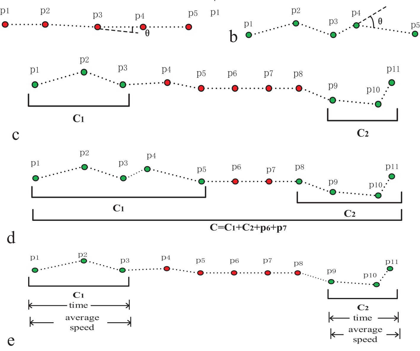
Figure 2. Schematic diagram of the SDB-SMOT algorithm. (a) Non-fishing points (red). (b) Fishing points (green). (c) The sub-trajectory contains two clusters $(n>maxTol)$. (d) The cluster $C_1$,$C_2$, and points between the clusters are merged into one cluster $(n\le maxTol)$. (e) Checking the time and average speed of all clusters.

The steps of the algorithm are as follows:

The fishing vessel trajectory points are represented as $T=\{p_1,p_2,\dots ,p_N\},$ setting the empty set $C.$

Step 1. Select the unvisited point $p_i$ by time series, calculate the difference of the course over ground $DC$ between $p_i$ and $p_{i-1},$ if $DC$ is greater than the direction threshold $minDC$ mark $p_i$ as a fishing point and put it into set $C.$ Repeat Step 1.

Step 2. If $DC$ is less than the direction threshold $minDC,$ and $C$ is not an empty set, then find the set of points with consecutive direction changes less than the threshold among the subsequent points, and the serial number of the last point in the set is notated as $lastIndex.$ If $lastIndex\le i+maxTol,$ then all the points in the set are labeled as fishing points and put into the set $C.$ Otherwise, empty the set $C.$

Step 3. Start at point $p_{i+maxtol+1},$ repeat the steps above until all points in $T$ have been visited.

Step 4. Check the time length of the consecutive fishing points in $T.$ Keep this sub-trajectory if it exceeds the time threshold and the average speed is within the speed range. Else, clear the fishing point markers in the sub-trajectory.

3.3.3 Fishing behavior detection model

The identification of vessel types typically relies on AIS data. This process involves processing AIS data, extracting relevant characteristics, and applying machine learning or deep learning models for classification. However, vessels that do not engage in fishing activities are excluded from identifying fishing grounds. Therefore, there is no need to examine the types of vessels not used for fishing; instead, the focus should be on the vessels in fishing or proximal to fishing activities.

In vessels of unknown types, length of vessel is a typical feature between fishing vessels and other vessels. In the South China Sea, few fishing vessels are longer than 100 meters. Therefore, length checks are carried out on vessels of unknown types. In order to identify fishing grounds from AIS data containing vessels of unknown types, we use a fishing behavior detection model. This model is employed to identify fishing points before identifying fishing grounds. Only trajectories that are considered to be in the state of fishing are used to extract the fishing grounds. For vessels of unknown types, if their trajectories pass the detection criteria of the fishing behavior detection model, it indicates that they have fishing trajectories. We consider these ships to be fishing vessels. The uncertainty analysis regarding the fishing detection model is illustrated in Section 5. As a result, the fishing behavior detection model is built as shown below (Equation 9):

$\begin{array}{ll}{Q}_{ik}=\{\begin{array}{l}1,p_{ik}\text{ is fishing point \&\& }lengthofi<100m\\ 0,\text{ otherwise}\end{array}& (9)\end{array}$

In Equation 9, $Q_{ik}$ is the state of the vessel $i$ at the $k\text{th}$ point ($Q_{ik}=1$ indicates the fishing state of the fishing vessel; otherwise, the vessel is a non-fishing vessel or in a non-fishing state).

3.4 Fishing grounds identification

3.4.1 OPTICS algorithm

This paper uses the clustering method to identify fishing grounds. The OPTICS algorithm is a density-based clustering algorithm (Ankerst et al., 1999), which improves the traditional DBSCAN algorithm. A critical distinction between OPTICS and DBSCAN is that OPTICS is designed to be less sensitive to the initial threshold settings, making it more robust in various applications. OPTICS algorithm does not explicitly generate clusters but generates an ordering of points, representing the density-based clustering structure of the sample points, as shown in Figure 3. The clustering results based on hyperparameters can be obtained from ordering points using a specific formula.

Figure 3

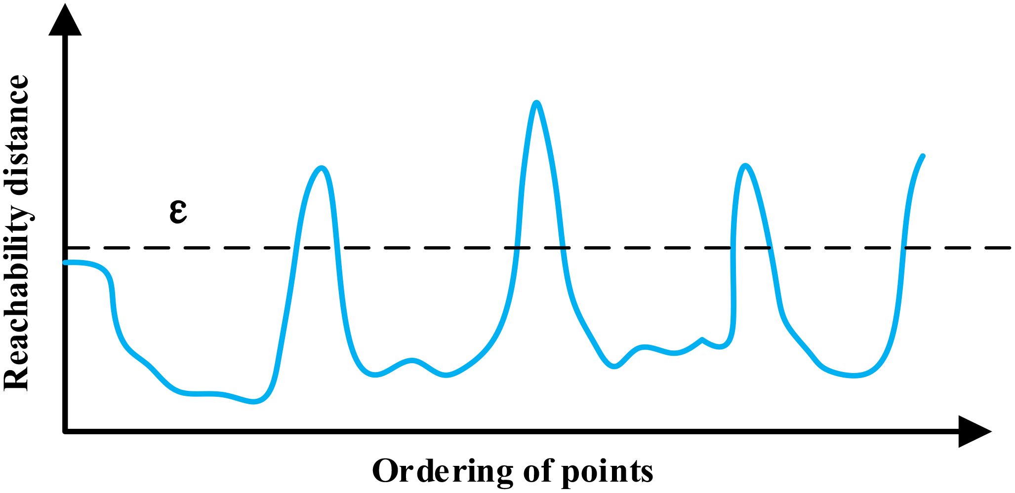
Figure 3. Reachability plot.

The mainly related definitions of the OPTICS algorithm are as follows:

Definition 1: The neighbor of the sample points is defined as follows (Equation 10):

$\begin{array}{ll}{N}_{ϵ}(i)=\{i\in D|dist(i,j)\le ϵ\}& (10)\end{array}$

In Equation 10, $dist(i,j)$ is the distance between the point $i$ and point $j,$ $ϵ$ is the distance threshold.

Definition 2: For a sample point $i\in D,$ if the neighbor $ϵ$ of $i$ satisfies $N_{ϵ}(i)\ge Minpts,$ the point $i$ is called the core point, and the distance between the $Minpts\text{th}$ point in the point $i\text{'}s$ neighbor $ϵ$ and point $i$ is called the core distance, denoted as $coredistance(i)$. where $N_{ϵ}(i)$ is the number of sample points contained in the $ϵ$ of point $i,$ $Minpts$ is the number of sample points threshold.

Definition 3: For a sample point $i\in D,$ the reachability distance from $j$ to $i$ is denoted as follows (Equation 11):

$\begin{array}{ll}reachabilitydistance(i,j)=\{\begin{array}{c}undefined\\ max(coredistance(i),dist(i,j))\end{array}\begin{array}{c},N_{ϵ}(i)<Minpts\\ ,N_{ϵ}(i)\ge Minpts\end{array}& (11)\end{array}$

In Equation 11, $dist(i,j)$ is the distance between point $i$ and point $j.$Definition 4: The points are clustered sequentially. The principle of clustering based on the ordering of points is shown as follows (Equation 12):

$\begin{array}{ll}\mathrm{point}i\{\begin{array}{l}\text{is part of current cluster, }reachabledistance\le ϵ\\ \text{is noise, }coredistance>ϵ\&reachabledistance>ϵ\\ \text{is part of new cluster, }coredistance<ϵ\&reachabledistance>ϵ\end{array}& (12)\end{array}$

In order to improve the performance of clustering algorithms on large-scale trajectory data, the concept of DF (Wang et al., 2014) is introduced. The DF theory is used to describe the non-contact interaction between material particles. Each data object is regarded as a particle with a certain mass in space, around which a virtual action field exists, and any other object located within the field will be subject to the action of the field force. Thus, the joint action of all the objects determines a data field in space.

The definition of the data field is shown as follows: Assuming that there is a data set $D=\left\{x_1,x_2,\dots ,x_n\right\}$ containing $n$ objects, and the resulting data field, $dist(x_i,x_j)$ denotes the Euclidean distance between the objects. $\sigma$ is used to control the interaction force between the objects, and is called the influence factor. In this paper, the average core distance is used as the interaction force range between the objects, and $\sigma$ is set to $averge(coredistance)/3,$ because the value of the Gaussian Kernel function will decay almost to 0 beyond a distance of 3 $\sigma .$ $m_i$ represents the quality of the object $x_i$, i.e., the influence of the object in the data field space. The potential value is expressed as the ordering of points is shown as follows (Equation 13):

$\begin{array}{ll}\phi (x_i)=\frac{1}{n}{\displaystyle \sum _{j=1}^n{m}_i{e}^{-{\left(\frac{dist(x_j,x_i)}{\sigma }\right)}^2}}& (13)\end{array}$

$m_i$ satisfies the normalization condition ${\displaystyle \sum _{i=1}^n{m}_i}=1,$ then the potential value of any point $x_i$ in the space can be expressed as follows (Equation 14)

$\begin{array}{ll}\phi (x_i)=\frac{1}{n}{\displaystyle \sum _{j=1}^n{e}^{-{\left(\frac{dist(x_j,x_i)}{\sigma }\right)}^2}}& (14)\end{array}$

3.4.2 DF-OPTICS algorithm

DF-OPTICS algorithm has the same definitions as the traditional OPTICS algorithm. According to the DF theory, if multiple data objects exist in the data field space with no external force, the data objects will move in opposite directions due to their interactions. The DF potential function is used to react to the size of the interaction force between the data objects in the data field space. A higher value indicates a more significant interaction force from the surrounding trajectory points, indicating a denser concentration of these points. An improved OPTICS algorithm that integrates the DF theory and the DF-OPTICS algorithm is proposed.

The OPTICS algorithm determines the next data point by calculating and updating the reachability distance. It calculates and sorts the reachability distances of neighboring points from the same core point for large-scale and high-density data. However, the minimum value may correspond to multiple neighboring points, posing a problem in selecting the next data point. Figure 4 shows the potential plot and reachability plot. The potential plot has the exact ordering of points with the reachability plot. There is an almost entirely negative correlation between reachability distance and potential value. Hence, the DF theory is crucial in solving this problem. When there are multiple candidate data points in OPTICS, the size of the potential value of these candidate points is calculated, and the object with the highest potential value is chosen as the next data point. This approach ensures that denser trajectory points are prioritized in the ordering of points. The detailed clustering process is shown in Figure 5.

Figure 4

Figure 4. Reachability plot and potential plot (the data from the 2020 AIS data on fishing vessels). (a) Reachability Plot. (b) Potential Plot.

Figure 5

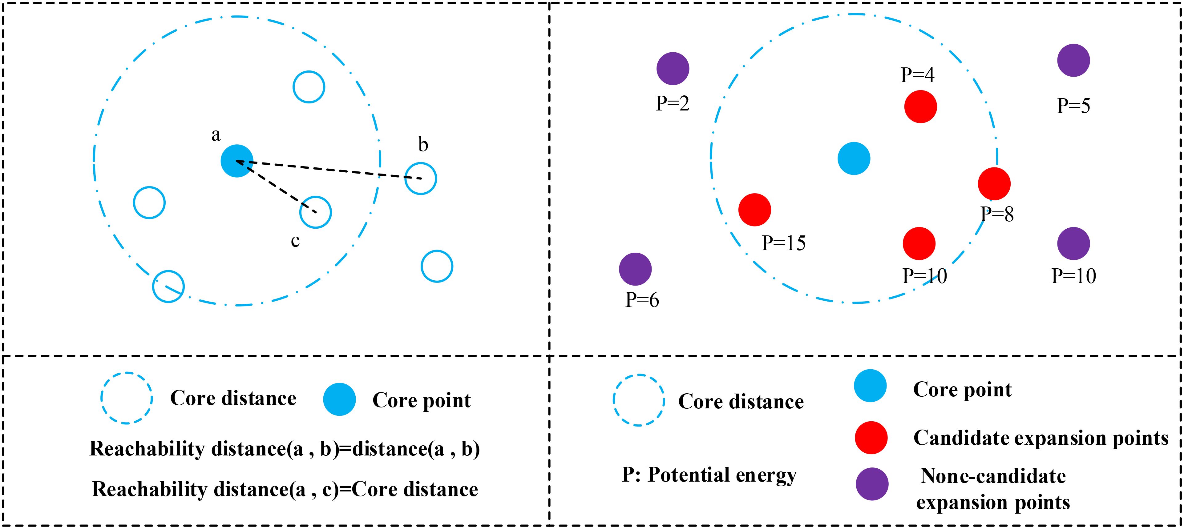
Figure 5. Schematic diagram of the DF-OPTICS algorithm.

The flowchart of the DF-OPTICS algorithm is shown as follows (Algorithms 1–3):

Algorithm 1. Algorithm 1. DF-OPTICS ($D$, $ϵ$ = Inf, Minpts).

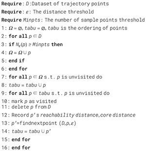
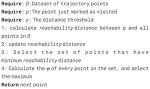
Algorithm 2. findnextpoint ($D$, $p$, $ϵ$).

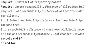
Algorithm 3. update reachability distance.

3.4.3 Fishing grounds identification model

The DF-OPTICS algorithm solves the problem of selecting extension points on large-scale trajectory datasets and effectively improves clustering performance. Due to the DF-OPTICS’ characteristics, large-scale AIS data becomes a suitable application object. The fishing grounds identification model can be built as shown below (Equation 15):

$\begin{array}{ll}{S}_p=\{\begin{array}{l}1,p\in clusters\\ 0,p\in noise\end{array}& (15)\end{array}$

In Equation 15, $S_p$ is the area the point $p$ located in ($S_p=1$ indicates the fishing ground; otherwise, the point is in non-fishing ground).

4 Results

This study examines changes in the South China Sea fishing grounds every quarter in 2020. The fishing grounds are displayed on the electronic nautical charts, which is a data model that describes geographic information.

4.1 The results of fishing behavior detection

The server environment is shown in Table 1.

Table 1

Table 1. The server environment.

The result of the fishing vessel speed distribution map, generated using the GMM model, is shown in Figure 6a. The fishing vessel speed in the South China Sea exhibits a roughly bimodal distribution, which can be interpreted as a mixture of two Gaussian curves corresponding to the fishing operation behaviors (low-speed) and sailing behaviors (high-speed), respectively. By applying the EM algorithm and statistical analysis of the Gaussian curves related to fishing operation behaviors, the average speed of fishing vessels during fishing operations is approximately 2.8 kn, with a standard deviation of approximately 0.8 kn. The confidence interval for the speed associated with fishing operations is calculated as the mean value plus or minus the 1.5 times standard deviation, i.e., 1.6 - 4.0 kn is defined as the range of fishing speeds for fishing vessels (Chen et al., 2022). The log-likelihood function for each iteration is presented in Figure 6b and used to judge convergence. It is clear that the algorithm has reached convergence within the initial 30 iterations.

Figure 6

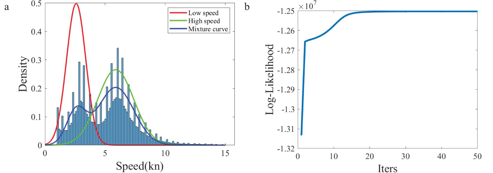
Figure 6. The results of the EM algorithm. ${\varpi }_{low}=0.2379,$ ${\varpi }_{high}=\mathrm{0.7621.}$ (a) Speed distribution of fishing vessels based on the GMM. (b) Log-likelihood function.

Figure 7 presents the results of different fishing behavior detection models. The trajectory is sourced from a fishing vessel with the MMSI number 412300398. The GMM model does not account for the continuity between points. There are a few course changes at the beginning of the trajectory. It can be seen that this method relying solely on a speed threshold is incapable of accurately and continuously identifying fishing behavior.

Figure 7

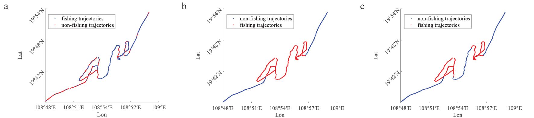
Figure 7. Different methods of fishing behavior detection (the red points represent the fishing trajectory). (a) GMM. (b) DB-SMOT algorithm. (c) SDB-SMOT algorithm.

The difference in the results between the DB-SMOT algorithm and our proposed method is shown in the middle of the two fishing trajectories (Figure 7). Despite some course changes in the middle trajectory, the speed, according to the actual AIS data, significantly exceeds the threshold necessary for fishing activities. However, the DB-SMOT algorithm mistakenly identifies this as a fishing trajectory, indicating a limitation in its approach. As shown in Figure 7, our proposed method, the SDB-SMOT algorithm, is more accurate than the other two methods and can continuously identify fishing trajectories.

To evaluate the effectiveness of the SDB-SMOT algorithm in excluding non-fishing vessels from AIS data that contains vessels of unknown types, this study uses known ship types to illustrate analysis of the model about speed, course and length. If the fishing behavior detection model has a low recognition rate for the trajectories of non-fishing vessels and also can accurately identify fishing behavior in the trajectories of fishing vessels, then the model is considered effective. We take four types of ship as examples to make the process of the model more intuitively explained. In this experiment, these known types are treated as unknown, and the SDB-SMOT algorithm is applied to test its performance. This paper selects trajectories of four known ship types-fishing ship, bulk carrier, liquid cargo carrier, and passenger ship-to demonstrate the model’s effectiveness. The definition of suspected fishing trajectories is based on the visual appearance of the trajectory, which has frequent course changes and the length of ship is less than 100 meters, suggesting it could be a fishing trajectory.

In Figure 8a, the trajectory identified as fishing behavior is marked by red points. It meets the model’s length, speed, course, and duration requirements, indicating that the fishing behavior detection model can effectively identify fishing trajectories from AIS data containing vessels of unknown types. The part of trajectories in Figure 8b seem to display characteristics of fishing behavior and its length is less than 100 meters. Therefore, it is defined as suspected trajectory. However, the bulk carrier in this figure sailed a long distance, almost across the entire South China Sea. Despite the relatively short course change time, it does not meet the fishing activity duration required by the model. Therefore, they are not identified as fishing trajectories by the SDB-SMOT algorithm. The trajectories in Figure 8c seem to exhibit characteristics of fishing behavior; however, the length of this ship is more than 100 meters, so this ship is directly excluded as a fishing vessel by the fishing behavior detection model. Meanwhile, the average speed of the green-marked trajectory is close to zero, suggesting that this trajectory likely represents a vessel that is entering or leaving the port (Yang et al., 2021). In Figure 8d, the trajectory is notably straight, leading to the conclusion that the fishing behavior detection model did not identify any fishing activity trajectories.

Figure 8

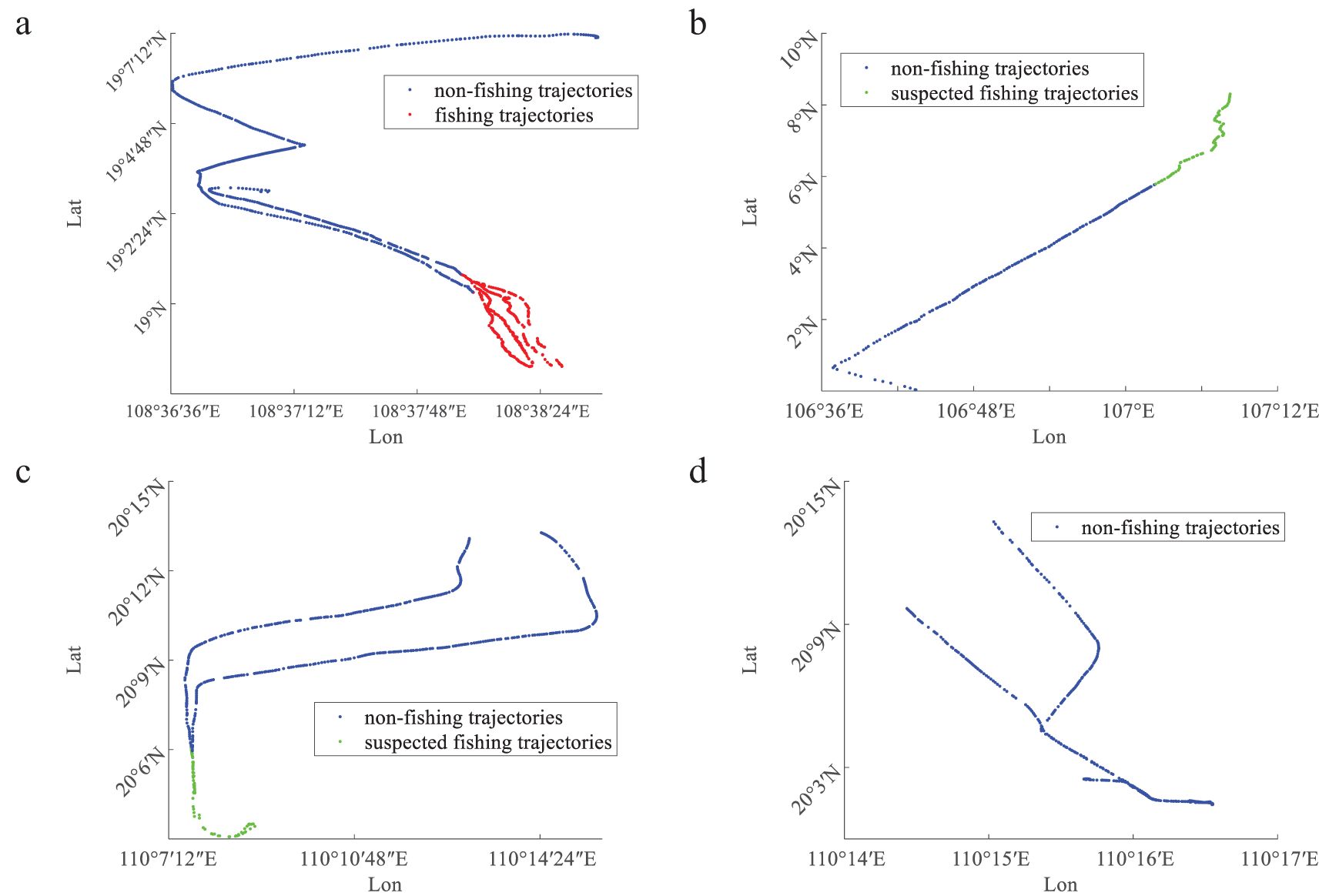
Figure 8. Illustration of SDB-SMOT algorithm from different ship types (Red points represent the fishing trajectory. Green points represent suspected fishing vessel trajectory). (a) Fishing ship MMSI:412340162; Length: 26 meters. (b) Bulk carrier MMSI: 413812238; Length: 68 meters. (c) Passenger ship MMSI: 413233630; Length: 127 meters. (d) Liquid cargo carrier MMSI: 413232860; Length: 95 meters.

Figure 9 presents the results obtained through the fishing behavior detection model using the AIS data from four quarters as an illustrative example. The year is divided into four quarters on average, each quarter corresponds to three months, the first quarter corresponds to January, February, March, the second quarter corresponds to April, May, June, the third quarter corresponds to July, August, September, and the fourth quarter corresponds to October, November, and December. A comparison between Figures 9, 10 reveals that numerous distinct straight-line sailing trajectories have been effectively removed. At the same time, the primary fishing grounds of the fishing vessels have been preserved. This indicates that the algorithm effectively filters out non-fishing activities, which in turn allows for a more focused analysis of the main fishing areas.

Figure 9

Figure 9. The fishing trajectories of fishing vessels detected by the fishing behavior detection model. (a) The first quarter. (b) The second quarter. (c) The third quarter. (d) The fourth quarter.

Figure 10

Figure 10. The original trajectories of fishing vessels. (a) The first quarter. (b) The second quarter. (c) The third quarter. (d) The fourth quarter.

4.2 Clustering performance of different algorithms

A great clustering algorithm can identify clusters and noise more accurately. To analyze the efficacy and effectiveness of the improved clustering algorithm, its performance is measured against three clustering indexes: SC, CHI, and DBI (Equations 16–18). The SC (Bagirov et al., 2023) evaluates the model’s performance using the distance between points within the same cluster and between a point in a neighboring cluster and all other points. The SC ranges from -1 to 1, with values closer to 1 indicating better clustering performance. On the contrary, the closer the value is to -1, the worse the clustering performance is. The formula is as follows (Equation 16):

$\begin{array}{ll}S(i)=\frac{b(i)-a(i)}{max\{a(i),b(i)\}}& (16)\end{array}$

In Equation 16, $a(i)$ represents intra-cluster dissimilarity and $b(i)$ represents inter-cluster dissimilarity.

The CHI (Solorio-Fernández et al., 2016) is primarily based on the ratio between intra-cluster and inter-cluster variance. The higher the value, the better the clustering result. It takes a value in the range of $(0,+\infty ).$ The formula is as follows (Equation 17):

$\begin{array}{ll}CHI=\frac{Tr(B_K)}{Tr(W_K)}*\frac{N-K}{K-1}& (17)\end{array}$

In Equation 17, $K$ denotes the number of categories, $N$ denotes the number of data, $B_K$ is the intergroup discretization matrix, and $W_K$ is the intragroup discretization matrix.

The DBI (Liu et al., 2011) is calculated based on the tightness within clusters and the separation between clusters, with smaller values indicating better results. The value range is [0,1], and the formula is as follows (Equation 18):

$\begin{array}{ll}DBI=\frac{1}{n}{\displaystyle \sum _{i=1}^n\underset{i\ne j}{\max }(}\frac{\overline{S_i}+\overline{S_j}}{{\Vert w_i-w_j\Vert }_2})& (18)\end{array}$

In Equation 18, where $n$ denotes the number of categories, $S$ denotes the average distance within a cluster, and $w$ denotes the cluster center of mass coordinates.

This paper compares our proposed algorithm: DF-OPTICS, with the OPTICS algorithm, DBSCAN algorithm, and an improved OPTICS algorithm. The algorithms’ performances are assessed using three kinds of clustering evaluation indexes, SC, DBI, and CHI, using hyperparameters divided into three cases. Random and consecutive five-month fishing vessels’ AIS data are selected as the test data. The calculation of indexes is executed after deleting the noise. The results represent the average value obtained from each case, as shown in Table 2.

Table 2

Table 2. Clustering evaluation indexes.

Case 1: $Minpts=$ 600; Case 2: $Minpts=$ 800; Case 3: $Minpts=$ 1000. $ϵ$ is set to ten hyperparameters selected randomly in the range of (10000, 20000). In the improved OPTICS algorithm, the minimum cluster size is set to 0.5% of the entire dataset, and the ratio for a significant separation is set to 0.8 (Sander et al., 2003).

The lower the DBI index, the higher the CHI index and SC, and the better the clustering performance. The DF-OPTICS algorithm’s SC and CHI typically outperform those of the other three algorithms across most hyperparameters. Moreover, the DBI index differs significantly from the other three algorithms. Although the improved OPTICS algorithm performs better under specific hyperparameters, its clustering performance is not stabilized. Overall, the clustering performance of the improved OPTICS algorithm is better than the other three clustering algorithms. Better clustering performance can facilitate the identification of more accurate fishing grounds.

4.3 Identifying fishing grounds from AIS data

Figure 11 shows the reachability plot of DF-OPTICS, from which different results can be obtained. We set $Minpts$ as 500 and $ϵ$ as 6000 (meters). Figure 12 presents the fishing grounds identified from AIS data containing fishing vessels and parts of fishing grounds identified from AIS data containing vessels of unknown type.

Figure 11

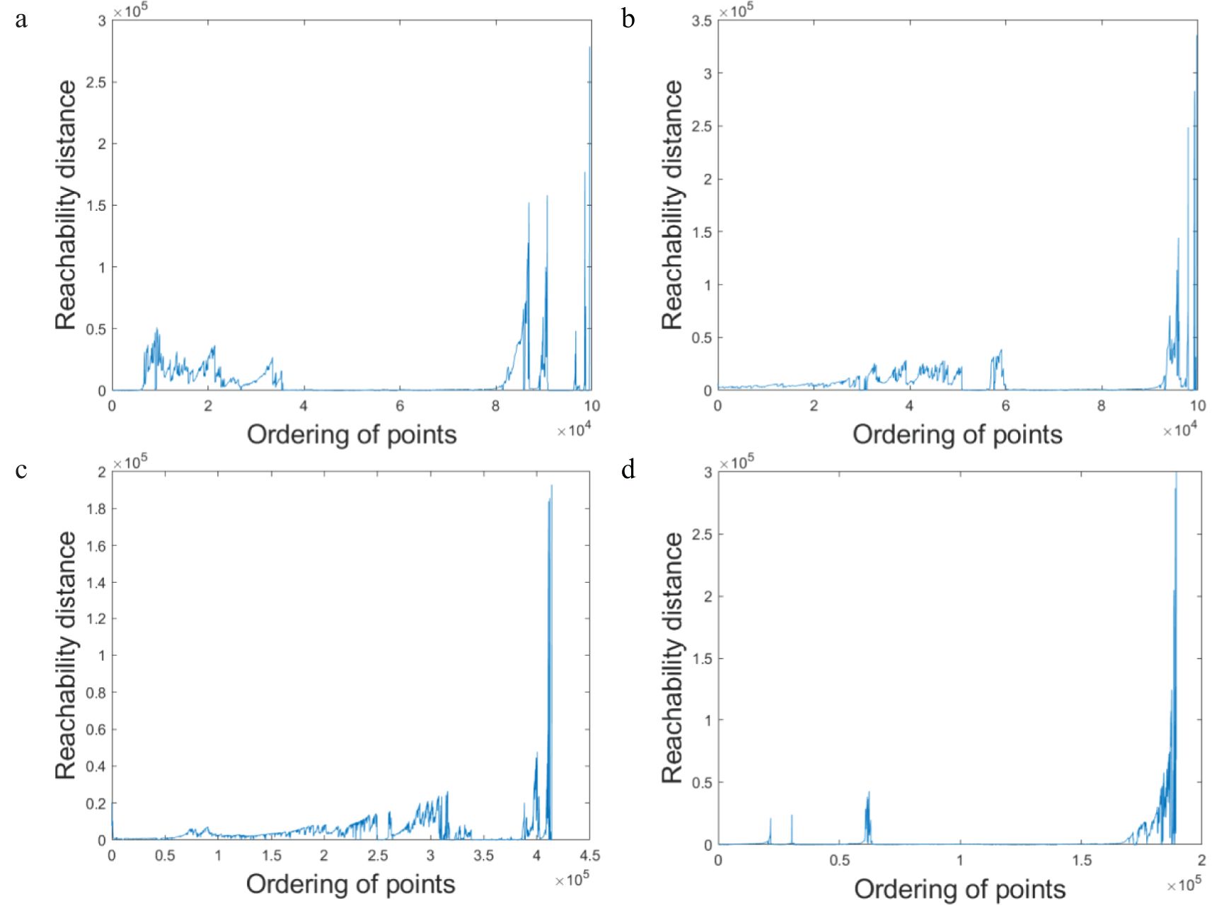
Figure 11. Reachability plot of DF-OPTICS algorithm in different quarters. (a) The first quarter. (b) The second quarter. (c) The third quarter. (d) The fourth quarter.

Figure 12

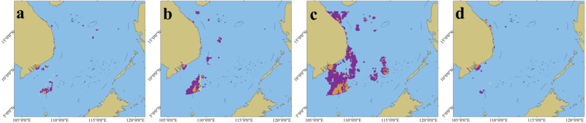
Figure 12. The results of superimposition (The purple area represents the clustering results of known fishing vessels. The yellow area represents the clustering results of fishing vessels extracted from unknown types of vessels). (a) The first quarter. (b) The second quarter. (c) The third quarter. (d) The fourth quarter.

To identify potential fishing grounds from AIS data involving vessels of unknown types, this study overlays the clustering results of unknown ships onto the respective fishing grounds for each quarter. The trajectories of unknown vessels first be detected by the fishing vessel behavior detection model, then the results are obtained based on the fishing grounds extraction model. The visual representation of these findings is presented in Figure 12. The yellow segments represent the results for vessels of unknown types, while the purple segments represent the fishing grounds extracted from known fishing vessels for each quarter. The clustering results for vessels of unknown types are highly coincident with the known fishing grounds. From this, it can be concluded that applying this framework to vessels of unknown types to identify new fishing grounds is a practical approach.

4.4 Spatio-temporal characterization of fishing grounds in the South China Sea

Figure 13 presents the fishing grounds identified through the fishing grounds identification model from AIS data containing vessels of unknown types. The results reveal distinct quarterly variations in the spatial and temporal characteristics of fishing vessel activities in the South China Sea.

Figure 13

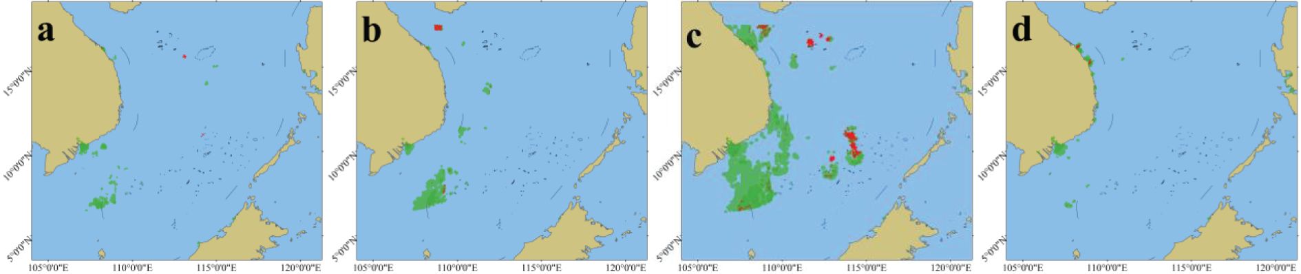
Figure 13. The hot spots of Chinese (red) and other national (green) fishing vessels. (a) The first quarter. (b) The second quarter. (c) The third quarter. (d) The fourth quarter.

In the first quarter, the focal point of these activities is predominantly positioned on the southwest continental shelf of the Nansha Islands, forming a block-like distribution. There is also a minor concentration to the south of the Zhongsha Islands and between the Wave Reefs and the Xisha Islands, covering a total area of approximately 12,738.89 square kilometers. The primary center of fishing activities is positioned southwest of the Nansha Islands.

In the second quarter, a slight increase is noted in the hotspot of fishing activities around the Sansha Islands, with the total area expanding to roughly 43,234.85 square kilometers. The center of gravity for these activities remains essentially unchanged.

In the third quarter, a peak in fishing activities within the South China Sea is observed, characterized by the most extensive range of fishing grounds, the most significant area, and the highest number of hotspots, amounting to a total of 116,508.35 square kilometers. The most considerable fishing ground is located in the southwest of the Nansha Islands. The fishing grounds are primarily distributed in a north-south strip along the Mekong River estuary and the western and central parts of the Nansha Islands. Notably, the Xisha Islands and the southwestern parts of the Nansha Islands exhibit a more fragmented distribution pattern.

In the fourth quarter, fishing activities by vessels in the South China Sea are significantly reduced. There are virtually no aggregation areas for fishing vessels in the Nansha Islands, with only a few small aggregation areas in the Xisha Islands and the southwest regions of the Nansha Islands. These areas cover approximately 2,141 square kilometers.

Based on the analysis above, a consistent hotspot for fishing vessel activities is observed throughout the year on the southwest side of the Nansha Islands. Additionally, the third quarter experiences an increase in aggregation areas for fishing vessels, notably within the Zhongsha, Xisha, and the central regions of the Nansha Islands.

The hotspots of fishing vessels, categorized by their MID numbers that represent different countries and regions, are shown in Figure 13. Notably, fishing vessel activities in the South China Sea have significantly increased during the third and fourth quarters. The primary reason for this increase is the presence of fishing vessels from Southeast Asian countries fishing in the South China Sea (Gou and Yang, 2023).

5 Conclusion

This study proposes a novel framework to identify fishing grounds from AIS data that encompasses vessels of unknown types. This framework covers a fishing behavior detection model and a fishing grounds identification model. Additionally, this framework has been used to analyze the fishing grounds in the South China Sea for the year 2020. The research contributions are as follows:

1. A fishing behavior detection model based on the SDB-SMOT algorithm is proposed. Compared to other methods, the SDB-SMOT algorithm can more precisely identify fishing trajectories from AIS data containing vessels of unknown types. Moreover, the model for fishing behavior can filter out non-fishing vessels from the AIS data containing vessels of unknown types.

2. A fishing grounds identification model is proposed based on the DF-OPTICS algorithm, which solves the problem of identifying the next data point among the points with the same reachability distance in large-scale data for the OPTICS algorithm. The DF-OPTICS algorithm is proven to have better clustering performance on large-scale datasets. It outperforms three other clustering algorithms, the traditional OPTICS algorithm, the DBSCAN algorithm, and the improved OPTICS algorithm, in terms of overall clustering effectiveness. This model is particularly well-suited for identifying the fishing grounds from large-scale and high-density trajectory datasets. It can also reflect the distribution of the fishing grounds more intuitively.

3. Applying this framework to AIS data involving vessels of unknown types has proven to be practical, as it effectively identifies fishing grounds that are in close agreement with the areas previously identified from AIS data containing specified and known fishing vessels. Using this proposed framework, this study examines the fishing grounds in the South China Sea and analyzes their features.

6 Discussion

In order to validate the effects of excluding non-fishing vessels’ trajectories and detecting fishing vessels from unknown vessels, a portion of AIS data from known vessels—including fishing vessels, passenger ships, oil tankers, cargo carriers, and working vessels—are selected to evaluate the fishing behavior detection model. Considering that there are hardly any fishing vessels in the South China Sea that exceed 100 meters in length (Sun et al., 2023), we exclude vessels longer than 100 meters from the AIS data before applying the fishing vessel behavior detection model. The results are shown in Table 3, where ‘Number of FT’ represents the number of AIS data points identified as fishing trajectories. It can be observed that trajectories of vessels other than fishing vessels are less likely to be identified as fishing behavior – For all other ship types, the misidentification rate is below 1.5%. The proportion of oil tankers is very low, because the vast majority of oil tankers are longer than 100 meters. A small amount of data has little impact on the extraction of fishing grounds.

Table 3

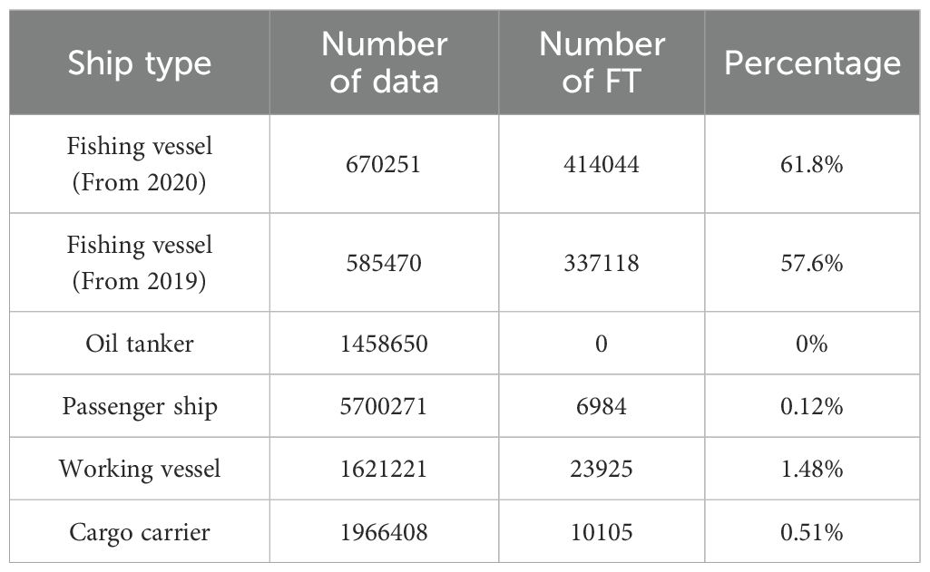
Table 3. The validation of the fishing behavior detection model.

Due to the relatively high percentage of passenger ships and working vessels, this paper presents the hotspots of passenger ships and working vessels in the South China Sea, as shown in Figure 14, and their distribution is quite different from that of fishing grounds. Therefore, we believe that the impact of such vessels is of minor significance with respect to the aim of identifying fishing grounds.

Figure 14

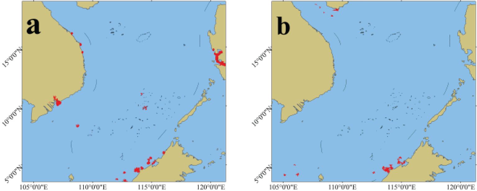
Figure 14. The hotspots of passenger ships and working vessels. (a) The hotspots of passenger ships. (b) The hot spots of working vessels.

A number of vessels have similar or almost identical behavior to fishing behavior, especially those that are more maneuverable and smaller. However, such behaviors are relatively rare and are not typical of them. As shown in Table 3, a low proportion of other vessels are identified by the fishing behavior detection model. While these detected fishing trajectories could potentially influence our findings, we believe the impact is manageable when identifying fishing grounds. Consequently, the fishing behavior detection model may not be fully applicable to a large number of atypical ship behaviors. One of the primary objectives of identifying fishing grounds is to facilitate the prevention of collisions between commercial and fishing vessels.

This paper visually presents the fishing grounds in the South China Sea, which are typically located far from mainland areas and are predominantly witnessed by medium to large fishing vessels. The DF-OPTICS algorithm, integrated with the DF theory, increases the computational complexity due to its need to calculate the potential value of trajectory points. Future research may develop more accurate algorithms for identifying fishing trajectory points while optimizing the time complexity of the DF-OPTICS algorithm.

This paper uses AIS data as the basis for the fishing grounds identification study, and it is impossible to identify the trajectories of fishing vessels without AIS equipment or with AIS equipment turned off, which is a shortcoming of this study. Examining the activity areas of fishing vessels is significant for studying maritime safety and management. However, fishing vessel activity areas are not limited to fishing grounds; for example, fishing ports play a crucial role. Future research may also focus on discovering fishing ports from fishing vessels’ trajectory data.

Data availability statement

The datasets presented in this article are not readily available because the data were procured from LoongShip Corporation, LTD (https://www.loongship.com) and Shanghai Maili Marine Technology Company (https://www.hifleet.com/) and are not publicly available due to commercial contractual restrictions. Requests to access the datasets should be directed to Y3NAbG9vbmdzaGlwLmNvbQ==; c2FsZXNAaGlmbGVldC5jb20=.

Author contributions

CH: Conceptualization, Formal Analysis, Funding acquisition, Methodology, Project administration, Resources, Supervision, Validation, Writing – original draft, Writing – review & editing. JK: Investigation, Methodology, Software, Visualization, Writing – original draft. JZe: Conceptualization, Formal Analysis, Funding acquisition, Supervision, Writing – review & editing. YC: Conceptualization, Resources, Writing – review & editing. JZo: Formal Analysis, Supervision, Visualization, Writing – review & editing.

Funding

The author(s) declare that financial support was received for the research and/or publication of this article. This work was supported by the National Natural Science Foundation of China(Grant NO.51909156, 52372416), and the Shanghai Science and Technology Innovation Action Plan (Grant NO.22010501800).

Conflict of interest

The authors declare that the research was conducted in the absence of any commercial or financial relationships that could be construed as a potential conflict of interest.

Generative AI statement

The author(s) declare that no Generative AI was used in the creation of this manuscript.

Publisher’s note

All claims expressed in this article are solely those of the authors and do not necessarily represent those of their affiliated organizations, or those of the publisher, the editors and the reviewers. Any product that may be evaluated in this article, or claim that may be made by its manufacturer, is not guaranteed or endorsed by the publisher.

References

Agrawal K. P., Garg S., Sharma S., Patel P. (2016). Development and validation of OPTICS based spatio-temporal clustering technique. Inf. Sci. 369, 388–401. doi: 10.1016/j.ins.2016.06.048

Crossref Full Text | Google Scholar

Alemany D., Acha E. M., Iribarne O. O. (2014). Marine fronts are important fishing areas for demersal species at the Argentine Sea (Southwest Atlantic Ocean). J. Sea Res. 87, 56–67. doi: 10.1016/j.seares.2013.12.006

Crossref Full Text | Google Scholar

Ankerst M., Breunig M. M., Kriegel H.-P., Sander J. (1999). OPTICS: ordering points to identify the clustering structure. ACM SIGMOD Rec. 28, 49–60. doi: 10.1145/304181.304187

Crossref Full Text | Google Scholar

Bagirov A. M., Aliguliyev R. M., Sultanova N. (2023). Finding compact and well-separated clusters: Clustering using silhouette coefficients. Pattern Recognit. 135, 109144. doi: 10.1016/j.patcog.2022.109144

Crossref Full Text | Google Scholar

Campos A., Leitão P., Sousa L., Gaspar P., Henriques V. (2023). Spatial patterns of fishing activity inside the Gorringe bank MPA based on VMS, AIS and e-logbooks data. Mar. Policy 147, 105356. doi: 10.1016/j.marpol.2022.105356

Crossref Full Text | Google Scholar

Cappa P., Andreoli V., Krueger K., Barrie S., La C., Zeller D. (2024). Estimating fisheries catch from space: Comparing catch estimates derived from AIS fishing effort with reported catches for Indian Ocean industrial fisheries. Reg. Stud. Mar. Sci. 77, 103632. doi: 10.1016/j.rsma.2024.103632

Crossref Full Text | Google Scholar

Chen X., Dou S., Song T., Wu H., Sun Y., Xian J. (2024). Spatial-temporal ship pollution distribution exploitation and harbor environmental impact analysis via large-scale AIS data. J. Mar. Sci. Eng. 12, 960. doi: 10.3390/jmse12060960

Crossref Full Text | Google Scholar

Chen D., Wang X., Li Y., Lang J., Zhou Y., Guo X., et al. (2017). High-spatiotemporal-resolution ship emission inventory of China based on AIS data in 2014. Sci. Total Environ. 609, 776–787. doi: 10.1016/j.scitotenv.2017.07.051

Crossref Full Text | Google Scholar

Chen R., Wu X., Liu B., Wang Y., Gao Z. (2022). Mapping coastal fishing grounds and assessing the effectiveness of fishery regulation measures with AIS data: A case study of the sea area around the Bohai Strait, China. Ocean Coast. Manage. 223, 106136. doi: 10.1016/j.ocecoaman.2022.106136

Crossref Full Text | Google Scholar

Chuaysi B., Kiattisin S. (2020). Fishing vessels behavior identification for combating IUU fishing: enable traceability at sea. Wirel. Pers. Commun. 115, 2971–2993. doi: 10.1007/s11277-020-07200-w

Crossref Full Text | Google Scholar

Coello J., Williams I., Hudson D. A., Kemp S. (2015). An AIS-based approach to calculate atmospheric emissions from the UK fishing fleet. Atmos. Environ. 114, 1–7. doi: 10.1016/j.atmosenv.2015.05.011

Crossref Full Text | Google Scholar

Ferrà C., Tassetti A. N., Grati F., Pellini G., Polidori P., Scarcella G., et al. (2018). Mapping change in bottom trawling activity in the Mediterranean Sea through AIS data. Mar. Policy 94, 275–281. doi: 10.1016/j.marpol.2017.12.013

Crossref Full Text | Google Scholar

Fitrianah D., Hidayanto A. N., Gaol J. L., Fahmi H., Arymurthy A. M. (2016). A spatio-temporal data-mining approach for identification of potential fishing zones based on oceanographic characteristics in the eastern Indian ocean. IEEE J. Sel. Top. Appl. Earth Obs. Remote Sens. 9, 3720–3728. doi: 10.1109/JSTARS.2015.2492982

Crossref Full Text | Google Scholar

Geng R., Liu X., Lv X., Hu X. (2023). Spatial-temporal variation of marine fishing activities responding to policy and social events in China. J. Environ. Manage. 348, 119321. doi: 10.1016/j.jenvman.2023.119321

PubMed Abstract | Crossref Full Text | Google Scholar

Gou Y., Yang C. (2023). Dilemmas and paths of international cooperation in China's fight against IUU fishing analysis. Mar. Policy. 155, 105789. doi: 10.1016/j.marpol.2023.105789

Crossref Full Text | Google Scholar

Gu Y., Hu Z., Zhao Y., Liao J., Zhang W. (2024). MFGTN: A multi-modal fast gated transformer for identifying single trawl marine fishing vessel. Ocean Eng. 303, 117711. doi: 10.1016/j.oceaneng.2024.117711

Crossref Full Text | Google Scholar

Guan Y., Zhang J., Zhang X., Li Z., Meng J., Liu G., et al. (2021). Identification of fishing vessel types and analysis of seasonal activities in the northern south China sea based on AIS data: A case study of 2018. Remote Sens. 13, 1952. doi: 10.3390/rs13101952

Crossref Full Text | Google Scholar

Hu B., Jiang X., Souza E., Pelot R., Matwin S. (2016). doi: 10.15439/2016F546

Crossref Full Text | Google Scholar

Huang C., Qi X., Zheng J., Zhu R., Shen J. (2023). A maritime traffic route extraction method based on density-based spatial clustering of applications with noise for multi-dimensional data. Ocean Eng. 268, 113036. doi: 10.1016/j.oceaneng.2022.113036

Crossref Full Text | Google Scholar

Hutniczak B., Wilson D. T., Stewart I. J., Hicks A. C. (2024). A hundred years of Pacific halibut management in the context of global events and trends in fisheries management. Front. Mar. Sci. 11. doi: 10.3389/fmars.2024.1424002

Crossref Full Text | Google Scholar

James M., Mendo T., Jones E. L., Orr K., McKnight A., Thompson J. (2018). AIS data to inform small scale fisheries management and marine spatial planning. Mar. Policy 91, 113–121. doi: 10.1016/j.marpol.2018.02.012

Crossref Full Text | Google Scholar

Jeon H.-K., Han J. R. (2022). Random forest classifier-based ship type prediction with limited ship information of AIS and V-pass. Korean J. Remote Sens. 38, 435–446. doi: 10.7780/KJRS.2022.38.4.10

Crossref Full Text | Google Scholar

Le Guyader D., Ray C., Gourmelon F., Brosset D. (2017). Defining high-resolution dredge fishing grounds with Automatic Identification System (AIS) data. Aquat. Living Resour. 30, 39. doi: 10.1051/alr/2017038

Crossref Full Text | Google Scholar

Li J., Cai Y., Zhang P., Zhang Q., Jing Z., Wu Q., et al. (2021). Satellite observation of a newly developed light-fishing “hotspot. Open South China Sea Remote Sens. Environ. 256, 112312. doi: 10.1016/j.rse.2021.112312

Crossref Full Text | Google Scholar

Li H., Jia P., Wang X., Yang Z., Wang J., Kuang H. (2023). Ship carbon dioxide emission estimation in coastal domestic emission control areas using high spatial-temporal resolution data: A China case. Ocean Coast. Manage. 232, 106419. doi: 10.1016/j.ocecoaman.2022.106419

Crossref Full Text | Google Scholar

Li J., Qiu Y., Cai Y., Zhang K., Zhang P., Jing Z., et al. (2022). Trend in fishing activity in the open South China Sea estimated from remote sensing of the lights used at night by fishing vessels. ICES J. Mar. Sci. 79, 230–241. doi: 10.1093/icesjms/fsab260

Crossref Full Text | Google Scholar

Li C., Yuan Z., Ou J., Fan X., Ye S., Xiao T., et al. (2016). An AIS-based high-resolution ship emission inventory and its uncertainty in Pearl River Delta region, China. Sci. Total Environ. 573, 1–10. doi: 10.1016/j.scitotenv.2016.07.219

PubMed Abstract | Crossref Full Text | Google Scholar

Liu Y., Wu X., Shen Y. (2011). Automatic clustering using genetic algorithms. Appl. Math. Comput. 218, 1267–1279. doi: 10.1016/j.amc.2011.06.007

Crossref Full Text | Google Scholar

Masroeri A. A., Aisjah A. S., Jamali M. M. (2021). IUU fishing and transhipment identification with the miss of AIS data using Neural Networks. IOP Conf. Ser. Mater. Sci. Eng. 1052, 12054. doi: 10.1088/1757-899X/1052/1/012054

Crossref Full Text | Google Scholar

Mazzarella F., Vespe M., Damalas D., Osio G. (2014).Discovering vessel activities at sea using AIS data: Mapping of fishing footprints. In: 17th international conference on information fusion (FUSION). Available online at: https://ieeexplore.ieee.org/abstract/document/6916045/citations?tabFilter=paperscitations (Accessed March 19, 2024).

Google Scholar

Merchan F., Contreras K., Poveda H., Guzman H. M., Sanchez-Galan J. E. (2024). Unsupervised identification of Greater Caribbean manatees using Scattering Wavelet Transform and Hierarchical Density Clustering from underwater bioacoustics recordings. Front. Mar. Sci. 11. doi: 10.3389/fmars.2024.1416247

Crossref Full Text | Google Scholar

Natale F., Gibin M., Alessandrini A., Vespe M., Paulrud A. (2015). Mapping fishing effort through AIS data. PloS One 10, e0130746. doi: 10.1371/journal.pone.0130746

PubMed Abstract | Crossref Full Text | Google Scholar

Owiredu S. A., Kim K.-I. (2021). Spatio-temporal fish catch assessments using fishing vessel trajectories and coastal fish landing data from around jeju island. Sustainability 13, 13841. doi: 10.3390/su132413841

Crossref Full Text | Google Scholar

Peel D., Good N. M. (2011). A hidden Markov model approach for determining vessel activity from vessel monitoring system data. Can. J. Fish. Aquat. Sci. 68, 1252–1264. doi: 10.1139/f2011-055

Crossref Full Text | Google Scholar

Perez J. A. A., Gavazzoni L., Sant’Ana R. (2024). Historical fishing regimes uncover deep-sea productivity hotspots in the SW Atlantic Ocean. Front. Mar. Sci. 11. doi: 10.3389/fmars.2024.1477960

Crossref Full Text | Google Scholar

Rocha J. A. M. R., Times V. C., Oliveira G., Alvares L. O., Bogorny V. (2010). “DB-SMoT: A direction-based spatio-temporal clustering method,” in 2010 5th IEEE International Conference Intelligent Systems. 114–119 (London, United Kingdom: IEEE). doi: 10.1109/IS.2010.5548396

Crossref Full Text | Google Scholar

Sander J., Qin X., Lu Z., Niu N., Kovarsky A. (2003). “Automatic extraction of clusters from hierarchical clustering representations,” in Advances in knowledge discovery and data mining. Eds. Whang K.-Y., Jeon J., Shim K., Srivastava J. (Springer Berlin Heidelberg, Berlin, Heidelberg), 75–87. doi: 10.1007/3-540-36175-8_8

Crossref Full Text | Google Scholar

Shi Y., Hong F., Zhao Z., Jiang Y., Zhou S., Huang H. (2024a). HyFish: hydrological factor fusion for prediction of fishing effort distribution with VMS dataset. Front. Mar. Sci. 11. doi: 10.3389/fmars.2024.1296146

Crossref Full Text | Google Scholar

Shi Y., Yan L., Zhang S., Tang F., Yang S., Fan W., et al. (2024b). Revealing the effects of environmental and spatio-temporal variables on changes in Japanese sardine (Sardinops melanostictus) high abundance fishing grounds based on interpretable machine learning approach. Front. Mar. Sci. 11. doi: 10.3389/fmars.2024.1503292

Crossref Full Text | Google Scholar

Solorio-Fernández S., Carrasco-Ochoa J. A., Martínez-Trinidad J. Fco. (2016). A new hybrid filter–wrapper feature selection method for clustering based on ranking. Neurocomputing 214, 866–880. doi: 10.1016/j.neucom.2016.07.026

Crossref Full Text | Google Scholar

Sun Y., Lian F., Yang Z. (2023). Analysis of the activities of high sea fishing vessels from China, Japan, and Korea via AIS data mining. Ocean Coast. Manage. 242, 106690. doi: 10.1016/j.ocecoaman.2023.106690

Crossref Full Text | Google Scholar

Tang C., Chen M., Zhao J., Liu T., Liu K., Yan H., et al. (2021). A novel ship trajectory clustering method for Finding Overall and Local Features of Ship Trajectories. Ocean Eng. 241, 110108. doi: 10.1016/j.oceaneng.2021.110108

Crossref Full Text | Google Scholar

Tassetti A. N., Ferrà C., Fabi G. (2019). Rating the effectiveness of fishery-regulated areas with AIS data. Ocean Coast. Manage. 175, 90–97. doi: 10.1016/j.ocecoaman.2019.04.005

Crossref Full Text | Google Scholar

van Geffen A. (2017). Detecting fishing activity and fishing gear types based on spatial- temporal vessel characteristics from AIS data. Netherlands: Tilburg University.

Google Scholar

Wan L., Cheng T., Fan W., Shi Y., Zhang H., Zhang S., et al. (2024). Spatial information extraction of fishing grounds for light purse seine vessels in the Northwest Pacific Ocean based on AIS data. Heliyon 10, e28953. doi: 10.1016/j.heliyon.2024.e28953

PubMed Abstract | Crossref Full Text | Google Scholar

Wang S., Jinghua F., Meng F., Hanning Y. (2014). HGCUDF: hierarchical grid clustering using data field. Chin. J. Electron. 23, 37–42. doi: 10.23919/CJE.2014.10848035

Crossref Full Text | Google Scholar

Welch H., Clavelle T., White T. D., Cimino M. A., Van Osdel J., Hochberg T., et al. (2022). Hot spots of unseen fishing vessels. Sci. Adv. 8, eabq2109. doi: 10.1126/sciadv.abq2109

PubMed Abstract | Crossref Full Text | Google Scholar

Wu W., Zhang P., Wang Q., Kang L., Su F. (2024). Analysis of fishing intensity in the South China Sea based on automatic identification system data: A comparison between China and Vietnam. Mar. Coast. Fish. 16, e10309. doi: 10.1002/mcf2.10309

Crossref Full Text | Google Scholar

Wu S., Zimanyi E., Sakr M., Torp K. (2022). “Semantic segmentation of AIS trajectories for detecting complete fishing activities,” in 2022 23rd IEEE International Conference on Mobile Data Management (MDM). 419–424 (Paphos, Cyprus: IEEE). doi: 10.1109/MDM55031.2022.00092

Crossref Full Text | Google Scholar

Xie W., Li Y., Yang Y., Wang P., Wang Z., Li Z., et al. (2023). Maritime greenhouse gas emission estimation and forecasting through AIS data analytics: a case study of Tianjin port in the context of sustainable development. Front. Mar. Sci. 10. doi: 10.3389/fmars.2023.1308981

Crossref Full Text | Google Scholar

Xing B., Zhang L., Liu Z., Sheng H., Bi F., Xu J. (2023). The study of fishing vessel behavior identification based on AIS data: A case study of the east China sea. J. Mar. Sci. Eng. 11, 1093. doi: 10.3390/jmse11051093

Crossref Full Text | Google Scholar

Yan Z., He R., Ruan X., Yang H. (2022). Footprints of fishing vessels in Chinese waters based on automatic identification system data. J. Sea Res. 187, 102255. doi: 10.1016/j.seares.2022.102255

Crossref Full Text | Google Scholar

Yang D., Wu L., Wang S. (2021). Can we trust the AIS destination port information for bulk ships?–Implications for shipping policy and practice. Transp. Res. Part E Logist. Transp. Rev. 149, 102308. doi: 10.1016/j.tre.2021.102308

Crossref Full Text | Google Scholar

Yang D., Li X, Zhang L. (2024). A novel vessel trajectory feature engineering for fishing vessel behavior identification. Ocean Eng. 310, 118677. doi: 10.1016/j.oceaneng.2024.118677

Crossref Full Text | Google Scholar

Zeng Z., Liu D., Ke L., Zhang S., Liu S. (2024). Machine learning-based analysis of sea fog’s spatial and temporal impact on near-miss ship collisions using remote sensing and AIS data. Front. Mar. Sci. 11. doi: 10.3389/fmars.2024.1536363

Crossref Full Text | Google Scholar

Zhang C., Chen Y., Xu B., Xue Y., Ren Y. (2022). The dynamics of the fishing fleet in China Seas: A glimpse through AIS monitoring. Sci. Total Environ. 819, 153150. doi: 10.1016/j.scitotenv.2022.153150

PubMed Abstract | Crossref Full Text | Google Scholar

Zhang H., Yang S.-L., Fan W., Shi H.-M., Yuan S.-L. (2021). Spatial analysis of the fishing behaviour of tuna purse seiners in the western and central pacific based on vessel trajectory data. J. Mar. Sci. Eng. 9, 322. doi: 10.3390/jmse9030322

Crossref Full Text | Google Scholar