Joint optimization of AoI and energy for AUV-assisted data collection in underwater acoustic sensor networks

Underwater data collection is a key component of ocean observation systems, providing reliable data provenance through sensor networks deployed across diverse marine environments. Timely and energy-efficient data collection mechanisms are critical for ensuring the continuity and integrity of the collected data. For the sake of jointly optimizing the age of information (AoI) and energy consumption, we propose a multi-autonomous underwater vehicle (AUV)-assisted underwater data collection scheme in this paper. The optimization problem is formulated as a mixed integer linear programming (MILP) problem, which is non-deterministic polynomial (NP)-hard. In order to address the problem efficiently, we propose a two-stage method. First, considering the balance of energy consumption and the limitation of sensor communication ranges, we design a cluster-based AUV scheduling data transmission protocol to find a series of hovering points at which the AUVs hover to receive data and schedule data transmissions between the AUVs and sensors. Based on that, a combined heuristic algorithm is proposed to plan AUVs’ trajectories so that the data collection task can be completed properly with a low cost. Simulation results show that the proposed algorithm outperforms three benchmark algorithms in terms of average AoI and collection utility. Specifically, the freshness of information and the collection utility improved by 10.23% and 33.36% on average, respectively. Additionally, the energy consumption of sensor nodes is more balanced, and the network lifetime is extended.

1 Introduction

The ocean is regarded as the second living space for human beings, which covers approximately 70% of the Earth’s surface (National Research Council, Division on Earth, Life Studies, Ocean Studies Board andCommittee on Exploration of the Seas, 2003). Ocean observation and exploration have emerged all over the world. Underwater acoustic sensor networks (UASNs), being a powerful means of ocean observation and exploration, play an increasingly important role in smart oceans. With the development of the internet of underwater things (IoUT), the number of underwater equipment continues to grow rapidly. Massive heterogeneous data are generated underwater such that UASNs have entered the era of big data (Qiu et al., 2019).

Marine information collection is the basic function of UASNs, which supports the data requirements for marine science. However, the inherent characteristics of UASNs bring difficulties to underwater data collection, such as unreliable long-distance communication links, difficulties in replenishing the energy for underwater sensor nodes, and high bit error rates and delays in data transmission (Wang et al., 2019, 2020; Han et al., 2019). Owing to the convenience of power supply, mobility, and stronger computing and communication capabilities, autonomous underwater vehicles (AUVs) have been widely used in UASNs to improve performance (Yang et al., 2021). In general, existing underwater data collection schemes could be divided into two types, namely, multi-hop routing schemes and AUV-assisted schemes (de Souza et al., 2016; Gjanci et al., 2017). On the one hand, the multi-hop routing schemes relay sensed data to the sink node, causing the hot area problem and additional collection delay (Guan et al., 2019; Hwang and Kim, 2008; Li et al., 2016). Most of the existing routing protocols are applied in static networks, without considering the mobility of nodes (Khan et al., 2024, 2023). On the other hand, AUV-assisted underwater data collection schemes that focus on energy efficiency (Zhuo et al., 2020), network throughput (Luo et al., 2022), and multi-AUV collaboration (Han et al., 2021) have attracted increasing attention (Su et al., 2019).

However, few studies have considered optimizing information freshness, i.e., age of information (AoI) (Talak et al., 2018), which is defined as the time interval between when information is sampled and when it is sent to the data center (Kaul et al., 2012), in AUV-assisted underwater data collection schemes. Admittedly, the freshness of the sensed information is a crucial metric that cannot be ignored in delay-sensitive applications. In terrestrial wireless sensor networks (TWSNs), a considerable amount of research about AoI has been studied. In Liu et al. (2020a), an unmanned aerial vehicle (UAV)-aided data collection framework is applied in TWSN to minimize the average AoI and max-AoI. Abd-Elmagid et al. noted that one UAV serves as a mobile relay to optimize the peak AoI from source to destination (Abd-Elmagid and Dhillon, 2018). Zhang et al. (2020) discussed the trade-off between sensing and communication through directly utilizing UAV to sense information in the target area. Unfortunately, the AoI-oriented optimization algorithms in TWSN data collection systems cannot be directly applied to UASNs due to the obvious differences between UASNs and TWSNs.

Motivated by the above-mentioned issues, this paper proposes a multi-AUV-assisted underwater data collection scheme, in which the joint optimization of AoI and energy efficiency is considered. The main contributions of this paper can be summarized as follows:

1. We propose a multi-AUV-assisted data collection scheme (MADCS) for UASNs. Unlike existing solutions, MADCS jointly optimizes the average AoI and energy consumption via determining the AUV hovering positions, the association between the sensor nodes and AUVs, the data transmission protocol, and AUVs’ trajectory.

2. The optimization problem is formulated as a mixed integer linear programming (MILP) problem, which is non-deterministic polynomial (NP)-hard and difficult to solve. To reduce the computational complexity, we solve this problem in two steps. First, we propose a cluster-based AUV scheduling data transmission protocol, in which a canopy-Kmeans (CK) clustering algorithm is applied to establish a cluster-based network topology and an AUV scheduling data transmission protocol is designed to reduce the energy consumption and AoI of sensors. Second, a path planning algorithm named PGS is used to plan traversal trajectories for AUVs, improving the information freshness and collection utility.

3. Sufficient simulations are conducted to evaluate the performance of our proposed scheme, MADCS, compared to the three benchmark algorithms. The simulation results demonstrate the advantages of MADCS, which outperforms the three compared algorithms in terms of average AoI and collection utility. In addition, MADCS balances the energy consumption of sensor nodes and thus extends the network lifetime of UASNs.

The rest of this paper is organized as follows. Section 2 presents related work on AUV-assisted data collection schemes in USANs with a focus on energy efficiency and AoI optimization. Section 3 provides the system model, including the underwater acoustic communication model, the proposed AUV-assisted data collection network, and the derivation of the problem. In Section 4, we introduce the details of the proposed MADCS. Simulation results and analysis are presented in Section 5. Finally, conclusions are drawn in Section 6.

2 Related studies and motivation

Collecting data and transmitting it to the sink node in a timely manner while minimizing the network energy consumption is a critical issue for UASNs. This section reviews previous works on data collection in UASNs.

Traditional underwater data collection schemes are mainly based on multi-hop routing. Low-energy adaptive clustering hierarchy (LEACH) (Heinzelman et al., 2002) combines the energy-efficient cluster-based routing and medium access control together with data aggregation to achieve good performance in terms of system lifetime, latency, and application-perceived quality. LEACH is extended to UASNs in Zhao et al. (2021), where mobile sink LEACH (MS-LEACH) and mobile sink LEACH based on energy and density (MS-LEACH-ED) are proposed to further save energy. In Guan et al. (2019), a distance vector-based opportunistic routing (DVOR) scheme is proposed to establish distance vectors for sensors and develop opportunity routes to forward packets. The authors designed an improved energy optimization clustering algorithm (EOCA) (Yu et al., 2020) for multi-hop acoustic cooperative sensor networks to prolong the network lifetime and maintain good communication performance. A novel chaotic search-and-rescue optimization-based multi-hop data transmission (CSRO-MHDT) protocol for UASNs is introduced in Anuradha et al. (2022). Residual energy, distance, and node degree are taken into account in the fitness function. The number of packets received is improved by the CSRO-MHDT protocol. The authors in ur Rahman et al. (2023) and Rahman et al. (2023) propose a new multi-hop energy-efficient and low-collision MAC protocol using the Q-learning technique for UASNs. By utilizing the Q-learning approach, the protocol is able to make informed decisions in selecting the optimal communication path while minimizing energy consumption and reducing the occurrence of collisions.

Recently, a variety of data collection schemes based on AUVs have been studied. AEEDCO and AEEDCOA are developed in Zhuo et al. (2020), and they solved the energy consumption utility maximization problem in four steps based on a single AUV. Luo et al. (2022) introduced an optical–acoustic hybrid communication network and then maximized network throughput by capturing channel variations and AUV mobility. In order to reduce the task load on a single AUV, a multi-AUV collaborative data collection algorithm is proposed in Han et al. (2021). The algorithm includes multi-AUV task allocation and Q-learning-based path planning that reduces the delay of data collection and leverages the energy consumption of a network. Considering the three-dimensional (3D) UASNs, a stratification-based data collection scheme was proposed in Han et al. (2018). In the upper layer, a forward set-based multi-hop forwarding algorithm is used while a neighbor density clustering-based AUV data-gathering algorithm is applied. Omeke et al. (2021) proposed a distance- and energy-constrained k-means clustering scheme for cluster head selection. The members in the cluster transmit their data to the cluster head, and then a single AUV visits all the clusters to collect data. Hao et al. (2023) proposed a novel AUV-based energy-efficient data collection scheme, in which a new cluster head selection method and a transmission strategy suitable for large-scale AUV-assisted UASNs are utilized to improve energy utility and efficiency. Considering the AUV’s limited energy, the dynamic data upload demand of sensor nodes, and the diminishing value of information during data transmission, Xu et al. (2024) formulated the AUV path planning as a multi-objective optimization problem and employed the deep deterministic policy gradient algorithm to address it.

AoI optimization in underwater data collection is emerging. In Khan et al. (2019), end-to-end data freshness constraint is considered in the design of the AUV traversal path to improve the overall data freshness. With the purpose of minimizing the peak AoI, a multi-AUV-assisted heterogeneous underwater information collection scheme is proposed in Fang et al. (2021), and the limited service M/G/1 vacation queueing model is utilized to model the process of information exchange, where the optimal upper limit of the number of AUVs served in the queueing system and the steady-state distribution of the queue length is derived. An underwater linear network is considered in Al-Habob et al. (2021), where an AUV gathers data from a set of underwater devices. In order to reduce AoI, a deep reinforcement learning-based technique is developed to find the optimal locations of data gathering points as well as the hovering time. To improve the feasibility and practicality of AUV-assisted underwater data collection, the work in Li et al. (2023) used graph attention network to embed the information of ocean currents, time window, and sensor locations into the directed maneuver time–cost graph and then applied proximal policy optimization algorithm to select cluster head sensors and generate AUV routes. Jiang et al. (2024) proposed a target uncertainty map-assisted data collection scheme for AUV swarms based on the multiagent proximal policy optimization algorithm. By leveraging current and past search and collection results, the AUV swarms are guided to areas with higher probabilities of containing sensor nodes. Additionally, AoI is introduced to enable a comprehensive exploration of unknown environments.

As mentioned above, most previous studies have focused on the separate optimization of energy or AoI and rarely considered the joint optimization of them. In this paper, we propose a multi-AUV-assisted underwater data collection scheme.

3 System model

In this article, we consider a multi-AUV-assisted data collection scenario in 3D heterogeneous UASNs, which consists of a data center s₀ located on the sea surface, N sensor nodes $\mathcal{S}=\left\{s_1,s_2,\cdots ,s_N\right\}$ deployed in the area of interest, and $K$ AUVs denoted by $\mathcal{V}=\left\{v_1,v_2,\cdots ,v_K\right\}$, as shown in Figure 1. The location of the sensor $s_n$ can be represented by ${\mathbf{\text{q}}}_n^s=(x_n^s,y_n^s,z_n^s)$. We assume that the locations of the sensor nodes can be obtained during the initialization phase of the network. In the network, the sensor nodes are responsible for collecting environmental data. In order to avoid the drawbacks caused by multi-hop and long-distance transmission, such as unbalanced energy consumption and unreliable communication links, the AUVs are dispatched to move closely to visit sensor nodes for data collection. AUVs depart from the data center and then return back to offload the collected data after traversing all the sensor nodes.

Figure 1

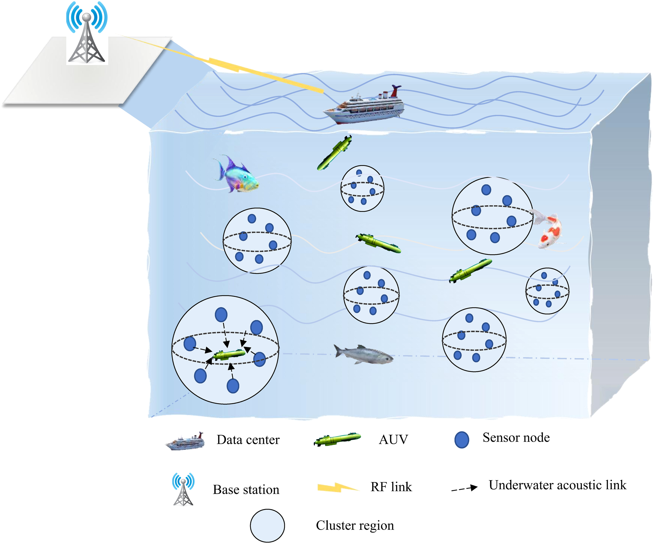
Figure 1. Multi-AUV-assisted data collection 3-D network model in UASNs.

To reduce the path length of the AUV, sensor nodes are clustered into groups. Traditionally, one sensor node is selected as the cluster head for each group to receive data from cluster members and forward the data to the AUV. However, this approach leads to the hotspot problem, i.e., the cluster head consumes energy at a faster rate. Though cluster head rotation methods can be applied to balance the energy consumption of sensor nodes, the energy consumed by secondary forwarding from cluster head to the AUV is unnecessary. In this paper, we choose a virtual cluster head for each cluster, which is a hovering point (HP) for the AUV rather than a real sensor node. During data collection, when the AUV reaches the HP, it acts as the cluster head and establishes acoustic communication links with sensor nodes in the cluster. In this way, the sensor nodes directly send data to the AUV, avoiding secondary forwarding. Suppose N sensor nodes are divided into M clusters. Meanwhile, there are M HPs $\mathscr{H}=\left\{h_1,h_2,\cdots ,h_M\right\}$. It should be noted that the value of M and the location of the HPs are not pre-known and are optimized by the proposed solution later. To guarantee that each AUV can visit at least one cluster, we have 1 ≤ K ≤ M. Table 1 and Table 2 present the notions and abbreviations used in this paper.

Table 1

Table 1. Notations summary.

Table 2

Table 2. Abbreviation table.

3.1 Underwater acoustic channel model

The underwater acoustic communication model applied in this work is described in Chaitanya et al. (2011) specifically. The path loss depends on communication distance d in km and carrier frequency f_c in kHz is expressed as Equation 1.

$\begin{array}{ll}A(d,f_c)=A_0{d}^{\zeta }a{(f_c)}^d& (1)\end{array}$

where A₀ is a normalized constant and ζ is the propagation loss coefficient. The value of ζ takes either 2 or 1 in spherical spreading and cylindrical spreading, respectively; generally, ζ = 1.5 in practical spreading. a(f_c) is the absorption coefficient, which can be expressed in dB/km as the function of f_c according to Thorp’s formula (Brekhovskikh et al., 2003), i.e., Equation 2:

$\begin{array}{ll}\begin{array}{ll}10\text{ log }a(f_c)\hfill & =\frac{0.11f_c^2}{1+f_c^2}+\frac{44f_c^2}{4100+f_c^2}+2.75\times {10}^{-4}{f}_c^2+0.003\hfill \end{array}& (2)\end{array}$

In addition, the path loss model of the acoustic channel can be expressed in dB as Equation 3:

$\begin{array}{ll}10\text{ log }A(d,f_c)=10\text{ log }{A}_0+\zeta 10\text{ log }d+d10\text{ log }a(f_c)& (3)\end{array}$

Ambient noise in underwater acoustic communication is determined by several factors, such as turbulence, the shipping activity in the surrounding region, the surface motion caused by wind-driven waves, and finally thermal noise. The constant surface motion due to wind-driven waves is a significant factor contributing to the noise at the operating frequencies of interest for underwater systems (100 Hz to 100 kHz). The noise can be modeled (Stojanovic, 2007):

$\begin{array}{ll}10\text{ log }{N}_t(f_c)=17-30\text{ log }{f}_c& \text{(4a)}\end{array}$

$\begin{array}{ll}\begin{array}{ll}10\text{ log }{N}_s(f_c)\hfill & =40+20(s-0.5)+26\text{ log }{f}_c-60\text{ log }(f_c+0.03)\hfill \end{array}& \text{(4b)}\end{array}$

$\begin{array}{ll}\begin{array}{ll}10\text{ log }{N}_w(f_c)\hfill & =50+7.5w^{1/2}+20\text{ log }{f}_c-40\text{ log }(f_c+0.4)\hfill \end{array}& \text{(4c)}\end{array}$

$\begin{array}{ll}10\text{ log }{N}_{th}(f_c)=-15+20\text{ log }{f}_c& \text{(4d)}\end{array}$

where N_t(f_c), N_s(f_c), N_w(f_c), and N_th(f_c) represent turbulence, shipping, waves, and thermal noise, and can be calculated by Equations 4a-4d, respectively. f_c is in kHz, s models the surface shipping activity ranging from 0 to 1, and w denotes the wind speed in m/s. The total acoustic channel noise consists of the four components, i.e., Equation 5:

$\begin{array}{ll}N(f_c)=N_t(f_c)+N_s(f_c)+N_w(f_c)+N_{th}(f_c)& (5)\end{array}$

Then, the normalized signal-to-noise ratio (SNR) at the receiver of the underwater acoustic communication link can be calculated as Equation 6 (Hollinger et al., 2011):

$\begin{array}{ll}\gamma (d,f_c)=\frac{1}{A(d,f_c)N(f_c)}& (6)\end{array}$

It can be seen that the SNR depends on the transmission distance under a fixed carrier frequency. Assuming additive white Gaussian noise (AWGN) channels, the capacity of the underwater acoustic channel between the AUV and sensor nodes can be given by Equation 7,

$\begin{array}{ll}R(d)=ℬ{\log }_2(1+{10}^{\frac{P_{tr}^{SL}}{10}}\gamma (d,f_c)/ℬ)& (7)\end{array}$

where $P_{tr}^{SL}$ is the source level of the transmitted signal in dB re µPa and ℬ is the communication bandwidth in Hz.

3.2 Energy consumption model

The energy consumption of the sensor node s_n is mainly caused by sending its data to the AUV. We assume that the transmitting power of sensor nodes is fixed; then, the energy consumption is dependent on the data transmission time. If the sensor node s_n is associated with h_m, the data transmission time of s_n is given by Equation 8:

$\begin{array}{ll}{\theta }_{m,n}=\frac{D_{n}L}{R(d_{m,n})}+\frac{d_{m,n}}{v_s}& (8)\end{array}$

where $D_n$ is the number of data packets that $s_n$ planned to upload to the AUV. $L$ is the packet length. $d_{m,n}={\Vert {\mathbf{\text{h}}}_m-{\mathbf{\text{q}}}_n\Vert }_2$ denotes the transmission distance between $h_m$ and $s_n$. $v_s$ is the sound speed. We use a matrix $\text{Γ}$ with binary variables ${\gamma }_{m,n}$ to indicate whether sensor node $s_n$ is associated with $h_m$. In particular, ${\gamma }_{m,n}=\left\{0,1\right\}$ with ${\gamma }_{m,n}=1$ meaning that $s_n$ belongs to the group of ${\mathbf{\text{h}}}_m$ and ${\gamma }_{m,n}=0$ otherwise. We can get the following constraints:

$\begin{array}{ll}{\gamma }_{m,n}=\{\begin{array}{cc}1,& d_{m,n}\le r_n^c\\ 0,& \text{otherwise}\end{array}& \text{(9a)}\end{array}$

$\begin{array}{ll}{\displaystyle \sum _{m=1}^M{\gamma }_{m,n}}=1,\forall n\in [1,N]& \text{(9b)}\end{array}$

$\begin{array}{ll}{\displaystyle \sum _{n=1}^N{\gamma }_{m,n}}\ge 1,\forall m\in [1,M]& \text{(9c)}\end{array}$

where $r_n^c$ is the communication range of sensor node s_n. Equation 9a indicates that the distance between the HP and its cluster members should be shorter than the communication range of sensor nodes. Equation 9b means that each sensor only associates with one HP and Equation 9c shows that each HP is associated with at least one sensor node. Through the above analysis, the energy consumed by sensor node s_n can be denoted by Equation 10:

$\begin{array}{ll}{E}_{s_n}={\displaystyle \sum _{m=1}^M{\gamma }_{m,n}{P}_{tr}^n{\theta }_{m,n}}& (10)\end{array}$

where $P_{tr}^n$ is the transmitting power of s_n. The total energy consumption of sensor nodes in S is represented as Equation 11:

$\begin{array}{ll}{E}_{\mathcal{S}}={\displaystyle \sum _{n=1}^N{E}_{s_n}}={\displaystyle \sum _{n=1}^N{\displaystyle \sum _{m=1}^M{\gamma }_{m,n}{P}_{tr}^n{\theta }_{m,n}}}& (11)\end{array}$

In addition, the energy consumption standard deviation σ_S is defined to measure the balance of sensor energy consumption in the network and can be calculated by Equation 12:

$\begin{array}{ll}{\sigma }_{\mathcal{S}}=\sqrt[2]{\frac{{\sum }_{n=1}^N{(E_{s_n}^{res}-{\overline{E}}_{\mathcal{S}}^{res})}^2}{N-1}}& (12)\end{array}$

where $E_{s_n}^{res}$ and ${\overline{E}}_{\mathcal{S}}^{res}$ represent the residual energy of sensor s_n and the average residual energy of N sensors in 𝒮 after data collection, respectively.

As for the AUVs, their energy consumption mainly includes the navigation energy and hovering energy. The communication energy consumption of AUVs can be neglected compared with motion energy (Hou et al., 2022). The hovering energy of AUVs can be denoted by Equation 13:

$\begin{array}{ll}{E}_{\mathcal{V}}^h={\displaystyle \sum _{n=1}^N{\displaystyle \sum _{m=1}^M{\gamma }_{m,n}{P}_a^h{\theta }_{m,n}}}& (13)\end{array}$

where $P_a^h$ is the hovering power of the AUV. The navigation time between ${\mathbf{\text{h}}}_i$ and ${\mathbf{\text{h}}}_j$ is ${\lambda }_{i,j}={\Vert {\mathbf{\text{h}}}_i-{\mathbf{\text{h}}}_j\Vert }_2/v_a,\forall i\ne j$, where $v_a$ is the navigation velocity of the AUV. From the AUV’s perspective, the network can be seen as a graph $\mathcal{G}=({\mathscr{H}}^{+},ℰ)$, where ${\mathscr{H}}^{+}=\mathscr{H}\cup s_0$, while $ℰ$ refers to the set of edges. We define a pathfinder matrix $X$, where ${[X]}_{ij}=x_{i,j}$ is the path indicator. $x_{i,j}=1$ means that the subpath ${\mathbf{\text{h}}}_i\to {\mathbf{\text{h}}}_j$ is traveled by the AUV; otherwise, $x_{i,j}=0$. Then, the navigation energy of the AUV can be formulated as Equation 14:

$\begin{array}{ll}{E}_{\mathcal{V}}^n={\displaystyle \sum _{i=0}^M{\displaystyle \sum _{j=0}^M{\lambda }_{i,j}{P}_a^n{x}_{i,j}}}& (14)\end{array}$

where $P_a^n$ is the propelling power of the AUV. The total energy of AUV is defined by Equation 15:

$\begin{array}{ll}{E}_{\mathcal{V}}=E_{\mathcal{V}}^n+E_{\mathcal{V}}^h={\displaystyle \sum _{n=1}^N{\displaystyle \sum _{m=1}^M{\gamma }_{m,n}{P}_a^h{\theta }_{m,n}}}+{\displaystyle \sum _{i=0}^M{\displaystyle \sum _{j=0}^M{\lambda }_{i,j}{P}_a^n{x}_{i,j}}}& (15)\end{array}$

3.3 Age of information model

The freshness of information is defined by the AoI. Let A_n(t) denote the instantaneous AoI of data retrieved from sensor s_n. We assume s_n adds timestamp $T_n^G$ to its packets. A_n(t) is shown as Equation 16:

$\begin{array}{ll}{A}_n(t)=\text{max }\{(t-t_n^G),0\},n=1,\cdots ,N.& (16)\end{array}$

In our scenario, AUVs offload the collected data to the data center for further analysis immediately when they return back to the data center. Thus, the AoI of data from s_n is determined by the sensor’s 226 uploading periods and AUV’s navigation periods. Let us take the sensor nodes visited by AUV $v_k$ as an example to derive the AoI. Suppose there are $M^k$ $\left({\displaystyle {\sum }_{k=1}^K{M}^k}=M\right)$ clusters assigned to AUV $v_k$ for data collection and vector ${\mathbf{\text{f}}}_k=[{\mathbf{h}}_{(0)}^k,{\mathbf{h}}_{(1)}^k,\cdots ,{\mathbf{h}}_{(M^k)}^k,{\mathbf{h}}_{(M^k+1)}^k]$ is used to denote the trajectory of $v_k$, where $h_{(0)}^k=h_{(M^k+1)}^k=s_0$. Meanwhile, ${\pi }_m=[s_{(1)}^m,\cdots ,s_{(\left|{\mathcal{J}}_m\right|)}^m]$ is defined to represent the uploading sequence vector of sensors, where ${\mathcal{J}}_m=\{s_n❘{\gamma }_{m,n}=1,s_n\in \mathcal{S}\}$ is the set of sensors that are associated with ${\mathbf{h}}_m$. If $s_n$ is associated with ${\mathbf{h}}_{(m)}^k$ and is scheduled to be the $j$th one to send its data, the AoI of data uploaded by $s_n$ when $v_k$ completes data collection at ${\mathbf{h}}_{(m)}^k$ can be represented as ${\displaystyle {\sum }_{i=j}^{\left|{\mathcal{J}}_{(m)}\right|}{\theta }_{(m),(i)}}$. We also label the AoI of $s_n$ as $A_{(m),(j)}^k$ and its final expression when $v_k$ arrives at $s_0$ is shown as Equation 17:

$\begin{array}{ll}{A}_{(m),(j)}^k={\displaystyle \sum _{i=j}^{\left|{\mathcal{J}}_{(}m)\right|}{\theta }_{(m),(i)}}+{\displaystyle \sum _{i=m}^{M^k}{\lambda }_{(i),(i+1)}}+{\displaystyle \sum _{l=m+1}^{M^k}{\displaystyle \sum _{i=1}^{\left|{\mathcal{J}}_{(l)}\right|}{\theta }_{(l),(i)}}}& (17)\end{array}$

where the second and third terms are the navigation time and the uploading time of all the clusters after v_k leaves h_m. Thus, the sum AoI of sensors collected by v_k can be expressed as Equation 18:

$\begin{array}{ll}\begin{array}{l}{A}^k={\displaystyle \sum _{m=1}^{M^k}{\displaystyle \sum _{j=1}^{\left|{\mathcal{J}}_{(m)}\right|}{A}_{(m),(j)}^{(k)}}}\\ ={\displaystyle \sum _{m=1}^{M^k}{\displaystyle \sum _{j=1}^{\left|{\mathcal{J}}_{(m)}\right|}\left({\displaystyle \sum _{l=m+1}^{M^k}{\displaystyle \sum _{i=1}^{\left|{\mathcal{J}}_{(l)}\right|}{\theta }_{(l),(i)}}+{\displaystyle \sum _{i=j}^{\left|{\mathcal{J}}_{(m)}\right|}{\theta }_{(m),(i)}}+{\displaystyle \sum _{i=m}^{M^k}{\lambda }_{(i),(i+1)}}}\right)}}\\ ={\displaystyle \sum _{m=1}^{M^k}{\displaystyle \sum _{j=1}^{\left|{\mathcal{J}}_{(m)}\right|}\left({\displaystyle \sum _{i=m}^{M^k}{\lambda }_{(i),(i+1)}}+{\displaystyle \sum _{l=m}^{M^k}{\displaystyle \sum _{i=1}^{\left|{\mathcal{J}}_{(m)}\right|}{\theta }_{(l),(i)}}-{\displaystyle \sum _{i=1}^{j-1}{\theta }_{(m),(i)}}}\right)}}\end{array}& (18)\end{array}$

By recursive computation, it can be further derived as follows.

PROPOSITION 1. The sum AoI of all sensors collected by AUV v_k can be expressed as Equation 19 (Liu et al., 2020b):

$\begin{array}{ll}\begin{array}{ll}{A}^k\hfill & ={\displaystyle \sum _{m=2}^{M^k}{\xi }^{(m-1)}{\psi }^{(m)}+{\displaystyle \sum _{i=1}^{M^k}{\xi }^i{\lambda }_{(i),(i+1)}}+{\displaystyle \sum _{m=1}^{M^k}{\displaystyle \sum _{j=1}^{\left|{\mathcal{J}}_{(m)}\right|}j{\theta }_{(m),(j)}}}}\hfill \end{array}& (19)\end{array}$

where ${\xi }^{(m)}={\displaystyle {\sum }_{i=1}^m\left|{\mathcal{J}}_{(i)}\right|}$ is the number of sensors visited from the first cluster to the mth cluster in the trajectory of $v_k$ and ${\psi }^{(m)}={\displaystyle {\sum }_{j=1}^{\left|{\mathcal{J}}_{(m)}\right|}{\theta }_{(m),(j)}}$ denotes the total amount of uploading time of the sensors in the mth cluster visited by v_k.

PROOF. The details of the proof are provided in Appendix 1.

For all the sensors in 𝒮, their average AoI can be formulated as Equation 20:

$\begin{array}{ll}\overline{A}=\frac{1}{N}{\displaystyle \sum _{k=1}^K{A}^k}& (20)\end{array}$

Observing Equation 19, we can easily find that the average AoI is jointly determined by the clustering results of sensors, the navigation trajectory of AUVs, and the uploading sequence of sensors.

3.4 Problem formulation and analysis

In this work, both the energy consumption and the average AoI are considered. The objective is to minimize the total energy consumption of the whole network while simultaneously minimizing the average AoI $\stackrel{-}{A}$ as follows:

$\begin{array}{ll}(\text{P}1):\underset{M,\mathscr{H},\mathbf{\text{Γ}},\mathbf{X}}{\min }{E}_{\mathcal{V}}+E_{\mathcal{S}}& \text{(21a)}\end{array}$

$\begin{array}{ll}\underset{M,\mathscr{H},\mathbf{\text{Γ}},\mathbf{X},{\mathbf{f}}_k,{\pi }_m}{\min }\overline{A}& \text{(21b)}\end{array}$

$\begin{array}{ll}s.t.1\le K\le M& \text{(21c)}\end{array}$

$\begin{array}{ll}{E}_{s_n}\le E_{s_n}^{ini}& \text{(21d)}\end{array}$

$\begin{array}{ll}{\displaystyle \sum _{i=1}^{M^k}{P}_a^n{\lambda }_{(i),(i+1)}}+{\displaystyle \sum _{m=1}^{M^k}{\displaystyle \sum _{i=1}^{\left|{\mathcal{J}}_{(m)}\right|}{\theta }_{(m),(i)}{P}_a^h\le E_a^{ini}}}& \text{(21e)}\end{array}$

$\begin{array}{ll}{\displaystyle \sum _{j=1}^M{x}_{0,j}}={\displaystyle \sum _{i=1}^M{x}_{i,0}}=K& \text{(21f)}\end{array}$

$\begin{array}{ll}{\displaystyle \sum _{i=0}^M{x}_{i,j}}={\displaystyle \sum _{j=0}^M{x}_{i,j}}=1,\forall i,j=1,\dots ,M& \text{(21g)}\end{array}$

$\begin{array}{ll}{\displaystyle \sum _{m=1}^M{\gamma }_{m,n}}=1,\forall n=1,\dots ,N& \text{(21h)}\end{array}$

$\begin{array}{ll}{\displaystyle \sum _{n=1}^N{\gamma }_{m,n}}\ge 1,\forall m=1,\cdots ,M& \text{(21i)}\end{array}$

$\begin{array}{ll}{x}_{i,j},{\gamma }_{m,n}\in \left\{0,1\right\}& \text{(21j)}\end{array}$

where $E_{s_n}^{ini}$ and $E_a^{ini}$ are the initial energy of each sensor and AUV, respectively. Equation 21c indicates that the number of clusters should be less than that of AUVs. Equations 21d and 21e impose the energy constraints of sensor nodes and AUVs. Equation 21f means that all the AUVs are released from the data center and then return back after completing data collection tasks. Equation 21g reflects that each sensor is visited only once. The meaning of Equations 21h, 21i and 21j has been demonstrated in Section 3.2. Obviously, Equation 21 is a MILP problem, which is NP-hard.

Observing the expression of the optimization functions, E_𝒮 is determined by the association γ_m,n and the position of h_m. Besides the above factors, E_𝒱 is also affected by the path of AUVs. $\stackrel{-}{A}$ is determined by the data uploading time, the navigation time of AUV, the number of sensors in each cluster, and the uploading sequence of sensors. The uploading time of s_n is influenced by the association γ_m,n and the location of h_m. Thus, we can find that the optimization problem is determined jointly by the clustering result, the location of HPs, the navigation path of AUVs, and the uploading sequence of sensors in each cluster.

4 Proposed scheme

In this section, we propose a two-stage solution to solve the optimization problem formulated in Equation 21a. First, we design a cluster-based AUV scheduling data transmission protocol to optimize the clustering result, the locations of HPs, and the transmission sequence of sensors in each cluster. Then, considering the complexity of the problem, we propose a combinatorial heuristic algorithm to perform cluster allocation and path planning for AUVs. Based on the transmission protocol and path planning, the AoI and energy consumption in multi-AUV-assisted data collection are jointly optimized.

4.1 Cluster-based AUV scheduling data transmission protocol

In general, sensor nodes are deployed randomly to imitate the practical scenario in UASNs. To reduce the path length of AUVs, sensor nodes are divided into groups so that AUVs can visit each group to collect data efficiently. Kmeans clustering is the ideal method for clustering groups. However, two problems often arise in the practical application of the Kmeans algorithm. The first issue is that the Kmeans clustering algorithm requires the number of clusters as an input parameter, which is not easily known in advance. The second issue is that initial clustering centers must be selected before Kmeans clustering. These two parameters affect the final clustering results. In UASNs, the coordinates of the sensors are available, but the number of clusters and the initial clustering centers are difficult to estimate. In order to solve this problem, we adopt the Canopy algorithm as a preliminary step to the Kmeans clustering algorithm. The Canopy algorithm is a rough clustering method, which only requires the coordinates of sensor nodes as input and outputs the number of clusters and cluster centers. Nevertheless, the clustering result of the Canopy algorithm is with low accuracy. To this end, we use the number of clusters and cluster centers from the Canopy algorithm as input parameters to the Kmeans algorithm to obtain the final clustering results. We call the proposed algorithm as the CK clustering algorithm, which combines the advantages of Canopy and Kmeans algorithms. The details of the CK clustering algorithm are shown below.

The Canopy algorithm is an unsupervised pre-clustering algorithm. As shown in Figure 2, for the given sensor set 𝒮, the Canopy algorithm sets two area radius thresholds Z₁ and Z₂, where (Z₁ > Z₂). Then, a sensor s_i is randomly selected as the first canopy center. Next, the sensor that is set as center would be removed from S, i.e., 𝒮^′ = 𝒮\s_i. For each sensor in S^′, calculate the distance between it and the current canopy center. There are three possible cases. If the distance is less than Z₂, the sensor is considered to be a member of the corresponding canopy and cannot belong to another canopy. Afterwards, the sensor will be removed from 𝒮^′ to avoid adding to another canopy. If the distance is greater than Z₁, the sensor is regarded as a new canopy center and removed from 𝒮^′. If the distance is greater than Z₂ and less than Z₁, the sensor is kept in S^′ to participate in the next round of clustering process. The above process should be repeated until the dataset reaches empty.

Figure 2

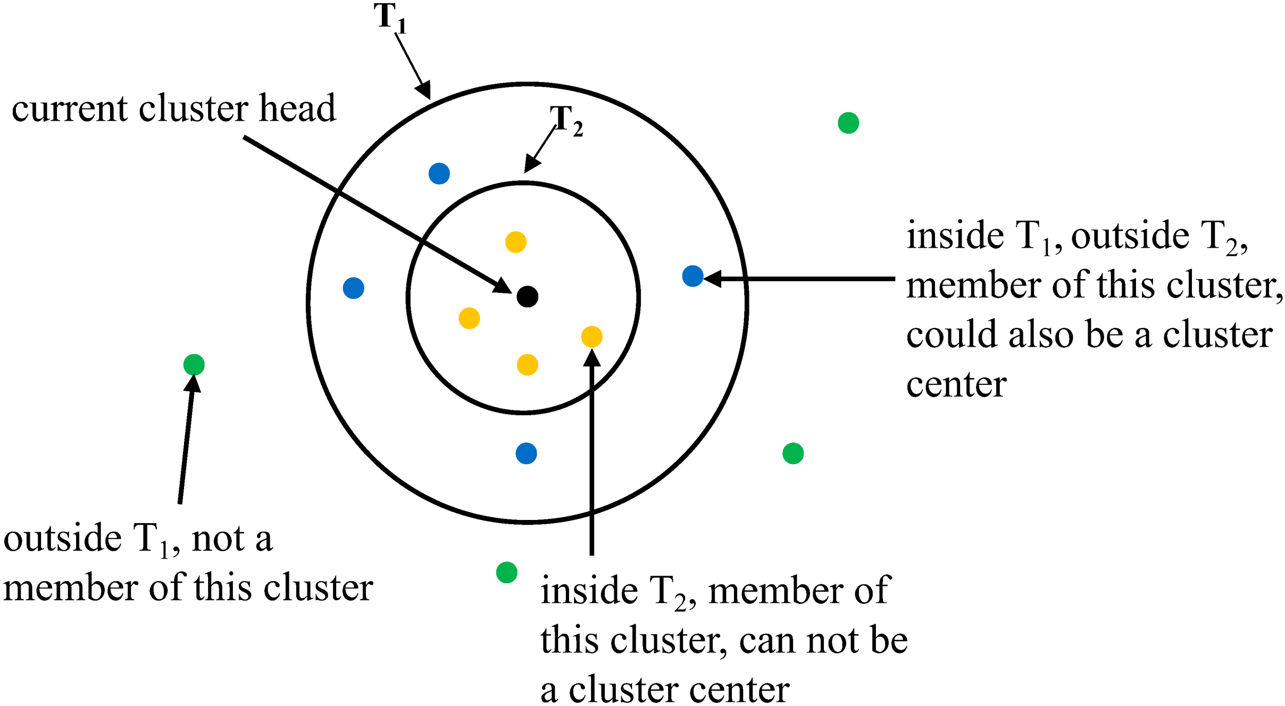
Figure 2. Process of canopy clustering.

Through the Canopy algorithm, we can get the number of canopies and their centers. For the sake of precise clustering, the result of the Canopy algorithm is used as input to Kmeans algorithm. The canopy centers are selected as initial cluster centers of Kmeans algorithm. Then, calculate the distance between the remaining sensor nodes with each initial cluster center. The sensor nodes will be associated with the nearest cluster center. After completing the association of all sensor nodes with cluster centers, the cluster centers are updated according to Equation 22:

$\begin{array}{ll}{C}_i{}^{\prime }=\frac{1}{\left|S_i\right|}{\displaystyle \sum _{{\mathbf{q}}_n^s\in S_i}{\mathbf{q}}_n^s}& (22)\end{array}$

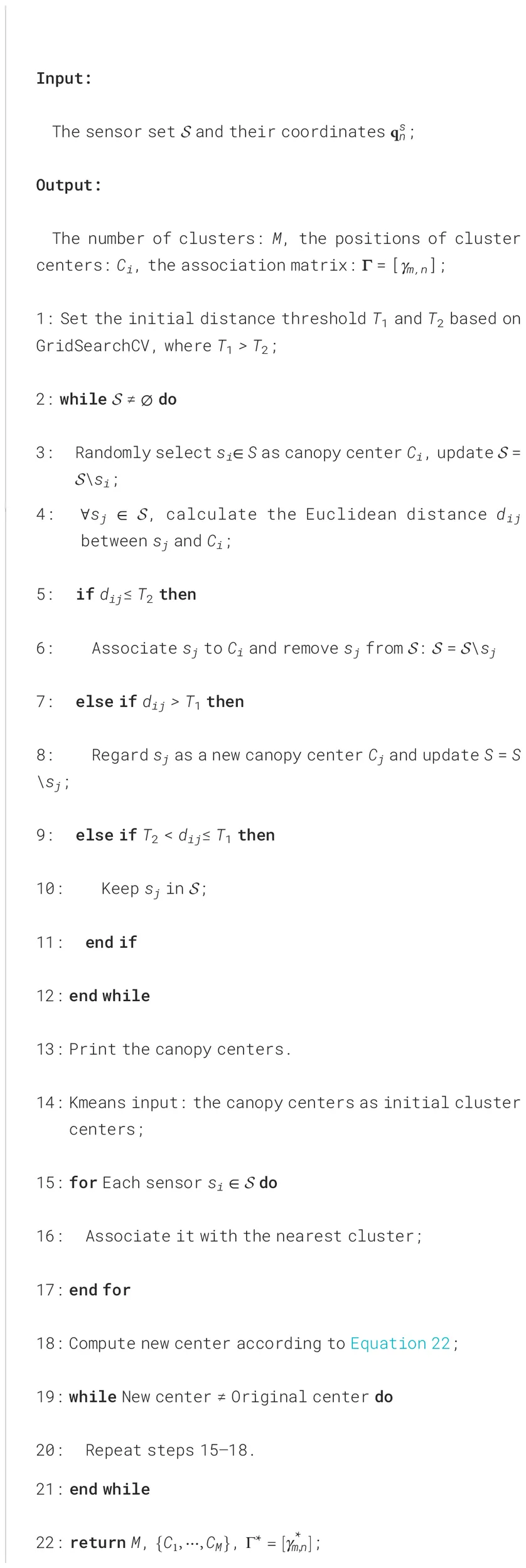
where ${C^{\prime }}_i$ is the new center of cluster $S_{i·}\left|S_i\right|$ and ${\mathbf{q}}_n^s$ denote the number of sensors in S_i and the coordinates of s_n, respectively. For each cluster S_i, we check whether ${C^{\prime }}_i$ is equal to C_i, where C_i is the clustering center from the last computation. If all the cluster centers remain unchanged, the clustering process should be stopped and output the Kmeans clustering results, i.e., the location of the cluster centers and the association between the sensor nodes and the cluster centers. Otherwise, the steps of dividing clusters and updating the clustering centers would be performed cyclically. The specific steps of the CK clustering algorithm are depicted in Algorithm 1. The Canopy algorithm determines the number of canopies and the initial centers from lines 1 to 13. Kmeans algorithm performs precise clustering from lines 15 to 21.

Algorithm 1. The CK clustering algorithm.

In previous works (Han et al., 2021; Omeke et al., 2021), the sensor node closest to the cluster center is appointed as the cluster head, which is responsible for gathering the data from the cluster members and forwarding it. However, as we have stated in Section 3, this approach introduces the problem of unbalanced energy consumption and unnecessary secondary forwarding. In this paper, we directly select the cluster center as the virtual cluster head of the cluster, which is not a sensor entity. The virtual cluster head is a hovering position reserved for the AUV, i.e., h_m = C_m. When the AUV arrives at h_m, it establishes communication links with the sensor nodes in the cluster to collect data. Through CK clustering and virtual cluster head selection, we associate each sensor node with the nearest hover point.

To collect data efficiently, we design a scheduling-based data transmission protocol. For simplicity, we take the data transmission process in one cluster as an example to illustrate the protocol, which is shown in Figure 3. Upon hovering at h_m, the AUV immediately sends an ANNUNCIATION packet (AnP) to wake up cluster members. Since the locations of cluster members are known, the propagation delay can be easily computed. AnP contains the AUV’s ID and the propagation delays from the AUV to each cluster member. Note that the propagation delay has an impact on determining when the sensor should send its REQUEST packet (ReP) and DATA packet (DaP). After the AnP is transmitted, the AUV starts a timeout $T_{ReP}^{TO}$ to wait for replies from sensors. Ideally, the ReP from sensors that are associated with h_m should arrive at the AUV before $T_{ReP}^{TO}$ expires. The rule of thumb is that the sensor responds ReP immediately upon receiving the AnP. However, ReP collisions occur occasionally, which reduces the channel utilization and throughput. Fortunately, propagation delays included in AnP can be used to avoid ReP collisions. First, the sensor ranks the propagation delays in ascending order. Suppose that the sensor finds itself with order l, the time at which it should send its own ReP can be calculated as:

Figure 3

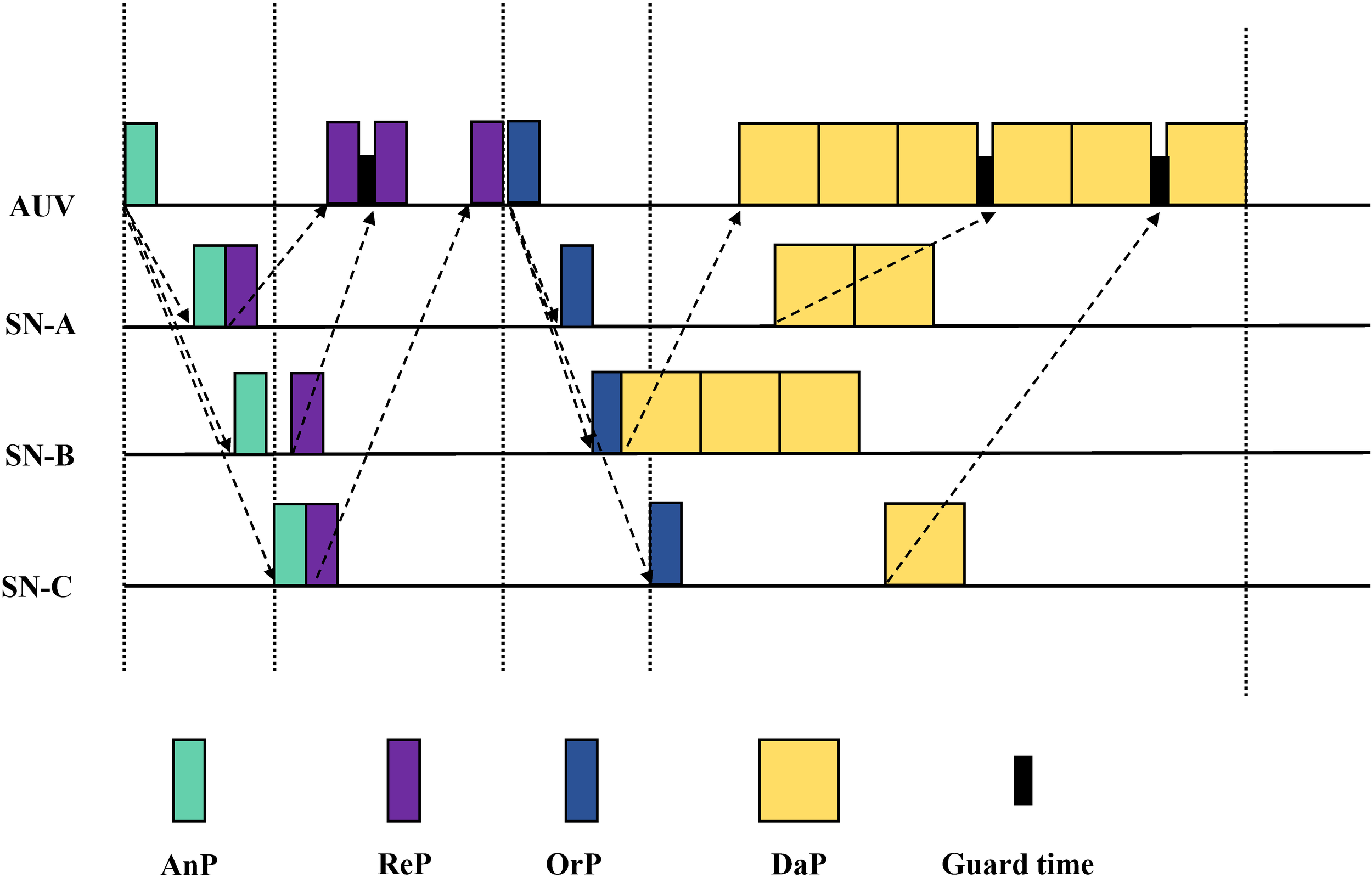
Figure 3. Data transmission protocol.

$\begin{array}{ll}\begin{array}{ll}{t}_{(l)}^{ReP}=\text{max }\{\hfill & t_{(l)}^{AnP},t_{(l-1)}^{ReP}+d_{m,(l-1)}/v_s+T_g+T_{ReP}-d_{m,(l)}/v_s\}\hfill \end{array}& (23)\end{array}$

where $t_{(l)}^{AnP}$ is the time at which the sensor receives the $AnP$, $d_{m,(l-1)}$ is the propagation delay between AUV and the sensor with order $l-1$, $T_g$ is a small guard time, and $T_{ReP}$ is the packet duration of $ReP$. In Equation 23, $t_{(l-1)}^{ReP}$ is involved in the calculation of $t_{(l)}^{ReP}$. The $t_{(l)}^{ReP}$ can be easily calculated step by step when $t_{(1)}^{ReP}$ is known. Since the $AnP$ is sent from the AUV at the same time, $t_{(1)}^{ReP}$ can be calculated as Equation 24:

$\begin{array}{ll}{t}_{(1)}^{ReP}=t_{(1)}^{AnP}=t_{(l)}^{AnP}-d_{m,(l)}/v_s+d_{m,(1)}/v_s& (24)\end{array}$

From the perspective of AUV, the length of $T_{ReP}^{AUV}$ needs to cover from sending $AnP$ to the arrival of the last $ReP$. For the sensor with order $\left|{\mathcal{J}}_m\right|$, the maximum back-off interval could be $(\left|{\mathcal{J}}_m\right|-1)(T_g+T_{ReP})$. Thus, the expression of $T_{ReP}^{TO}$ is $2d_{m,(\left|{\mathcal{J}}_m\right|)}/v_s+(\left|{\mathcal{J}}_m\right|-1)(T_g+T_{ReP})$.

The number of data packets (i.e., D_n) that sensor s_n plans to transmit and its own ID should be included in the ReP. After sending the ReP, s_n starts a timeout $T_{OrP}^{TO}$ within which it expects to receive an ORDER packet (OrP) from the AUV. Naturally, for the sensor with order l, its $T_{OrP}^{TO}$ can be calculated as $t_{\left|{\mathcal{J}}_m\right|}^{ReP}-t_l^{ReP}+T_{ReP}+2d_{m,(\left|{\mathcal{J}}_m\right|)}$. As we have analyzed, uploading the sequence of sensor nodes influences the AoI. When $T_{OrP}^{TO}$ expires, the AUV is supposed to determine the uploading sequence and transmission time for all sensor nodes in the cluster. Based on the D_n extracted from the received RePs, the AUV can calculate the sensor’s uploading time θ_m,n according to Equation 8. We find that the descending order of θ_m,n is the optimal uploading sequence. Specifically, for any given navigation trajectory f_k and association matrix Γ, the first and second items of Equation 19 are fixed. The AoI is solely determined by the third item ${\displaystyle {\sum }_{m=1}^{M^k}{\displaystyle {\sum }_{j=1}^{\left|{\mathcal{J}}_{(m)}\right|}j{\theta }_{(m),(j)}}}$, which depends on the sensor’s uploading sequence in each cluster. Giving higher uploading priority to sensor nodes with greater uploading time can minimize the third term, i.e., Equation 25:

$\begin{array}{ll}{\theta }_{(m),(1)}\ge {\theta }_{(m),(2)}\ge \cdots \ge {\theta }_{(m),(\left|{\mathcal{J}}_{(m)}\right|)}& (25)\end{array}$

It can be proved by the law of contradiction. We assume that the uploading sequence is not in the descending order of uploading time, then it certainly satisfies $\exists j>i,{\theta }_{m,(j)}\ge {\theta }_{m,(i)}$. Thus, $j({\theta }_{m,(j)}-{\theta }_{m,(i)})\ge i({\theta }_{m,(j)}-{\theta }_{m,(i)})$, then shift the terms to get $i{\theta }_{m,(i)}+j{\theta }_{m,(j)}\ge i{\theta }_{m,(j)}+j{\theta }_{m,(i)}$, which contradicts our goal of minimizing ${\sum }_{m=1}^{M^k}{\sum }_{j=1}^{\left|{\mathcal{J}}_{(m)}\right|}j{\theta }_{(m),(j)}$. The result can be easily extended to all the non-descending sequences. Obviously, when the sensors in each cluster upload data in the descending order of their uploading time, the value of ${\displaystyle {\sum }_{m=1}^{M^k}{\displaystyle {\sum }_{j=1}^{\left|{\mathcal{J}}_{(m)}\right|}j{\theta }_{(m),(j)}}}$ gets minimum.

With the determination of uploading sequence, the AUV can calculate when the sensor should start transmitting its DaP. In this article, we compute the scheduling time for each sensor, which refers to the expected time interval from receiving the OrP to the start of DaP transmission. For the ith sensor, its scheduling time $t_i^{sch}$ is denoted as Equation 26.

$\begin{array}{ll}{t}_{(i)}^{sch}=\{\begin{array}{cc}0,& i=1\\ d_{m,(1)}/v_s+(d_{m,(1)}/v_s+{\theta }_{(m),(1)}+T_g)-d_{m,(2)}/v_s,& i=2\\ t_{i-1}^{sch}+d_{m,(i-1)}/v_s+{\theta }_{(m),(i-1)}+T_g-d_{m,(i)}/v_s,& 3\le i\le \left|{\mathcal{J}}_m\right|\end{array}& (26)\end{array}$

Then, the scheduling time is embedded into the OrP and sent to the sensors. After that, the AUV starts a timeout $T_{DaP}^{TO}$ to receive DaPs. The expression for $T_{DaP}^{TO}$ is shown as Equation 27:

$\begin{array}{ll}{T}_{DaP}^{TO}=t_{({\mathcal{J}}_m)}^{sch}+{\theta }_{m,({\mathcal{J}}_m)}+d_{m,(\left|{\mathcal{J}}_m\right|)}/v_s+T_g& (27)\end{array}$

If the sensor receives the OrP before $T_{OrP}^{TO}$ expires and finds its ID in the packet, it stops $T_{OrP}^{TO}$ and starts $t_{(i)}^{sch}$. Otherwise, it returns to an IDLE state and waits for another AnP. When $t_{(i)}^{sch}$ expires, the sensor transmits DaP to the AUV. All the DaPs will form a packet train at the AUV. Through the cluster-based AUV scheduling data transmission protocol, the AUV accomplishes data collection from sensors within a cluster.

4.2 PGS-based AUV trajectory planning

Based on the CK-clustering and scheduling protocol above, the association between the HPs and the sensor nodes, the location of HPs, and the uploading sequence of the sensor nodes in each cluster are determined. In Equations 21a and 21b, the items related to these variables are also determined. Specifically, they are the E_𝒮, the first item of E_𝒱. In addition, the first and the third items of $\overline{A}$ are included. The second item of E_𝒱, i.e., ${\displaystyle {\sum }_{i=0}^M{\displaystyle {\sum }_{j=0}^M{\lambda }_{i,j}{P}_a^n{x}_{i,j}}}$, and the second item of $\overline{A}$, i.e., ${\displaystyle {\sum }_{k=1}^K{\displaystyle {\sum }_{i=1}^{M^k}{\xi }^i{\lambda }_{(i),(i+1)}}}$ could be further optimized. The objective of the subproblem is modeled as Equation 28:

$\begin{array}{ll}\begin{array}{l}(P2):\underset{\mathbf{X}}{\min }\sum _{i=0}^M\sum _{j=0}^M{\lambda }_{i,j}{P}_a^n{x}_{ij}\\ \underset{\mathbf{X},{\mathbf{f}}_k}{\min }\sum _{k=1}^K\sum _{i=1}^{M^k}{\xi }^i{\lambda }_{(i),(i+1)}\\ s.t.(22\text{c}),(22\text{e}),(22\text{f}),(22\text{g}),x_{ij}\in \left\{0,1\right\}.\end{array}& (28)\end{array}$

Both objective functions are only affected by the AUVs’ trajectories. Moreover, the pathfinder matrix X is decided by the trajectory of each AUV, i.e., [f₁,f₂,···,f_K]. Then, the next step is to plan trajectories for the K AUVs to traverse all the HPs. The problem (P2) can be reformulated as a special multi-AUV traveling salesman problem (MTSP):

$\begin{array}{ll}\begin{array}{l}(P3):\underset{\left\{{\mathbf{f}}_1,{\mathbf{f}}_2,\cdots ,{\mathbf{f}}_K\right\}}{\text{min}}\sum _{k=1}^K\sum _{i=1}^{M^k}({\xi }^i+P_a^n){\lambda }_{(i),(i+1)}\\ s.t.(22\text{c}),(22\text{e}),(22\text{f}),(22\text{g}).\end{array}& (29)\end{array}$

MTSP is NP-hard. In order to reduce the computational complexity, we propose a combinatorial heuristic algorithm to solve this problem. The algorithm is named PGS, which combines the advantages of particle swarm optimization (PSO) algorithm, genetic algorithm (GA), and simulated annealing (SA) algorithm. On the one hand, considering the characteristics of the problem, we apply the particles updating method of discrete PSO and the crossover and mutation operation of GA to PGS (Roberge et al., 2012; Abhishek et al., 2020). On the other hand, PGS retains the strategies of particle information exchange and collaboration in PSO and introduces the annealing operation to enhance the global optimization ability of particles (Lin et al., 2023).

The goal of P3 is to find a path ${\mathbf{f}}_k=[{\mathbf{h}}_{(0)}^k,{\mathbf{h}}_{(1)}^k,\cdots ,{\mathbf{h}}_{(M^k)}^k,h_{(M^k+1)}^k]$ for AUV $v_k,(k=1,\cdots ,K)$ while minimizing Equation 29. We adopt the integer sequence as the path encoding in PGS. For example, path $2\to 5\to 4\to 3\to 1\to 0$ can be expressed as [0, 2, 5, 4, 3, 1, 0]. Since the initial solution has a significant impact on the quality of the final solution in the heuristic algorithm, we apply the light ray optimization (LRO) algorithm to obtain high-quality initial solutions. We first introduce several concepts: (1) Current HP’s density: the shortest path from the current HP to another HP that has not been visited; (2) Frontier HP’s density: the average path length among the remaining HPs except the HPs that have been visited; (3) Reflection: an unvisited HP is randomly selected as the next one; and (4) Refraction: select the unvisited HP with the shortest distance from the current HP as the next one. The procedure of LRO to produce the initial solution is as follows: (1) Randomly select an HP as the first visited one and calculate the current HP’s density and the frontier HP’s density respectively; (2) Compare them; if the current HP density is greater than the frontier HP density, perform reflection; otherwise, perform refraction; (3) Repeat the second step until every HP is included in the trajectory; and (4) Let each HP serve as the first visited point and repeat the above three steps to obtain M initial solutions.

In the classic PSO algorithm, the particles update themselves by inheriting the speed of the previous moment, self-learning, and information interaction of the population, which is shown as:

$\begin{array}{ll}\begin{array}{ll}{\nu }_i^{k+1}\hfill & =\omega {\nu }_i^k+c_1{r}_1({\text{p}}_{i,best}^k-{\text{z}}_i^k)+c_2{r}_2({\text{G}}_{best}^k-{\text{z}}_i^k)\hfill \\ {\text{z}}_i^{k+1}\hfill & ={\text{z}}_i^k+{\nu }_i^{k+1}\hfill \end{array}& (30)\end{array}$

where $z_i^k$represents the position of particle i at time $k,{\nu }_i^k$ denotes the velocity of particle i at time k. $p_{i,best}^k$p refers to the local optimal solution searched by particle i at time $k,G_{best}^k$ refers to the global optimal solution searched by the whole population at time k. ω is the inertia factor. c₁ and c₂ are the local learning factor and global learning factor, which represent the ability to learn from their own experience and population experience, respectively. r₁ and r₂ are random numbers in [0,1], increasing the randomness of the searching process. However, Equation 30 is designed for continuous domain and cannot be applied to discrete problems. For the proposed problem P3, we combine the crossover and mutation operations with the particles’ dating mode of PSO to achieve optimization searching in discrete problems:

$\begin{array}{ll}\begin{array}{ll}{\nu }_i^{k+1}\hfill & =\omega \odot {\nu }_i^k\oplus r_1({\text{p}}_{i,best}^k\otimes {\text{z}}_i^k)\oplus r_2({\text{g}}_{best}^k\otimes {\text{z}}_i^k)\hfill \\ {\text{z}}_i^{k+1}\hfill & ={\text{z}}_i^k\oplus {\nu }_i^{k+1}\hfill \end{array}& (31)\end{array}$

where ⊗ and ⊙ denote the crossover and mutation operations, respectively. ⊕ represents accumulation of operations performed on particles. The item ω ⊙ ${\nu }_i^k$ indicates that the mutation operation occurs with probability ω. The items $r_1({\text{p}}_{i,best}^k\otimes {\text{z}}_i^k)$ and $r_2({\text{g}}_{best}^k\otimes {\text{z}}_i^k)$ indicate that the outcomes resulting from the crossover operation of particle i with ${\text{p}}_{i,best}^k$ and ${\text{g}}_{best}^k$ will be adopted with probabilities r₁ and r₂, respectively.

In the PSO algorithm, most of the particles tend to gather near the local optimal area when the current optimal positions of particles approach the local optimal solution, i.e., falling into local optimum. In order to strengthen the global search ability of particles and augment the probability of escaping from local optimum, the annealing method in the SA algorithm is introduced. The Metropolis sampling criterion is the core idea of annealing, which is used to calculate the probability that the new solution can be accepted:

$\begin{array}{ll}{P}_{i\to j}=\{\begin{array}{l}1,\hspace{1em}{E}_j<E_i,\hfill \\ \text{exp }\left(-\frac{E_j-E_i}{T}\right),E_j\ge E_i.\hfill \end{array}& (32)\end{array}$

where E_i and E_j are the energy of the particles in state i and j, respectively. T represents the current temperature. P_i→j denotes the probability of the system state transferring from state i to state j. In the PGS, we define the fitness function as $f={\displaystyle {\sum }_{k=1}^K{\displaystyle {\sum }_{i=1}^{M^k}({\xi }^i+P_n^a){\lambda }_{(i),(i+1)}}}$. Referring to Equation 32, the probability of the new solution being accepted is:

$\begin{array}{ll}P=\{\begin{array}{l}1,\hspace{1em}f({\text{z}}_i^{k+1})<f({\text{z}}_i^k)\hfill \\ \text{exp }\left(-\frac{f(z_i^{k+1})-f(z_i^k}{T}\right),f({\text{z}}_i^{k+1})\ge f({\text{z}}_i^k)\hfill \end{array}& (33)\end{array}$

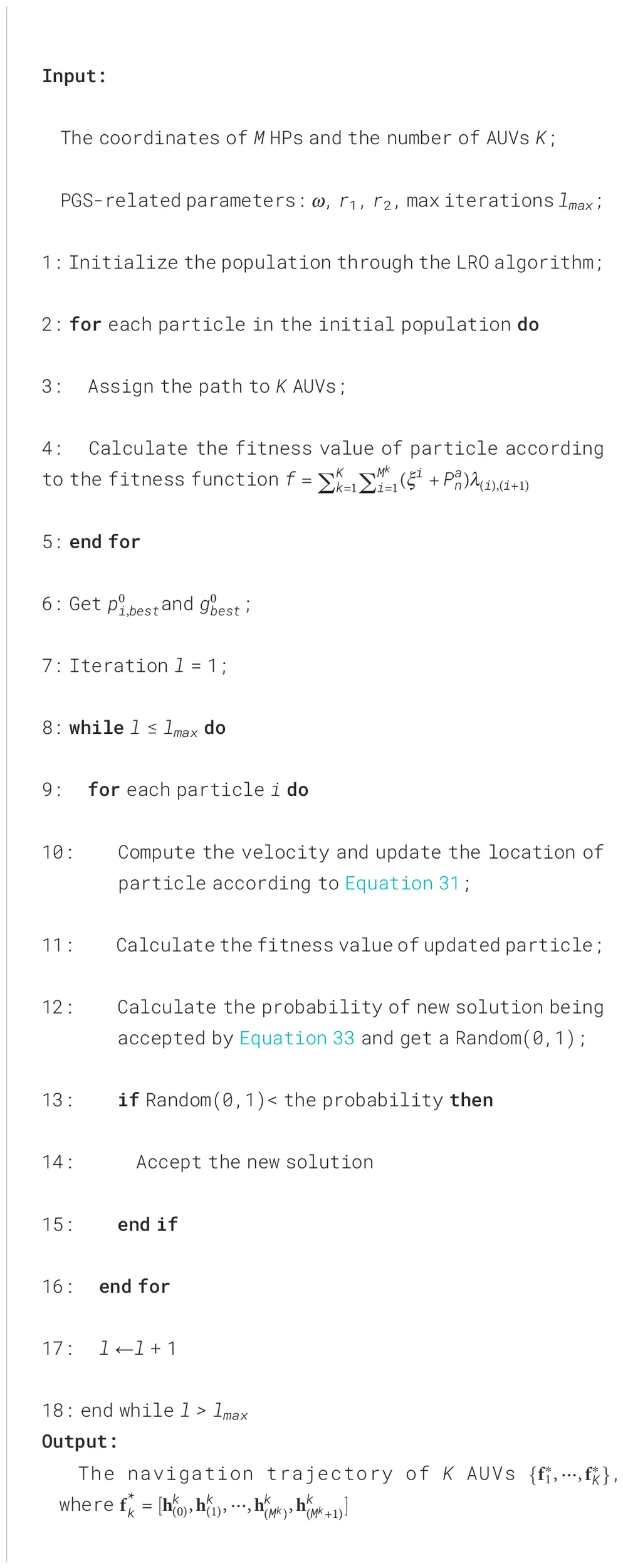
The details of the proposed PGS algorithm are shown in Algorithm 2.

Algorithm 2. PGS algorithm.

4.3 MADCS design

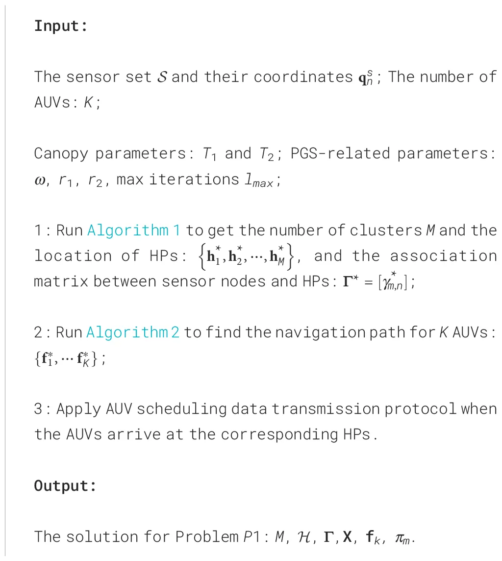
Based on the above solutions, we propose a MADCS to solve the P1, an AoI and energy joint optimization problem. The procedure of MADCS is shown in Algorithm 3 and the main steps of MADCS are as follows. First, we construct the cluster-based network by Algorithm 1 to determine associations between sensor nodes and HPs, and then find the position of HPs. In the second phase, we plan the navigation path for each AUV via Algorithm 2 according to the different numbers of AUVs. Upon arriving at HPs, the AUV starts the scheduling protocol described in Section 4.1 to complete data transmission. After traversing the HPs assigned to it, the AUV returns to the surface data center to offload all the collected data.

Algorithm 3. MADCS.

5 Simulation results and analysis

5.1 Simulation setup

In this section, extensive simulations are carried out to evaluate the performance of the proposed MADCS algorithm. We first introduce the scenario setup of simulations. Consider an AUV-assisted UASN that consists of a data center, M AUVs, and N sensor nodes. The value of N is set to 150 unless otherwise specified. The sensor nodes are randomly deployed in a 3D underwater environment with a size of 5,000 m × 5,000 m × 1,000 m. The data center is located at the sea surface with coordinate (0, 0, 1,000). All AUVs start from the data center and return back after traversing the assigned HPs. The parameters of underwater acoustic modems are chosen from technical specifications of the EvoLogics S2C modems (Favaro et al., 2013; EvoLogics, 2023). The transmission power is set to 154 dB re µPa², which yields a transmission range of approximately 1,000 m. The carrier frequency and the bandwidth of the PHY layer are 26 and 16 kHz, respectively. Other detailed parameters are listed in Table 3.

Table 3

Table 3. Simulation parameters.

5.2 Analysis of hyper-parameters in clustering

In simulations, the CK algorithm is firstly used to obtain the association matrix between the sensor nodes and the HPs, and the positions of HPs. T₁ and T₂ are two important hyper-parameters in clustering and have a great impact on the clustering results. On the one hand, if T₁ is too large, it will result in a high overlap of canopies, where one node belongs to multiple canopies. On the other hand, if T₂ is excessively large, it will lead to a low number of canopies. Conversely, when T₂ is too small, the number of canopies increases, leading to an increase in computational time. In this paper, we adopted the GridSearchCV method to choose the values of T₁ and T₂. The mean distance of node pairs among $\mathcal{S}$ is denoted as $\overline{d}=\frac{1}{N(N-1)}{\displaystyle {\sum }_{i,j=1}^{N}d(s_i,s_j)}$. The minimum distance between nodes in the $\mathcal{S}$ is denoted as $d_{min}=\text{min }\{d(s_i,s_j)❘i\ne j\}$. We set the grid search range of $T_1$ and $T_2$ are $[\frac{\overline{d}+d_{\text{min} }}{4},\overline{d}]$ and $[d_{\text{min }},\frac{\overline{d}+d_{\text{min} }}{2}]$, respectively. The search steps of $T_1$ and $T_2$ are $\frac{\overline{d}}{10}$ and $\frac{\overline{d}}{20}$. In addition, three classical cluster validity indices are applied to evaluate the effectiveness of T₁ and T₂, i.e., the silhouette coefficient, the Calinski–Harabasz index, and the Davies-Bouldin index. The specific meanings and equations of the three indices are listed in Appendix 2.

Take the number of 150 sensor nodes as an example; the results of three evaluation indices are summarized in Tables 4–6. Observed from the three tables, we can get that when T₁ = 1,150 and T₂ = 650, the three evaluation indices reach optimal values. Through the CK clustering algorithm with T₁ = 1,150 and T₂ = 650, 150 sensor nodes are grouped into 25 clusters, which is shown in Figure 4. We use different colors to distinguish different clusters; however, the same color is used in several non-adjacent clusters due to the lack of color.

Table 4

Table 4. Silhouette score.

Table 5

Table 5. Calinski Harabasz score.

Table 6

Table 6. Davies Bouldin score.

Figure 4

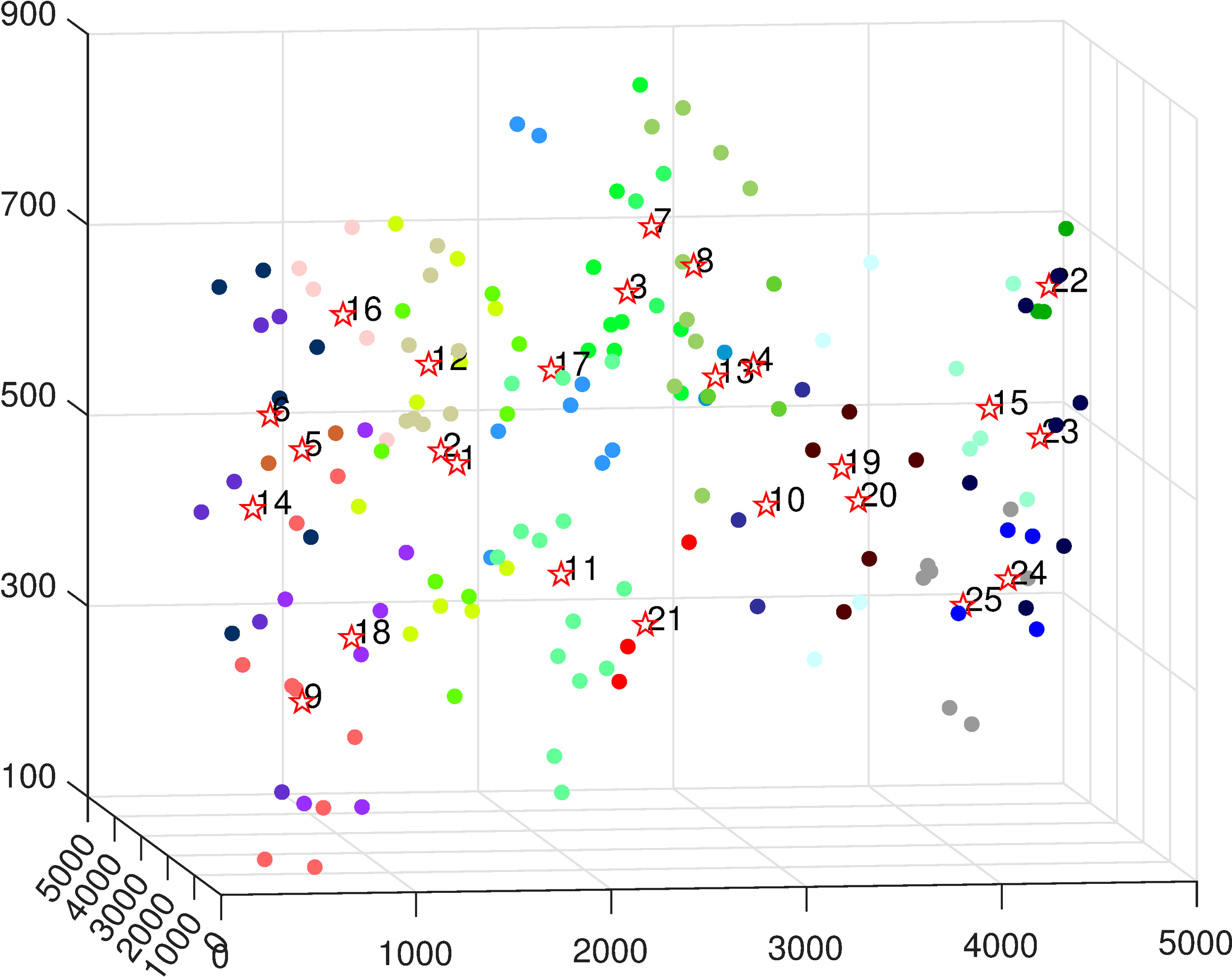
Figure 4. CK clustering result of 150 sensor nodes.

5.3 Performance comparison and analysis

To evaluate the performance of the proposed MADCS, we compare it with three benchmark algorithms, CKA-DPSO, LEACH-TSP, and DEKCS. CKA-DPSO is based on the cluster-based AUV scheduling data transmission protocol in Section 4.1, while applying DPSO algorithm to solve Problem P3 rather than the PGS algorithm. Given that LEACH (Heinzelman et al., 2002) is a data collection protocol without path planning, thus we add a path planning phase in LEACH. The path planning is formulated as a TSP problem that is solved by PGS. It is called LEACH-TSP. Moreover, the details of DEKCS are described in Omeke et al. (2021).

Obviously, the number of AUVs affects the average AoI. Since the CK algorithm divides the 150 sensor nodes into 25 clusters, we first study the trend of the average AoI with the number of AUVs varying from 1 to 25, as shown in Figure 5. In Figure 5A, it is difficult to distinguish the values of all average AoI under 1–25 AUVs in one graph because of the large span of average AoI values. For a clearer observation, we segregate Figure 5A into three figures, Figures 5B–D. They show the variation of average AoI at AUV numbers of 1–5, 6–15, and 16–25, respectively. As seen in Figure 5B, the average AoI decreases sharply when the number of AUVs increases from 1 to 2. It is because nearly half of the clusters are traversed by the other AUV, which means nearly half of the navigation time and uploading time is reduced, so that the average AoI curve is the steepest there. As the number of AUVs increases, the average AoI of four algorithms decreases. The explanation is that each AUV visits fewer HPs in its trajectory, so the packets wait for less time before arriving at the data center. Among the four data collection algorithms, the MADCS algorithm achieves the smallest average AoI under any number of AUVs, implying that the data are the freshest. In addition, we can find in Figure 5D that the average AoI is the same when 25 AUVs are dispatched to collaborate on data collection. Back to Figure 4, the sensors are grouped into 25 clusters, and each AUV visits one HP with a straight-line path when 25 AUVs are dispatched. Consequently, there is no difference between four algorithms in the case of 25 AUVs. Naturally, the average AoI is the same.

Figure 5

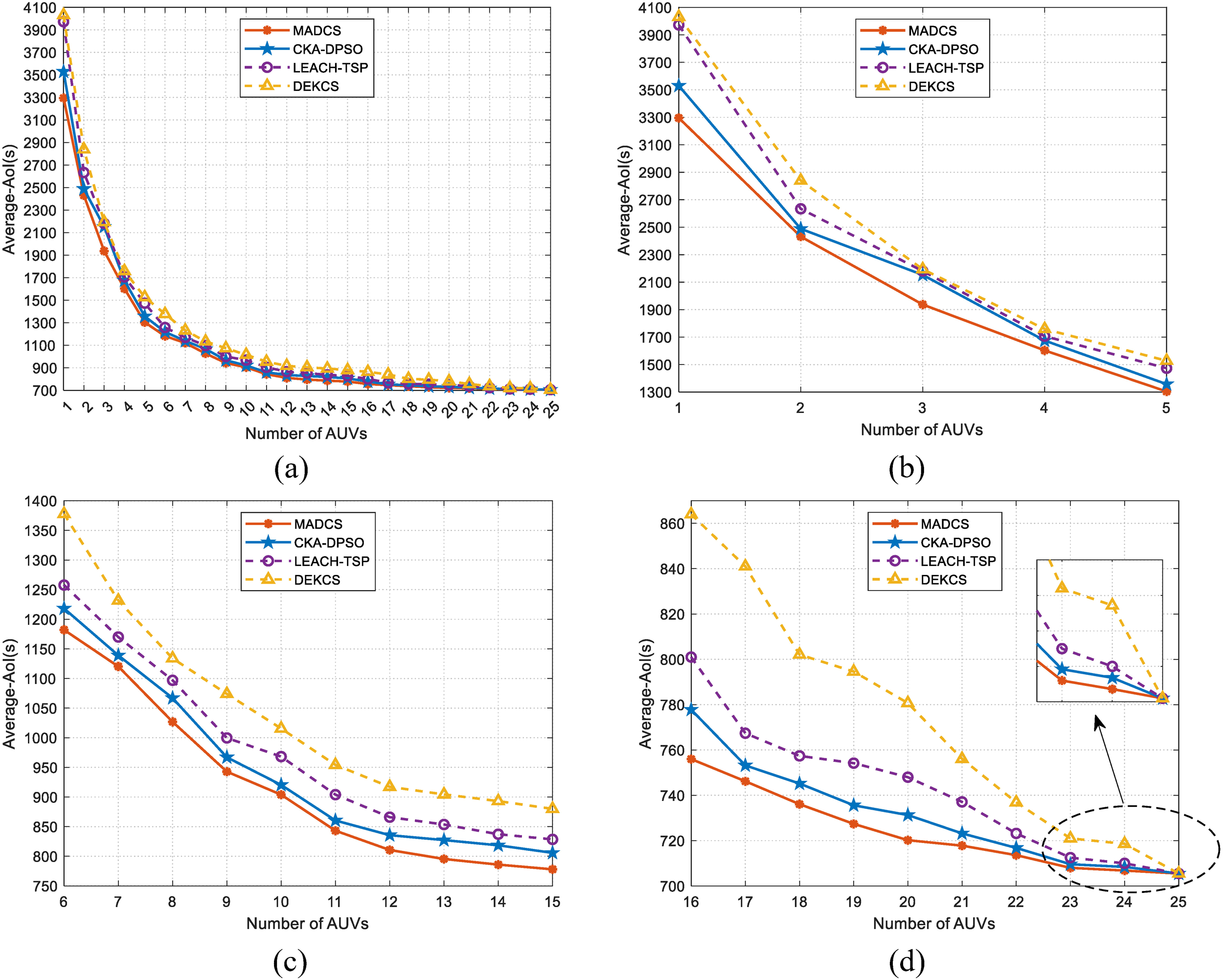
Figure 5. Average AoI with different number of AUVs, (a) 1-25, (b) 1-5, (c) 6-15, (d) 16-25.

Figure 6 shows how the AUVs’ total energy consumption is affected by the number of AUVs. We only chose several typical numbers to depict the tendency. It is seen that as the number of AUVs increases, the AUVs’ total energy consumption increases and tends to the same maximum value. Because more AUVs navigate greater distances, the total energy consumption increases. As the number of AUVs increases, the navigation energy consumption between HPs is constant, while each AUV consumes more energy to depart from and return to the data center. On the other hand, in the case of 25 AUVs, the energy consumption is the same among four algorithms, which has been analyzed before. Since the shortest path is considered in LEACH-TSP, it always consumes minimal energy, while MADCS comes in a close second. However, the proposed MADCS performs much better in average AoI than LEACH-TSP.

Figure 6

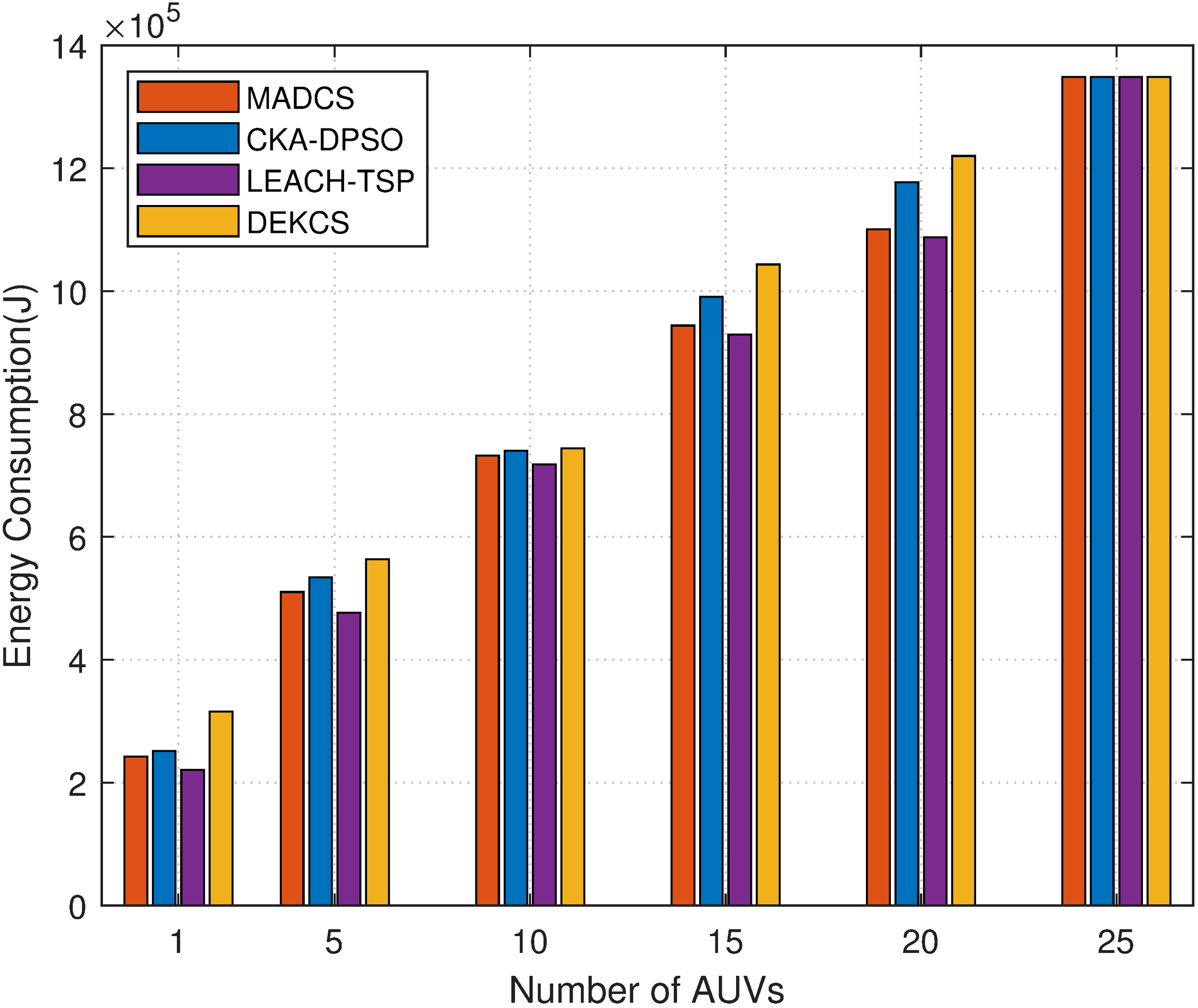
Figure 6. Energy consumption with different numbers of AUVs.

Next, we plot the relationship between the collection utility and the number of AUVs in Figure 7. We find that the proposed MADCS algorithm always holds a higher collection utility among four algorithms. This illustrates the effectiveness of the MADCS algorithm. Interestingly, the collection utility of different approaches increases with the rise of the number of AUVs and then decreases after reaching a peak value. The peak value is reached when the number of AUVs is 5. The justification behind this is that the collection delay decreases with the rise of AUVs’ number, leading to an improvement in the collection utility. However, more AUVs bring more energy consumption. Therefore, when continuing to increase the number of AUVs, the increase in energy consumption will outweigh the decrease in collection delay, which, in turn, degrades the collection utility.

Figure 7

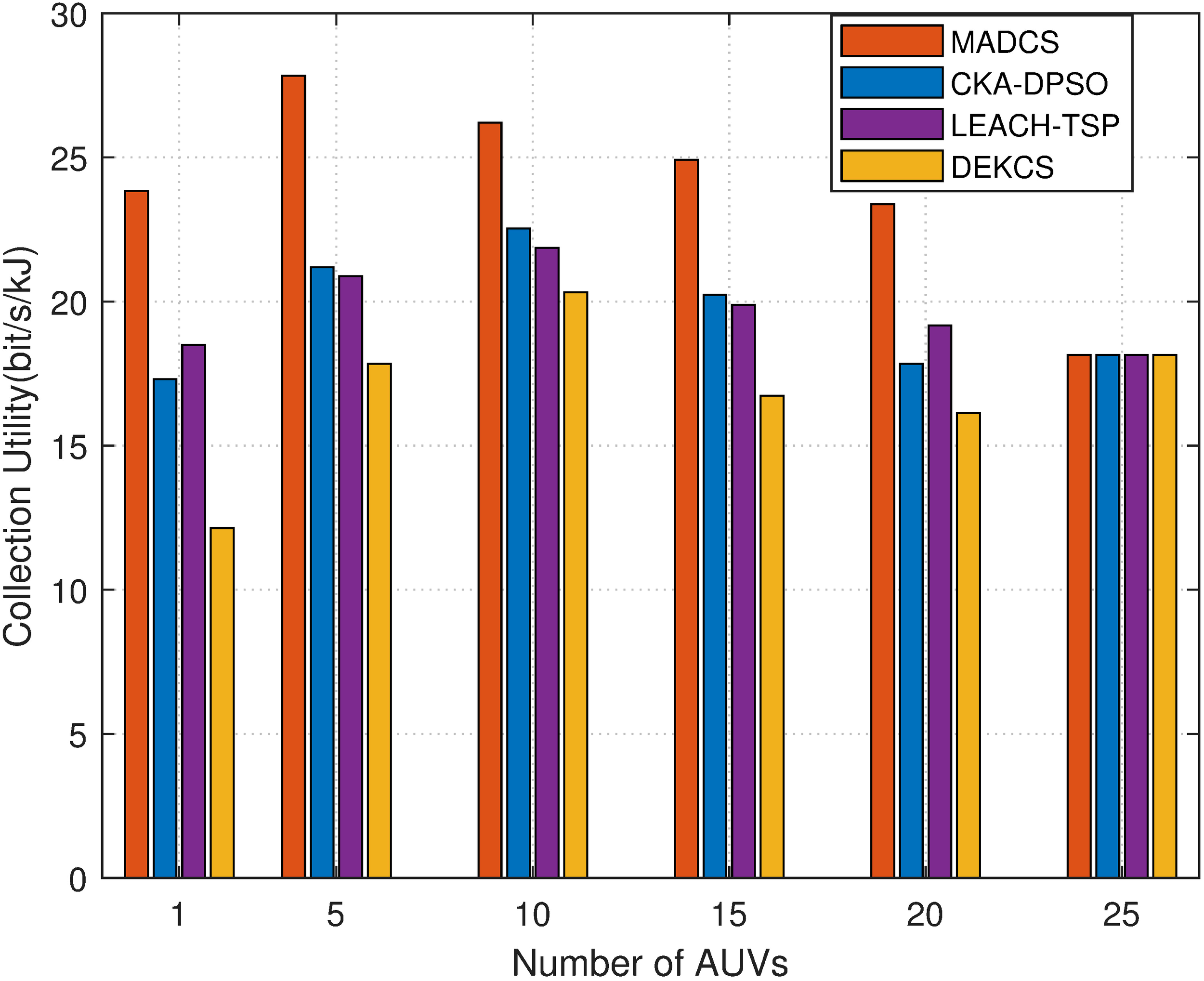
Figure 7. Collection utility with different numbers of AUVs.

We have investigated the performance of the four algorithms in terms of average AoI, energy consumption, and collection utility, and the proposed MADCS algorithm performs the best overall. In order to more intuitively demonstrate how the AUVs travel in the 3D scenario when the MADCS algorithm is applied, we show the trajectories of 1, 8, 16, and 25 AUVs under MADCS in Figures 8A, B, C, D, respectively. As shown in Figure 8, the number of HPs traversed by each AUV decreases with the AUVs increasing. Hence, the navigation time and hovering time of each AUV are reduced, which results in a smaller AoI. In the case of fewer than 25 AUVs, the trajectory of each AUV can be optimized, including the number of HPs visited by it and the traversal order. Yet, in the case of 25 AUVs, the trajectory of each AUV is fixed, i.e., every AUV visits only one HP, collecting data and then returning to the data center. It is the evidence why the above-mentioned indicators are the same in the case of 25 AUVs.

Figure 8

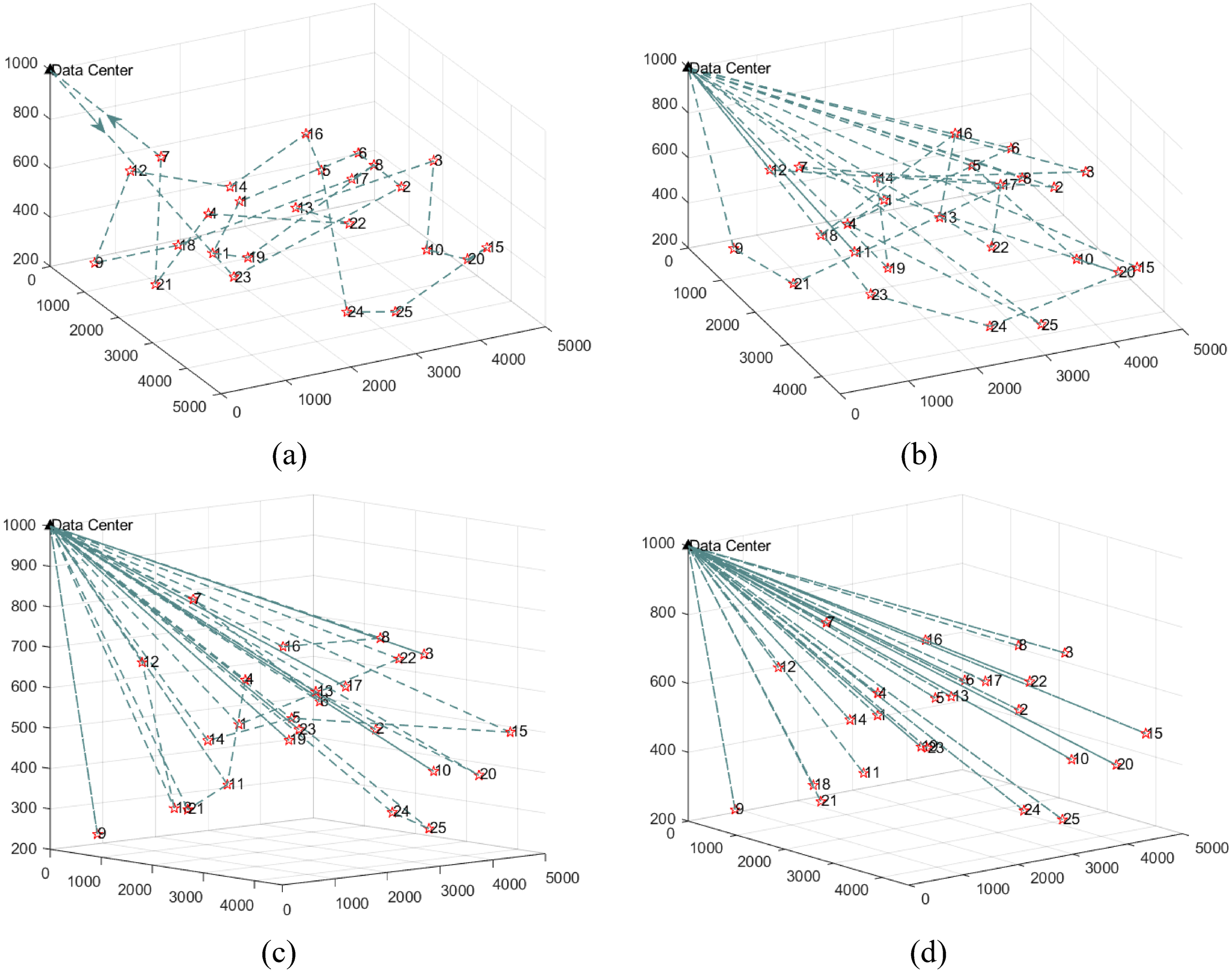
Figure 8. Trajectories of different number of AUVs under MADCS, (a) 1AUV, (b) 8AUVs, (c) 16AUVs, (d) 25AUVs.

In the previous analysis, we have mentioned that reducing energy consumption and average AoI simultaneously is difficult to do because they compete with each other. It is necessary to find the optimal trade-off between energy consumption and average AoI. Figure 9 depicts the Pareto frontiers for average AoI and energy consumption in MADCS. The results are consistent with the intuition that average AoI and energy consumption compete with each other. It is worth noticing that the Pareto points distribute sparsely and overlap, because both average AoI and energy consumption are functions of the AUVs’ trajectory, which is determined by discrete integer variables and thus cannot vary smoothly. Furthermore, generating an operating solution from the Pareto front is always meaningful in practice. As shown in Figure 9, the closest solution to the utopian point is dispatching five AUVs. Therefore, we choose five AUVs as the operating point and will analyze the impact of other factors on the performance of the MADCS algorithm in the case of five AUVs. The location and the performances of the operating point are marked with a black circle and rectangle, respectively, in Figure 9.

Figure 9

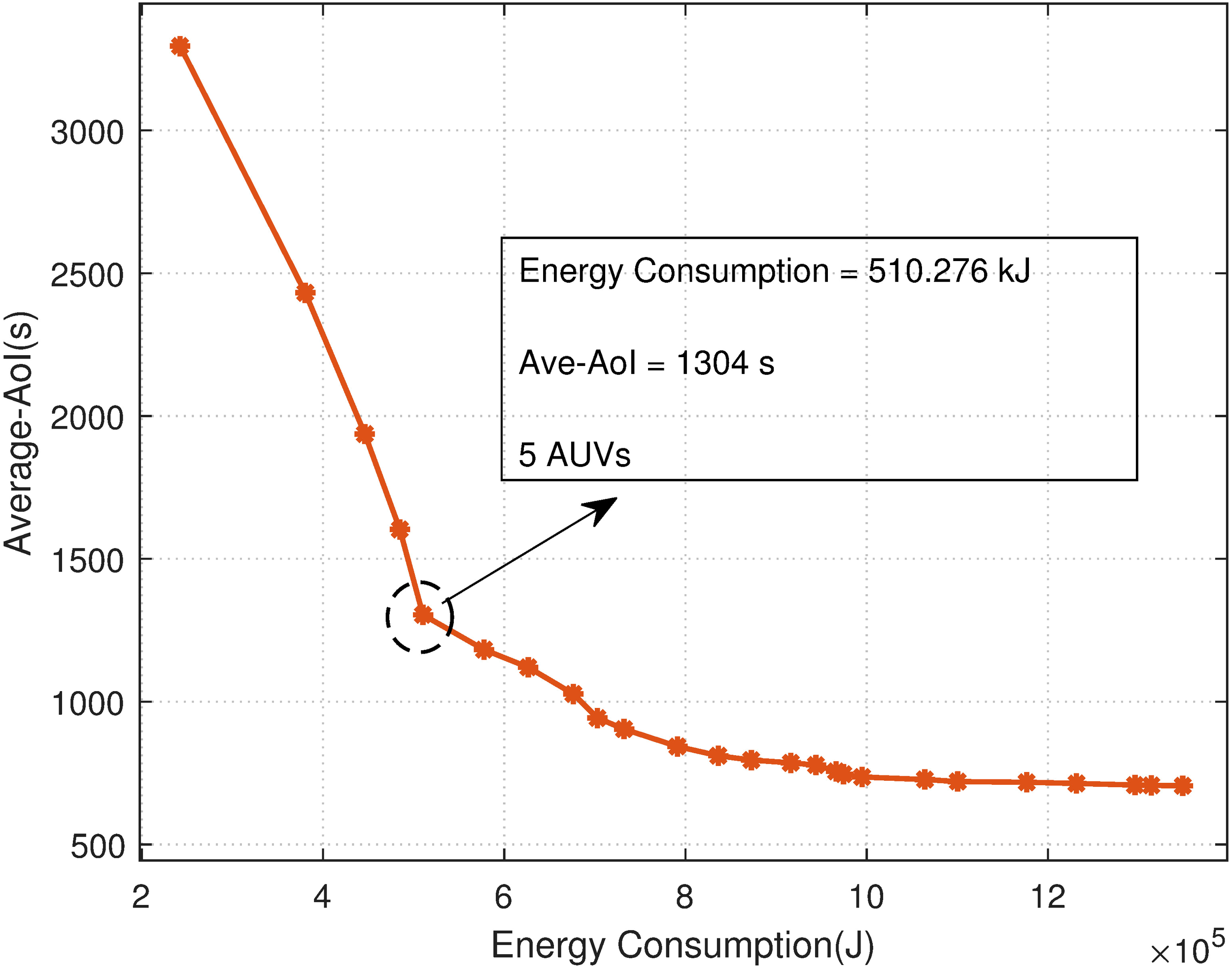
Figure 9. Pareto front for average AoI and energy consumption.

The velocity of AUVs affects their navigation time, which is correlated with AoI. Faster velocity requires higher propulsion power, leading to increased energy consumption. In the following experiment, we investigate the impact of AUV’s velocity on the performance of MADCS and the benchmark schemes. As shown in Figure 10, we compare the average AoI in different AUV velocities. Apparently, the average AoI of the four algorithms decreases as the velocity of AUVs increases. The greater the velocity of AUVs, the shorter the navigation time. Thus, the average AoI becomes smaller. In addition, the MADCS algorithm always holds the freshest average AoI under any velocity. It can be seen that the average AoI decreases sharper under small velocity than at large velocity. The reason is that the average AoI consists of navigation time and hovering time, while only the navigation time could be affected by the velocity of AUVs. When the velocity is small, the navigation time accounts for the majority of average AoI, whereas the collection time only accounts for a small portion. However, the situation reverses when in large velocity.

Figure 10

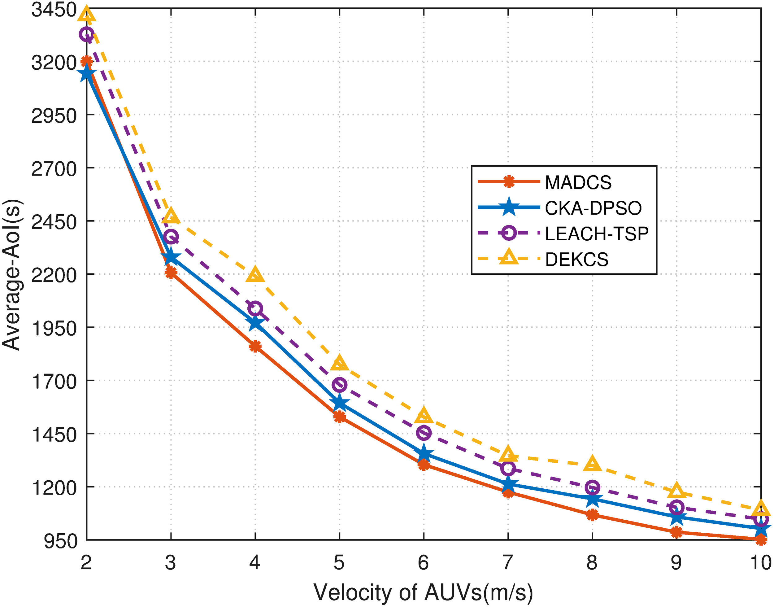
Figure 10. Average AoI with different velocities based on five AUVs.

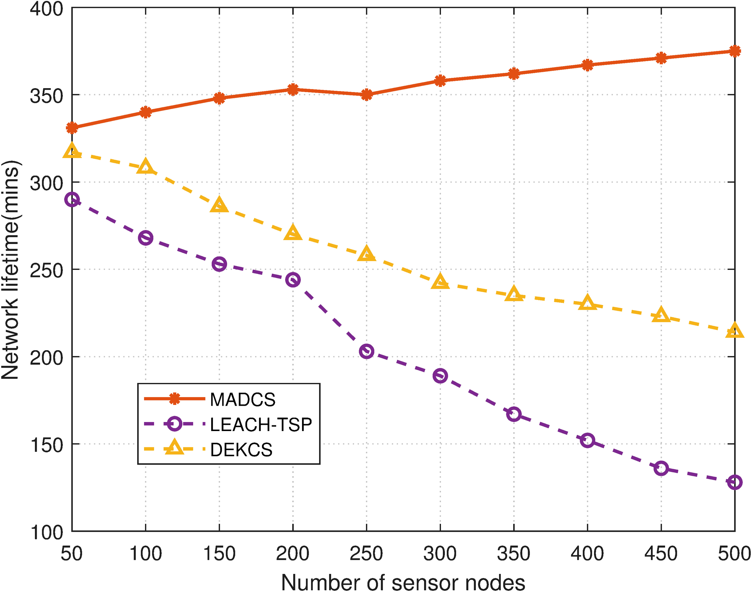
To demonstrate the effectiveness of the cluster-based AUV scheduling data transmission protocol, the performance of network lifetime and the residual energy standard deviation of sensors are explored. Network lifetime is defined as the duration until the first node runs out of its energy. CKA-DPSO differs from MADCS only in terms of path planning, so the performance of both metrics is the same. The network lifetime with different numbers of sensor nodes is shown in Figure 11, where MADCS, LEACH-TSP, and DEKCS are compared. From Figure 11, it can be seen that the network lifetime of MADCS increases with the number of sensor nodes, while the network lifetime of LEACH-TSP and DECKS decreases. The reason is as follows. In LEACH-TSP and DECKS, all the sensor nodes in the cluster transmit data to the cluster head, and then the cluster head transmits the data to the sink node and AUV, respectively. Sending the aggregated data of the whole cluster consumes a lot of energy of the cluster head. Moreover, when the network coverage area is fixed, the increase in the number of sensor nodes increases the node density. Then, the number of sensors in a cluster grows, which leads to the cluster heads spending more energy to collect and transmit data, thus reducing lifetime, whereas in MADCS, the AUV hovers at the cluster center position to act as a cluster head and the nodes within the cluster transmit data directly to the AUV. The energy consumption for secondary forwarding of data is saved. Therefore, the nodes consume less energy for data transmission than LEACH-TSP and DECKS and the network lifetime is extended. The distance between the nodes and AUVs is shortened as the number of nodes increases. Thus, the communication energy consumed by the nodes is reduced and the network lifetime is slightly increased.

Figure 11

Figure 11. Network lifetime for different numbers of nodes.

The residual energy standard deviation of sensors [i.e., σ_𝒮in Equation 12] is depicted in Figure 12. The performance of the proposed MADCS is relatively steady and also smaller than the other two algorithms. This is due to the fact that the nodes only transmit their data to AUVs directly, which not only saves but also balances the energy consumption of the sensor nodes. There are cluster heads in both LEACH-TSP and DECKS, which inevitably leads to uneven energy consumption.

Figure 12

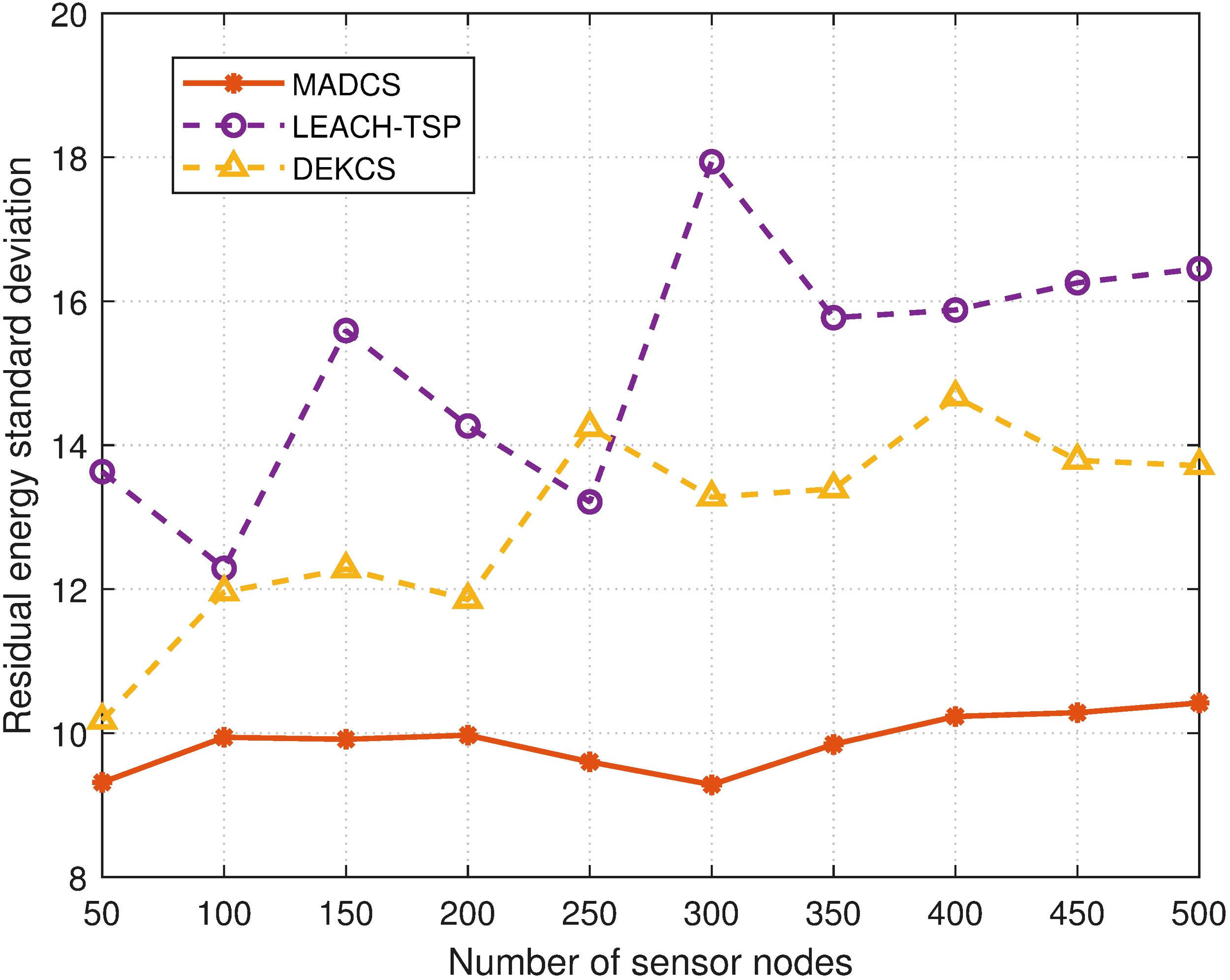
Figure 12. Residual energy standard deviation for different numbers of nodes.

6 Conclusion

In this paper, we investigate a multi-AUV-assisted underwater data collection framework for UASNs. In order to jointly optimize the AoI and energy consumption, we modeled it as a multi-objective MILP. A two-stage scheme MADCS, which consists of the cluster-based AUV scheduling data transmission protocol and the PGS-based trajectory planning algorithm, is proposed to solve the problem. Aiming at balancing and reducing the energy consumption of underwater sensors, the CK clustering algorithm is designed to make clustering more efficient and practical. The AUV scheduling-based transmission protocol is proposed to avoid packet collision and enhance channel utilization. According to the cluster-based network, trajectory for optimizing average AoI and energy consumption of AUV is planned through the proposed PGS algorithm. Simulation results validate that the proposed multi-AUV-assisted underwater data collection scheme outperforms three benchmark algorithms and achieves a proper trade-off between average AoI and energy consumption. We believe that the proposed multi-AUV-assisted underwater data collection scheme has potential application prospects in UASNs with demand for large-scale communication, large system capacity, long-term monitoring, and high data throughput. In future work, collaboration among multiple AUVs and trajectory optimization under real-time ocean currents will be considered.

Data availability statement

The original contributions presented in the study are included in the article/supplementary material. Further inquiries can be directed to the corresponding author.

Author contributions

WC: Conceptualization, Methodology, Writing – original draft, Writing – review & editing, Validation, Visualization. KC: Writing – review & editing, Methodology, Funding acquisition. EC: Funding acquisition, Supervision, Writing – review & editing.

Funding

The author(s) declare that financial support was received for the research and/or publication of this article. This work was supported in part by the National Natural Science Foundation of China (NSFC) under Grant Nos. 62271425, U24A20215, and 62071402.

Conflict of interest

The authors declare that the research was conducted in the absence of any commercial or financial relationships that could be construed as a potential conflict of interest.

Generative AI statement

The author(s) declare that no Generative AI was used in the creation of this manuscript.

Publisher’s note

All claims expressed in this article are solely those of the authors and do not necessarily represent those of their affiliated organizations, or those of the publisher, the editors and the reviewers. Any product that may be evaluated in this article, or claim that may be made by its manufacturer, is not guaranteed or endorsed by the publisher.

References

Abd-Elmagid M. A. and Dhillon H. S. (2018). Average peak age-of-information minimization in uav-assisted iot networks. IEEE Trans. Vehicular Technol. 68, 2003–2008. doi: 10.1109/TVT.25

Crossref Full Text | Google Scholar

Abhishek B., Ranjit S., Shankar T., Eappen G., Sivasankar P., and Rajesh A. (2020). Hybrid pso-hsa and pso-ga algorithm for 3d path planning in autonomous uavs. SN Appl. Sci. 2, 1–16. doi: 10.1007/s42452-020-03498-0

Crossref Full Text | Google Scholar

Al-Habob A. A., Dobre O. A., and Poor H. V. (2021). Age-optimal information gathering in linear underwater networks: A deep reinforcement learning approach. IEEE Trans. Vehicular Technol. 70, 13129–13138. doi: 10.1109/TVT.2021.3117536

Crossref Full Text | Google Scholar

Anuradha D., Subramani N., Khalaf O. I., Alotaibi Y., Alghamdi S., and Rajagopal M. (20222867). Chaotic search-and-rescue-optimization-based multi-hop data transmission protocol for underwater wireless sensor networks. Sensors 22. doi: 10.3390/s22082867

PubMed Abstract | Crossref Full Text | Google Scholar

Brekhovskikh L. M., Lysanov Y. P., and Lysanov J. P. (2003). Fundamentals of ocean acoustics (New York, NY, USA: Springer Science & Business Media).

Google Scholar

Chaitanya D. E., Sridevi C. V., and Rao G. S. B. (2011). “Path loss analysis of underwater communication systems,” in IEEE technology students’ Symposium (Kharagpur, India: IEEE), 65–70.

Google Scholar

Cruz N. A. (2019). “Optimizing the power budget of hovering auvs,” in 2019 IEEE underwater technology (UT) (Kaohsiung, Taiwan: IEEE), 1–6.

Google Scholar

de Souza F. A., Chang B. S., Brante G., Souza R. D., Pellenz M. E., and Rosas F. (2016). Optimizing the number of hops and retransmissions for energy efficient multi-hop underwater acoustic communications. IEEE Sensors J. 16, 3927–3938. doi: 10.1109/JSEN.2016.2532384

Crossref Full Text | Google Scholar

EvoLogics (2023). Evologics acoustic modems technical specifications. Available online at: https://www.evologics.com/product/s2c-r-18-34-1.

Google Scholar

Fang Z., Wang J., Jiang C., Zhang Q., and Ren Y. (2021). Aoi-inspired collaborative information collection for auv-assisted internet of underwater things. IEEE Internet Things J. 814571. doi: 10.1109/JIOT.2021.3049239

Crossref Full Text | Google Scholar

Favaro F., Brolo L., Toso G., Casari P., and Zorzi M. (2013). “A study on remote data retrieval strategies in underwater acoustic networks,” in 2013 OCEANS-san diego (San Diego, CA, USA: IEEE), 1–8.

Google Scholar

Gjanci P., Petrioli C., Basagni S., Phillips C. A., Bölöni L., and Turgut D. (2017). Path finding for maximum value of information in multi-modal underwater wireless sensor networks. IEEE Trans. Mobile Computing 17, 404–418. doi: 10.1109/TMC.2017.2706689

Crossref Full Text | Google Scholar

Guan Q., Ji F., Liu Y., Yu H., and Chen W. (2019). Distance-vector-based opportunistic routing for underwater acoustic sensor networks. IEEE Internet Things J. 6, 3831–3839. doi: 10.1109/JIoT.6488907

Crossref Full Text | Google Scholar

Han G., Gong A., Wang H., Martínez-García M., and Peng Y. (2021). Multi-auv collaborative data collection algorithm based on q-learning in underwater acoustic sensor networks. IEEE Trans. Vehicular Technol. 70, 9294–9305. doi: 10.1109/TVT.2021.3097084

Crossref Full Text | Google Scholar

Han G., Long X., Zhu C., Guizani M., Bi Y., and Zhang W. (2019). An auv location prediction-based data collection scheme for underwater wireless sensor networks. IEEE Trans. Vehicular Technol. 68, 6037–6049. doi: 10.1109/TVT.25

Crossref Full Text | Google Scholar

Han G., Shen S., Song H., Yang T., and Zhang W. (2018). A stratification-based data collection scheme in underwater acoustic sensor networks. IEEE Trans. Vehicular Technol. 67, 10671–10682. doi: 10.1109/TVT.2018.2867021

Crossref Full Text | Google Scholar

Hao Z., Li W., and Zhang Q. (2023). “Efficient clustering data collection in auv-aided underwater sensor network,” in OCEANS 2023-MTS/IEEE US gulf coast (Biloxi, MS, USA: IEEE), 1–6.

Google Scholar

Heinzelman W. B., Chandrakasan A. P., and Balakrishnan H. (2002). An application-specific protocol architecture for wireless microsensor networks. IEEE Trans. wireless Commun. 1, 660–670. doi: 10.1109/TWC.2002.804190

Crossref Full Text | Google Scholar

Hollinger G. A., Yerramalli S., Singh S., Mitra U., and Sukhatme G. S. (2011). “Distributed coordination and data fusion for underwater search,” in 2011 IEEE international conference on robotics and automation (Shanghai, China: IEEE), 349–355.

Google Scholar

Hou X., Wang J., Bai T., Deng Y., Ren Y., and Hanzo L. (2022). Environment-aware auv trajectory design and resource management for multi-tier underwater computing. IEEE J. Selected Areas Commun. 41, 474–490. doi: 10.1109/JSAC.2022.3227103

Crossref Full Text | Google Scholar

Hwang D. and Kim D. (2008). “Dfr: Directional flooding-based routing protocol for underwater sensor networks,” in OCEANS, vol. 2008. (Quebec City, QC, Canada: IEEE), 1–7.

Google Scholar

Jiang B., Du J., Jiang C., Han Z., and Debbah M. (2024). Underwater searching and multiround data collection via auv swarms: An energy-efficient aoi-aware mappo approach. IEEE Internet Things J. 11, 12768–12782. doi: 10.1109/JIOT.2023.3336055

Crossref Full Text | Google Scholar

Kaul S., Yates R., and Gruteser M. (2012). “Real-time status: How often should one update?,” in In 2012 proceedings IEEE INFOCOM (Orlando, FL, USA: IEEE), 2731–2735.

Google Scholar

Khan Z. U., Aman M., Rahman W. U., Khan F., Jamil T., and Hashim R. (2023). “Machine learningbased multi-path reliable and energy-efficient routing protocol for underwater wireless sensor networks,” in 2023 international conference on frontiers of information technology (FIT) (Islamabad, Pakistan: IEEE), 316–321.

Google Scholar

Khan M. T. R., Jembre Y. Z., Ahmed S. H., Seo J., and Kim D. (2019). “Data freshness based auv path planning for uwsn in the internet of underwater things,” in 2019 IEEE global communications conference (GLOBECOM) (Waikoloa, HI, USA: IEEE), 1–6.

Google Scholar

Khan S. U., Khan Z. U., Alkhowaiter M., Khan J., and Ullah S. (2024). Energy-efficient routing protocols for uwsns: A comprehensive review of taxonomy, challenges, opportunities, future research directions, and machine learning perspectives. J. King Saud University-Computer Inf. Sci. 102128. doi: 10.1016/j.jksuci.2024.102128

Crossref Full Text | Google Scholar

Li Y., Huang H., Zhuang Y., Zhong Z., Wang C.-X., and Wang X. (2023). An auv-assisted data collection scheme for uwsns based on reinforcement learning under the influence of ocean current. IEEE Sensors J. 24, 3960–3972. doi: 10.1109/JSEN.2023.3339155

Crossref Full Text | Google Scholar

Li N., Martínez J.-F., Meneses Chaus J. M., and Eckert M. (2016). A survey on underwater acoustic sensor network routing protocols. Sensors 16, 414. doi: 10.3390/s16030414

PubMed Abstract | Crossref Full Text | Google Scholar

Lin S., Liu A., Wang J., and Kong X. (2023). An intelligence-based hybrid pso-sa for mobile robot path planning in warehouse. J. Comput. Sci. 67, 101938. doi: 10.1016/j.jocs.2022.101938

Crossref Full Text | Google Scholar

Liu J., Tong P., Wang X., Bai B., and Dai H. (2020a). Uav-aided data collection for information freshness in wireless sensor networks. IEEE Trans. Wireless Commun. 20, 2368–2382. doi: 10.1109/TWC.2020.3041750

Crossref Full Text | Google Scholar

Liu J., Tong P., Wang X., Bai B., and Dai H. (2020b). Uav-aided data collection for information freshness in wireless sensor networks. IEEE Trans. Wireless Commun. 20, 2368–2382. doi: 10.1109/TWC.2020.3041750

Crossref Full Text | Google Scholar

Luo H., Xu Z., Wang J., Yang Y., Ruby R., and Wu K. (2022). Reinforcement learning-based adaptive switching scheme for hybrid optical-acoustic auv mobile network. Wireless Commun. Mobile Computing 2022. doi: 10.1155/2022/9471698

Crossref Full Text | Google Scholar

National Research Council, Division on Earth, Life Studies, Ocean Studies Board, and Committee on Exploration of the Seas. (2003). Exploration of the seas: voyage into the unknown (Washington, DC, USA: National Academies Press).

Google Scholar

Omeke K. G., Mollel M. S., Ozturk M., Ansari S., Zhang L., Abbasi Q. H., et al. (2021). Dekcs: A dynamic clustering protocol to prolong underwater sensor networks. IEEE Sensors J. 21, 9457–9464. doi: 10.1109/JSEN.7361

Crossref Full Text | Google Scholar

Qiu T., Zhao Z., Zhang T., Chen C., and Chen C. P. (2019). Underwater internet of things in smart ocean: System architecture and open issues. IEEE Trans. Ind. Inf. 16, 4297–4307. doi: 10.1109/TII.2019.2946618

Crossref Full Text | Google Scholar

Rahman W. U., Gang Q., Feng Z., Khan Z. U., Aman M., and Ullah I. (2023). “A q-learning-based multihop energy-efficient and low collision mac protocol for underwater acoustic wireless sensor networks,” in In 2023 20th International Bhurban Conference on Applied Sciences and Technology (IBCAST), Bhurban, Murree, Pakistan, pp. 872–877. doi: 10.1109/IBCAST59916.2023.10712998

Crossref Full Text | Google Scholar

Roberge V., Tarbouchi M., and Labonté G. (2012). Comparison of parallel genetic algorithm and particle swarm optimization for real-time uav path planning. IEEE Trans. Ind. Inf. 9, 132–141. doi: 10.1109/TII.2012.2198665

Crossref Full Text | Google Scholar

Stojanovic M. (2007). On the relationship between capacity and distance in an underwater acoustic communication channel. ACM SIGMOBILE Mobile Computing Commun. Rev. 11, 34–43. doi: 10.1145/1347364.1347373

Crossref Full Text | Google Scholar

Su R., Zhang D., Li C., Gong Z., Venkatesan R., and Jiang F. (2019). Localization and data collection in auv-aided underwater sensor networks: Challenges and opportunities. IEEE Network 33, 86–93. doi: 10.1109/MNET.2019.1800425

Crossref Full Text | Google Scholar

Talak R., Karaman S., and Modiano E. (2018). Optimizing information freshness in wireless networks under general interference constraints. In. Proc. Eighteenth ACM Int. Symposium Mobile Ad Hoc Networking Computing., 61–70. doi: 10.1145/3209582

Crossref Full Text | Google Scholar

ur Rahman W., Gang Q., Feng Z., Khan Z. U., Aman M., and Bilal M. (2023). “A maca-based energy-efficient mac protocol using q-learning technique for underwater acoustic sensor network,” in 2023 IEEE 11th international conference on computer science and network technology (ICCSNT) (Dalian, China: IEEE), 352–355.

Google Scholar

Wang Y., Tian Z., Sun Y., Du X., and Guizani N. (2020). Preserving location privacy in uasn through collaboration and semantic encapsulation. IEEE Network 34, 284–290. doi: 10.1109/MNET.65

Crossref Full Text | Google Scholar

Wang T., Zhao D., Cai S., Jia W., and Liu A. (2019). Bidirectional prediction-based underwater data collection protocol for end-edge-cloud orchestrated system. IEEE Trans. Ind. Inf. 16, 4791–4799. doi: 10.1109/TII.9424

Crossref Full Text | Google Scholar

Xu J., Zhang Z., Wang Z., Wang J., and Rent Y. (2024). “Vol and energy-aware auv-assisted data collection for internet of underwater things,” in 2024 IEEE wireless communications and networking conference (WCNC) (Dubai, United Arab Emirates: IEEE), 1–6.

Google Scholar

Yang Y., Xiao Y., and Li T. (2021). A survey of autonomous underwater vehicle formation: Performance, formation control, and communication capability. IEEE Commun. Surveys Tutorials 23, 815–841. doi: 10.1109/COMST.2021.3059998

Crossref Full Text | Google Scholar

Yu W., Chen Y., Wan L., Zhang X., Zhu P., and Xu X. (2020). An energy optimization clustering scheme for multi-hop underwater acoustic cooperative sensor networks. IEEE Access 8, 89171–89184. doi: 10.1109/Access.6287639

Crossref Full Text | Google Scholar

Zhang S., Zhang H., Han Z., Poor H. V., and Song L. (2020). Age of information in a cellular internet of uavs: Sensing and communication trade-off design. IEEE Trans. Wireless Commun. 19, 6578–6592. doi: 10.1109/TWC.7693

Crossref Full Text | Google Scholar

Zhao C., Feng B., and Zhang Q. (2021). “Mobile sink leach protocol for underwater acoustic sensor networks,” in 2021 13th international conference on wireless communications and signal processing (WCSP) (Changsha, China: IEEE), 1–6.

Google Scholar

Zhuo X., Liu M., Wei Y., Yu G., Qu F., and Sun R. (2020). Auv-aided energy-efficient data collection in underwater acoustic sensor networks. IEEE Internet Things J. 7, 10010–10022. doi: 10.1109/JIoT.6488907

Crossref Full Text | Google Scholar

Appendix 1. Proof of proposition 1

According to Equation 17, the AoI of the jth sensor node in the last cluster of the AUV v_k’s trajectory is:

$$A_{(M^k),(j)}^{(k)}=\sum _{i=j}^{\left|{\mathcal{J}}_{(M^k)}\right|}{\theta }_{(M^k),(i)}+{\lambda }_{(M^k),(M^k+1)}$$

Thus, the overall AoI of sensors in the last cluster of the AUV v_k’s trajectory is:

$$\begin{array}{ll}{A}_{(M^k)}^k\hfill & =\sum _{j=1}^{\left|{\mathcal{J}}_{(M^k)}\right|}\left(\sum _{i=j}^{\left|{\mathcal{J}}_{(M^k)}\right|}{\theta }_{(M^k),(i)}+{\lambda }_{(M^k),(M^k+1)}\right)=\sum _{j=1}^{\left|{\mathcal{J}}_{(M^k)}\right|}j{\theta }_{(M^k),(j)}+\left|{\mathcal{J}}_{(M^k)}\right|{\lambda }_{(M^k),(M^k+1)}\hfill \end{array}$$

Likewise, the overall AoI of sensors in the mth cluster of the AUV v_k’s trajectory is:

$$\begin{array}{l}{A}_{(m)}^k=\sum _{j=1}^{\left|{\mathcal{J}}_{(m)}\right|}\left(\sum _{i=j}^{\left|{\mathcal{J}}_{(m)}\right|}{\theta }_{(m),(i)}+\sum _{i=m}^{M^k}{\lambda }_{(i),(i+1)}+\sum _{l=m+1}^{M^k}\sum _{i=1}^{\left|{\mathcal{J}}_{(l)}\right|}{\theta }_{(l),(i)}\right)\\ =\left|{\mathcal{J}}_{(m)}\right|\left(\sum _{l=m+1}^{M^k}{\psi }^{(l)}+\sum _{i=m}^{M^k}{\lambda }_{(i),(i+1)}\right)+\sum _{j=1}^{\left|{\mathcal{J}}_{(m)}\right|}j{\theta }_{(m),(j)}\end{array}$$

where ${\psi }^{(l)}={\sum }_{i=1}^{\left|{\mathcal{J}}_{(l)}\right|}{\theta }_{(l),(i)}$ denotes the total amount of uploading time of the sensors in the lth cluster visited by v_k. Then, the above equation can be used to derive the sum AoI of all sensors collected by AUV v_k:

$$\begin{array}{l}{A}^k=\sum _{m=1}^{M^k}{A}_{(m)}^k\\ =\sum _{m=1}^{M^k}\sum _{j=1}^{\left|{\mathcal{J}}_{(m)}\right|}j{\theta }_{(m),(j)}+\sum _{m=1}^{M^k}\left|{\mathcal{J}}_{(m)}\right|\sum _{l=m+1}^{M^k}{\psi }^{(l)}+\sum _{i=1}^{M^k}\left(\sum _{m=1}^i\left|{\mathcal{J}}_{(m)}\right|\right){\lambda }_{(i),(i+1)}\\ =\sum _{m=1}^{M^k}\sum _{j=1}^{\left|{\mathcal{J}}_{(m)}\right|}j{\theta }_{(m),(j)}+\sum _{m=2}^{M^k}\left(\sum _{l=1}^{m-1}\left|{\mathcal{J}}_{(l)}\right|\right){\psi }^{(m)}+\sum _{i=1}^{M^k}\left(\sum _{m=1}^i\left|{\mathcal{J}}_{(m)}\right|\right){\lambda }_{(i),(i+1)}\end{array}$$

We further define ${\xi }^{(l)}={\sum }_{i=1}^l\left|{\mathcal{J}}_{(i)}\right|$ as the number of sensors visited from the first cluster to the lth cluster in the trajectory of v_k. Thus, we can get:

$$\begin{array}{ll}{A}^k\hfill & =\sum _{m=2}^{M^k}{\xi }^{m-1}{\psi }^{(m)}+\sum _{i=1}^{M^k}{\xi }^i{\lambda }_{(i),(i+1)}+\sum _{m=1}^{M^k}\sum _{j=1}^{\left|{\mathcal{J}}_{(m)}\right|}j{\theta }_{(m),(j)}\hfill \end{array}$$

As a result, the proof of Proposition 1 is completed.

Appendix 2. Cluster validity indices

Let $X=\left\{x_1,x_2,\cdots ,x_n\right\}$ be the dataset containing n sensor nodes in a 3D space, and $x_i\in R^3$. $Z_1,Z_2,\cdots ,Z_c$ are c disjoint subsets of X, i.e., clusters. $n_1,n_2,\cdots ,n_c$ are the number of sensor nodes that belong to the corresponding cluster, thus ${\displaystyle {\sum }_{i=1}^c{n}_i=n.o_1,o_2,\cdots ,o_c}$ denote the centroid of Z_i and O is the global centroid. d(i,j) is defined as the Euclidean distance between node i and j.

1. The silhouette coefficient can be expressed as:

$$SI=\frac{1}{N}\sum _{k=1}^N\frac{b(x_i)-a(x_i)}{\text{max} \{a(x_i),b(x_i)\}}$$

where $a(x_i)$ represents the cohesiveness of the sensor nodes and denotes the average distance among x_i and other sensor nodes in the same cluster. b(x_i) represents the average distance from sensor node x_i to all sensor nodes in another most adjacent cluster:

$$a(x_i)=\frac{1}{n_k-1}\sum _{x_i,x_j\in Z_k,i\ne j}d(x_i,x_j)$$

$$b(x_i)=\underset{Z_k\ne Z_l}{\min }\frac{1}{\left|n_l\right|}\sum _{x_i\in Z_k,x_j\in Z_l}d(x_i,x_j)$$

Observing from the formula, we get that SI ∈ [−1,1] and the index closer to 1 refers to a better partition.

2. The Calinski–Harabasz index can be expressed as:

$$\text{CHI}=\frac{n-c}{c-1}·\frac{{\sum }_{j=1}^c{n}_{j}d{(o_j,O)}^2}{{\sum }_{j=1}^c{\sum }_{i=1}^{n_j}d{(x_i,o_j)}^2}$$

where the numerator represents the separation among clusters and the denominator represents the compactness of a cluster. Thus, the larger index refers to a better partition.

3. The Davies–Bouldin index can be expressed as:

$$DBI=\frac{1}{c}\sum _{k,l=1}^c\underset{k\ne l}{\text{max }}{R}_{kl}$$

where R_kl represents the similarity among clusters, which is $R_{kl}=\frac{D_k+D_l}{d(O_k,O_l)}.D_k$ is the diameter of a cluster, the expression is:

$$D_k=\frac{1}{n_k}\sum _{i=1}^{n_k}d(x_i,o_k)$$

The value range of DBI is [0,+∞] and the index closer to 0 refers to a better partition.