Biophysical model of eelgrass and water quality in Coos Bay, OR shows greater mitigation potential for ocean acidification than hypoxia

Seagrass beds provide important ecosystem services and are valued, in part, for their potential to mediate stressors such as ocean acidification and hypoxia (OAH) for sensitive species. However, the susceptibility of seagrasses to anthropogenic impacts and recent declines motivate the need to better understand the drivers of seagrass and the water quality consequences that occur with variation in seagrass abundance. To meet this need, we leveraged existing monitoring data (water quality and seagrass), hydrodynamic circulation model, and biogeochemical model framework with seagrass submodel, to produce a biophysical model of Coos Bay estuary, Oregon, U.S. The model includes biogeochemical processes involving water quality, plankton, seagrass, and sediment-water interactions. Ecosystem models like this are useful for evaluating complex estuarine systems because they allow us to extend our understanding of system dynamics beyond existing observations and perform experiments to identify the processes driving observed patterns. We used the biophysical model of Coos Bay to evaluate the dynamics of water quality and native eelgrass (Zostera marina) under three eelgrass abundance scenarios (zero eelgrass, current extent, and maximum observed extent) to elucidate the relationship between eelgrass and OAH. Including eelgrass in the Coos Bay model produced results that more closely resembled water quality observations - dissolved oxygen (DO) and pH were more dynamic in simulations with eelgrass, often having both higher highs and lower lows. While there were some areas of the estuary where DO improved with the addition of eelgrass to the model there was overall a small net increase in harmful DO conditions (based on a salmon physiological threshold). In contrast, ocean acidification conditions, pH and calcium carbonate saturation state for aragonite (Ω), were improved (based on oyster requirements) with the addition of eelgrass - although the magnitude of improvement differed seasonally and spatially. Our new model represents a useful tool - one which accounts for and controls the relevant physical and biogeochemical processes - to evaluate conditions that confer resilience or enhance vulnerability to OAH in an important Pacific Northwest coastal estuary and results can inform the OAH-related dynamics occurring in other eastern boundary current estuaries.

1 Introduction

Estuarine ecosystems provide important services to coastal communities (Barbier et al., 2011). Despite their value, critical estuarine habitats, including seagrass beds, are being degraded by anthropogenic impacts such as land-based nutrients and pollutants, invasive species, climate change, and overharvesting (Kennish, 2021). Seagrasses are one of the most valuable ecosystems in terms of the services provided (Costanza et al., 1997) and they contribute to the functioning of estuaries as habitat, by altering sediment dynamics, and through their tight link with water quality. For instance, these primary producers both influence, and are influenced by, water column nutrients (Valiela, 1995; Lincoln et al., 2021), carbon (Koch et al., 2013), sediment (Walter et al., 2020), and dissolved oxygen (DO) (Long et al., 2020). Because of their influence on carbon and DO, seagrass conservation and restoration are proposed mitigation strategies for ocean acidification and hypoxia (referred to together as OAH), which are threats characterized by water that is acidified (CO₂-rich, low pH) and low DO, respectively (Feely et al., 2016). These often co-occurring phenomena are increasing in frequency and severity (Grantham et al., 2004). However, researchers and managers are still trying to understand the scales at which OAH mitigation by seagrass can be realized, how mitigation varies with abundance, and where mitigation might be most impactful.

Ocean acidification and hypoxia negatively impact many marine and estuarine organisms, with cascading effects on broader ecological interactions (e.g., Bednaršek et al., 2020; Klinger et al., 2017; Sampaio et al., 2021). Generally, estuaries are more susceptible to OAH compared to the open ocean (Waldbusser and Salisbury, 2014) because the natural buffering capacity of ocean waters is reduced due to dilution with low-alkalinity freshwater, eutrophication, and high metabolic rates (Pacella et al., 2018, 2024). U.S. Pacific Northwest (PNW) estuaries are disproportionately vulnerable because ocean upwelling naturally brings CO₂-rich, low pH, and low DO water to the coastal zone (Gruber et al., 2012) and close ocean-estuary coupling readily moves the acidified and low DO water into estuaries (Brown and Ozretich, 2009). There are consequences of OAH for ecologically and economically important PNW fisheries, especially shellfish, and other estuarine ecosystem services (Barton et al., 2012; Marshall et al., 2018).

Seagrasses are proposed to mitigate OAH during photosynthesis via the uptake of inorganic carbon and release of DO leading to increased pH and DO, decreased partial pressure of carbon dioxide (pCO₂), and improved carbonate mineral saturation state in the surrounding waters (Hendriks et al., 2014). This results in diel cycles in DO, pH, and pCO₂ that are coincident with the daily cycle of photosynthesis and respiration (Magel et al., 2023). Seagrasses are thought to have large mitigation potential, in part because of their high productivity (Duarte and Cebrian, 1996), and a growing number of studies have found that estuarine seagrasses, including native PNW eelgrass Zostera marina, have local effects on carbonate chemistry and DO (Pacella et al., 2018; Ricart et al., 2021; Magel et al., 2023). However, the magnitude and direction of the effect of seagrass on pH and DO are still debated (Koweek et al., 2018; Van Dam et al., 2021a). Concurrently, seagrass declines are accelerating worldwide, with thermal stress, eutrophication, disturbance, and disease often cited as causes (Waycott et al., 2009; Unsworth and Cullen-Unsworth, 2014). Recently in the PNW, declining eelgrass abundance in a protected region of Coos Bay, Oregon has highlighted the need to understand the consequences of eelgrass variability for estuarine water quality, including OAH mitigation (Magel et al., 2023). Partial to complete loss of eelgrass, depending on the location within the estuary, began in 2015 and was primarily associated with increased temperatures from a marine heatwave and reduced light availability from increased watershed disturbance may have also contributed (Magel et al., 2023; Marin Jarrin et al., 2022).

Various methods have been used to measure OAH mitigation by seagrasses, including mesocosm studies (Bergstrom et al., 2019; Liu et al., 2020), comparisons inside versus outside of seagrass beds (Hendriks et al., 2014; Ricart et al., 2021), and interannual variability in seagrass abundance (Magel et al., 2023). Modeling studies have also explored seagrass mitigation of OAH using a simple box model (Koweek et al., 2018), deterministic model (Pacella et al., 2018), and biophysical ecosystem model (Abe et al., 2022; Khangaonkar et al., 2021a). Given that it is critical to understand how OAH mitigation by seagrass translates at the estuary-wide scale under highly variable environmental conditions that are common in estuaries (Waldbusser and Salisbury, 2014), ecosystem models are particularly beneficial. Ecosystem models are useful for understanding complex systems because they provide insights into large scale processes that are difficult to evaluate with real-world experiments and can simulate system dynamics beyond existing conditions. Some examples of estuarine ecosystem models of U.S. coastal waters are the Salish Sea Model of the PNW region (Khangaonkar et al., 2011, 2012), the LiveOcean model of Puget Sound (Banas et al., 2015), and the Chesapeake Bay Modeling System of the Mid-Atlantic region (Hood et al., 2021). These models aim to represent the primary hydrological, biogeochemical, and ecological processes of the estuaries. Simulations of past, present, or future conditions with these models have informed decision making around topics such as climate change and sea level rise (Irby et al., 2018; Khangaonkar et al., 2019; Khangaonkar et al., 2021a) and nutrient management and eutrophication (Banas et al., 2015; Cerco and Noel, 2013; Khangaonkar et al., 2018).

While estuarine ecosystem models exist for the U.S. PNW region, the dynamics of Puget Sound and the Salish Sea (a large, fjord-type estuary) are distinct from other coastal embayment estuaries of the U.S. west coast. Therefore, the goal of this study was to build an ecosystem model of the Coos Bay estuary in southwest Oregon and use it to evaluate patterns in OAH exposure and potential eelgrass mitigation. Coos Bay is more representative of the coastal estuaries of the PNW coast (Rumrill, 2006; Brown et al., 2007) and can inform the processes and dynamics occurring in other estuaries located on eastern boundary currents worldwide. In particular, we used the model to ask the following questions: 1) How do dynamics of DO and pH vary across the estuary? and 2) What is the influence of eelgrass abundance on DO and pH? To address these questions, we modeled three eelgrass abundance scenarios [zero eelgrass, current extent (based on a 2016 mapping effort), and maximum observed extent (a combination of 1978, 2005, and 2016 maps)] and compared the resulting DO, pH, and calcium carbonate saturation state conditions using biologically relevant thresholds. The biophysical model is well suited to explore additional research questions about changes in climate (e.g., marine heatwaves or drought), ocean processes (e.g., upwelling intensity), or land use (e.g., nutrient loading) for the Coos Bay estuary.

2 Materials and methods

2.1 Site description and motivation

Coos Bay is a mesotidal estuary in southern Oregon, U.S. with large intertidal flats (approximately half of the estuary’s surface area) and a deep, dredged navigation channel (Rumrill, 2006) (Figure 1). The Coos River is the primary source of freshwater to the system and forms the main, northern arm of the estuary. The estuary has a smaller, southern arm formed by Winchester Creek and is the site of South Slough National Estuarine Research Reserve (SSNERR) (Rumrill, 2006). Perennial eelgrass (Zostera marina L.) has customarily been present along both arms of the Coos Bay estuary, spanning the estuarine gradient (Thom et al., 2003; Hessing-Lewis et al., 2011). Eelgrass abundance in Coos Bay was stable or increasing from 2004 until 2014 (Magel et al., 2023). However, recent marine heatwave associated eelgrass declines in the estuary - especially along the southern arm within SSNERR - have prompted concern about the loss of ecosystem function and services associated with eelgrass habitats (Magel et al., 2023; Marin Jarrin et al., 2022). Long and short-term sediment dynamics in Coos Bay, including positive accretion rates on tidal flats at a century-scale (Eidam et al., 2024) and seasonal, storm-driven peaks in turbidity, bed stress, and sediment deposition followed by erosional periods may be additional stressors for eelgrass and excessive sedimentation could limit eelgrass recovery (Keogh et al., 2025). Coos Bay is home to ecologically, economically, and culturally important ecosystems and species, including Pacific salmon (Oncorhynchus spp.), Dungeness crab (Metacarcinus magister), and native Olympia oysters (Ostrea lurida) that are vulnerable to OAH (e.g., Brett and Blackburn, 1981; Hettinger et al., 2012; Bancroft, 2015).

Figure 1

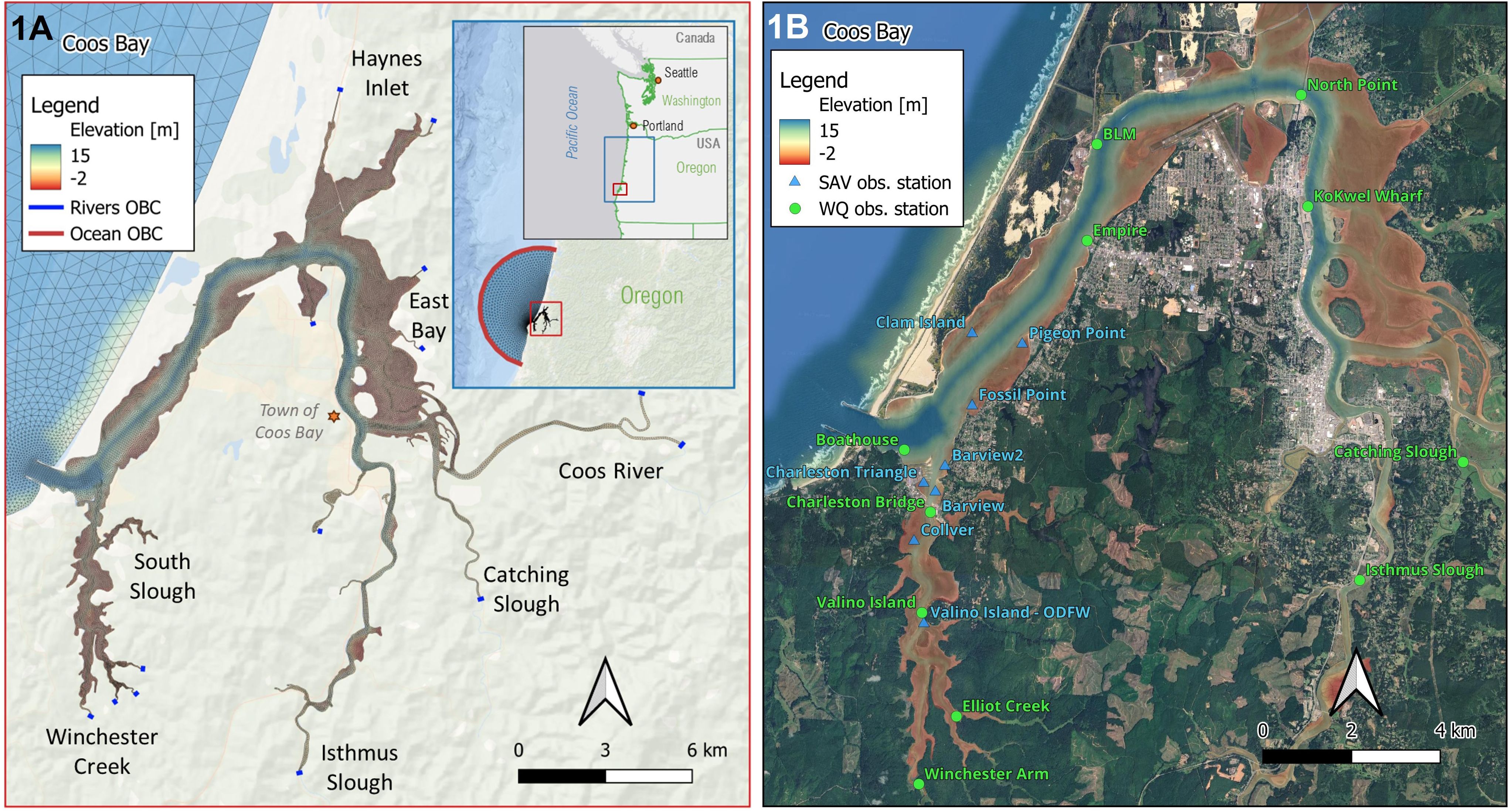
Figure 1. Maps of the Coos Bay estuary, Oregon, U.S. showing the grid, open ocean boundary, and river input locations of the model (A) and the observation stations used in model calibration (B) for water quality (green circles) and submerged aquatic vegetation (SAV, i.e. eelgrass; blue triangles).

Environmental and biological monitoring associated with SSNERR has been ongoing in Coos Bay since the early 2000s, although most monitoring has occurred within the smaller, southern arm (Winchester Creek). Periodic monitoring of water quality and eelgrass has occurred in the main, northern arm supported by SSNERR and other partners, including local tribes (Confederated Tribes of Coos, Lower Umpqua and Siuslaw Indians and Coquille Indian Tribe) and state and federal agencies [Oregon Department of Fish and Wildlife (ODFW), Oregon Department of Environmental Quality (ODEQ), and U.S. Environmental Protection Agency (EPA)]. An existing hydrodynamic model of Coos Bay was established for the year 2014 (Conroy et al., 2020; Eidam et al., 2020). Among others, these prior data collection and modeling efforts provided the basis for development of a biophysical model of the estuary.

2.2 Biophysical model framework

The hydrodynamic model of Coos Bay (Conroy et al., 2020) simulates hydrodynamics using a Finite Volume Coastal Ocean Model (FVCOM) that solves the three-dimensional equations of continuity and momentum on an unstructured grid (Chen et al., 2003). The FVCOM framework allows for wetting and drying of grid cells to accommodate water-level fluctuations associated with tides. The model boundary conditions include river and stream inflows at 14 locations and tidal forcing and salinity at the open boundary with the coastal ocean. For this study, we modified the original model grid of Coos Bay described by Conroy et al. (2020) into a coarser grid to significantly reduce computation time, while still achieving a similar level of performance in simulating salinity. Our modifications to the original hydrodynamic model included reducing the number of model nodes by 75%, reducing the number of model layers from 20 to 10 layers, and smoothing the model bathymetry. Model input forcing and initial conditions such as water surface elevation, temperature and salinity at the boundary, and meteorological forcings (i.e. heat flux and wind) were implemented in the same fashion as Conroy et al. (2020).

We then established the biogeochemical model for Coos Bay including eelgrass using FVCOM-ICM (Kim and Khangaonkar, 2012), which conducts water quality and biological calculations based on CE-QUAL-ICM kinetic formulation (Cerco and Cole, 1995). FVCOM-ICM uses previously produced hydrodynamic solutions over the same FVCOM modeling framework. The biogeochemical model simulates processes including phytoplankton production, nutrient consumption, mineralization, and decay and settling of organic matter and ultimately computes resulting DO and pH levels (Supplementary Figure 1). The eelgrass submodel is divided into two compartments, above and belowground, which have their own kinetics that depend on light availability, nutrient uptake, and mortality. The eelgrass submodel has previously been implemented, tested, and validated for Zostera marina in Puget Sound, Washington (Khangaonkar et al., 2021a).

2.3 Model inputs, simulation, and calibration

The hydrodynamic model domain includes 14 river input locations and flow rates from Y2014 were utilized for each (Conroy et al., 2020). For the biogeochemical model, water quality data were needed for each of the river input locations. Continuous sampling for temperature and nutrients in 2014 was only available for Winchester Creek, which is a location of SSNERR’s System-Wide Monitoring Program (SWMP; downloaded from https://cdmo.baruch.sc.edu/). The location of the Winchester SWMP station (code: ‘soswi’) is tidally influenced, so 2014 monitoring data were filtered for low salinity (< 6 ppt) to create an annual timeseries approximating the freshwater conditions at that site. For the remainder of the river input locations, we performed a synthesis combining the 2012–2016 Winchester SWMP data and all other water quality monitoring data available from ODEQ for rivers and streams in the Coos Bay watershed (HUC 17100304) from 1999-2022 (downloaded from www.oregon.gov/deq/wq/pages/wqdata.aspx). Figure 1 provides a site map of Coos Bay estuary, showing the model grid, open ocean boundary, and river input locations of the model and water quality observation stations used in the model calibration.

In limited cases where salinity or conductivity data were available alongside temperature or nutrient data, the ODEQ data was filtered by low salinity (approximately < 6 ppt). In most cases, however, salinity information was not available, therefore the ODEQ data were also qualitatively filtered for locations that should have primarily freshwater influence based on their location in the watershed (Supplementary Figure 2). From this dataset, we calculated monthly averages for temperature, pH, alkalinity, nutrients (nitrate+nitrite, ammonia, and phosphate), and organic carbon, which were used as inputs for the other 13 rivers in the model.

Temperature and salinity profiles for the ocean were obtained from the LiveOcean model (MacCready et al., 2021) over the continental shelf and were interpolated to the model’s boundary (Conroy et al., 2020). Ocean boundary values for most other water quality variables were set based on available climatological data from a combination of World Ocean Atlas and the Canadian Department of Fisheries and Oceans monitoring database (Boyer et al., 2018; Gregory, 2004) with the exception of DO, nitrate+nitrite, total alkalinity, and dissolved inorganic carbon. Based on observations from multiple cruises over the PNW continental shelf, these variables are strongly correlated to salinity (Davis et al., 2014; Siedlecki et al., 2015) and regression equations have been developed to describe those relationships (personal communication from Ryan McCabe and Parker MacCready, University of Washington). These regressions have been used extensively in the models of the Salish Sea and are a significant improvement over fixed conditions (Khangaonkar et al., 2019; 2021a).

Eelgrass monitoring (percent cover and shoot density) is routinely conducted at several sites in South Slough, associated with SWMP biological monitoring (Moore, 2013). Additional eelgrass datasets, including percent cover, shoot density, and biomass in Coos Bay were available from published studies (Hessing-Lewis et al., 2011; Hayduk et al., 2019; Magel, 2020; Magel et al., 2023) and from the Oregon Department of Fish and Wildlife’s Shellfish and Estuarine Assessment of Coastal Oregon monitoring program. Values of biomass (grams dry weight) were converted into grams of carbon by assuming approximately 36% of total dry weight is carbon, based on prior carbon content analyses for Zostera marina (Duarte, 1990; Fourqurean et al., 1997). These data, spanning 2008-2019, were used as initial condition biomass and to calibrate/validate performance of the eelgrass submodel. Algal (diatoms and dinoflagellates) and eelgrass submodel parameters were taken from Cerco and Cole (1993) and Khangaonkar et al. (2021a).

Overall model performance for water quality was evaluated using error statistics such as absolute mean error (AME) or mean error (ME) to assess bias and root-mean-square error (RMSE). The AME and RMSE of timeseries with N elements are defined as follows:

$$AME=\frac{1}{N} \left|(X_{mdl}-X_{obs})\right|$$

$$RMSE = \sqrt{\frac{\Sigma {(X_{mdl}-X_{obs})}^2}{N}}$$

where $X_{mdl}$ and $X_{obs}$ are the values from the model and observations, respectively. To assess model skill, we computed the Willmott Skill Score (SS) (Willmott, 1982), defined as:

$$SS= 1-\frac{\mathit{\text{Σ}}{(X_{mdl}-X_{obs})}^2}{\mathit{\text{Σ}}{\left(\left|X_{mdl}-{\overline{X}}_{obs}\right|+\left|X_{obs}-{\overline{X}}_{obs}\right|\right)}^2}$$

where an overbar represents a time average. The SS is a measure of the level of agreement between the observed and modeled values; a value of 1 indicates perfect agreement and a value of 0 indicates no agreement.

The hydrodynamic, water quality, and eelgrass model calibrations involved an iterative process of adjustment and evaluation of the model properties and parameters. The calibration process was performed initially for the hydrodynamic model, and subsequently for the water quality model and eelgrass submodel for Y2014. This sequential approach ensures hydrodynamic stability before the water quality and eelgrass calibrations. For the hydrodynamic model, we adjusted the model’s grid properties (i.e. grid extent and sizes) and number of layers to minimize the RMSE and maximize the SS. Water quality model calibration of the Coos Bay model was conducted using timeseries data from 11 water-quality stations with sensors located approximately 0.5–1 m above the bottom maintained by SSNERR, Confederated Tribes of the Coos, Lower Umpqua and Siuslaw Indians, and Coquille Indian Tribe (Figure 1B). For calibration of the eelgrass submodel, we adjusted the eelgrass growth rate parameter and compared the simulated biomass to (limited) observations from Y2014 and our synthesis of observations between 2008 and 2019. Because eelgrass monitoring was not collected using continuous timeseries and the general scarcity of biomass data, performance of the eelgrass model was evaluated by visually comparing the modeled timeseries to box plots of eelgrass biomass data from general sites and timepoints. This iterative, data-driven calibration approach ensured that each model component was tuned to reflect observed conditions as closely as possible, thereby increasing confidence in the model’s predictive capability.

2.4 Eelgrass scenario analyses

Using the validated biophysical model, we ran three eelgrass extent scenarios: zero eelgrass, current extent, and maximum observed extent. These captured a range of eelgrass abundance conditions in Coos Bay and allowed for a screening-level assessment of the effect of eelgrass abundance on OAH conditions. The “no eelgrass” scenario represented complete loss of eelgrass from the entire estuary. Eelgrass extents for the other two modeled scenarios were determined from previous mapping efforts performed in 1978, 2005, and 2016 (synthesized in Sherman and DeBruyckere (2018) and downloaded from www.pacificfishhabitat.org/data/west-coast-usa-eelgrass-habitat/). The “current extent” scenario used a modified version of the 2016 extent layer, described in more detail below. The “maximum observed extent” scenario was a combination of the 1978, 2005, and our modified 2016 maps.

The 2016 survey, performed by Quantum Spatial Inc. (Corvallis, OR) under contract to Friends of South Slough, used 4-band multispectral orthoimagery to identify eelgrass habitats in Coos Bay in July 2016. Training and validation data were also collected in 2016 using boat-based single beam sonar transects. The final map of Coos Bay eelgrass was classified into low, medium, and high confidence areas. For our “current extent” scenario, we selected both medium and high confidence areas which included those that were spectrally or contextually positive for eelgrass (medium confidence), spectrally and contextually positive (high confidence), and those that were hand digitized (high confidence). While Sherman and DeBruyckere (2018) only included high confidence areas for the 2016 layer, we also included the medium confidence areas because other field surveys conducted in 2016 found eelgrass in at least some of the medium confidence areas (Magel et al., 2023). The 2016 spatial data files containing both medium and high confidence areas were obtained directly from SSNERR and were converted from raster format to polygons as eelgrass area coverage using GIS tools. Those polygons were used to create the initial conditions that represent the state of eelgrass in the model domain (as a node) at the start of simulation (Figure 2).

Figure 2

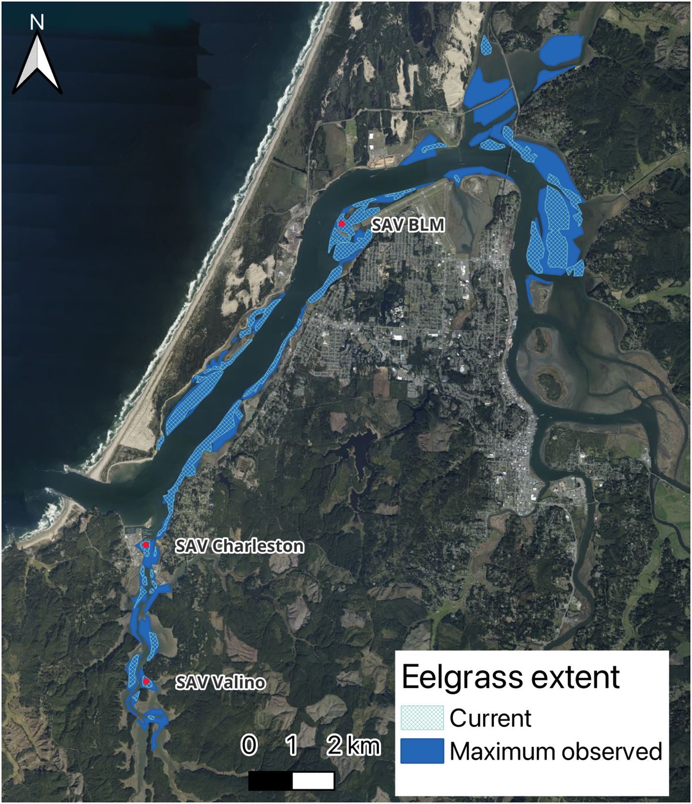
Figure 2. Model coverage of eelgrass used to simulate the “current extent” (hatched light blue area) and “maximum observed extent” (solid dark blue area) scenarios for Coos Bay, Oregon. Red dots indicate locations used to visualize results of the modeled eelgrass scenarios.

For each scenario, the biogeochemical model simulated water quality and eelgrass dynamics from January through December Y2014. The results of the three scenarios were compared to evaluate the influence of Coos Bay eelgrass on OAH-dependent water quality, including DO, pH, and the calcium carbonate saturation state for aragonite (Ω). The latter parameter was calculated using the program called ‘CO2SYS’ (Orr et al., 2018), based on input parameters such as total alkalinity, total inorganic carbon or pH, temperature, salinity, and concentrations of phosphate from the model results. CO2SYS employs various equilibrium constants for the dissociation of carbonic acid and other species to determine the concentrations of carbonate species in the water. The aragonite saturation state (Ω) is then calculated using the formula:

$${\Omega }_{aragonite}=\frac{[C{a}^{2+}]·[C{O}_3^{2-}]}{K_{sp}}$$

, where $[C{a}^{2+}]$ is the calcium ion concentration, $[C{O}_3^{2-}]$ is the carbonate ion concentration, and $K_{sp}$ is the solubility product of aragonite. The program outputs aragonite saturation state along with other carbonate system parameters at the specified conditions. Seawater with low pH also has a low aragonite saturation state. Aragonite is the least stable form of calcium carbonate, formed by many shell-building organisms, and its saturation state indicates whether aragonite tends to precipitate (Ω > 1) or dissolve (Ω < 1). Ω levels below 1 are of concern as this indicates conditions unsuitable for calcifying organisms to build shells (Doney et al., 2009).

The water quality results were analyzed in several ways. First, timeseries and monthly boxplots of DO and pH were visually compared between the three scenarios. Results are presented for three sites located within eelgrass beds that are spatially distributed around the estuary - BLM in the northern, main arm of Coos River, Charleston near the mouth of the estuary, and Valino in the southern, Winchester arm. Next, we calculated exceedances of the following biologically relevant thresholds: DO < 6.5 mg/L following Oregon’s coastal water quality standard based on salmonid physiological requirements (Brown and Nelson, 2015), pH < 7.8 based on juvenile Olympia oyster performance (Hettinger et al., 2012), and aragonite saturation state (Ω) < 1 representing a corrosive condition that favors dissolution of calcium carbonate shells and skeletons (Doney et al., 2009). We summarized threshold exceedances by calculating the total volume-hour (m³-hr) of the model domain below each biological threshold. The total volume-hour was calculated for each node and layer in the model. The total volume for each node/layer below the threshold was integrated over the water column and time for the modeled year (Y2014). Furthermore, to better understand the relative difference among eelgrass extent scenarios, we calculated the fraction change in volume-hour for each parameter and each model node between the scenarios. The difference in fraction volume-hour for DO, pH, and aragonite saturation state were visualized as contoured maps.

3 Results

3.1 Model input synthesis

Synthesis of the ODEQ and SSNERR water quality data resulted in a dataset of 24 unique locations with freshwater quality information from the Coos Bay watershed (Supplementary Figure 2A). While spatially distributed across much of the watershed (9 of the 14 subwatersheds in the model), most of the monitoring was temporally limited - often encompassing only one grab sample and up to a week of continuous data. In addition, the available data was heavily weighted towards summer and fall (92% of the 34,678 observations). Given these limitations, we were not able to produce unique timeseries for each of the model’s 14 river input locations. Instead, we calculated monthly averages that were applied to all river input locations, except Winchester Creek (Supplementary Table 1). For Winchester Creek, 2014 monitoring data from the SSNERR SWMP station were used, which included continuous water quality measurements (temperature, salinity) and monthly nutrient grab samples.

Between 2008 and 2019, observations of eelgrass AG biomass were made at 15 sites in Coos Bay (Supplementary Figure 2B). While there was variability across sites and years, average aboveground (AG) biomass across those observations was 96.4 grams dry weight per 0.25 m² (Supplementary Figure 3A). Observations of belowground (BG) biomass were limited to only two sites between 2016 and 2019. From those limited samples, average BG biomass was 198.0 grams dry weight per 0.25 m² (Supplementary Figure 3B).

3.2 Model calibration

First, the hydrodynamic model was calibrated by adjusting the model’s grid properties (i.e. grid extent and sizes) and number of layers to minimize the RMSE, maximize the SS, and reduce computational time. Calibration metrics for temperature and salinity are presented in Supplementary Table 2. The RMSE for temperature ranged from 1.59°C to 3.68°C, with the highest errors occurring at stations along the main channel of Coos Bay. Model-observation errors for temperature were particularly pronounced during the summer (Figure 3; Supplementary Figures 4-5), likely because the estuary was more stratified than the model represented. The Skill Score (SS) for temperature was generally high, ranging from 0.57 to 0.98, indicating that despite some errors, the model performed reasonably well overall. Notably, Catching Slough and Coos River stations exhibited the best performance with SS values close to 1, likely because these stations were located closest to the model boundary. For salinity, the RMSE values ranged from 2.9 ppt to 10.7 ppt, with an outlier at Catching Slough where the RMSE reaches 40.71 ppt, possibly due to sensor errors during the summer period. The SS for salinity varied more widely, from 0.14 at Catching Slough to 0.87 at North Point. Stations such as BLM, North Point, and Coos River had good performance with SS values > 0.75. In contrast, stations like Elliot, Isthmus Slough, and Winchester had higher RMSE values (> 5) and lower SS values (< 0.6), indicating that the model underpredicted the high variability of salinity during the summer months (Figure 3; Supplementary Figures 4-5).

Figure 3

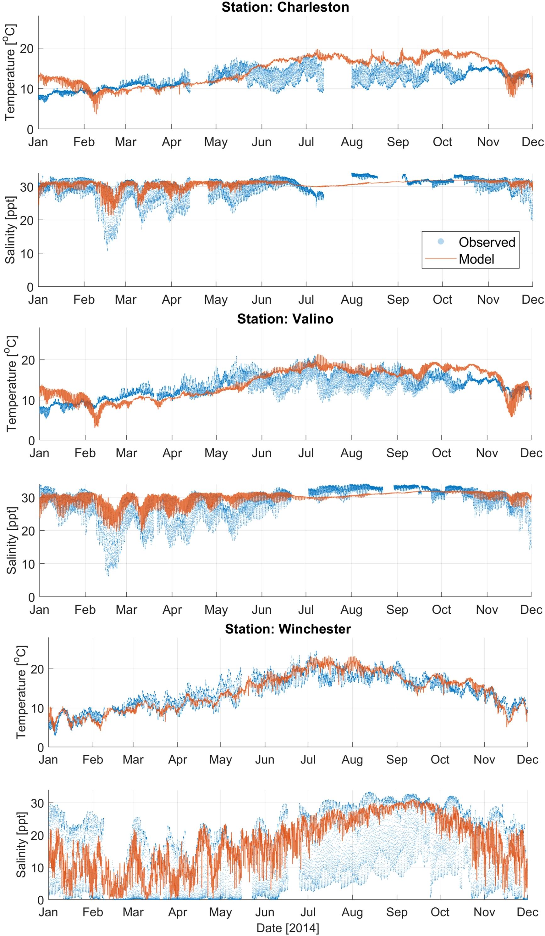
Figure 3. Comparison of modeled results (orange line) and observations (blue dots) for temperature and salinity at Charleston, Valino, and Winchester water quality stations (Figure 1B). Temperature and salinity results from additional stations are shown in Supplementary Figures 4, 5.

Despite using a significantly coarser grid (300 m versus 15 m) and fewer vertical layers in the hydrodynamic model, the current study achieved computational efficiency with only moderate accuracy trade-offs compared to Conroy et al. (2020). The current model simulated 264% faster (20 hours versus 264 hours) for a one-year simulation on University of Washington’s high performance computing system, HYAK, using 10 nodes (400 cores). While the salinity RMSE increased by 9-32% [2.9-10.7 ppt compared to 2.1-3.8 ppt of Conroy et al. (2020)], higher errors were primarily concentrated in the upper estuary region away from the eelgrass sites of interest. Normalized RMSE were calculated using the observed range values to justify that the model skill obtained was sufficient for simulating water quality in Coos Bay. For temperature, NRMSE ranged from 7–54% (mean 20.8%) of the observed mean temperature range 15.9°C in Coos Bay (RMSE values: 1.59–3.68°C), while RMSE for salinity (2.9–10.7 ppt) was 9–32% (mean 19.0%) of the observed mean salinity range (30.9 ppt). These normalized metrics fall within 20% of the relative RMSE, which is considered satisfactory performance criteria for hydrodynamic modeling (Moriasi et al., 2015). The model adequately captured the key physical processes driving water quality in Coos Bay, including tidal mixing and seasonal temperature patterns. The temperature RMSE (≤3.68°C) is smaller than seasonal variability (Δ~10°C), which can drive biogeochemical rates (Marin Jarrin et al., 2022). We also observed that salinity errors (≤10.7 ppt) primarily occur near the river boundaries, while main-channel performance (SS >0.75) ensures reliable transport physics for nutrient and DO dynamics.

Second, water quality calibration was performed by adjusting key biogeochemical parameters, including phytoplankton growth and mortality rates, nutrient uptake kinetics, and settling velocities. Where possible, we adopted parameter values from the previously calibrated Salish Sea Model (Khangaonkar et al., 2021a) to ensure consistency and leverage established best practices. For each parameter, we manually specified and tested adjustment ranges, using RMSE and SS as primary performance metrics for water quality variables such as DO, nutrients, and chlorophyll-a. Calibration metrics for DO and pH are presented in Supplementary Table 3. The RMSE values for DO varied from 0.89 mg/L to 4.36 mg/L, with the highest errors observed at the BLM station. Unrealistic observed DO values at BLM station might be due to instrument malfunction. The Skill Score (SS) for DO ranged from 0.43 to 0.90, with Coos River and Catching Slough stations showing the best performance. The Mean Error (ME > or< 1 mg/L) values indicated that the model tended to underpredict/overpredict DO at several stations, such as Boathouse at -1.44 mg/L, while overpredicting at Isthmus Slough at 1.45 mg/L. On average, the RMSE value for DO is 1.4 mg/L. The RMSE value for pH ranged from 0.15 to 0.77, with the highest error at Winchester and the lowest at Boathouse. The SS value for pH ranged from 0.35 to 0.65. The average ME value for all the stations is 0.3 whereas the RMSE is 0.4. Overall, this result indicates that the model overpredicted pH especially at stations that are upstream close to the river mouths such as Winchester, Isthmus Slough, Catching Slough, and Coos River.

Calibration metrics for nitrate, ammonium, and chlorophyll-a (chl-a) for Coos Bay are presented in Supplementary Table 4. For nitrate, the Valino station showed relatively low near zero ME and RMSE values. However, the SS for this station was relatively low at 0.53. Charleston and Winchester stations had slightly higher SS values > 0.6, with Winchester showing a negative ME, indicating a tendency to underpredict nitrate levels. The ammonium metrics were generally better, with higher SS values (> 0.6) across the stations. The average ME and RMSE were relatively low at 0 mg/L and 0.02 mg/L, respectively. Chl-a metrics, however, indicated higher errors, especially at Valino and Charleston, where RMSE values were significantly higher. The SS for chl-a were also lower compared to nitrate and ammonium. The Boathouse station performed better for chl-a with moderate RMSE and SS values. Figures 4–6 show the timeseries plots for DO, pH, chl-a, nitrate and ammonium for Y2014 observations and model results at 3 selected stations (results from additional stations are shown in Supplementary Figures 6-13). Despite having a moderate ability to predict water quality conditions (DO, pH, nutrients, and chl-a), the model reproduced observed average conditions and variability.

Figure 4

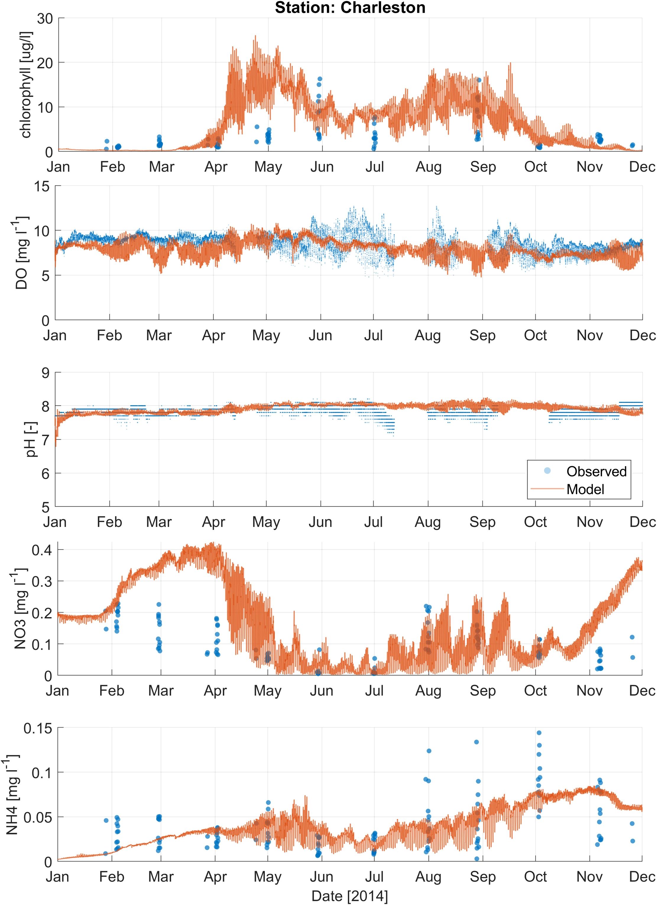
Figure 4. Comparison of modeled results (orange line) and observations (blue dots) for water quality parameters, including chlorophyll-a, dissolved oxygen (DO), pH, nitrate (NO₃^-), and ammonium (NH₄⁺), at the Charleston station (Figure 1B).

Figure 5

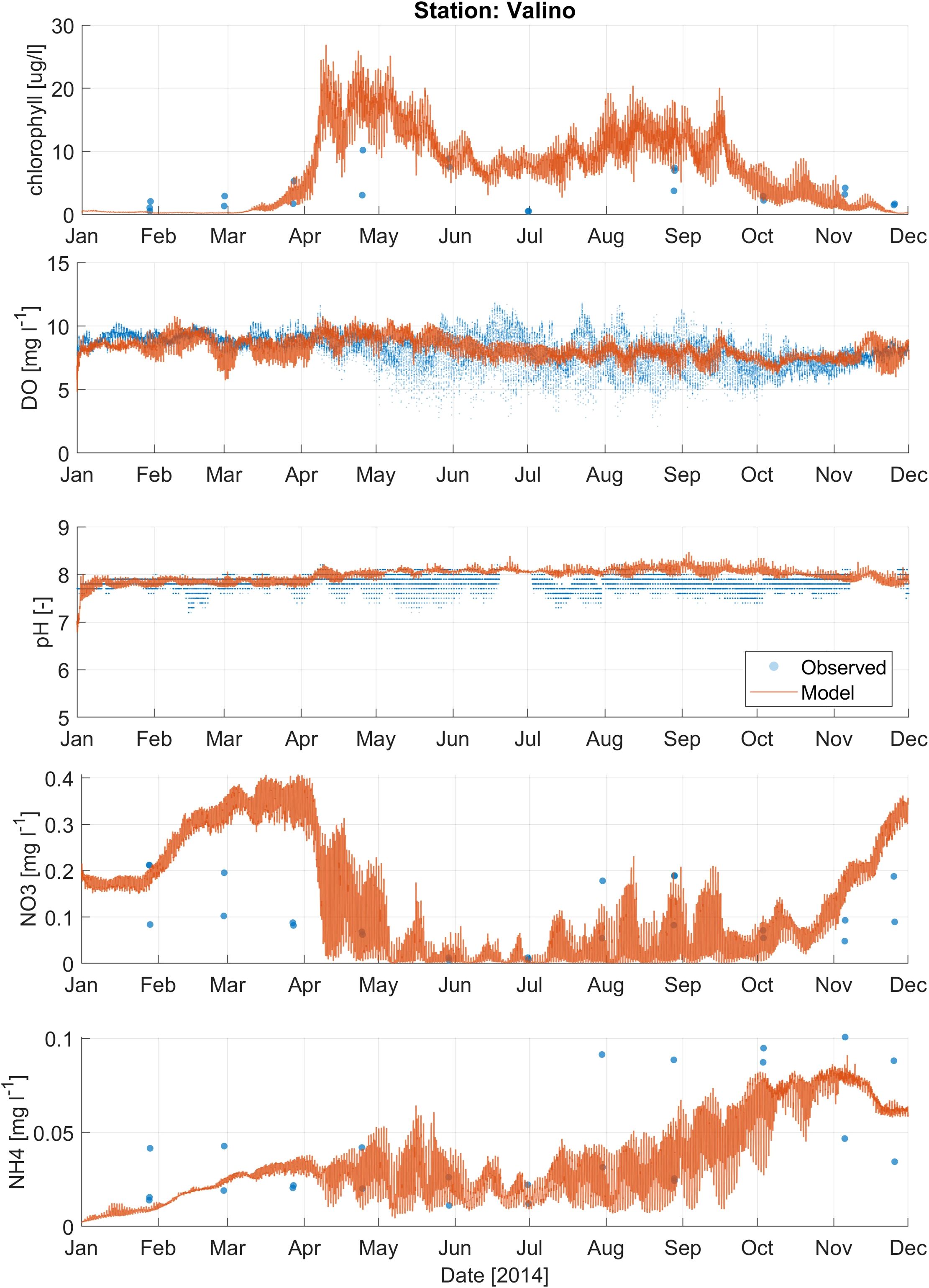
Figure 5. Comparison of modeled results (orange line) and observations (blue dots) for water quality parameters, including chlorophyll-a, dissolved oxygen (DO), pH, nitrate (NO₃^-), and ammonium (NH₄⁺), at the Valino station (Figure 1B).

Figure 6

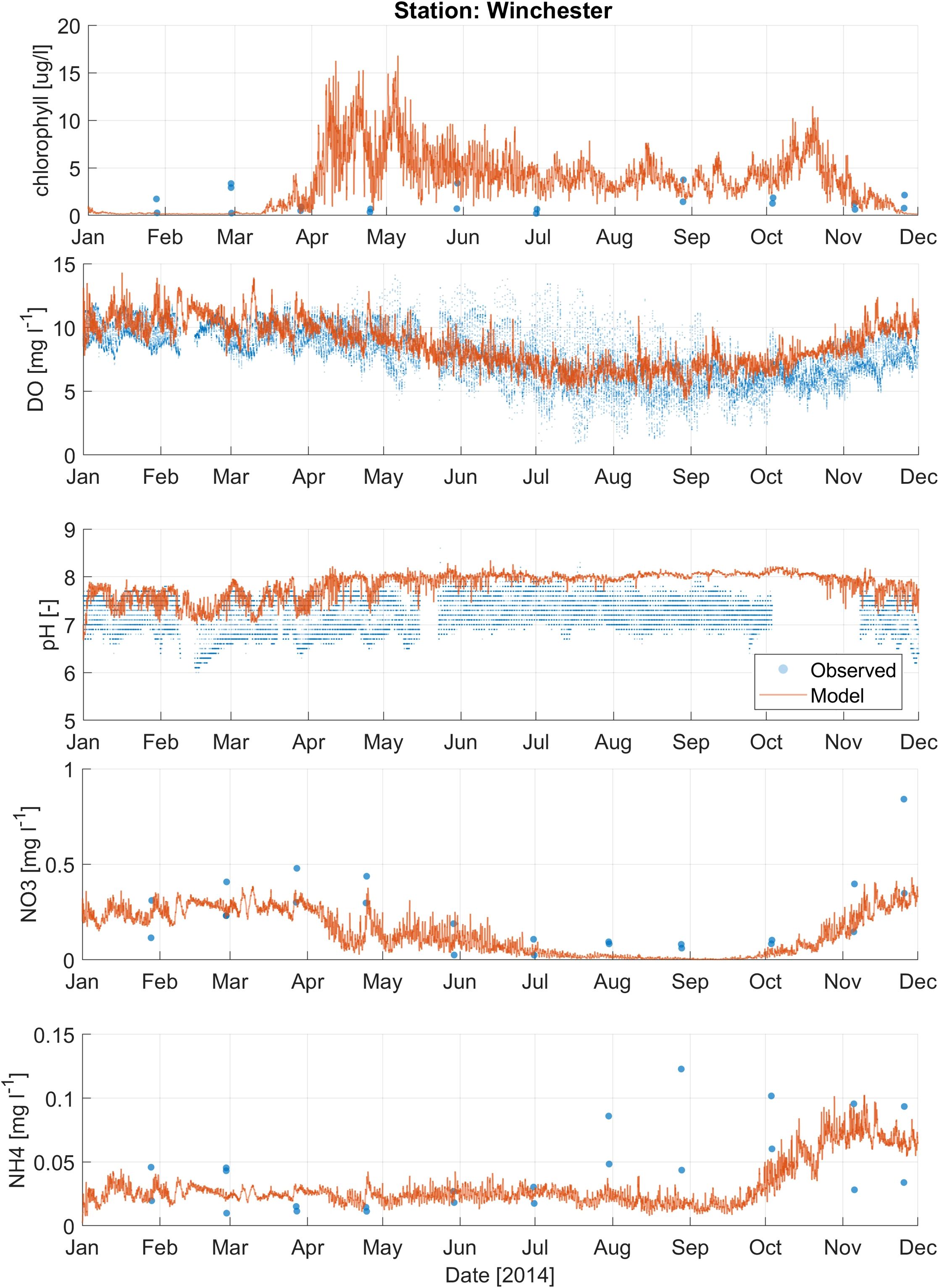
Figure 6. Comparison of modeled results (orange line) and observations (blue dots) for water quality parameters, including chlorophyll-a, dissolved oxygen (DO), pH, nitrate (NO₃^-), and ammonium (NH₄⁺), at the Winchester station (Figure 1B).

Last, we calibrated the eelgrass submodel. Due to data availability limitations from Y2014, validation of eelgrass model was primarily qualitative and was evaluated using results from the current extent scenario at 7 locations in Coos Bay (Figure 1B). Due to limitations of the number of eelgrass biomass samples and high variability of observed biomass values, we used the median to compare with simulated eelgrass biomass (Figure 7). We adjusted the eelgrass growth rate parameter and compared the simulated biomass to observations. The range of simulated AG biomass in Coos Bay was between 45.1-48.7 gC/m² during summer time, which was similar to the range of observed AG biomass with a median of 49.1 gC/m². Only two stations had BG eelgrass biomass data for comparison (Figure 7). Observed BG biomass at those two stations had a median of between 16.3 to 20.7 gC/m² in July, which was close to the predicted BG eelgrass biomass from model results of 15.7 gC/m². The model provided a reasonable approximation of both AG and BG eelgrass biomass where observations were available.

Figure 7

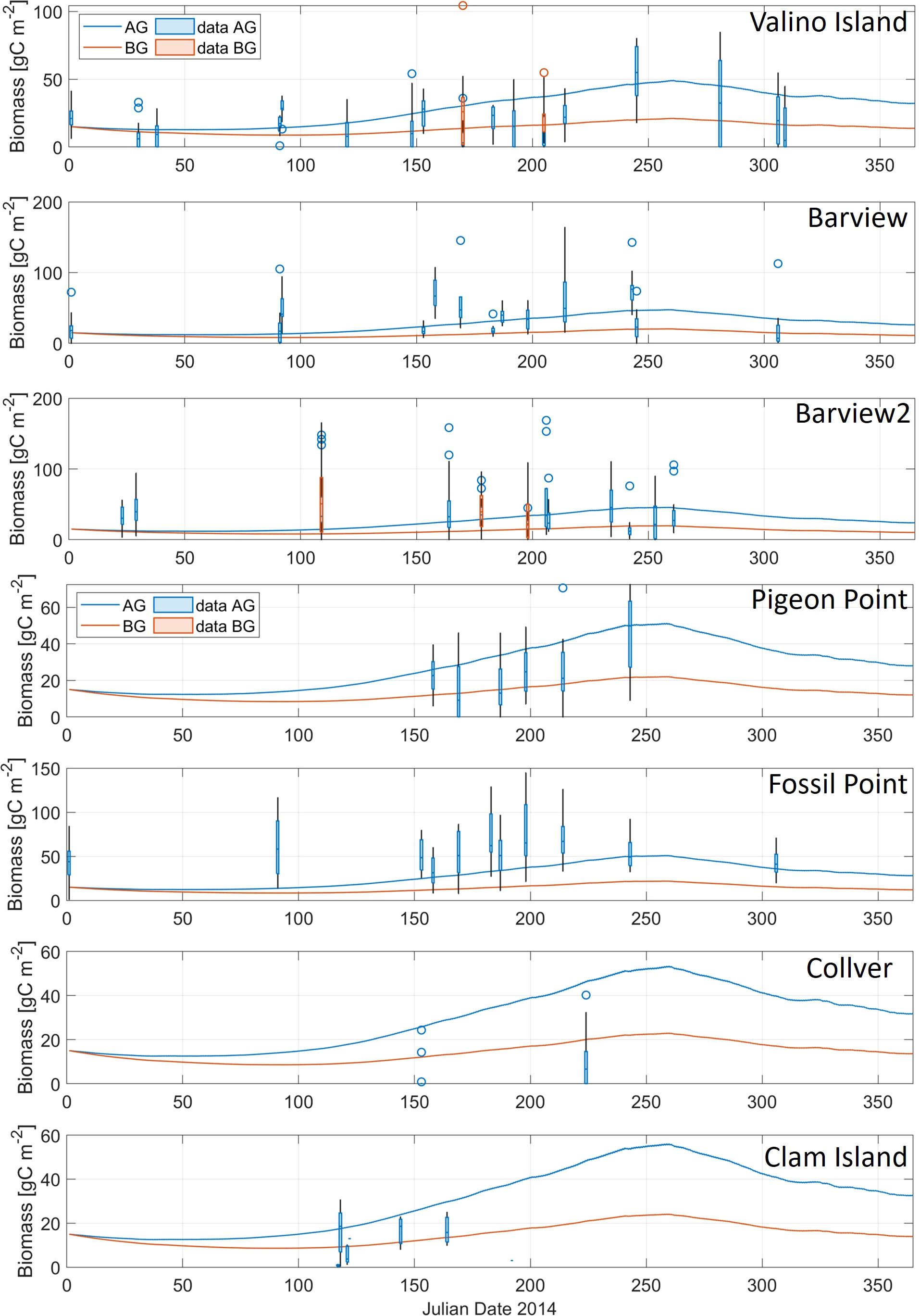
Figure 7. Comparison of model result (lines) and observations (box and whiskers) for eelgrass biomass, including above ground (AG; blue) and belowground (BG; red), at seven eelgrass sites in Coos Bay, Oregon (Figure 1B). Note differences in y-axes between sites.

3.3 Scenario comparisons

We compared the spatial distribution of AG and BG eelgrass biomass in September 2014 between the current extent and maximum observed extent scenarios (Supplementary Figure 14). The lower, marine-dominated area of Coos Bay had higher AG and BG eelgrass biomass. For instance, at Barview station, AG eelgrass biomass was as high as 50 gC/m², while in the upriver section of Coos River, AG biomass was approximately 29 gC/m². Comparing the two scenarios, there was little difference in AG and BG eelgrass biomass, except for the wider spatial coverage of eelgrass used in the maximum extent scenario (Figure 2).

While the model without eelgrass adequately matched the average DO and pH conditions, it did not capture the high variability and extremes present in the observations. Including eelgrass in the model via scenarios of current extent and maximum observed extent resulted in greater variability and extremes in pH and DO compared to the model without eelgrass (Figures 8, 9). Model results from the two eelgrass scenarios more closely matched the high temporal variability present in the observations (e.g., Figures 4-6).

Figure 8

Figure 8. Timeseries of modeled dissolved oxygen (mg/L) in the bottom layer for three eelgrass scenarios [no eelgrass (yellow), current extent (light blue), and maximum observed extent (dark blue)] at three sites in Coos Bay, Oregon (Figure 2).

Figure 9

Figure 9. Timeseries of modeled pH in the bottom layer for three eelgrass scenarios [no eelgrass (yellow), current extent (light blue), and maximum observed extent (dark blue)] at three sites in Coos Bay, Oregon (Figure 2).

Comparing the scenario results for DO at three sites within eelgrass beds, changes in the average DO concentration were limited but there was an increase in the variability and extremes (Table 1; Figure 8). In general, the two models with eelgrass had higher highs and lower lows for DO but differences among scenarios were site specific. There was a large difference in DO among the scenarios at BLM (variability increased dramatically), a small difference at Valino, and almost no discernible difference at Charleston. Nearly all the change among scenarios occurred between the no eelgrass and current extent scenarios and very little additional change occurred between the current extent and maximum observed extent scenarios. Differences among scenarios were also seasonally specific - changes at BLM and Valino were most pronounced during summer and fall (approximately May through October).

Table 1

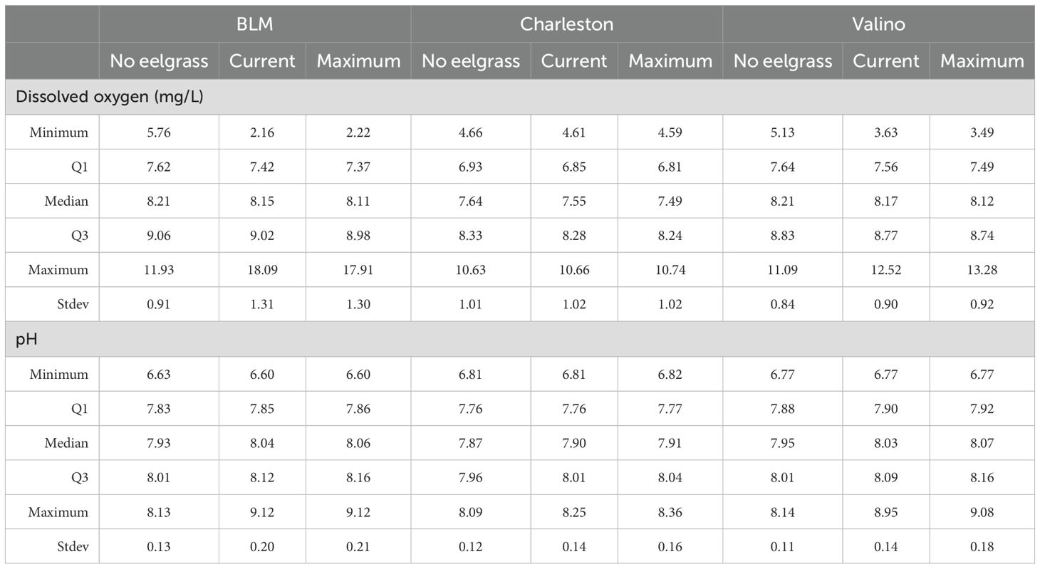
Table 1. Summary of July 2014 modeled dissolved oxygen and pH conditions [minimum, first quartile (Q1), median, third quartile (Q3), maximum, and standard deviation (stdev)] from the bottom layer for the three scenarios (no eelgrass, current extent, and maximum observed extent) at three locations in Coos Bay, Oregon (Figure 2).

Compared to DO, pH differences across modeled scenarios were larger at all three sites and scenarios with eelgrass present had both higher average pH and larger variability (Table 1; Figure 9). pH in the eelgrass scenarios had higher highs, but in most cases did not have lower lows, which were observed in the DO results. Similar to DO, differences among scenarios were seasonally specific and were most pronounced during summer and fall at all three sites. The largest changes occurred between the no eelgrass and current extent scenarios at all three sites, but Charleston and Valino also had a notable increase in pH in the maximum observed extent scenario.

While not the primary focus of our scenario analysis, nutrient and chlorophyll results were also compared across scenarios. Nitrate concentrations and dynamics were similar across the three modeled scenarios (Supplementary Figure 15). Ammonium concentration was lowest in the current extent scenario at all three sites and diverged most from the other two scenarios in the late summer and early fall (Supplementary Figure 16). The highest ammonium concentrations at each site tended to occur in the late summer and fall, particularly in the maximum observed extent scenario. BLM had higher concentrations and variability in ammonium compared to the other two sites. Chl-a dynamics were fairly similar across the three sites, with two peaks observed - a higher peak in spring and a lower peak in late summer (Supplementary Figure 17). The current extent scenario had higher maximum chl-a across the timeseries compared to the other two scenarios at all three sites.

Using biologically relevant thresholds for DO (6.5 mg/L), pH (7.8), and aragonite saturation state (1), we calculated a volumetric-temporal metric (volume-hours) to capture the amount of Coos Bay below those thresholds in the Y2014 model results. Synthesizing across the volume and temporal results, the occurrence of DO below the threshold was most common and pH below the threshold was least common (Table 2). The magnitude of pH and aragonite saturation state exceedances decreased in the current extent and maximum observed extent scenarios relative to the no eelgrass scenario, whereas DO exceedances increased slightly. Using the volume-hour calculation of threshold exceedances, we also performed a hot spot analysis to identify where these OAH conditions were mitigated or enhanced between the three scenarios. For DO, there was a 0.6% increase in volume-hour below 6.5 mg/L between the no eelgrass and current extent scenarios and an additional 0.3% increase in the maximum observed extent scenario (Table 2). Within the slight overall increases in % volume-hour DO, some areas increased while others decreased (Figure 10). Increases in the threshold exceedance mostly occurred in the upper reaches of the estuary and nearshore areas (both Coos River and Winchester Creek arms), but decreases were observed on some of the large intertidal flats of the northern arm (e.g., Haynes Inlet and East Bay) and in some shallow areas fringing the main channel at the center of the bay (e.g., Empire, Fossil Point) (see Figure 1 referenced locations). Decreases in harmful DO conditions primarily occurred in areas of added eelgrass to the model – indicated by the hatched area in Figure 10. For pH, there was a 7.6% reduction in the total volume-hour below 7.8 pH between the no eelgrass and current extent scenarios and an additional 5.3% reduction in the maximum observed extent scenario (Table 2). The largest reductions in % volume-hour pH primarily occurred in shallow areas fringing the main channel in the center of the bay (current extent scenario) and in the large intertidal flats of Haynes Inlet and Easy Bay (maximum observed extent scenario) (Figure 11). The largest reductions in harmful pH conditions occurred in and around the areas of added eelgrass – indicated by the hatched areas in Figure 11. Smaller reductions in % volume-hour pH were distributed across the estuary and no areas of increase were identified. For aragonite saturation state (Ω), there was a 2.6% reduction in volume-hour below 1 between the no eelgrass and current extent scenarios and an additional 1.9% reduction in the maximum observed extent scenario (Table 2). These reductions in % volume-hour Ω primarily occurred near Airport Flat, Haynes Inlet, and Easy Bay (current extent scenario) and in the upper reaches of South Slough and Haynes Inlet (maximum observed extent scenario) (Figure 12). Changes in volume-hour Ω were generally small and appeared less closely tied to the areas of added eelgrass (hatched areas of Figure 12) compared to DO and pH. Smaller reductions in % volume-hour Ω were distributed across the estuary and no areas of increase were identified.

Table 2

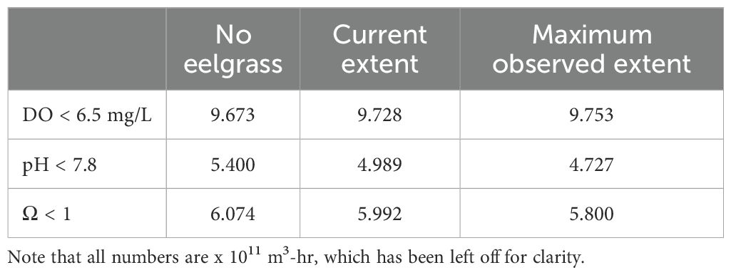
Table 2. Summary of estuary wide calculation for volume-hours (m³-hr) dissolved oxygen (DO), pH, and calcium carbonate saturation state for aragonite (Ω) exceeding biologically relevant thresholds for the three scenarios (no eelgrass, current extent, and maximum observed extent).

Figure 10

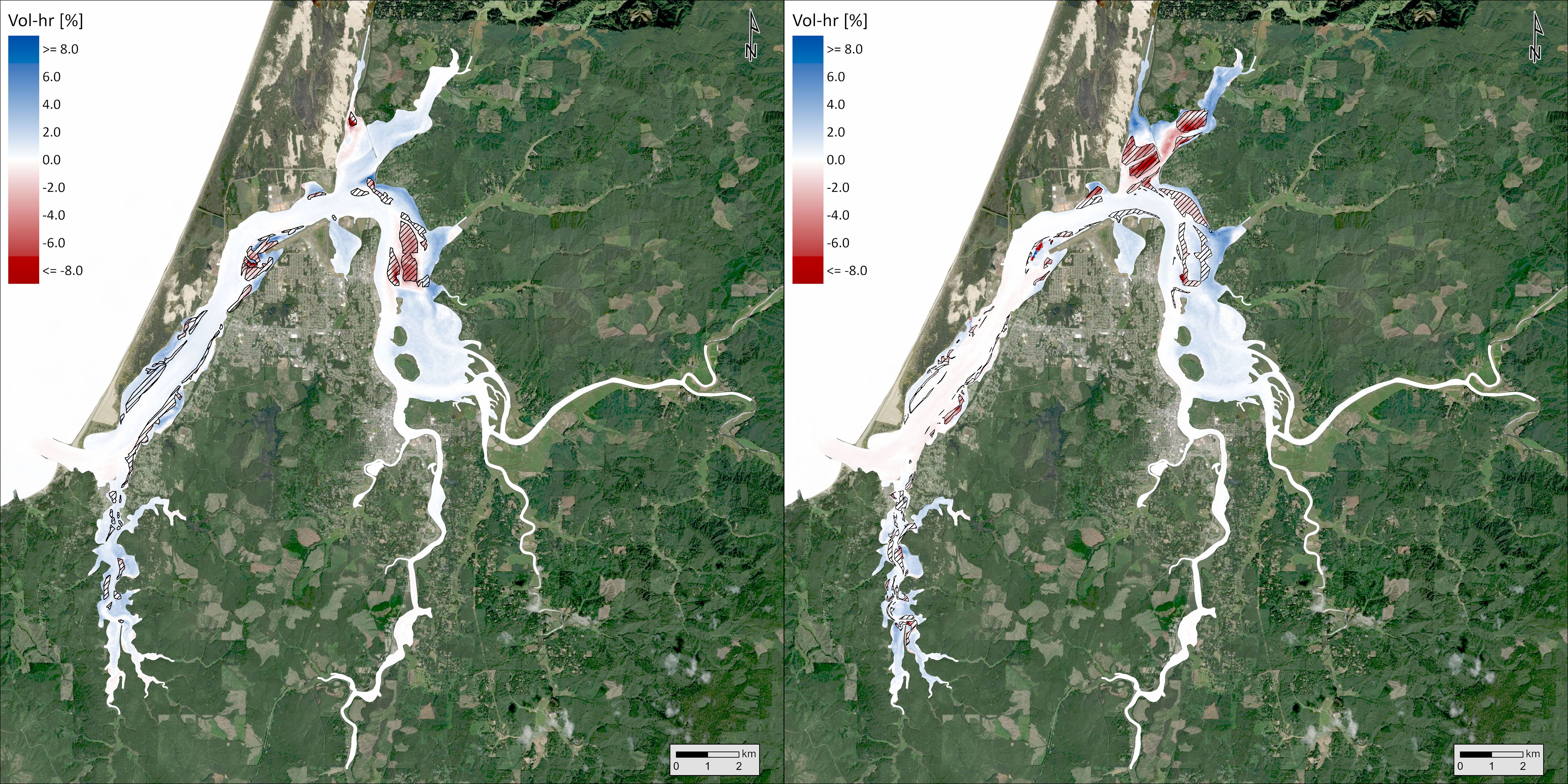
Figure 10. Change in the fraction volume-hour that dissolved oxygen is < 6.5 mg/L between current extent and no eelgrass scenarios (left) and maximum extent and current scenarios (right). Hatched areas indicate where eelgrass was added to the model between scenarios.

Figure 11

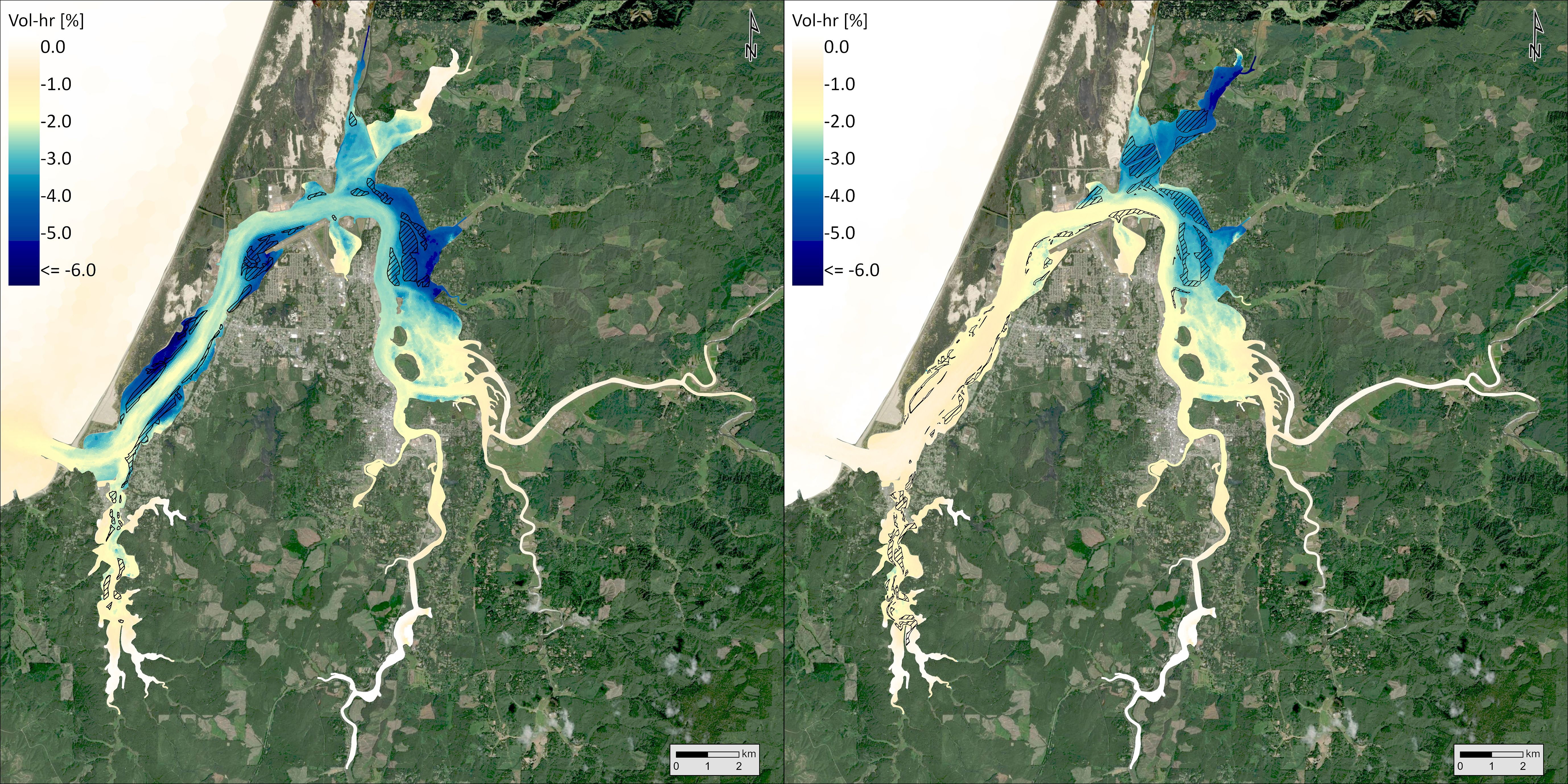
Figure 11. Change in the fraction volume-hour that pH is < 7.8 between current extent and no eelgrass scenarios (left) and maximum extent and current scenarios (right). Hatched areas indicate where eelgrass was added to the model between scenarios.

Figure 12

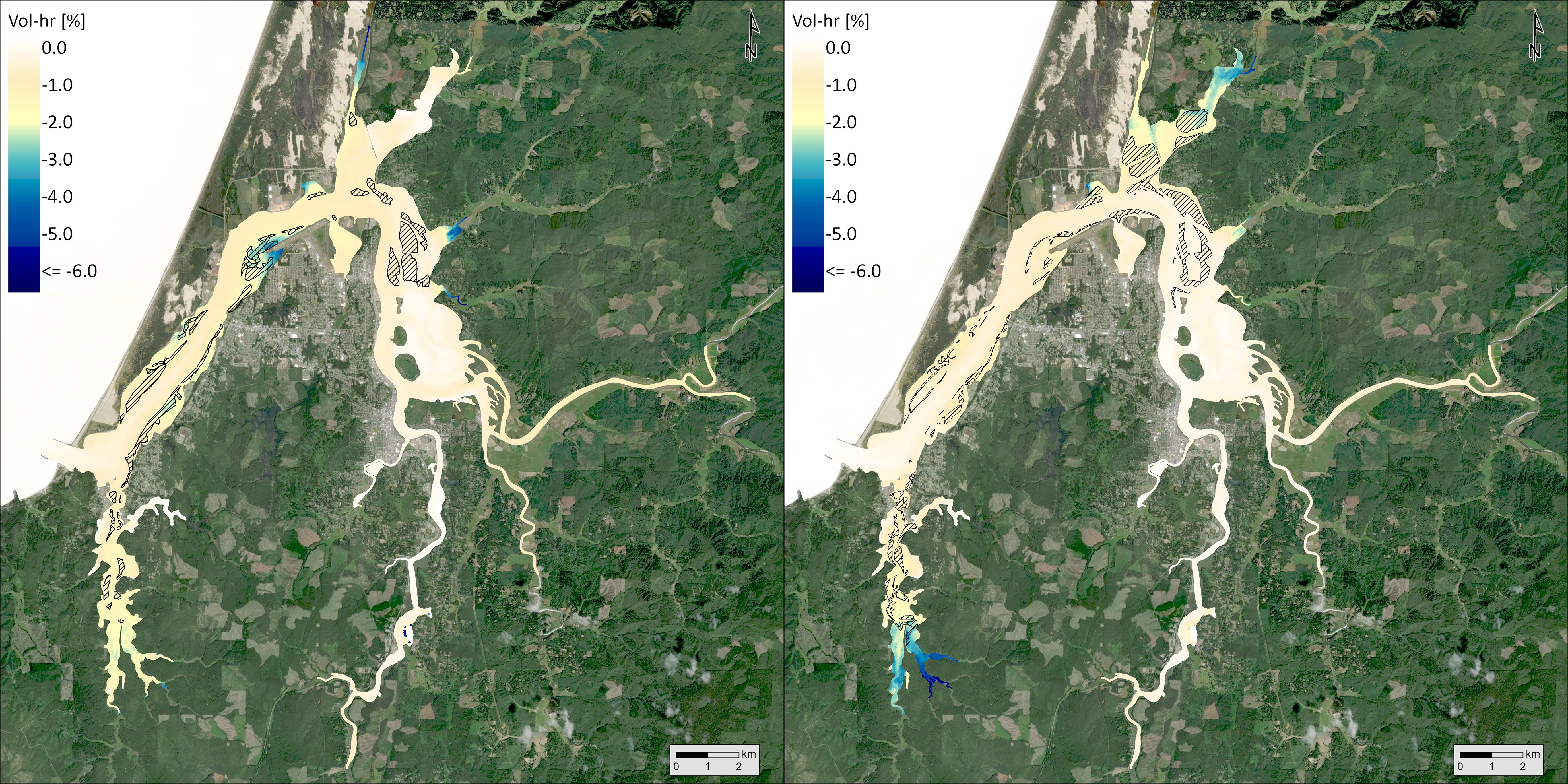
Figure 12. Change in the fraction volume-hour that the calcium carbonate saturation state for aragonite (Ω) is < 1 between current extent and no eelgrass scenarios (left) and maximum extent and current scenarios (right). Hatched areas indicate where eelgrass was added to the model between scenarios.

4 Discussion

Using an existing hydrodynamic model, previously collected water quality and eelgrass observations, and a biogeochemical model framework, we developed a biophysical model of Coos Bay, Oregon that simulates water quality and eelgrass (Zostera marina) dynamics and was capable of reproducing observed biogeochemical dynamics with moderate skill. We then used the model to run scenarios of eelgrass extent and evaluate the resulting ocean acidification and hypoxia (OAH) conditions. The ability of seagrasses, including eelgrass, to mitigate the low DO, low pH, and corrosive conditions associated with OAH continues to be debated (Van Dam et al., 2021a; Van Dam et al., 2021b; Garner et al., 2022) and is critical for understanding the value of eelgrass conservation and restoration. Our new model represents a useful tool - one which accounts for and controls the relevant physical and biogeochemical processes - to evaluate conditions that confer resilience or enhance vulnerability to OAH in an important Pacific Northwest (PNW) coastal estuary.

We found that including eelgrass in the biophysical model of Coos Bay produced results that more closely resembled the temporal variability in water quality observations - the models with eelgrass simulated dissolved oxygen (DO) and pH conditions that were more dynamic, often having both higher highs and lower lows due to the combined influence of photosynthesis and respiration. These dynamics align with the highly variable conditions found across PNW estuaries (Brown and Nelson, 2015; Sutherland and O’Neill, 2016) and the findings of other studies of eelgrass mitigation (Magel et al., 2023; Pacella et al., 2018, 2024). In part due to this dynamism, evidence for hypoxia mitigation by eelgrass in Coos Bay at an estuary-wide scale was spatially and temporally limited in the model simulations. There were some areas of the estuary where DO conditions improved with the addition of eelgrass, but overall there was a small net increase in harmful DO concentrations (based on volume-hours below 6.5 mg/L - a physiological threshold for salmon). These modeling results align with a monitoring study in Coos Bay, which found that eelgrass biomass across 15 years and three sites in the South Slough arm was positively related to maximum DO, but negatively related to mean and minimum DO (Magel et al., 2023). In contrast, ocean acidification conditions, pH and aragonite saturation state, were improved with the addition of eelgrass (based on volume-hours below 7.8 pH and Ω = 1 thresholds for Olympia oysters). Although the minimum pH was not always changed, median and maximum pH were elevated in models with eelgrass by 0.04 to 0.13 and 0.27 to 0.99 pH units, respectively (Table 2). Because the pH scale is logarithmic, this represents up to a ten-fold decrease in acidity. Even small changes in pH could have significant biological benefits to species, particularly during critical early life history periods (Waldbusser et al., 2015). As expected, OAH mitigation was more common during summer when eelgrass productivity is high and plants are net autotrophic. These findings also align with results of the Magel et al. (2023) monitoring study, which found that there was a positive relationship between summer eelgrass biomass and maximum, mean, and to a lesser extent minimum pH in Coos Bay.

At a within-estuary scale, there were differences between sites indicating that certain locations within the estuary may be more well-suited for eelgrass mitigation of OAH. Results at Charleston, located near the mouth of the estuary, showed less change in pH and DO compared to Valino and BLM (Figures 8, 9). This finding aligns with the work of Magel et al. (2023), which found no influence of interannual differences in eelgrass biomass on the diel dynamics of DO or pH at the Charleston site (called “Barview” in that paper), compared to Valino and another site in South Slough where eelgrass biomass was positively correlated with DO and pH. Magel et al. (2023) hypothesized that larger tidal exchange and shorter residence times in the Charleston/Barview region of Coos Bay (Sutherland and O’Neill, 2016; Eidam et al., 2020) limited the influence of eelgrass on water column conditions (Magel et al., 2023). Our spatial analysis of volume-hr changes also indicated that improvements in pH and DO conditions are more likely to occur in areas of eelgrass that are shallower, more tidally restricted (Figures 10-12). Another modeling approach also identified water depth and residence time as important factors determining OA mitigation by eelgrass (Koweek et al., 2018). Eelgrass beds located in shallow areas with less tidal flushing, similar to Valino and BLM, may be better suited to OA mitigation.

The expansion of eelgrass coverage in the maximum observed extent scenario resulted in additional increases in pH at Valino and Charleston, but not at BLM. This likely has to do with the configuration of eelgrass beds in the two scenarios - eelgrass area increased more between the current and maximum extent scenarios close to the Valino and Charleston sites compared to BLM (Figure 2). The average biomass of eelgrass at beds in those locations was consistent between scenarios and is unlikely to have contributed to the observed differences in pH dynamics (Supplementary Figure 14). The additional changes in DO dynamics moving from the current extent to the maximum observed extent scenario were very minor at all three sites.

The presence of eelgrass in any given area of Coos Bay did not guarantee reduced exposure to harmful DO concentrations, but improvements were likely in areas where eelgrass was added to the model – in most cases the benefits for DO did not extend beyond the area of the beds (Figure 10). For pH and saturation state, however, conditions were generally improved across the estuary (Figures 11, 12). The largest improvements in pH were within the areas of eelgrass beds but also extended beyond beds (Figure 11). The spatial and temporal dependencies of eelgrass mitigation of OAH in Coos Bay align with the findings of other studies that have found seagrass can exacerbate OAH in some circumstances (Cyronak et al., 2018; Koweek et al., 2018; Pacella et al., 2018). The water column chemistry in seagrass habitats is influenced by many biogeochemical and physical processes that act - and interact - over short (hours, days) and long timescales (seasons, years) (Duarte et al., 2013). Our model results represent the combined influence of biogeochemical and physical processes in Coos Bay for Y2014. Pacella et al. (2018) found that the potential for eelgrass mitigation of OA increases with higher atmospheric CO₂ levels (end of century predictions) indicating that future carbonate system conditions may be increasingly favorable for OA mitigation by eelgrass. Given that future carbon conditions could influence eelgrass growth (Palacios and Zimmerman, 2007; Zimmerman et al., 2015) and mitigation potential (Pacella et al., 2018), future climate modeling would be improved by including carbon limitation kinetics on eelgrass growth in the model. At present, the eelgrass submodel of FVCOM-ICM includes the kinetics of temperature and nutrient controls on eelgrass growth but not dissolved inorganic carbon. As a result, the Khangaonkar et al. (2021a) application of FVCOM-ICM to project future climate impacts on eelgrass in Puget Sound, WA shows only reductions in eelgrass biomass due to elevated temperatures and no potential impact from greater carbon availability.

4.1 Model building and performance

Completion of the model of Coos Bay represents a significant technical advancement for understanding the dynamics of the estuary and the responses of complex biophysical parameters to alternative scenarios. Further, we believe this is the first application of the eelgrass submodel using FVCOM-ICM to a whole-estuary and the second to use the eelgrass submodel – Khangaonkar et al. (2021a) was the first, which implemented eelgrass in a single, small embayment within the Salish Sea Model. Now that the model has been built, it can be used to explore additional research questions about changes in climate (e.g., marine heatwaves, sea level rise, drought), ocean processes (e.g., upwelling intensity), or land use (e.g., nutrient loading, freshwater flow timing and intensity) in Coos Bay. Similar applications of FVCOM-ICM have been explored using the Salish Sea Model and found important interactions between estuarine biogeochemistry and those drivers (Bianucci et al., 2018; Khangaonkar et al., 2018, 2019; Khangaonkar et al., 2021a, b). However, we encountered several challenges in creating and validating the biophysical model of Coos Bay which may have impacted the performance of the model and could influence its applicability to future research and management questions.

First, there were data availability issues that challenged model development and validation. Observations for the freshwater rivers and streams entering Coos Bay were lacking and we had to apply broad generalizations to the freshwater model inputs for temperature, nutrients, and carbon. This could explain poorer model performance in certain locations or during certain time periods. Estuarine water quality and eelgrass observations were also somewhat limited - particularly in the upper reaches of the northern, Coos River arm (Figure 1). For eelgrass, belowground biomass data was particularly lacking (only available at two sites) and more is needed to further validate performance of the eelgrass submodel. Sampling of belowground biomass is more destructive to the eelgrass bed and is more time consuming to collect and process compared to aboveground biomass, which may partially explain the comparative lack of belowground data. Additional data collection targeting these gaps might help to improve performance of the model or further validate existing model behavior. It is worth noting, however, that behavior of the FVCOM-ICM eelgrass submodel was parameterized based on Z. marina in another PNW estuary and the belowground biomass values produced by the Coos Bay model are within the range of observations for this species in PNW estuaries (Khangaonkar et al., 2021a; Magel, 2020).

Second, there were challenges in simulating the water quality model (FVCOM-ICM) in Coos Bay which may also explain some of the differences in model performance over space and time. During the calibration process of the model, we encountered significant challenges, particularly with the sediment oxygen demand which periodically caused the model to crash, resulting in negative dissolved oxygen (DO) values in certain eelgrass bed areas. To mitigate this problem, we excluded the problematic eelgrass regions from the model, resulting in a slightly smaller total eelgrass area. The wetting and drying scheme of FVCOM is not well adapted in the FVCOM-ICM and is likely the source of the invalid result. Improvements to the wetting and drying scheme in the water quality model may improve the predictions in shallow subtidal and intertidal zones and eliminate this issue. In application of the same model framework to the Salish Sea, Washington and British Columbia, Khangaonkar et al. (2021a) masked results in the shallow subtidal and intertidal areas due to a lack of confidence in model performance in those areas and a lack of data with which to validate model performance. The discrepancies in these regions highlight the need for further improvement in the water quality model framework (FVCOM-ICM) and model calibration in shallow subtidal and intertidal zones. Improving and testing the model for this specific issue was beyond the scope of our project.

Lastly, we reduced complexity of the existing hydrodynamic model for Coos Bay (Conroy et al., 2020) in order to significantly reduce computational time required to run the offline water quality model, including reducing the number of model nodes and layers and smoothing bathymetry. While these alterations did not significantly reduce performance of salinity in the lower and mid estuary, using the more complex model may have improved performance of other water quality parameters. Simulated salinity in the transition zone where tidal forces compete with river discharge can be improved by increasing horizontal and vertical model resolutions to better resolve the sharp stratification gradient and tidal asymmetry (Ralston and Geyer, 2019) and may be important for model applications focused on this area of the estuary. However, tradeoffs between performance and computational time/power are important considerations.

4.2 Ecosystem impacts

It is difficult to translate the predicted chemical changes in Coos Bay into species responses and an improvement in OAH conditions does not necessarily produce a biological benefit (Cossa et al., 2024; Greiner et al., 2018; Garner et al., 2022). Our understanding of the short and long term effects of OAH exposure - as individual stressors and in combination - on species and their overall tolerance and sensitivity is still evolving and is further complicated by the potential for local adaptation within certain species (Cossa et al., 2024; Hofmann et al., 2014; Gobler and Baumann, 2016; Vargas et al., 2017). Additional synergistic stressors, such as temperature and shifting community structure, add additional complexity to species’ responses and the ability of seagrass to mitigate the negative effects of OAH (Egea et al., 2024; Kroeker et al., 2016). If the spatial or temporal improvements in OAH conditions coincide with locations or windows of a species’ heightened sensitivity, there are likely to be benefits to that species. Furthermore, increases or longer durations of pH or DO maxima during the daytime due to seagrass photosynthesis may help species to tolerate the lower lows that occur at night. Daily increases in pH maxima may be more important than increases in average pH for some species (Price et al., 2012). While an in-depth discussion is outside the scope of this paper, it is worth noting that seagrasses also enhance long term storage or sequestration of carbon belowground, which contributes to their purported role in combating climate change (Fourqurean et al., 2012; Stankovic et al., 2021). However, the impact of future conditions on seagrass carbon sequestration is debated and with future ocean acidification and increased temperature this service could either be enhanced (Yamuza-Magdaleno et al., 2025) or reduced (Dahl et al., 2023). The benefits and ecosystem services of seagrass extend well beyond that of OAH mitigation or carbon sequestration (Costanza et al., 1997), so it is important to remember that even in circumstances where seagrass exacerbates harmful OAH conditions or where species do not respond, there is still a net positive influence of seagrass on the ecosystem.

4.3 Management implications for Coos Bay

There are multiple factors to consider when managing eelgrass in Coos Bay (and other estuaries), including the current and future suitability of environmental conditions for eelgrass, likelihood of persistence or restoration success, human and social needs, and the ecosystem services provided by eelgrass compared to other potential nearshore habitats. From an OAH mitigation perspective only, our modeling study suggests three general areas of focus for eelgrass conservation and restoration in Coos Bay: 1) the shallow margins of the main channel, such as Fossil Point, Pigeon Point, and the flat across from BLM; 2) the large, intertidal flats of the northern Coos River arm, such as those adjacent to Haynes Inlet and East Bay; and 3) the upper reaches of South Slough, including Winchester and Elliot Creek (Figure 1). While Magel et al. (2023) found eelgrass biomass to be a determining factor in DO and pH impacts at individual sites, biomass was less important at an estuary-wide scale and also was not a primary determinant of mitigation in our model. Areas of highest biomass, such as the marine dominated Charleston/Barview area, had lower evidence for mitigation of OAH compared to other lower biomass areas. Physical factors, such as residence time and depth, and other biogeochemical factors may be more important for determining mitigation.

Climate impacts, including future temperature and sea level rise conditions, should be considered in planning for climate resilient eelgrass beds in Coos Bay. Water temperature was a primary driver of the recent eelgrass declines in Coos Bay (Marin Jarrin et al., 2022; Magel et al., 2023) and the shallow areas well suited for OAH mitigation mentioned above may be less resilient to climate change because they tend to be warmer. Sea-level rise could serve to buffer temperature impacts on shallow beds, however, if rising ocean water levels increase inundation (reducing desiccation stress) and limit warming due to greater exchange of cold, ocean water. Maintaining water clarity is critical for resilient eelgrass beds because it helps to combat the impact of warm temperatures (Moore et al., 2012), disease (Vergeer et al., 1995), and the loss of deeper beds with sea level rise (Shaughnessy et al., 2012). Evaluating these interacting climate factors using the biophysical model of Coos Bay would further refine eelgrass management recommendations.

5 Conclusion

Biophysical ecosystem models are powerful tools for the study of eelgrass mitigation of OAH because they allow us to account for both large and fine scale biogeochemical processes, control all aspects of the system, and examine the results at both large and fine spatial and temporal scales. These modeling studies complement in situ field and lab experiments and observations. Building the biophysical model of Coos Bay allowed us to evaluate the impact of eelgrass extent scenarios on Coos Bay water quality, including pH, DO, and calcium carbonate saturation state, and results can inform eelgrass conservation and restoration. The model can now be used to explore additional research questions about changes in climate (e.g., marine heatwaves, sea level rise, drought), ocean processes (e.g., upwelling intensity), or land use (e.g., nutrient loading, freshwater flow timing and intensity) in Coos Bay. Future projects should consider whether improvements to the model structure or input data are needed to adequately address these questions.

Data availability statement

The original contributions presented in the study are included in the article/Supplementary Material, further inquiries can be directed to the corresponding author/s.

Author contributions

CM: Conceptualization, Data curation, Formal analysis, Funding acquisition, Project administration, Visualization, Writing – original draft, Writing – review & editing. AN: Data curation, Formal analysis, Methodology, Validation, Visualization, Writing – original draft, Writing – review & editing. DS: Conceptualization, Data curation, Software, Writing – review & editing. AH: Conceptualization, Data curation, Methodology, Writing – review & editing. JN: Conceptualization, Data curation, Writing – review & editing. TK: Conceptualization, Funding acquisition, Project administration, Software, Supervision, Writing – review & editing.

Funding

The author(s) declare that financial support was received for the research and/or publication of this article. This work was funded by the Oregon Ocean Science Trust, in consultation with the Oregon Coordinating Council on Ocean Acidification and Hypoxia, under an award to the University of Washington.

Acknowledgments

The authors gratefully acknowledge the many groups who have contributed to water quality and eelgrass data collection in the Coos Bay estuary over the last several decades, including South Slough National Estuarine Research Reserve, local tribes (Confederated Tribes of Coos, Lower Umpqua and Siuslaw Indians and Coquille Indian Tribe), researchers (J. Hayduk and M. Hessing-Lewis), and state and federal agencies (Oregon Department of Fish and Wildlife, Oregon Department of Environmental Quality, U.S. Environmental Protection Agency). These datasets have made our work possible. We also thank Kevin Bogue, who provided GIS support for maps and figures.

Conflict of interest

The authors declare that the research was conducted in the absence of any commercial or financial relationships that could be construed as a potential conflict of interest.

Generative AI statement

The author(s) declare that no Generative AI was used in the creation of this manuscript.

Publisher’s note

All claims expressed in this article are solely those of the authors and do not necessarily represent those of their affiliated organizations, or those of the publisher, the editors and the reviewers. Any product that may be evaluated in this article, or claim that may be made by its manufacturer, is not guaranteed or endorsed by the publisher.

Supplementary material

The Supplementary Material for this article can be found online at: https://www.frontiersin.org/articles/10.3389/fmars.2025.1585621/full#supplementary-material

References

Abe H., Ito M. A., Ahn H., and Nakaoka M. (2022). Eelgrass beds can mitigate local acidification and reduce oyster malformation risk in a subarctic lagoon, Japan: A three-dimensional ecosystem model study. Ocean Model. 173, 101992. doi: 10.1016/j.ocemod.2022.101992

Crossref Full Text | Google Scholar

Banas N. S., Conway-Cranos L., Sutherland D. A., MacCready P., Kiffney P., and Plummer M. (2015). Patterns of river influence and connectivity among subbasins of puget sound, with application to bacterial and nutrient loading. Estuaries Coasts 38, 735–753. doi: 10.1007/s12237-014-9853-y

Crossref Full Text | Google Scholar

Bancroft M. P. (2015). An Experimental Investigation of the Effects of Temperature and Dissolved Oxygen on the Growth of Juvenile English Sole and Juvenile Dungeness Crab. Oregon State University, Corvallis, Oregon, USA.

Google Scholar

Barbier E. B., Hacker S. D., Kennedy C., Koch E. W., Stier A. C., and Silliman B. R. (2011). The value of estuarine and coastal ecosystem services. Ecol. Monogr. 81, 169–193. doi: 10.1890/10-1510.1

Crossref Full Text | Google Scholar

Barton A., Hales B., Waldbusser G. G., Langdon C., and Feely R. A. (2012). The Pacific oyster, Crassostrea gigas, shows negative correlation to naturally elevated carbon dioxide levels: Implications for near-term ocean acidification effects. Limnology Oceanography 57, 698–710. doi: 10.4319/lo.2012.57.3.0698

Crossref Full Text | Google Scholar

Bednaršek N., Feely R. A., Beck M. W., Alin S. R., Siedlecki S. A., Calosi P., et al. (2020). Exoskeleton dissolution with mechanoreceptor damage in larval Dungeness crab related to severity of present-day ocean acidification vertical gradients. Sci. Total Environ. 716, 136610. doi: 10.1016/j.scitotenv.2020.136610

PubMed Abstract | PubMed Abstract | Crossref Full Text | Google Scholar

Bergstrom E., Silva J., Martins C., and Horta P. (2019). Seagrass can mitigate negative ocean acidification effects on calcifying algae. Sci. Rep. 9. doi: 10.1038/s41598-018-35670-3

PubMed Abstract | PubMed Abstract | Crossref Full Text | Google Scholar

Bianucci L., Long W., Khangaonkar T., Pelletier G., Ahmed A., Mohamedali T., et al. (2018). Sensitivity of the regional ocean acidification and carbonate system in Puget Sound to ocean and freshwater inputs. Edited by Jody W. Deming and Lisa A. Miller. Elementa: Sci. Anthropocene 6, 22. doi: 10.1525/elementa.151

Crossref Full Text | Google Scholar

Boyer T. P., García H. E., Locarnini R. A., Zweng M. M., Mishonov A. V., Reagan J. R., et al. (2018). World Ocean Atlas 2018. NOAA National Centers for Environmental Information. Dataset. Available online at: https://www.ncei.noaa.gov/archive/accession/NCEI-WOA18.

Google Scholar

Brett J. R. and Blackburn J. M. (1981). Oxygen requirements for growth of young coho (Oncorhynchus kisutch) and sockeye (O. nerka) Salmon at 15°C. Can. J. Fisheries Aquat. Sci. 38, 399–404. doi: 10.1139/f81-056

Crossref Full Text | Google Scholar

Brown C. A. and Nelson W. G. (2015). A method to identify estuarine water quality exceedances associated with ocean conditions. Environ. Monitoring Assess. 187, 133. doi: 10.1007/s10661-015-4347-3

PubMed Abstract | PubMed Abstract | Crossref Full Text | Google Scholar

Brown C. A., Nelson W. G., Boese B. L., DeWitt T. H., Eldridge P. M., Kaldy J. E., et al. (2007). An approach to developing nutrient criteria for Pacific Northwest estuaries: a case study of Yaquina Estuary, Oregon. USEPA Office Res. Development Natl. Health Environ. Effects Laboratory Western Ecol. Division 169. doi: 10.5962/bhl.title.149777

Crossref Full Text | Google Scholar

Brown C. A. and Ozretich R. J. (2009). Coupling between the coastal ocean and Yaquina Bay, Oregon: Importance of oceanic inputs relative to other nitrogen sources. Estuaries Coasts 32, 219–237. doi: 10.1007/s12237-008-9128-6

Crossref Full Text | Google Scholar

Cerco C. F. and Cole T. (1993). Three-dimensional eutrophication model of chesapeake bay. J. Environ. Eng. 119, 1006–1025. doi: 10.1061/(ASCE)0733-9372(1993)119:6(1006

Crossref Full Text | Google Scholar

Cerco C. F. and Cole T. M. (1995). User’s guide to the CE-QUAL-ICM three-dimensional eutrophication model: release version 1.0. Report. Environ. Lab. (U.S.), 320. Available online at: https://erdc-library.erdc.dren.mil/items/81b728f7-7b2e-4ef8-e053-411ac80adeb3

Google Scholar

Cerco C. F. and Noel M. R. (2013). Twenty-one-year simulation of chesapeake bay water quality using the CE-QUAL-ICM eutrophication model. JAWRA J. Am. Water Resour. Assoc. 49, 1119–1133. doi: 10.1111/jawr.12107

Crossref Full Text | Google Scholar

Chen C., Liu H., and Beardsley R. C. (2003). An unstructured grid, finite-volume, three-dimensional, primitive equations ocean model: application to coastal ocean and estuaries. J. Atmospheric Oceanic Technol. 20, 159–186. doi: 10.1175/1520-0426(2003)020<0159:AUGFVT>2.0.CO;2

Crossref Full Text | Google Scholar

Conroy T., Sutherland D. A., and Ralston D. K. (2020). Estuarine exchange flow variability in a seasonal, segmented estuary. J. Phys. Oceanography 50, 595–613. doi: 10.1175/JPO-D-19-0108.1

Crossref Full Text | Google Scholar

Cossa D., Infantes E., and Dupont S. (2024). Hidden cost of pH variability in seagrass beds on marine calcifiers under ocean acidification. Sci. Total Environ. 915, 170169. doi: 10.1016/j.scitotenv.2024.170169

PubMed Abstract | PubMed Abstract | Crossref Full Text | Google Scholar

Costanza R., d’Arge R., de Groot R., Farber S., Grasso M., Hannon B., et al. (1997). The value of the world’s ecosystem services and natural capital. Nature 387, 253–260. doi: 10.1038/387253a0

Crossref Full Text | Google Scholar

Cyronak T., Andersson A. J., D’Angelo S., Bresnahan P., Davidson C., Griffin A., et al. (2018). Short-term spatial and temporal carbonate chemistry variability in two contrasting seagrass meadows: implications for pH buffering capacities. Estuaries Coasts 41, 1282–1296. doi: 10.1007/s12237-017-0356-5

Crossref Full Text | Google Scholar

Dahl M., McMahon K., Lavery P. S., Hamilton S. H., Lovelock C. E., and Serrano O. (2023). Ranking the risk of CO₂ emissions from seagrass soil carbon stocks under global change threats. Global Environ. Change 78, 102632. doi: 10.1016/j.gloenvcha.2022.102632

Crossref Full Text | Google Scholar

Davis K. A., Banas N. S., Giddings S. N., Siedlecki S. A., MacCready P., Lessard E. J., et al. (2014). Estuary-enhanced upwelling of marine nutrients fuels coastal productivity in the U.S. Pacific Northwest. J. Geophysical Research: Oceans 119, 8778–8799. doi: 10.1002/2014JC010248

Crossref Full Text | Google Scholar

Doney S. C., Fabry V. J., Feely R. A., and Kleypas J. A. (2009). Ocean acidification: the other CO₂ problem. Annu. Rev. Marine Sci. 1, 169–192. doi: 10.1146/annurev.marine.010908.163834

PubMed Abstract | PubMed Abstract | Crossref Full Text | Google Scholar

Duarte C. M. (1990). Seagrass nutrient content. Marine Ecol. Prog. Ser. 67, 201–207. doi: 10.3354/meps067201

Crossref Full Text | Google Scholar

Duarte C. M. and Cebrian J. (1996). The fate of marine autotrophic production. Limnology Oceanography 41, 1758–1766. doi: 10.4319/lo.1996.41.8.1758

Crossref Full Text | Google Scholar

Duarte C. M., Hendriks I. E., Moore T. S., Olsen Y. S., Steckbauer A., Ramajo L., et al. (2013). Is ocean acidification an open-ocean syndrome? Understanding anthropogenic impacts on seawater pH. Estuaries Coasts 36, 221–236. doi: 10.1007/s12237-013-9594-3

Crossref Full Text | Google Scholar

Egea L. G., Jiménez-Ramos R., English M. K., Tomas F., and Mueller R. S. (2024). Marine heatwaves and disease alter community metabolism and DOC fluxes on a widespread habitat-forming seagrass species (Zostera marina). Sci. Total Environ. 957, 177820. doi: 10.1016/j.scitotenv.2024.177820

PubMed Abstract | PubMed Abstract | Crossref Full Text | Google Scholar

Eidam E., Souza T., Keogh M., Sutherland D., Ralston D. K., Schmitt J., et al. (2024). Spatial and temporal variability of century-scale sediment accumulation in an active-margin estuary. Estuaries Coasts 47, 2267–2282. doi: 10.1007/s12237-024-01407-x

Crossref Full Text | Google Scholar

Eidam E. F., Sutherland D. A., Ralston D. K., Dye B., Conroy T., Schmitt J., et al. (2020). Impacts of 150 years of shoreline and bathymetric change in the coos estuary, oregon, USA. Estuaries Coasts 45, 1170–1188. doi: 10.1007/s12237-020-00732-1

Crossref Full Text | Google Scholar

Feely R. A., Alin S. R., Carter B., Bednaršek N., Hales B., Chan F., et al. (2016). Chemical and biological impacts of ocean acidification along the west coast of North America. Estuarine Coastal Shelf Sci. 183, 260–270. doi: 10.1016/j.ecss.2016.08.043

Crossref Full Text | Google Scholar

Fourqurean J. W., Duarte C. M., Kennedy H., Marbà N., Holmer M., Mateo M. A., et al. (2012). Seagrass ecosystems as a globally significant carbon stock. Nat. Geosci. 5, 505–509. doi: 10.1038/ngeo1477

Crossref Full Text | Google Scholar

Fourqurean J. W., Moore T. O., Fry B., and Hollibaugh J. T. (1997). Spatial and temporal variation in C:N:P ratios, δ15N, and δ13C of eelgrass Zostera marina as indicators of ecosystem processes, Tomales Bay, California, USA. Marine Ecol. Prog. Ser. 157, 147–157. doi: 10.3354/meps157147

Crossref Full Text | Google Scholar

Garner N., Ross P. M., Falkenberg L. J., Seymour J. R., Siboni N., and Scanes E. (2022). Can seagrass modify the effects of ocean acidification on oysters? Marine Pollution Bull. 177, 113438. doi: 10.1016/j.marpolbul.2022.113438

PubMed Abstract | PubMed Abstract | Crossref Full Text | Google Scholar

Gobler C. J. and Baumann H. (2016). Hypoxia and acidification in ocean ecosystems: coupled dynamics and effects on marine life. Biol. Lett. 12, 20150976. doi: 10.1098/rsbl.2015.0976

PubMed Abstract | PubMed Abstract | Crossref Full Text | Google Scholar

Grantham B. A., Chan F., Nielsen K. J., Fox D. S., Barth J. A., Huyer A., et al. (2004). Upwelling-driven nearshore hypoxia signals ecosystem and oceanographic changes in the northeast Pacific. Nature 429, 749–754. doi: 10.1038/nature02605

PubMed Abstract | PubMed Abstract | Crossref Full Text | Google Scholar

Gregory D. N. (2004). Ocean Data Inventory (ODI): A Database of Ocean Current, Temperature and Salinity Time Series for the Northwest Atlantic (Fisheries and Oceans Canada, Dartmouth, Canada: DFO Canadian Science Advisory Secretariat Research Document 2004/097[4]).

Google Scholar

Greiner C. M., Klinger T., Ruesink J. L., Barber J. S., and Horwith M. (2018). Habitat effects of macrophytes and shell on carbonate chemistry and juvenile clam recruitment, survival, and growth. J. Exp. Marine Biol. Ecol. 509, 8–15. doi: 10.1016/j.jembe.2018.08.006

Crossref Full Text | Google Scholar

Gruber N., Hauri C., Lachkar Z., Loher D., Frölicher T. L., and Plattner G.-K. (2012). Rapid progression of ocean acidification in the California Current System. Science 337, 220–223. doi: 10.1126/science.1216773

PubMed Abstract | PubMed Abstract | Crossref Full Text | Google Scholar

Hayduk J. L., Hacker S. D., Henderson J. S., and Tomas F. (2019). Evidence for regional-scale controls on eelgrass (Zostera marina) and mesograzer community structure in upwelling-influenced estuaries. Limnology Oceanography 64, 1120–1134. doi: 10.1002/lno.11102

Crossref Full Text | Google Scholar

Hendriks I. E., Olsen Y. S., Ramajo L., Basso L., Steckbauer A., Moore T. S., et al. (2014). Photosynthetic activity buffers ocean acidification in seagrass meadows. Biogeosciences 11, 333–346. doi: 10.5194/bg-11-333-2014

Crossref Full Text | Google Scholar

Hessing-Lewis M. L., Hacker S. D., Menge B. A., and Rumrill S. S. (2011). Context-dependent eelgrass–macroalgae interactions along an estuarine gradient in the Pacific Northwest, USA. Estuaries Coasts 34, 1169–1181. doi: 10.1007/s12237-011-9412-8

Crossref Full Text | Google Scholar

Hettinger A., Sanford E., Hill T. M., Russell A. D., Sato K. N., Hoey J., et al. (2012). Persistent carry-over effects of planktonic exposure to ocean acidification in the Olympia oyster. Ecology 93, 2758–2768. doi: 10.1890/12-0567.1

PubMed Abstract | PubMed Abstract | Crossref Full Text | Google Scholar

Hofmann G. E., Evans T. G., Kelly M. W., Padilla-Gamiño J. L., Blanchette C. A., Washburn L., et al. (2014). Exploring local adaptation and the ocean acidification seascape &ndash; studies in the California Current Large Marine Ecosystem. Biogeosciences 11, 1053–1064. doi: 10.5194/bg-11-1053-2014

Crossref Full Text | Google Scholar

Hood R. R., Shenk G. W., Dixon R. L., Smith S. M. C., Ball W. P., Bash J. O., et al. (2021). The Chesapeake Bay program modeling system: Overview and recommendations for future development. Ecol. Modelling 456, 109635. doi: 10.1016/j.ecolmodel.2021.109635

PubMed Abstract | PubMed Abstract | Crossref Full Text | Google Scholar

Irby I. D., Friedrichs M. A. M., Da F., and Hinson K. E. (2018). The competing impacts of climate change and nutrient reductions on dissolved oxygen in Chesapeake Bay. Biogeosciences 15, 2649–2668. doi: 10.5194/bg-15-2649-2018

Crossref Full Text | Google Scholar

Kennish M. J. (2021). Drivers of change in estuarine and coastal marine environments: an overview. Open J. Ecol. 11, 224. doi: 10.4236/oje.2021.113017

Crossref Full Text | Google Scholar

Keogh M. E., Sutherland D. A., Eidam E. F., Souza T. D., Schmitt J., Helms A., et al. (2025). Estuarine sediment dynamics and the importance of storms in moving (and removing) mud. Estuaries Coasts 48, 1–17. doi: 10.1007/s12237-025-01524-1

Crossref Full Text | Google Scholar

Khangaonkar T., Nugraha A., Premathilake L., Keister J., and Borde A. (2021a). Projections of algae, eelgrass, and zooplankton ecological interactions in the inner Salish Sea – for future climate, and altered oceanic states. Ecol. Modelling 441, 109420. doi: 10.1016/j.ecolmodel.2020.109420

Crossref Full Text | Google Scholar

Khangaonkar T., Nugraha A., Xu W., and Balaguru K. (2019). Salish sea response to global climate change, sea level rise, and future nutrient loads. J. Geophysical Research: Oceans 124, 3876–3904. doi: 10.1029/2018JC014670

Crossref Full Text | Google Scholar

Khangaonkar T., Nugraha A., Xu W., Long W., Bianucci L., Ahmed A., et al. (2018). Analysis of hypoxia and sensitivity to nutrient pollution in Salish Sea. J. Geophysical Research: Oceans 123, 4735–4761. doi: 10.1029/2017JC013650

Crossref Full Text | Google Scholar

Khangaonkar T., Nugraha A., Yun S. K., Premathilake L., Keister J. E., and Bos J. (2021b). Propagation of the 2014–2016 northeast pacific marine heatwave through the salish sea. Front. Marine Sci. 8. doi: 10.3389/fmars.2021.787604

Crossref Full Text | Google Scholar

Khangaonkar T., Sackmann B., Long W., Mohamedali T., and Roberts M. (2012). Simulation of annual biogeochemical cycles of nutrient balance, phytoplankton bloom(s), and DO in Puget Sound using an unstructured grid model. Ocean Dynamics 62, 1353–1379. doi: 10.1007/s10236-012-0562-4

Crossref Full Text | Google Scholar

Khangaonkar T., Yang Z., Kim T., and Roberts M. (2011). Tidally averaged circulation in Puget Sound sub-basins: Comparison of historical data, analytical model, and numerical model. Estuarine Coastal Shelf Sci. 93, 305–319. doi: 10.1016/j.ecss.2011.04.016

Crossref Full Text | Google Scholar

Kim T. and Khangaonkar T. (2012). An offline unstructured biogeochemical model (UBM) for complex estuarine and coastal environments. Environ. Model. Softw. 31, 47–63. doi: 10.1016/j.envsoft.2011.11.010

Crossref Full Text | Google Scholar

Klinger T., Chornesky E. A., Whiteman E. A., Chan F., Largier J. L., and Wakefield W. W. (2017). Using integrated, ecosystem-level management to address intensifying ocean acidification and hypoxia in the California Current large marine ecosystem. Elementa: Sci. Anthropocene 5, 16. doi: 10.1525/elementa.198

Crossref Full Text | Google Scholar

Koch M., Bowes G., Ross C., and Zhang X.-H. (2013). Climate change and ocean acidification effects on seagrasses and marine macroalgae. Global Change Biol. 19, 103–132. doi: 10.1111/j.1365-2486.2012.02791.x

PubMed Abstract | PubMed Abstract | Crossref Full Text | Google Scholar

Koweek D. A., Zimmerman R. C., Hewett K. M., Gaylord B., Giddings S. N., Nickols K. J., et al. (2018). Expected limits on the ocean acidification buffering potential of a temperate seagrass meadow. Ecol. Appl. 28, 1694–1714. doi: 10.1002/eap.1771

PubMed Abstract | PubMed Abstract | Crossref Full Text | Google Scholar

Kroeker K. J., Sanford E., Rose J. M., Blanchette C. A., Chan F., Chavez F. P., et al. (2016). Interacting environmental mosaics drive geographic variation in mussel performance and predation vulnerability. Ecol. Lett. 19, 771–779. doi: 10.1111/ele.12613

PubMed Abstract | PubMed Abstract | Crossref Full Text | Google Scholar

Lincoln S., Vannoni M., Benson L., Engelhard G. H., Tracey D., Shaw C., et al. (2021). Assessing intertidal seagrass beds relative to water quality in Vanuatu, South Pacific. Mar. Pollut. Bull. 163, 111936. doi: 10.1016/j.marpolbul.2020.111936

PubMed Abstract | PubMed Abstract | Crossref Full Text | Google Scholar

Liu P.-J., Ang S.-J., Mayfield A. B., and Lin H.-J. (2020). Influence of the seagrass Thalassia hemprichii on coral reef mesocosms exposed to ocean acidification and experimentally elevated temperatures. Sci. Total Environ. 700, 134464. doi: 10.1016/j.scitotenv.2019.134464

PubMed Abstract | PubMed Abstract | Crossref Full Text | Google Scholar

Long M. H., Sutherland K., Wankel S. D., Burdige D. J., and Zimmerman R. C. (2020). Ebullition of oxygen from seagrasses under supersaturated conditions. Limnology Oceanography 65, 314–324. doi: 10.1002/lno.11299

PubMed Abstract | PubMed Abstract | Crossref Full Text | Google Scholar

MacCready P., McCabe R. M., Siedlecki S. A., Lorenz M., Giddings S. N., Bos J., et al. (2021). Estuarine circulation, mixing, and residence times in the salish sea. J. Geophysical Research: Oceans 126, e2020JC016738. doi: 10.1029/2020JC016738

Crossref Full Text | Google Scholar

Magel C. L. (2020). Ecosystem Functions of Pacific Northwest Estuaries: The Role of Ocean and Watershed Drivers in Eelgrass and Coho Salmon Dynamics (Corvallis, Oregon, USA: Oregon State University).

Google Scholar

Magel C. L., Hacker S. D., Chan F., and Helms A. R. (2023). Eelgrass and macroalgae loss in an oregon estuary: consequences for ocean acidification and hypoxia. Ocean-Land-Atmosphere Res. 2, 23. doi: 10.34133/olar.0023

Crossref Full Text | Google Scholar

Marin Jarrin M. J., Sutherland D. A., and Helms A. R. (2022). Water temperature variability in the Coos Estuary and its potential link to eelgrass loss. Front. Marine Sci. 9. doi: 10.3389/fmars.2022.930440

Crossref Full Text | Google Scholar

Marshall K. N., Kaplan I. C., Hodgson E. E., Hermann A., Busch D. S., McElhany P., et al. (2018). Risks of ocean acidification in the California Current food web and fisheries: ecosystem model projections. Global Change Biol. 23, 1525–1539. doi: 10.1111/gcb.13594

PubMed Abstract | PubMed Abstract | Crossref Full Text | Google Scholar

Moore K. A. (2013). NERRS SWMP Vegetation Monitoring Protocol: long-term monitoring of estuarine vegetation communities. Vegetation Monitoring Workgroup (Gloucester Point, VA: Chesapeake Bay National Estuarine Research Reserve System).

Google Scholar

Moore K. A., Shields E. C., Parrish D. B., and Orth R. J. (2012). Eelgrass survival in two contrasting systems: role of turbidity and summer water temperatures. Marine Ecol. Prog. Ser. 448, 247–258. doi: 10.3354/meps09578

Crossref Full Text | Google Scholar

Moriasi D. N., Gitau M. W., Pai N., and Daggupati P. (2015). Hydrologic and water quality models: performance measures and evaluation criteria. Trans. Am. Soc. Agric. Biol. Engineers 58, 1763–1785. doi: 10.13031/trans.58.10715

Crossref Full Text | Google Scholar

Orr J. C., Epitalon J.-M., Dickson A. G., and Gattuso J.-P. (2018). Routine uncertainty propagation for the marine carbon dioxide system. Marine Chem. 207, 84–107. doi: 10.1016/j.marchem.2018.10.006

Crossref Full Text | Google Scholar

Pacella S. R., Brown C. A., Labiosa R. G., Hales B., Mochon Collura T. C., Evans W., et al. (2024). Feedbacks between estuarine metabolism and anthropogenic CO2 accelerate local rates of ocean acidification and hasten threshold exceedances. J. Geophysical Research: Oceans 129, e2023JC020313. doi: 10.1029/2023JC020313

PubMed Abstract | PubMed Abstract | Crossref Full Text | Google Scholar

Pacella S. R., Brown C. A., Waldbusser G. G., Labiosa R. G., and Hales B. (2018). Seagrass habitat metabolism increases short-term extremes and long-term offset of CO₂ under future ocean acidification. Proc. Natl. Acad. Sci. 115, 3870–3875. doi: 10.1073/pnas.1703445115

PubMed Abstract | PubMed Abstract | Crossref Full Text | Google Scholar

Palacios S. and Zimmerman R. (2007). Response of eelgrass Zostera marina to CO2 enrichment: possible impacts of climate change and potential for remediation of coastal habitats. Marine Ecol. Prog. Ser. 344, 1–13. doi: 10.3354/meps07084

Crossref Full Text | Google Scholar

Price N. N., Martz T. R., Brainard R. E., and Smith J. E. (2012). Diel variability in seawater pH relates to calcification and benthic community structure on coral reefs. PloS One 7, e43843. doi: 10.1371/journal.pone.0043843

PubMed Abstract | PubMed Abstract | Crossref Full Text | Google Scholar

Ralston D. K. and Geyer W. R. (2019). Response to channel deepening of the salinity intrusion, estuarine circulation, and stratification in an urbanized estuary, J. Geophys. Res.-Ocean. 124, 4784–4802. doi: 10.1029/2019JC015006

Crossref Full Text | Google Scholar

Ricart A. M., Ward M., Hill T. M., Sanford E., Kroeker K. J., Takeshita Y., et al. (2021). Coast-wide evidence of low pH amelioration by seagrass ecosystems. Global Change Biol. 27, 2580–2591. doi: 10.1111/gcb.15594

PubMed Abstract | PubMed Abstract | Crossref Full Text | Google Scholar

Rumrill S. (2006). The Ecology of the South Slough Estuary: Site Profile of the South Slough National Estuarine Research Reserve. NOAA, Salem, OR.

Google Scholar

Sampaio E., Santos C., Rosa I. C., Ferreira V., Pörtner H.-O., Pörtner H.-O., et al. (2021). Impacts of hypoxic events surpass those of future ocean warming and acidification. Nat. Ecol. Evol., 311–321. doi: 10.1038/s41559-020-01370-3

PubMed Abstract | PubMed Abstract | Crossref Full Text | Google Scholar

Shaughnessy F. J., Gilkerson W., Black J. M., Ward D. H., and Petrie M. (2012). Predicted eelgrass response to sea level rise and its availability to foraging Black Brant in Pacific coast estuaries. Ecol. Appl. 22, 1743–1761. doi: 10.1890/11-1083.1

PubMed Abstract | PubMed Abstract | Crossref Full Text | Google Scholar

Sherman K. and DeBruyckere L. A. (2018). Eelgrass habitats on the U.S. West coast: state of the knowledge of eelgrass ecosystem services and eelgrass extent. Pacific Marine Estuarine Fish Habitat Partnership Nat. Conservancy. 67.

Google Scholar

Siedlecki S. A., Banas N. S., Davis K. A., Giddings S., Hickey B. M., MacCready P., et al. (2015). Seasonal and interannual oxygen variability on the Washington and Oregon continental shelves. J. Geophysical Research: Oceans 120, 608–633. doi: 10.1002/2014JC010254

Crossref Full Text | Google Scholar

Stankovic M., Ambo-Rappe R., Carly F., Dangan-Galon F., Fortes M. D., Hossain M. S., et al. (2021). Quantification of blue carbon in seagrass ecosystems of Southeast Asia and their potential for climate change mitigation. Sci. Total Environ. 783, 146858. doi: 10.1016/j.scitotenv.2021.146858

PubMed Abstract | PubMed Abstract | Crossref Full Text | Google Scholar

Sutherland D. A. and O’Neill M. A. (2016). Hydrographic and dissolved oxygen variability in a seasonal Pacific Northwest estuary. Estuarine Coastal Shelf Sci. 172, 47–59. doi: 10.1016/j.ecss.2016.01.042

Crossref Full Text | Google Scholar

Thom R. M., Borde A. B., Rumrill S., Woodruff D. L., Williams G. D., Southard J. A., et al. (2003). Factors influencing spatial and annual variability in eelgrass (Zostera marina L.) meadows in Willapa Bay, Washington, and Coos Bay, Oregon, estuaries. Estuaries 26, 1117–1129. doi: 10.1007/BF02803368

Crossref Full Text | Google Scholar

Unsworth R. K. F. and Cullen-Unsworth L. C. (2014). “Biodiversity, ecosystem services, and the conservation of seagrass meadows,” in Coastal Conservation. Eds. Maslo B. and Lockwood J. L. (Cambridge University Press, Cambridge), 95–130. doi: 10.1017/CBO9781139137089.005

Crossref Full Text | Google Scholar

Valiela I. (1995). Marine ecological processes (New York, NY: Springer-Verlag).

Google Scholar

Van Dam B., Lopes C., Zeller M. A., Ribas-Ribas M., Wang H., and Thomas H. (2021a). Overstated potential for seagrass meadows to mitigate coastal ocean acidification. Front. Marine Sci. 8. doi: 10.3389/fmars.2021.729992

Crossref Full Text | Google Scholar

Van Dam B. R., Zeller M. A., Lopes C., Smyth A. R., Böttcher M. E., Osburn C. L., et al. (2021b). Calcification-driven CO₂ emissions exceed “Blue Carbon“ sequestration in a carbonate seagrass meadow. Sci. Adv. 7, eabj1372. doi: 10.1126/sciadv.abj1372

PubMed Abstract | PubMed Abstract | Crossref Full Text | Google Scholar

Vargas C. A., Lagos N. A., Lardies M. A., Duarte C., Manríquez P. H., Aguilera V. M., et al. (2017). Species-specific responses to ocean acidification should account for local adaptation and adaptive plasticity. Nat. Ecol. Evol. 1, 1–7. doi: 10.1038/s41559-017-0084

PubMed Abstract | PubMed Abstract | Crossref Full Text | Google Scholar

Vergeer L. H. T., Aarts T. L., and de Groot J. D. (1995). The ‘wasting disease’ and the effect of abiotic factors (light intensity, temperature, salinity) and infection with Labyrinthula zosterae on the phenolic content of Zostera marina shoots. Aquat. Bot. 52, 35–44. doi: 10.1016/0304-3770(95)00480-N

Crossref Full Text | Google Scholar

Waldbusser G. G., Hales B., Langdon C. J., Haley B. A., Schrader P., Brunner E. L., et al. (2015). Saturation-state sensitivity of marine bivalve larvae to ocean acidification. Nat. Climate Change 5, 273–280. doi: 10.1038/nclimate2479

Crossref Full Text | Google Scholar

Waldbusser G. G. and Salisbury J. E. (2014). Ocean acidification in the coastal zone from an organism’s perspective: Multiple system parameters, frequency domains, and habitats. Annu. Rev. Marine Sci. 6, 221–247. doi: 10.1146/annurev-marine-121211-172238

PubMed Abstract | PubMed Abstract | Crossref Full Text | Google Scholar

Walter R. K., O’Leary J. K., Vitousek S., Taherkhani M., Geraghty C., and Kitajima A. (2020). Large-scale erosion driven by intertidal eelgrass loss in an estuarine environment. Estuarine Coastal Shelf Sci. 243, 106910. doi: 10.1016/j.ecss.2020.106910

Crossref Full Text | Google Scholar

Waycott M., Duarte C. M., Carruthers T. J. B., Orth R. J., Dennison W. C., Olyarnik S., et al. (2009). Accelerating loss of seagrasses across the globe threatens coastal ecosystems. Proc. Natl. Acad. Sci. 106, 12377–12381. doi: 10.1073/pnas.0905620106

PubMed Abstract | PubMed Abstract | Crossref Full Text | Google Scholar

Willmott C. J. (1982). Some comments on the evaluation of model performance. Bull. Am. Meteorological Soc. 63, 1309–1313. doi: 10.1175/1520-0477(1982)063<1309:SCOTEO>2.0.CO;2

Crossref Full Text | Google Scholar

Yamuza-Magdaleno A., Jiménez-Ramos R., Cavijoli-Bosch J., Brun F. G., and Egea L. G. (2025). Ocean acidification and global warming may favor blue carbon service in a Cymodocea nodosa community by modifying carbon metabolism and dissolved organic carbon fluxes. Marine Pollution Bull. 212, 117501. doi: 10.1016/j.marpolbul.2024.117501

PubMed Abstract | PubMed Abstract | Crossref Full Text | Google Scholar

Zimmerman R. C., Hill V. J., and Gallegos C. L. (2015). Predicting effects of ocean warming, acidification, and water quality on Chesapeake region eelgrass: Predicting eelgrass response to climate change. Limnology Oceanography 60, 1781–1804. doi: 10.1002/lno.10139

Crossref Full Text | Google Scholar