Abstract
In recent years, the accuracy of ocean forecasts has significantly improved thanks to spatial altimetry. However, despite their importance, forecasting accurate currents is still a challenge. Therefore, satellite missions are proposed to provide measurements of surface velocity on a global coverage. The Ocean DYnamics and Surface Exchange with the Atmosphere (ODYSEA) mission of the National Aeronautics and Space Administration (NASA) and Centre National d’Etudes Spatiales (CNES) is currently competing for selection in the Earth System Explorers program. As part of the preliminary studies for ODYSEA, we have carried out Observing System Simulation Experiments (OSSEs) to assess the impact of assimilating these prospective observations in terms of Root Mean Square differences of the model state variables to a reference run. We focus on disentangling the impact of the ODYSEA observations from the impact of the observations provided by altimetry, on large scale, and checking the complementarity of these networks to avoid redundant information. We show that zonal velocity out of the Equator, sea surface height and surface salinity are mainly constrained by altimetry. Conversely, the meridional velocity is mainly constrained by velocity observations. Moreover, these latter observations help better prescribing both components of velocity at the Equator as well as the sea surface temperature in the Eastern Pacific. They also tend to significantly improve surface salinity in some regions where freshwater input occurs. Altimetry and surface velocity observations are complementary, and when they are assimilated together, all the model state variables are improved in all regions compared to assimilating altimetry only.
1 Introduction
Over the past 50 years, satellite altimetry has seen its capacity multiplied. Sea level anomaly (SLA) observations have become more and more accurate, and satellite constellations are now providing a massive amount of data. Long experience in assimilating these observations along with other observations such as sea surface temperature (SST) or temperature and salinity profiles has led to efficient ocean analysis and forecasting systems (e.g. Lellouche et al., 2018). Through data assimilation schemes, SLA observations effectively improve the initial conditions of the sea surface height (SSH) analyses and forecasts. They also contribute to correcting temperature and salinity through their relationship with the baroclinic component of SLA and density (Weaver et al., 2005).
In the Mercator Ocean International (MOI) analysis and forecasting system, no velocity observations are assimilated operationally. Therefore, the corrections brought to the initial conditions of the zonal and meridional velocity analyses and forecasts are calculated through their relationship with the other variables. In particular, SLA observations help to correct the geostrophic currents (Isern-Fontanet et al., 2017), which are the dominant currents out of the equator. They also contribute to improve to some extent the wind-driven components of the currents through the pressure gradient induced by the wind. In an inter-comparison between different ocean monitoring systems and velocity observations derived from drifters, Aijaz et al. (2023) found that in the MOI system, the stronger zonal mean currents are generally better represented than the smaller meridional mean currents. Moreover, better accuracy is obtained in regions where currents are strong and well-defined (e.g. Tropics) compared to areas dominated by eddies and high kinetic energy. However, even if a good correlation is found between the model currents and the observations (drogued drifters), the model currents are generally underestimated.
Forecasting accurate surface ocean velocities is essential for many applications, such as rescue operations, pollutant tracking or ship routing. Although using SLA observations to correct the currents has shown a significant efficiency, it still has some limitations. First, the northward component of the geostrophic current is generally poorly observed due to the orientation north/south of the altimetry track (Isern-Fontanet et al., 2017). This means that the SLA observations help to correct mainly the zonal velocity rather than the meridional velocity. This is a possible explanation for the results seen by Aijaz et al. (2023). Secondly, SLA corrections can affect only some components of the current (the geostrophic and partly the wind-driven components). However, they cannot inform on most of the ageostrophic components (Rio et al., 2014, for the Ekman component).
Recently, different satellite missions have been proposed to measure Total Surface Current Velocities (TSCV), i.e. the sum of all the different current contributions (geostrophic, wind-driven, wave-induced), on a global coverage. Among the candidates, the Ocean DYnamics and Surface Exchange with the Atmosphere (ODYSEA) mission of the National Aeronautics and Space Administration (NASA) proposes the use of a Doppler scatterometer to measure on a wide swath surface winds and currents at high-resolution (Torres et al., 2023). Considering the benefit of SLA observations despite their limitations, it is fair to wonder what such surface velocity observations could bring further to analysis and forecasting systems. In this perspective, Observing System Simulation Experiments (OSSEs; Hoffman and Atlas, 2016) have been run to try and disentangle the benefit of each of these types of data.
This study follows previous OSSEs of the same kind that have been run recently for the Sea Surface KInematics Multiscale (SKIM) project funded by the European Space Agency (ESA) to assess the general impact of assimilating that kind of observations. Both the Met Office (Waters et al., 2024a) and MOI (Mirouze et al., 2024) found that assimilating TSCV data was beneficial, especially at the Equator. A comparison of their results is also reported in Waters et al. (2024b). As a complement to this previous study, we are trying in this brief research report to disentangle the impact of the ODYSEA observations from the impact of the observations provided by conventional altimetry, on large scale. The idea is to check the complementarity of these networks to limit redundant information. Note that assimilating observations simulated for ODYSEA rather than SKIM confirms the previous general results despite the differences in the satellites.
The design and the experiments are presented in section 2, while the results are analyzed in section 3. A discussion is then proposed in section 4.
2 Method
In this section, we briefly present the design of the OSSEs that have been run.
2.1 Design of the experiments
The design of these OSSEs follows the design of the previous OSSEs run for the SKIM project, with some updates. Although a short description is provided below, the interested reader should refer to Mirouze et al. (2024) for more details.
The study has been carried out using the new MOI analysis and forecasting system in development, associating the ocean model NEMO 4.2 (Madec et al., 2022) and the sea ice model SI3 (Vancoppenolle et al., 2023). The analysis and forecast are made on the 1/4° ORCA grid, with an extension in the Antarctic. The horizontal resolution ranges from 27 km at the Equator to 6 km at high latitudes. The vertical grid is composed of 75 levels, the first level representing 1 m. Hourly ERA5 fields (Hersbach et al., 2020) are used as atmosphere forcing. The data assimilation system is based on the singular evolutive extended Kalman Filter formulation (SEEK; Pham et al., 1998; Brasseur and Verron, 2006). The background error covariances contain univariate and multivariate structures and are calculated from a collection of anomalies provided by a long run of about 10 years assimilating observations (Benkiran et al., 2021).
Classically, observations of SST, temperature and salinity in-situ vertical profiles (ARGO, Drifters, Moorings, XBT), SLA and Sea Ice Concentration (SIC) are assimilated to define correctional increments that are applied through an incremental analysis update (IAU; Bloom et al., 1996) procedure. Here, pseudo-observations are simulated from the so-called Nature Run (NR), with a random error added as explained in Mirouze et al. (2024) and Mao et al. (2020) for SIC observations. SLA observations are simulated as data provided by 5 nadir altimeters (Altika, Cryosat2, Jason3, Sentinel 3A and 3B). They are used to calculate a misfit with respect to the model SSH. This model SSH is referred to the geoïd, and corresponds to what the altimetry calls the Absolute Dynamic Topography (ADT)1, i.e. the addition of SLA to the Mean Dynamic Topography (MDT). The misfit calculation consists in subtracting the MDT to the model SSH and compare this model SLA to the SLA observations. To avoid any artificial impact, the MDT to be subtracted must be consistent with the NR. Therefore, the model SSH is directly used to simulate the altimetry observations. However, in the rest of the paper, we will keep the term “SLA observations” to prevent any confusion. The NR is a free simulation without any data assimilation, run with version 3.1 of NEMO (Madec, 2008) and the LIM sea ice model (Vancoppenolle et al., 2009). The resolution is 1/12° horizontally with 50 vertical levels. The atmospheric forcing is provided by the European Center for Medium-range Weather Forecasts (ECMWF) at a three-hour frequency.
Observations of TSCV and their associated instrument error are also simulated from the NR using a specific ODYSEA simulator reproducing the future satellite tracks2,3,4. Since the NR does not account for tides nor Stokes drift, these contributions are not included in the observations. The Eastward and Northward velocity components are reconstructed from the radial velocity using a bi-variate weighted least square approach. This procedure introduces a mapping random error which standard deviation is about 2 cm/s. The instrument random error is estimated depending on the wind speed and direction, and the position on the swath across-track. Indeed, a certain roughness of the sea surface is required to obtain a good measurement of the current velocity. The instrument error is the dominant error and its standard deviation varies from a few cm/s away from the nadir and the swath edges with a high wind speed to more than 1 m/s under the nadir or in regions without any wind. The prescribed observation error includes the mapping and instrument errors. It also includes a representativity random error to account for scales existing in the ocean model at a resolution of 1/12° but unresolved at 1/4°. Observations with a high prescribed error standard deviation (> 1.5 m/s) are discarded. Considering the large ODYSEA swath of about 1500 km and the resolution of 5 km x 5 km of the observations, only 1 over 8 observations across- and along-track are assimilated5.
2.2 Experiments
Three experiments have been conducted for comparison. All experiments have exactly the same configuration and ancillary files. They use the same restart files on 31 December 2008 and are run until 29 December 2009. The observations of SST, temperature and salinity profiles, and SIC are assimilated in all the experiments, using a 7-day assimilation window. The three experiments differ in the type of observations they assimilate in addition: SLA only, TSCV only, or both SLA and TSCV. Specifically, the experiments are: (i) ASMsla, which assimilates only SLA observations; (ii) ASMtscv, which assimilates only TSCV observations; and (iii) ASMboth, which assimilates both SLA and TSCV observations.
ASMsla is the so-called control of the OSSEs. It represents the closest configuration to the current operational system. Any improvement seen in the other experiments compared to it means that assimilating ODYSEA TSCV data is beneficial. ASMtscv is a specific experiment that is not realistic, since it does not assimilate SLA, which are existing and useful observations. It is designed to help disentangle the impact of TSCV data from the impact of SLA data in the analysis, when compared to ASMsla. Finally, ASMboth represents the potential future analysis, should TSCV data become available.
3 Results
The difference between the daily average ocean state of each experiment and the daily average state of the NR interpolated on the OSSE grid has been computed. Statistics of mean and root mean square (RMS) of these differences have then been calculated from 1st February 2009 to 29 December 2009, January being discarded since it is considered as a spin-up allowing for the ocean state to stabilize. In this section, we compare these statistics (summarized in Table 1) to assess the impact of assimilating ODYSEA TSCV data on the model state variables. This comparison is limited to the surface, although it is clear that both SLA and TSCV observations have an impact on the water column through spatial and multivariate covariances.
Table 1
| Global | Equator | Gulf Stream | Malvinas | Agulhas | Kuroshio | ACC | |
|---|---|---|---|---|---|---|---|
| SSU |
0.9 cm/s
(11%) |
4.5 cm/s
(27%) |
0.5 cm/s
(4%) |
0.2 cm/s
(3%) |
0.3 cm/s
(3%) |
0.3 cm/s
(3%) |
0.3 cm/s
(5%) |
| SSV |
1.1 cm/s
(14%) |
3 cm/s
(22%) |
1 cm/s
(9%) |
0.6 cm/s
(8%) |
0.1 cm/s
(10%) |
0.8 cm/s
(9%) |
0.8 cm/s
(11%) |
| SST |
< 0.01 °C
(1%) |
0.03 °C
(9%) |
0.01 °C
(1%) |
< 0.01 °C
(2%) |
< 0.01 °C
(2%) |
< 0.01 °C
(2%) |
< 0.01 °C
(< 1%) |
| SSS |
< 0.01psu
(< 1%) |
< 0.01psu
(< 1%) |
< 0.01psu
(< 1%) |
< 0.01psu
(< 1%) |
< 0.01psu
(2%) |
< 0.01psu
(1%) |
0.02psu
(4%) |
| SSH |
0.1 cm
(3%) |
0.1 cm
(9%) |
0.3 cm
(7%) |
0.2 cm
(5%) |
0.2 cm
(6%) |
0.2 cm
(5%) |
0.2 cm
(5%) |
RMS improvement for the surface variables in ASMboth compared to ASMsla, calculated from 01/02/2009 to 29/12/2009.
Bold green indicates a significant improvement greater than 5%; green (red) indicates a small improvement (degradation); and light green (light red) indicate a non-significant improvement (degradation).
3.1 Velocity
As shown on Figures 1a, b, the zonal velocity is mainly constrained by SLA observations outside the Equator, whereas the meridional velocity is mainly constrained by TSCV observations. As already mentioned, one of the limitations of the satellite altimetry is that the geostrophic currents are mainly observed in the eastward direction. SLA observations can therefore help to correct the zonal velocity but have smaller impact on the meridional velocity. Therefore, the latter fully takes advantage of the assimilation of the TSCV data. However, it is surprising to see the importance of zonal velocity RMS degradation that reaches 8% to 10% in the Western Boundary Currents (WBCs) and the Antarctic Circumpolar Current (ACC), and even up to 16% in the Malvinas region. A possible explanation comes from the TSCV observation instrument error, which has a higher magnitude in the eastward direction than in the northward direction6. Another reason could come from conflicts between the corrections brought by the TSCV data and the corrections brought by temperature and salinity observations not being constrained by SLA observations and therefore misplacing eddies. It is worth mentioning that no specific tuning has been performed for these OSSEs. Therefore, some improvement might be expected with proper adjustment.
Figure 1

Difference (ASMtscv – NR) RMS – (ASMsla – NR) RMS (a, b), and (ASMboth – NR) RMS – (ASMsla – NR) RMS (c, d) for surface zonal (a, c) and surface meridional (b, d) velocity calculated from 01/02/2009 to 29/12/2009. Blue (red) areas indicate that ASMtscv or ASMboth (ASMsla) is closer to NR.
When both types of observation are assimilated (Figures 1c, d), the velocity RMS is improved by 3% to 5% for the zonal component and 8% to 11% for the meridional component in the WBCs and the ACC. For the meridional velocity, about 70% of the RMS improvement comes from the TSCV observations. Even in the Malvinas region where the RMS was slightly degraded (2%) a notable improvement of 8% is achieved when both types of observations are assimilated. This suggests that the assimilated TSCV data add an extra benefit to the SLA observations, and that the two datasets are complementary. It is possible that the TSCV observations bring information on the ageostrophic part of the currents, the wind driven component in particular, that SLA observations cannot.
The Equator is the region the most impacted by the TSCV data. Assimilating them allows the RMS to be improved by 25% and 19% for zonal and meridional velocity, respectively. When SLA observations are associated, an additional improvement of 2% to 3% is obtained. The Equatorial Currents being wind-driven currents, SLA observations struggle to fully constrain them. It is therefore consistent that the greatest impact of the TSCV observations is seen in this region.
It is worth mentioning that the improvement seen in the analysis is maintained in 7-day forecasts.
3.2 Other variables
SLA and TSCV observations are not the main constraint of surface temperature. This is consistent with the fact that SST maps are assimilated and thus more legitimate in correcting the sea surface temperature. However, we can see a significant improvement in the SST RMS in the eastern equatorial Pacific caused by TSCV observations (Figures 2a–c). This location corresponds to the NINO boxes that are used to forecast the El Niño Southern Oscillation (ENSO) events. For example, the NINO3.4 box between 120W and 170W is used to monitor the SST and calculate the Oceanic Niño Index (ONI), while the Trans-Niño Index (TNI) informs on the SST gradient in the region (Trenberth and Stepaniak, 2001). This suggests that a better representation of the equatorial currents could be a key to improving the accuracy of ENSO predictions.
Figure 2
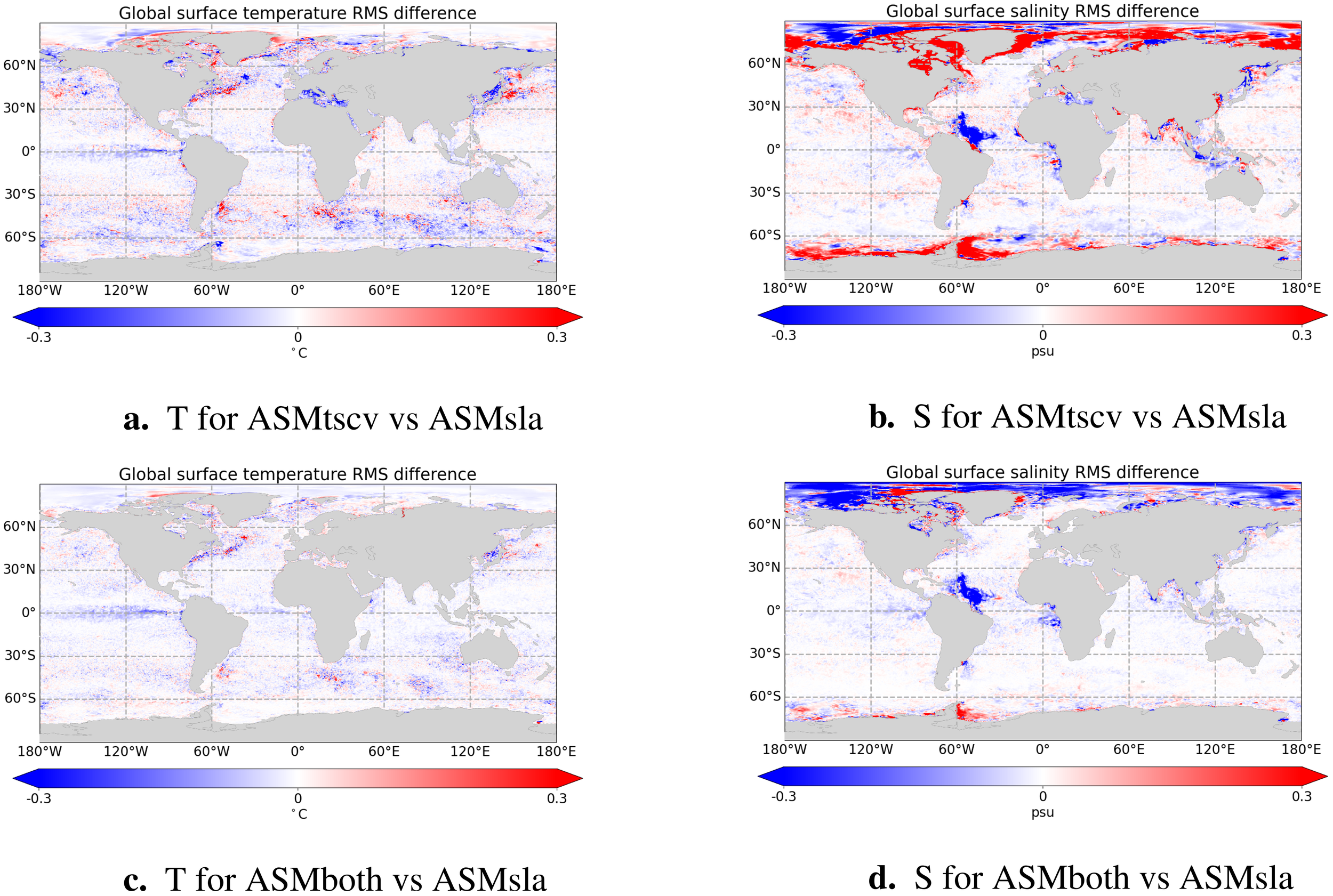
Difference (ASMtscv – NR) RMS – (ASMsla – NR) RMS (a, b), and (ASMboth – NR) RMS –(ASMsla – NR) RMS (c, d) for surface temperature (a, c) and surface salinity (b, d) calculated from 01/02/2009 to 29/12/2009. Blue (red) areas indicate that ASMtscv or ASMboth (ASMsla) is closer to NR.
In these OSSEs, surface salinity is poorly observed since the salinity profiles assimilated start a few meters below the surface. The corrections for surface salinity depend on these profiles but also on SST and SSH via the multivariate covariances. Differences between the experiments are globally very small and caution must be taken when using percentages to express them. As shown in Figures 2b–d, the surface salinity RMS is slightly improved in the Tropics when both SLA and TSCV observations are assimilated. We also note a large improvement in river outflow regions such as the Amazon and the Congo plumes, most of this improvement coming from the TSCV observations rather than the SLA observations. This suggests that a better representation of the equatorial currents leads to a better representation of the freshwater circulation. However, such an important improvement is a little unexpected and therefore, further analysis is required to make sure that it is genuine.
When SLA observations are not assimilated, the surface salinity RMS is generally degraded in the Arctic Ocean. It turns into a large improvement however, when both SLA and TSCV data are assimilated. This is especially true in summer (not shown), when the ice is melted and has brought an important volume of freshwater in the ocean. Meanwhile, the salinity RMS is also largely improved along the East Iceland Current and the Baffin Current. This suggests again that a better representation of these currents helps better represent the freshwater circulation. Note that these currents have a strong meridional component and are hence benefiting the most from TSCV observations. Again, such an important improvement is a little unexpected and therefore, further analysis is required to make sure that it is genuine. Near the Antarctic on the contrary, a degradation can be seen near the coasts. This is probably due to the fact that we start the assessment at the end of the austral summer. Therefore, ice is present most of the assessment time or in the process of melting or icing. Moreover, the 1/4° grid we are running the OSSEs with has a grid that defines better the Antarctic coasts than the NR. A part of the degradation might come from the interpolation of the NR fields with a different bathymetry in that region.
Apart from the regions mentioned above, surface temperature and salinity are not really impacted by TSCV observations. The slight degradations in the surface salinity RMS that can be spotted when SLA observations are not assimilated are generally restrained to tens of meters below the surface.
SLA observations are clearly the main constraint for SSH (Figure 3). However, when TSCV observations are assimilated in addition to SLA data, the SSH RMS is globally improved by 3%. The best improvement is seen at the Equator (9%) and reaches 5% to 7% in the WBCs and the ACC. This is an interesting feature that suggests that velocity observations can also help to correct SSH through the multivariate covariances, showing again how SLA and TSCV observations are complementary.
Figure 3
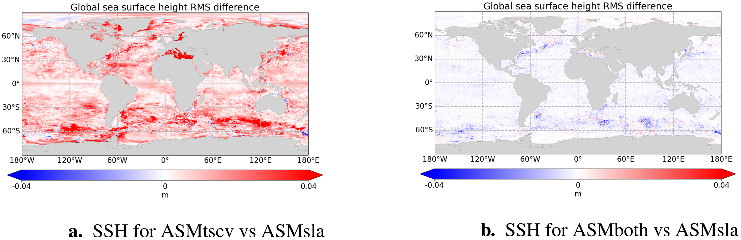
Difference (ASMtscv – NR) RMS – (ASMsla – NR) RMS (a), and (ASMboth – NR) RMS – (ASMsla – NR) RMS (b) for SSH calculated from 01/02/2009 to 29/12/2009. Blue (red) areas indicate that ASMtscv or ASMboth (ASMsla) is closer to NR.
3.3 Summary
Table 1 summarizes the improvement (green) or degradation (red) of RMS for the different variables in different regions when TSCV data are assimilated in addition to SLA observations. The surface velocity and the SSH RMS are improved in all regions. For surface temperature and salinity, the differences are generally non-significant, except for the SST at the Equator, which is due to the important improvement in the Eastern Equatorial Pacific. We note a small degradation for surface salinity in the ACC due to the degradations near the coasts of Antarctic. The region the most improved is the Equator, where SLA observations have naturally the less impact.
4 Discussion
In the framework of the ODYSEA mission candidacy, we have run OSSEs with the MOI global 1/4° analysis and forecasting system to assess the direct impact on the model state variables of assimilating satellite surface velocity observations. In this brief research report, we focus in particular on the benefit that could bring such data that SLA observations cannot bring. To do so, we run three experiments where the only differences are whether they assimilate SLA data only, TSCV data only, or both SLA and TSCV data.
The results of the OSSEs show that the meridional velocity fully benefits from the assimilation of the TSCV observations, whereas the zonal velocity is less impacted. Two main reasons can explain this difference. First, the ODYSEA satellite swath allows good measurements in both zonal and meridional directions whereas nadir altimetry has limitations for the meridional direction (Isern-Fontanet et al., 2017). The zonal direction is therefore already well constrained thanks to SLA observations. Secondly, the instrument error of the TSCV observations is higher in the zonal direction than in the meridional direction, allowing thus the meridional direction to be better corrected. As a consequence, a better representation of the northward currents such as those near the Arctic Ocean helps at better describing the freshwater circulation and hence improve the surface salinity RMS. However, the SLA observations considered in this study are provided by 5 nadir altimeters only. Swath satellites such as the Surface Water Ocean Topography (SWOT) mission could change the results, in particular by providing geostrophic information in the northward direction as well.
When SLA and TSCV observations are assimilated together, the velocity and SSH RMS are improved. Through the multivariate covariances, each observation type acts on the other variable, bringing extra information to better correct them. This is an important feature that suggests that the observations are complementary and not antagonistic.
Even if parts of the currents such as the geostrophic component can be derived from both observations, other processes can be seen by TSCV observations only. This is possibly the case here for the zonal velocity in particular, where the wind-driven parts of the currents might be further corrected. Stokes drift and tides are not accounted for in this study, since the NR does not represent them. But these components would be represented in real TSCV observations. Wave-induced current information will be soon required, since work is currently on-going in several institutes, including MOI, to couple ocean and wave models. Moreover, the altimetry provides observations as anomalies but does not inform on the time-mean sea level field (MDT). On the contrary, the TSCV observations contain both the anomaly and the time-mean velocity. Although this feature has not been addressed in this paper, this should clearly be done in future work.
SLA observations cannot inform much on the currents at the Equator. TSCV observations have hence a fully beneficial impact in this region and help at better prescribing the wind-driven Equatorial Currents. Two consequences follow from this. First, the freshwater circulation is enhanced and the surface salinity RMS is hence improved in the tropical river plumes. Secondly, the SST RMS is improved in the Eastern Pacific, which could lead to a better accuracy of the ENSO predictions.
Disentangling completely SLA and TSCV observations own contribution is difficult and would require more work and experiments. In particular, we limit this study to basic diagnostics in medium resolution experiments run for a short period of 1 year. Nevertheless, our results suggest that SLA and TSCV observations are complementary. TSCV data can bring information about the ageostrophic components of the currents that SLA observations cannot see. Moreover, TSCV observations have a strong impact at the Equator, a region where SLA observations cannot really inform about. More importantly, having TSCV observations could be a key to a better prescription of the ENSO events. Therefore, satellite missions to measure the surface velocity such as the ODYSEA mission are necessary and should be encouraged.
Statements
Data availability statement
The original contributions presented in the study are included in the article/supplementary material, further inquiries can be directed to the corresponding author/s.
Author contributions
IM: Formal analysis, Investigation, Methodology, Validation, Visualization, Writing – original draft, Writing – review & editing. ER: Funding acquisition, Investigation, Project administration, Supervision, Writing – review & editing. GR: Resources, Software, Validation, Writing – review & editing. MH: Resources, Software, Validation, Writing – review & editing. JL: Resources, Software, Validation, Writing – review & editing. GD: Project administration, Resources, Validation, Writing – review & editing. YF: Funding acquisition, Project administration, Writing – review & editing.
Funding
The author(s) declared that financial support was received for this work and/or its publication. This study has been funded by the Centre National d’Etudes Spatiales (CNES).
Acknowledgments
The main author is grateful to the Mercator Ocean International team for its help at handling the MOI system. A preprint of the paper has been published on the ESS Open Archive under the DOI: 10.22541/essoar.175157509.93130327/v1.
Conflict of interest
The authors declared that this work was conducted in the absence of any commercial or financial relationships that could be construed as a potential conflict of interest.
Generative AI statement
The author(s) declared that generative AI was not used in the creation of this manuscript.
Any alternative text (alt text) provided alongside figures in this article has been generated by Frontiers with the support of artificial intelligence and reasonable efforts have been made to ensure accuracy, including review by the authors wherever possible. If you identify any issues, please contact us.
Publisher’s note
All claims expressed in this article are solely those of the authors and do not necessarily represent those of their affiliated organizations, or those of the publisher, the editors and the reviewers. Any product that may be evaluated in this article, or claim that may be made by its manufacturer, is not guaranteed or endorsed by the publisher.
Footnotes
1.^ https://help.marine.copernicus.eu/en/articles/6025269-what-are-the-differences-between-the-ssh-and-sla-variables.
2.^Simulator: https://github.com/awineteer/odysea-science-simulator.
3.^Technical note: https://www.aviso.altimetry.fr/fileadmin/documents/data/tools/hdbk_Odysea_simulator_v1.pdf.
4.^Reference dataset of the ODYSEA project: https://doi.org/10.24400/527896/a01-2024.009.
5.^Some more work is currently performed to reduce the number of observations and hence the instrument error by averaging rather than selecting the observations. Our first results show that this method is more appropriate. Moreover, other teams are currently working on post-processing methods to reduce the ODYSEA noise (Tréboutte et al., 2025).
6.^We run some new experiments that suggest that averaging rather than selecting the observations limit their error and helps improving the velocity RMS in WBCs and ACC.
References
1
Aijaz S. Brassington G. B. Divakaran P. Régnier C. Drévillon M. Maksymczuk J. et al . (2023). Verification and intercomparison of global ocean eulerian near-surface currents. Ocean Model.186, 102241. doi: 10.1016/j.ocemod.2023.102241
2
Benkiran M. Ruggiero G. Greiner E. Le Traon P.-Y. Rémy E. Lellouche J.-M. et al . (2021). Assessing the impact of the assimilation of swot observations in a global high-resolution analysis and forecasting system part 1: Mathods. Front. Mar. Sci.8. doi: 10.3389/fmars.2021.691955
3
Bloom S. C. Takacs L. L. Da Silva A. M. Ledvina D. (1996). Data assimilation using incremental analysis updates. Mon. Weather Rev.124, 1256–1271. doi: 10.1175/1520-0493(1996)124<1256:DAUIAU>2.0.CO;2
4
Brasseur P. Verron J. (2006). The seek filter method for data assimilation in oceanography: a synthesis. Ocean Dynam.56, 650–661. doi: 10.1007/S10236-006-0080-3
5
Hersbach H. Bell B. Berrisford P. Hirahara S. Horányi A. Muñoz-Sabater J. et al . (2020). The era5 global reanalysis. Q. J. R. Meteorological Soc.146, 1999–2049. doi: 10.1002/qj.3803
6
Hoffman R. N. Atlas R. (2016). Future observing system simulation experiments. Bull. Am. Meteorol. Soc97, 1601–1616. doi: 10.1175/BAMS-D-15-00200.1
7
Isern-Fontanet J. Ballabrera-Poy J. Turiel A. Garcia-Ladona E. (2017). Remote sensing of ocean surface currents: a review of what is being observed and what is being assimilated. Nonlinear Proc. Geoph.24, 613–643. doi: 10.5194/npg-24-613-2017
8
Lellouche J.-M. Greiner E. Le Galloudec O. Garric G. Regnier C. Drévillon M. et al . (2018). Recent updates to the copernicus marine service global ocean monitoring and forecasting real-time 1/12° high-resolution system. Ocean Sci.14, 1093–1126. doi: 10.5194/os-14-1093-2018
9
Madec G. (2008). “ NEMO ocean engine,” in Tech. Rep. Note du Pole de modélisation No 27 ISSN No 1288-1619, Paris ( Institut Pierre-Simon Laplace).
10
Madec G. Bourdallé-Badie R. Chanut J. Clementi E. Coward A. Ethé C. et al . (2022). Zenodo NEMO ocean engine. doi: 10.5281/zenodo.6334656
11
Mao C. King R. R. Reid R. Martin M. J. Good S. A. (2020). Assessing the potential impact of changes to the argo and moored buoy arrays in an operational ocean analysis system. Front. Mar. Sci.7. doi: 10.3389/fmars.2020.588267
12
Mirouze I. Rémy E. Lellouche J.-M. (2024). Impact of assimilating satellite surface velocity observations in the mercator ocean international analysis and forecasting global 1/4° system. Front. Mar. Sci.11. doi: 10.3389/fmars.2024.1376999
13
Pham D. T. Verron J. Roubaud C. (1998). A singular evolutive extended Kalman filter for data assimilation in oceanography. J. Mar. Sys.16, 323–340. doi: 10.1016/S0924-7963(97)00109-7
14
Rio M.-H. Mulet S. Picot N. (2014). Beyond goce for the ocean circulation estimate: synergetic use of altimetry, gravimetry, and in situ data provides new insight into geostrophic and ekman currents. Geophys. Res. Lett.41, 8918–8925. doi: 10.1002/2014GL061773
15
Torres H. Wineteer A. Klein P. Lee T. Wang J. Rodriguez E. et al . (2023). Anticipated capabilities of the odysea wind and current mission concept to estimate wind work at the air-sea interface. Remote Sens.15, 3337. doi: 10.3390/rs15133337
16
Tréboutte A. Anadon C. Pujol M.-I. Binet R. Dibarboure G. Ubelmann C. et al . (2025). Noise reduction for the future odysea mission: a unet approach to enhance ocean current measurements. Remote Sens.17. doi: 10.3390/rs17213612
17
Trenberth K. E. Stepaniak D. P. (2001). Indices of el niño evolution. J. Climate14, 1697–1701. doi: 10.1175/1520-0442(2001)014<1697:LIOENO>2.0.CO;2
18
Vancoppenolle M. Fichefet T. Goose H. Bouillon S. Madec G. Morales Maqueda M. A. (2009). Simulating the mass balance and salinity of arctic and antarctic sea ice. 1. model description and validation. Ocean Model.27, 33–53. doi: 10.1016/j.ocemod.2008.10.005
19
Vancoppenolle M. Rousset C. Blockley E. Aksenov Y. Feltham D. Fichefet T. et al . (2023). Sea Ice modelling Integrated Initiative (SI3) – The NEMO sea ice engine. Zenodo. doi: 10.5281/zenodo.7534900
20
Waters J. Martin M. J. Bell M. M. King R. R. Gaultier L. Ubelmann C. et al . (2024a). Assessing the potential impact of assimilating total surface current velocities in the met office’s global ocean forecasting system. Front. Mar. Sci.11. doi: 10.3389/fmars.2024.1383522
21
Waters J. Martin M. J. Mirouze I. Remy E. Gaultier L. Ubelmann C. et al . (2024b). The observation impact of simulated total surface current velocities on operational ocean forecasting. Front. Mar. Sci.11. doi: 10.3389/fmars.2024.1408495
22
Weaver A. T. Deltel C. Machu E. Ricci S. Daget N. (2005). A multivariate balance operator for variational ocean data assimilation. Q. J. R. Meteorol. Soc131, 3605–3625. doi: 10.1256/qj.05.119
Summary
Keywords
ocean currents, ODYSEA, OSSE, sea level anomaly, sea surface height observations, total surface velocity current
Citation
Mirouze I, Rémy E, Ruggiero G, Hamon M, Lellouche J-M, Dibarboure G and Faugère Y (2026) On the complementarity of satellite surface velocity and altimetry observation networks in the Mercator ocean analysis and forecasting system: first insights. Front. Mar. Sci. 12:1592546. doi: 10.3389/fmars.2025.1592546
Received
12 March 2025
Revised
12 December 2025
Accepted
12 December 2025
Published
11 February 2026
Volume
12 - 2025
Edited by
Daniele Hauser, UMR8190 Laboratoire Atmosphères, Milieux, Observations Spatiales (LATMOS), France
Reviewed by
Daniele Hauser, UMR8190 Laboratoire Atmosphères, Milieux, Observations Spatiales (LATMOS), France
David Griffin, Commonwealth Scientific and Industrial Research Organisation (CSIRO), Australia
Updates
Copyright
© 2026 Mirouze, Rémy, Ruggiero, Hamon, Lellouche, Dibarboure and Faugère.
This is an open-access article distributed under the terms of the Creative Commons Attribution License (CC BY). The use, distribution or reproduction in other forums is permitted, provided the original author(s) and the copyright owner(s) are credited and that the original publication in this journal is cited, in accordance with accepted academic practice. No use, distribution or reproduction is permitted which does not comply with these terms.
*Correspondence: Isabelle Mirouze, imirouze@mercator-ocean.fr
Disclaimer
All claims expressed in this article are solely those of the authors and do not necessarily represent those of their affiliated organizations, or those of the publisher, the editors and the reviewers. Any product that may be evaluated in this article or claim that may be made by its manufacturer is not guaranteed or endorsed by the publisher.