A deep neural network framework for estimating coastal salinity from SMAP brightness temperature data

Introduction: Sea surface salinity (SSS) is a critical parameter for understanding ocean circulation, marine ecosystem processes, and climate change. Despite advancements in satellite-based radiometry such as NASA’s Soil Moisture Active Passive (SMAP), significant challenges persist in coastal SSS retrieval due to radio frequency interference (RFI), land-sea contamination, and complex interactions of nearshore dynamic processes.

Method: This study proposes a deep neural network (DNN) framework that integrates SMAP L-band brightness temperature data with ancillary oceanographic and geographic parameters such as sea surface temperature, the shortest distance to the coastline (dis) to enhance SSS estimation accuracy in the Yellow and East China Seas. The framework leverages machine learning interpretability tools (Shapley Additive Explanations, SHAP) to optimize input feature selection and employs a grid search strategy for hyperparameter tuning.

Results and discussion: Systematic validation against independent in-situ measurements demonstrates that the baseline DNN model constructed for the entire region and time period outperforms conventional algorithms including K-Nearest Neighbors, Random Forest, and XGBoost and the standard SMAP SSS product, achieving a reduction of 36.0%, 33.4%, 40.1%, and 23.2%, respectively in root mean square error (RMSE). Compared with SMAP SSS products, the baseline DNN demonstrates a reduction of 33.8% and 7.3% in RMSE in nearshore (dis ≤ 50 km) and offshore regions (50 km<dis ≤ 200 km), respectively. The specific models constructed for nearshore and offshore areas, as well as for the four seasons, further improves salinity retrieval accuracy, especially in nearshore regions, highlighting the effectiveness of regional and seasonal optimization strategies in complex coastal environments. The DNN framework significantly mitigates coastal salinity biases caused by RFI and land contamination, providing a robust tool for applications such as coastal hydrological monitoring and marine resource management.

1 Introduction

Accurate measurement of sea surface salinity (SSS) is essential for understanding and modeling oceanic processes, as it directly influences ocean circulation, marine ecosystem, and climate change (Schmitt, 2008; Stammer et al., 2021; Gould and Cunningham, 2021; Olmedo et al., 2022). In coastal regions, SSS plays a particularly critical role in monitoring river runoff, coastal dynamics, and their impact on marine aquaculture and coastal military operations (Miller and Payne, 2000; Kalu et al., 2021; Zhang et al., 2023). However, obtaining high-precision salinity measurements in these areas from space remains a significant challenge due to the complex interactions of environmental processes and the limitations of current measurement techniques (Reul et al., 2020).

Current satellite-based SSS measurement methods, such as those employed by the Soil Moisture Active Passive (SMAP), Soil Moisture and Ocean Salinity (SMOS), and Aquarius missions, rely on using physical retrieval algorithms to estimate salinity from microwave radiometer observations (Entekhabi et al., 2010; Font et al., 2012; Meissner et al., 2018; Kerr et al., 2010) These methods perform well in open oceans but exhibit notable limitations in coastal regions (Tang et al., 2017; Bao et al., 2019; Dinnat et al., 2019; Menezes, 2020; Dossa et al., 2021). Challenges include relatively poor spatial resolution, limited temporal coverage, susceptibility to radio frequency interference (RFI), and land-sea contamination. Although SMAP SSS is less affected by terrestrial factors compared to SMOS, there is still significant uncertainty in its coastal products (Tang et al., 2017; Reul et al., 2020; Zhang et al., 2023). These constraints hinder the accurate capture of salinity variations induced by river discharge and coastal dynamics, leaving significant gaps in our understanding of coastal processes.

The emergence of machine learning (ML) and deep learning (DL) techniques has opened new avenues for improving the inversion of physical ocean parameters (Ammar et al., 2006; Lary et al., 2016; Rajabi-Kiasari and Hasanlou, 2019; Wang and Li, 2024). Recent studies have demonstrated the potential of ML in enhancing SSS retrieval. For instance, Jang et al. (2022) explored various ML methods, such as the K-Nearest Neighbor (KNN), Support Vector Regression (SVR), Artificial Neural Network (ANN), Random Forest (RF), and Extreme Gradient Boosting (XGBoost), to improve global ocean SSS retrieval performance. Zhang et al. (2022) developed a machine learning model in Changjiang Estuary and Adjoining Sea Area, achieving improved accuracy compared to SMAP products. Kesavakumar et al. (2022) utilized the RF method to enhance SSS retrieval in the Bay of Bengal and Arabian Sea, demonstrating significant improvements over SMAP SSS products. These studies highlight the potential of data-driven approaches to address the limitations of physical algorithms.

Despite these advancements, high observation errors in coastal regions due to RFI and other factors remain unresolved (Tang et al., 2022). Existing ML or DL based approaches have primarily focused on global or open ocean applications, with limited attention to the unique challenges of coastal SSS retrieval (Zhang et al., 2022, 2023). This work aims to address these gaps by developing a deep neural network (DNN) based framework specifically targeting the coastal regions of the Yellow and East China Seas. By integrating SMAP brightness temperature data and various ocean parameters that may affect salinity changes, this study seeks to improve the accuracy of SSS retrieval in coastal areas and further explore the potential of deep learning methods in addressing the challenges of coastal ocean observation. Through optimized input parameter selection using the Shapley Additive Explanations (SHAP) technique and a systematic grid search strategy for hyperparameter tuning, the DNN framework adapts to the complexity of coastal ocean dynamics. The regional and seasonal modeling strategy further improves the performance of the model in capturing the spatiotemporal variation characteristics of salinity, particularly in nearshore areas very close to the coastline where conventional retrieval methods struggle due to strong land contamination and fluctuating environmental conditions.

The structure of this paper is as follows: Section 2 describes the composition of the datasets and the preprocessing steps. Section 3 describes the experimental setup for selections of network hyperparameters and optimal input parameters. Section 4 analyzes the performance of the DNN model constructed for the entire region and time period (hereafter called baseline model) and its advantages over other machine learning models or SMAP products. Section 5 discusses the adaptability of the optimal baseline model to dynamic environmental conditions and proposes regional and seasonal models to further improve salinity retrieval accuracy. Section 6 concludes the study.

2 Data and methods

In this study, a DNN framework was employed to retrieve SSS, leveraging its ability to capture complex nonlinear relationships among salinity and diverse oceanographic, meteorological, and geospatial variables. The model initially integrated 14 features as inputs to ensure a comprehensive representation of the spatiotemporal characteristics of SSS and impacts of the environment on it. In order to optimize feature selection and minimize data redundancy, the SHAP method was used to analyze parameter importance, and the optimal input parameter combination was selected based on sensitivity experiments.

Considering the significant impact of RFI in SMAP nearshore areas, in addition to the SMAP observations including horizontally-polarized (H-pol) Brightness Temperature (Tb) (Tbh), vertically-polarized (V-pol) Tb (Tbv), Tb ratio (v/h=Tbv/Tbh), and Tb difference (v-h=Tbv-Tbh), the SSS estimation model incorporates the latitude (lat), longitude (lon), and the distance from the shore (dis) to account for land influence. Besides, environmental factors that may affect SSS, such as sea surface temperature (SST), wind speed (ws), wind direction (wdir), and rainfall (rain), were also considered as optional model inputs. To further reflect the impact of the temporal dimension and capture seasonal variations, this study introduces a temporal influence factor (theta). This factor is used to quantify the periodic changes observed at different time points. Therefore, the initial model inputs include 14 parameters: Tbv, Tbh, v/h, v-h, lat, lon, dis, SST, ws, wdir, zonal and meridional components of wind (U, V), rain, as well as temporal influence factor (theta), which was calculated by Equation 1:

$\begin{array}{ll}theta= cos(2\text{π}\times \text{DOY}/365.25)& (1)\end{array}$

where DOY represents the day of the year. This formula utilizes the cosine function of time to model seasonal cycles in a periodic manner (Stolwijk et al., 1999).

The label data for training and validating the SSS estimation model are from Hybrid Coordinate Ocean Model (HYCOM) reanalysis. Independent validation datasets include in-situ measurements from the National Institute of Fisheries Science (NIFS) Serial Oceanographic observations (NSO) program and Array for real-time geostrophic oceanography (Argo) float networks.

2.1 SMAP data

In this study, two sets of SMAP satellite data were utilized, namely daily L3 Tb data and daily SSS product. The L3 Tb data include microwave brightness temperature at both H-pol and V-pol, with a spatial resolution of 36 km. The daily SSS product has a spatial resolution of 40 km, represented as an 8-day running average, which helps to smooth out short-term variability and offers a more consistent dataset for analysis (Meissner et al., 2018). Specific variables of the SMAP data used in this study are H-pol Tb (Tbh), V-pol Tb (Tbv) and SSS in the Yellow and East China Seas (25°N to 37°N and 119°E to 130°E) from January 1, 2016 to December 31, 2020. The Tb data can be publicly accessed from the National Snow and Ice Data Center (NSIDC) at https://nsidc.org/data/spl3smp/versions/8, and the SSS product can be downloaded from the website: https://www.remss.com/missions/smap/salinity/.

2.2 Ocean reanalysis salinity data

The HYCOM reanalysis dataset serves as a reliable reference for SSS retrieval in this study. HYCOM is a data-assimilated hybrid isobaric-sigma-pressure (generalized) coordinate ocean model (Cummings and Smedstad, 2014). It integrates observational data with numerical models to generate high-resolution (1/12°×1/12°) simulations of ocean dynamic processes. The reanalysis dataset has been proven to capture fine-scale features and temporal variations of salinity fields in different ocean regions, making it widely applied in oceanographic research (Ning et al., 2019; Song et al., 2024). Recently, Sam-Khaniani (2022) compared HYCOM SSS with buoy measurements in coastal regions and obtained an average root mean square error (RMSE) of 0.57. This high level of accuracy further confirms that HYCOM reanalysis data is a reliable reference for training and validating the salinity retrieval models. The dataset is available through the HYCOM data server at ftp://ftp.hycom.org/.

2.3 Environmental data

The environmental data utilized in this study include Cross-Calibrated Multi-Platform (CCMP) Level 4 (L4) Version 3.0 (V3.0) wind speed data, the Group for High-Resolution Sea Surface Temperature (GHRSST) L4 SST data, and the NOAA Climate Data Record (CDR) of the CPC Morphing Technique (CMORPH) high-resolution global precipitation data.

The CCMP L4 wind dataset provides information on global sea surface wind speed and direction at a 10-meter altitude above sea surface, generated by fusing data from multiple satellite platforms (e.g., QuikSCAT, MetOp) with long-term time series (Mears et al., 2022). The dataset has a spatial resolution of 0.25°×0.25°, and is available at: https://www.remss.com/measurements/ccmp/.

The GHRSST Level 4 product is a SST analysis produced by NASA’s Physical Oceanography Distributed Active Archive Center (PO.DAAC) using wavelets as a basis function and optimal interpolation on a global 0.01°×0.01° grid (Reynolds et al., 2007). The product uses SST data from various instruments including Advanced Microwave Scanning Radiometer for Earth Observing System (AMSR-E), Advanced Microwave Scanning Radiometer 2 (AMSR-2), Moderate Resolution Imaging Spectroradiometer (MODIS), WindSat, Advanced Very High Resolution Radiometer (AVHRR), and in-situ SST data (Canadian Meteorological Centre, 2017). This dataset can be downloaded from: https://www.ncei.noaa.gov/data/oceans/ghrsst/L4/.

The CMORPH CDR consists of satellite precipitation estimates that are bias-corrected and reprocessed using the Center for Climate Prediction’s Morphing Technology to form a global precipitation analysis. In this paper, we use the daily CMORPH data with a spatial resolution of 0.25°×0.25° (Xie et al., 2019). The dataset is available at: https://www.ncei.noaa.gov/data/cmorph-high-resolution-global-precipitation-estimates/access/daily/0.25deg/.

2.4 In situ salinity measurements

The in-situ data includes salinity measurements from NSO and Argo float observations. The NSO data, collected in the waters around Korea, features a comprehensive measurement framework with 207 stations, 14 standardized vertical layers, and 25 lines. Measurements of 17 parameters, including water temperature, salinity, meteorological factors, etc., are conducted six times annually (February, April, June, August, October, and December). These data are accessible through the National Ocean Data Center of Korea (https://www.nifs.go.kr/kodc/).

Since its inception in 2000, the Argo program has deployed over 15,000 automated profiling floats globally, accumulating more than 2.15 million temperature and salinity profiles, with some profiles also including biogeochemical parameters. In this study, we use Global Ocean Argo Dataset (V3.0) (Li et al., 2019). The Argo data can be obtained from ftp://ftp.argo.org.cn/pub/ARGO/global/.

As shown in Figure 1, the integration of NSO and Argo observations helps to capture salinity variations in both coastal and open oceans. In total, approximately 6,000 in-situ data points were acquired. These in-situ datasets, spanning from January 1, 2016, to December 31, 2020, enables an independent evaluation of the performance of the deep learning model, particularly in addressing the challenges of coastal salinity retrieval.

Figure 1

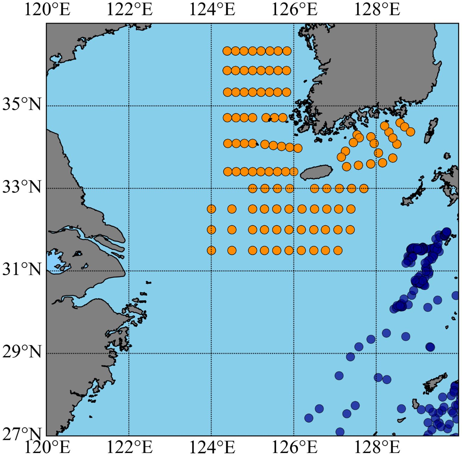
Figure 1. Locations of in-situ SSS measurements. NSO: orange points, Argo: blue points.

2.5 Data preprocessing

To develop the DNN SSS retrieval model, the following preprocessing was performed on all types of gridded data within the study area from 2016 to 2020. (1) Eliminate outliers in the SMAP Tb dataset affected by sea ice and sea spray based on the quality flags of L3 data. (2) Considering the different spatial resolutions of datasets from multiple sources, all datasets were spatiotemporally matched and then resampled onto a unified 0.25° grid using bilinear interpolation, enabling direct comparisons and analysis. (3) Grid points with an instantaneous rainfall rate exceeding 0.15 mm/h were excluded, since heavy rainfall significantly influences the brightness temperature observed by microwave radiometers. (4) Calculate the shortest offshore distance of grid points based on latitude and longitude. (5) Remove all NaN values. (6) Normalize the input values including Tb and environmental data to standardize the feature range by transforming the data to have a mean of 0 and a standard deviation of 1, which is a critical step in ensuring consistency across different datasets and preventing performance biases caused by varying input feature scales.

Finally, we obtained a total of 996,063 data samples. These data were divided into two parts: the data from 2016 to 2019 were utilized for training and validation, and that in 2020 were used as independent test set. To further evaluate the performance of the DNN framework, in-situ measurements were collocated with the model retrieval results and SMAP SSS products using strict temporal and spatial criteria. Specifically, we used a 12 h time window and a 25 km spatial search radius. This matching process results in a total of 1,540 collocated samples.

3 DNN based salinity retrieval model

3.1 Architecture of the deep neural network

The architecture of the DNN model (Yuan et al., 2020) for SSS retrieval is depicted in Figure 2, which consists of an input layer, three hidden layers, and an output layer. The performance of a DNN is significantly influenced by several factors, including the number of hidden layers, the number of neurons in each hidden layer, the learning rate, the choice of optimizer, and the activation function (Liu et al., 2017; Zhang et al., 2023). To identify the optimal set of network parameters, a series of sensitivity experiments were conducted by evaluating the model performance under various configurations: 1) The number of neurons in the three hidden layers was tested within the ranges of 64 to 1024, 32 to 256, and 32 to 128, for the first, second and third layers, respectively. 2) The batch size varied between 256 and 2048. 3) The learning rate was randomly sampled between 0.0001 and 0.01. 4) The dropout rate was set between 0 and 0.3. 5) The optimizers tested include SGD, RMSprop, and Adam, both with and without batch normalization.

Figure 2

Figure 2. The architecture of the DNN framework for SSS retrieval.

The network architecture uses the ReLU activation function and mean squared error (MSE) loss function. The remaining hyperparameters are optimized using a combination of grid search and random search. A total of 100 grid searches were performed, with an epoch setting of 500. The use of random search is specifically designed to efficiently explore the continuous hyperparameter space, particularly for parameters such as the learning rate by sampling values within a predefined interval rather than testing every discrete option in great detail through grid search. This approach, in combination with grid search, allows us to reduce computational costs while ensuring a comprehensive search for high-performance configurations. The results reveal that the optimal network parameters consist of 1024, 32, and 32 neurons, and dropout rates of 0.3, 0, and 0 for the three hidden layers, respectively, a batch size of 512, a learning rate of 0.008, and the Adam optimizer without batch normalization. Meanwhile, the DNN model was trained using K-Fold Cross Validation (Nti et al., 2021) to enhance its generalization ability.

3.2 Experimental design

During the development of the DNN model, the SHAP method (Lundberg and Lee, 2017) was employed to evaluate the relative importance of input parameters in SSS estimation. By calculating the Shapley value for each parameter, this approach effectively addresses the limitations of traditional feature importance methods, which often rely on linear assumptions. Specifically, the SHAP method is capable of accurately capturing the nonlinear interactions and coupling effects among multidimensional parameters.

We first conducted SHAP analysis for the entire study area and time period. As illustrated in Figure 3, the importance scores provide a clear representation of the contribution of each input parameter to the model performance. The significance of Tbv is evident, as it plays a pivotal role in revealing sea surface emissivity changes driven by salinity (Entekhabi et al., 2010). While the overall importance of Tbh is relatively low, possibly because it is generally less sensitive to SSS-induced emissivity changes than Tbv (Song and Wang, 2017). This may also explain why v-h ranks between Tbv and Tbh. But further analysis in different regions and seasons (Section 5) shows that the contribution of Tbh is more significant in offshore areas (50 km<dis ≤ 200 km) or in summer and autumn. Lat and lon rank among the top four, reflecting the spatial pattern in SSS, especially its more pronounced meridional gradient (Reul et al., 2014a). Theta also contributes a lot, which reflects the temporal variations of SSS to some extent. The overall importance of distance (dis) is relatively low, possibly because lat/lon features already implicitly contains distance information, thereby reducing the model’s need for explicit distance-based corrections. But it still shows greater impact in nearshore areas (dis<50 km) (Figure 4a), where freshwater input and land-sea interactions strongly affect salinity patterns. As for the environmental factors, the SHAP analysis results reveals the substantial contribution of SST, reflecting the thermodynamic interactions between temperature and salinity (Alory et al., 2012; Hernandez et al., 2014; Reul et al., 2014b; Umbert et al., 2015). However, the effects of wind speed and direction are much weaker, possibly because the linear combination of vertical and horizontal polarization brightness temperatures (v-h) introduced in this study already implies a relatively strong wind direction signal, and thus reduces the importance of wind-related information (Han and Hong, 2023; Soisuvarn et al., 2007). Rainfall exhibits a negligible effect, which should be due to the data preprocessing step excluding rain-contaminated data to mitigate the influence of RFI (Ouyang et al., 2023).

Figure 3

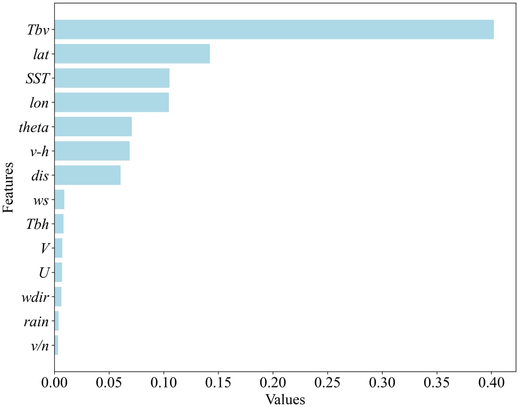
Figure 3. SHAP importance scores of input parameters in the baseline DNN model.

Figure 4

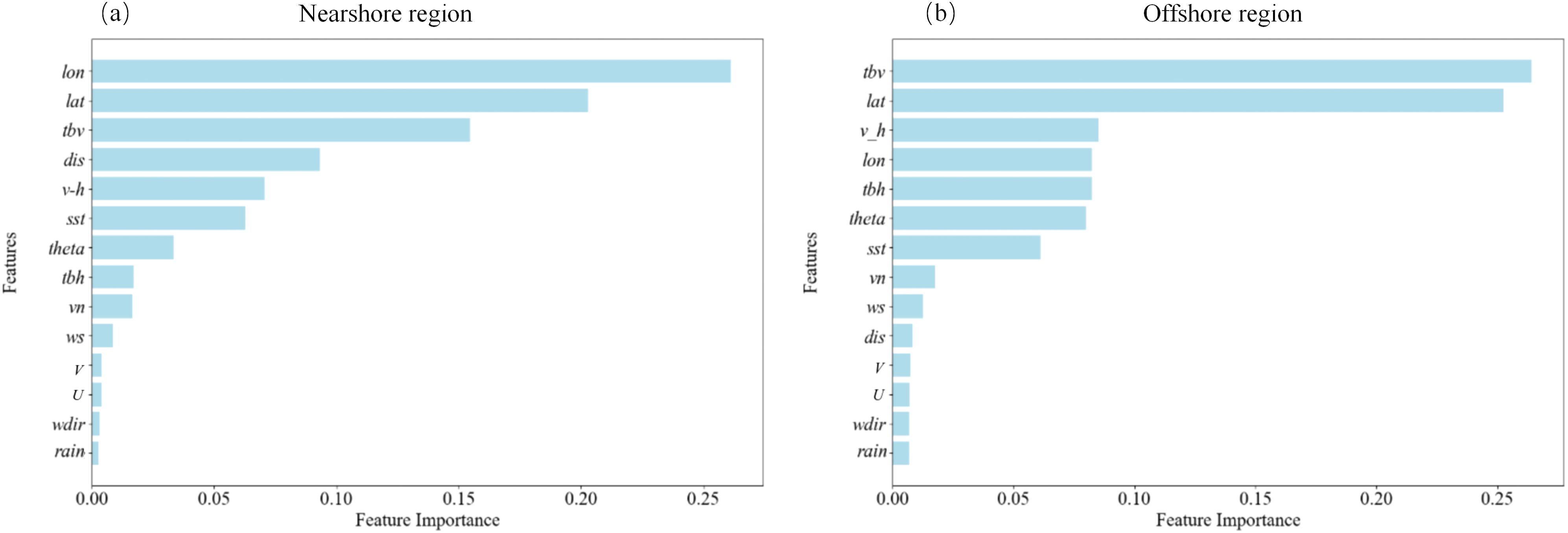
Figure 4. SHAP importance scores of input parameters in DNN-nearshore (a) and DNN-offshore (b) models.

Incorporating all parameters into DNN may lead to increased training time. Moreover, the inclusion of redundant information may potentially reduce the model performance. Based on the results of the SHAP analysis, this study designed a series of feature combination experiments to evaluate the cumulative effects of parameter contributions and identify the optimal set of input parameters. All sensitivity experiments were conducted throughout the entire study area and time period, using consistent three-layer DNN architecture based on the previously optimized network configuration, which ensures that any variations in performance could be attributed to differences in input parameters.

As presented in Table 1, the first stage involves the construction of four DNN models: 1) Model 1 (one parameter) uses only the primary feature Tbv as the control group. 2) Model 2 (two parameters) examines the impact of incorporating the marine environment factor, SST. 3) Model 3 (three parameters) assesses the spatial representation capability of geographic coordinates (lat and lon). 4) Model 4A or 4B (four parameters) further quantifies the combined effects of geographic coordinates and SST or dis, respectively. In the subsequent stages, from Model 5 to Model 9, the next most important parameter identified by the SHAP analysis was sequentially incorporated. This approach allows for a detailed evaluation of the incremental contributions of each parameter to model performance.

Table 1

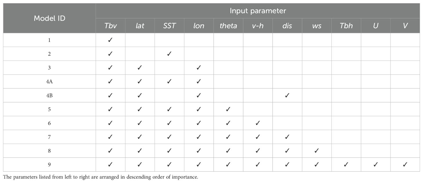
Table 1. Input parameter settings of the baseline DNN models.

The performance of the DNN model was evaluated using three key metrics: the RMSE, bias, and Pearson’s correlation coefficient (CORR). Additionally, to highlight the advantages of the DNN model, we further conducted comparative analysis with three other machine learning models, namely K-Nearest Neighbors (KNN) (Taunk et al., 2019), Random Forest (RF) (Breiman, 2001), and Extreme Gradient Boosting (XGBoost) (Chen and Guestrin, 2016).

4 Results

4.1 Determination of optimal model input parameters

Figure 5 illustrates the performance of each baseline DNN model listed in Table 1. The RMSE between model estimations and HYCOM values is 1.27 when using only Tbv as input in Model 1, indicating that the radiation signal from SMAP contains important information on sea surface salinity. Additional inclusion of SST in Model 2 improves model accuracy, albeit to a limited extent. However, the incorporation of latitude and longitude in Model 3 significantly reduces the RMSE by 33% and increases the CORR to 0.87. Comparing Models 4A and 4B with Model 3, further adding SST or dis exhibits a small contribution to model performance. This suggests that geographic information effectively reflects the inherent regional characteristic of SSS.

Figure 5

Figure 5. Performance of the DNN models 1–9 with different input parameters.

As the number of input parameters continues to increase, the accuracy of salinity estimation gradually improves. Model 7, which combines the first seven most important input parameters-Tbv, lat, SST, lon, theta, v-h, and dis, achieves the highest accuracy, with RMSE of 0.69, bias of -0.11 and CORR of 0.91. Further inclusion of wind speed (ws) information or Tbh in Models 8 and 9 produces salinity estimation results comparable to Model 7, indicating that high-accuracy SSS estimation can be achieved without inputting these parameters. This minimizes data redundancy while retaining the essential physical factors. The results also confirm the SHAP analysis findings that the contribution of wind or Tbh to the baseline DNN model is not significant. Consequently, the seven parameters in Model 7 were selected as the optimal input set. When comparing DNN with other machine learning models in the next section, all models use the same set of input parameters.

4.2 Overall performance of the DNN model

Table 2 shows the RMSE, bias and CORR values between HYCOM reanalysis and sea surface salinity derived from the baseline DNN, KNN, RF, and XGBoost models. To ensure optimal performance of each model, all models underwent hyperparameter optimization using grid search, with parameter spaces customized for each algorithm. Specifically, for RF and XGBoost, key parameters such as tree depths, feature selection methods, and sample splitting criteria were adjusted to enhance accuracy. For KNN, the number of neighbors, search algorithms, distance weighting method, and leaf size were optimized to ensure robust retrieval while balancing model complexity. In general, the independent validation using HYCOM data from 2021 demonstrates that RF, XGBoost, and DNN achieve comparable levels of high accuracy. These models significantly outperform KNN with RMSE approximately 17% lower.

Table 2

Table 2. Statistical errors between sea surface salinity derived from different machine learning models and HYCOM reanalysis data from 2021.

To further investigate the robustness of the models, we compared model estimations against in-situ measurements. The accuracy of SMAP salinity product was also evaluated based on the same dataset. As shown in Table 3 and Figure 6, when compared with in-situ observations, the tree-based models (RF and XGBoost) exhibit degraded performance and is inferior to that of the SMAP products, with the maximum RMSE value exceeding 1.05 and minimum CORR value dropping to 0.55. In contrast, the DNN model remains high performance. The RMSE is 0.78, which is 38.6% lower than that of XGBoost and also the lowest among all evaluated models. Compared to the SMAP products, the RMSE has decreased by 25.7%, further highlighting its superior performance.

Table 3

Table 3. Statistical errors between sea surface salinity derived from different machine learning models or SMAP products and in-situ measurements.

Figure 6

Figure 6. Scatter density plot of SMAP products (a) and model estimations (b-d) compared with in-situ sea surface salinity measurements. (b-d) denote RF, XGBoost and baseline DNN model results, respectively.

The DNN model’s enhanced performance can be attributed to its ability to learn hierarchical representations from SMAP brightness temperature and ancillary parameters, effectively capturing the non-linear interactions between oceanographic or geographic factors and salinity changes. Additionally, the DNN model achieves a CORR value of 0.78, slightly higher than that of the SMAP products, indicating a strong linear relationship with in-situ measurements. This reveals the high ability and robustness of the DNN model to learn complex feature interactions.

5 Discussion

Based on the above findings, we focused on discussing the performance of the optimal baseline DNN model in time and space in this section. All analyses were based on comparisons with independent in-situ measurements to further demonstrate the robustness of the model.

5.1 Model performance in nearshore and offshore regions

Table 4 compares DNN model estimation results and SMAP salinity products with in-situ measurements in the nearshore region less than 50 km away from land and offshore region 50 km to 200 km away from land, respectively. Obviously, the baseline DNN exhibits varying performance in different regions. In the nearshore region, compared to the SMAP products, the RMSE (0.88) of DNN derived SSS has significantly decreased by 33.8%. This indicates that the DNN model is more effective in capturing coastal salinity changes, where factors such as coastal processes and river runoff significantly affect the magnitude and spatiotemporal distribution of salinity. In this region, the relatively low accuracy of SMAP products is likely due to noise and interference from land-based sources.

Table 4

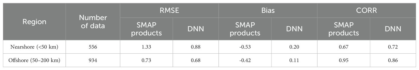
Table 4. Statistical errors of baseline DNN derived sea surface salinity and SMAP products against in-situ measurements in different regions.

In offshore areas, the accuracy of both DNN estimation and SMAP products has been greatly improved. Especially for the SMAP products, the RMSE has decreased from 1.33 in coastal areas to 0.73. On the one hand, the impact of RFI is much smaller here. On the other hand, the salinity patterns of offshore waters become more stable and consistent. Compared with the SMAP products, the DNN estimation still maintains slightly higher accuracy, which is likely due to its superior ability to learn and generalize complex patterns and relationships in data more effectively than traditional methods.

Due to the different characteristics of SSS in nearshore and nearshore regions, can we further improve the accuracy of salinity retrieval by establishing separate regional models? To address this issue, input parameter importance analysis and sensitivity experiments described in Section 3.2 were conducted in each region. As shown in the SHAP analysis results in Figure 4, key factors such as Tbv and geographic coordinates still maintain high importance scores in both regions, although their rankings are slightly different. Compared with Figure 3, the role of the distance is more prominent in nearshore areas, which may reflect the more significant impact of coastal processes on salinity and the complex interactions between land and sea. In offshore regions, its impact is greatly reduced, but subsequent sensitivity experiments show that incorporating it into the model input can substantially reduce salinity retrieval errors. In addition, Tbh emerges as an important factor in offshore areas. Based on these findings, optimal input parameters were determined through sensitivity assessment of nearshore and offshore DNN models. For DNN-nearshore, the optimal input parameters are the same as the baseline DNN model, i.e., Lon, Lat, Tbv, dis, v-h, SST and theta. When considering Tbh additionally, DNN-offshore demonstrates the best performance.

Figures 7, 8 compare the performance of the baseline DNN, DNN-nearshore and DNN-offshore models, as well as the quality of SMAP products in different regions. Overall, both two regional models outperform the baseline DNN in terms of RMSE and correlation coefficient. In the nearshore region, DNN-nearshore derived RMSE is reduced to 0.81, about 8.0% lower than that of baseline DNN, and the correlation coefficient increases by approximately 12.5% from 0.72 to 0.81. In offshore areas, DNN-nearshore achieves a RMSE of 0.64, 5.9% smaller than that of baseline DNN, and the correlation coefficient is as high as 0.90. On the contrary, the bias of the two regional models has increased, but still less than 0.3. These results demonstrate that regional modeling helps to further improve the accuracy of salinity retrieval. This may be attributed to the fact that the regional sample data more accurately reflect the spatiotemporal distribution characteristics of salinity in each area, allowing the model to focus more specifically on the unique data features.

Figure 7

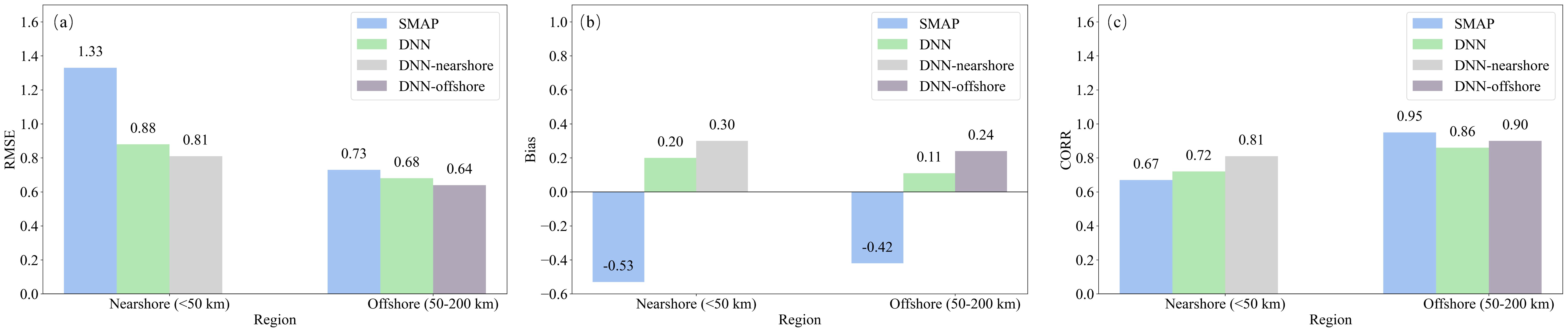
Figure 7. RMSE (a), bias (b) and CORR (c) of baseline DNN, DNN-nearshore and DNN-offshore derived SSS, and SMAP products against in-situ measurements.

Figure 8

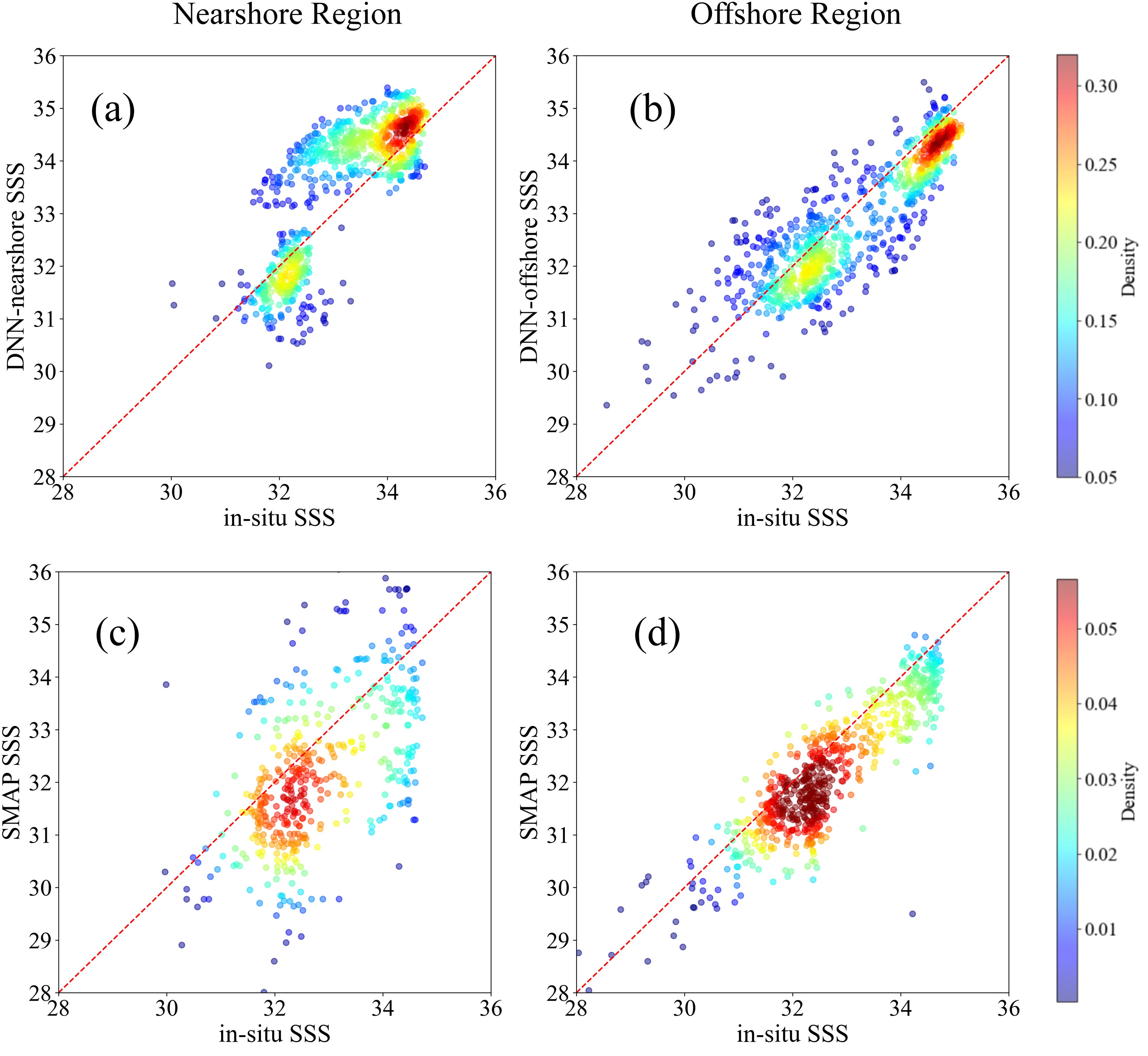
Figure 8. Comparison between DNN-nearshore and DNN-offshore derived salinity (a, b) and SMAP products (c, d) with in-situ measurements in the nearshore (left) and offshore regions (right).

5.2 Model performance in different seasons

This section further evaluates the robustness of two regional models by analyzing their performances in different seasons. As shown in Figure 9, the RMSE of both models and SMAP products show some seasonal variation, but the magnitude of change is much smaller in the offshore region, which may be related to the relatively more stable distribution of salinity in this area. In nearshore areas, compared to SMAP salinity products, DNN-nearshore significantly reduces salinity estimation error in each season, especially in spring and winter, with the RMSE 60.3% and 53.6% lower than that of SMAP products, respectively. In offshore, the model error shows a more stable seasonal variation trend, with values ranging from 0.5 and 0.7, also much smaller than that of SMAP products in spring and winter. This indicates that the regional salinity retrieval models can accurately capture changes in coastal salinity over time.

Figure 9

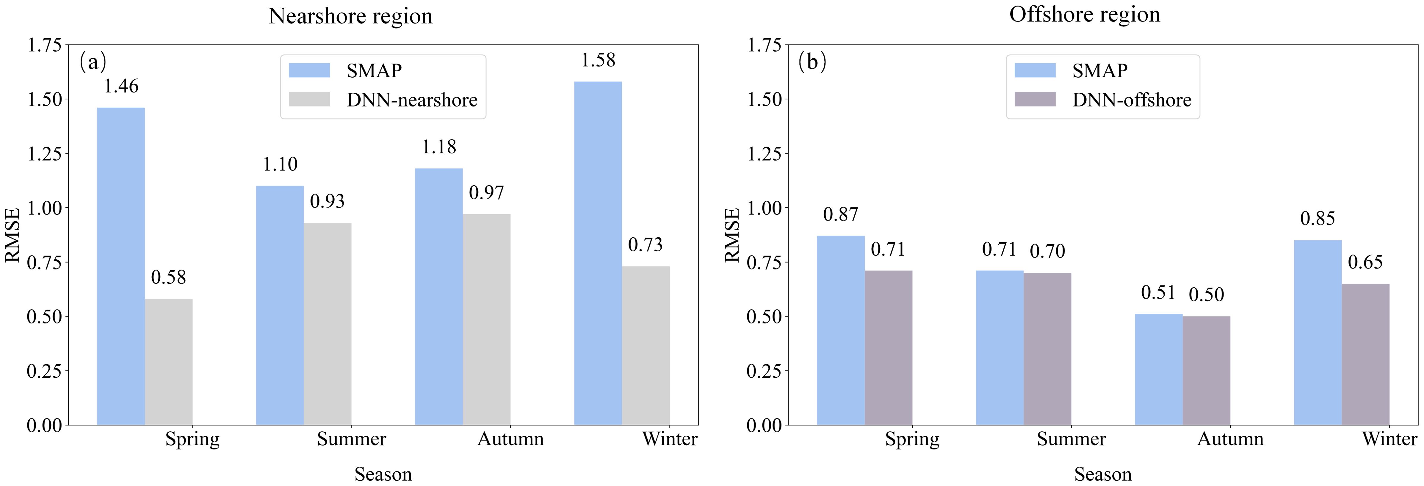
Figure 9. Seasonal variation of DNN-nearshore (a) and DNN-offshore (b) derived RMSE and SMAP products against in-situ measurements.

Considering that the performance of DNN-nearshore is slightly lower than that of DNN-offshore, and nearshore salinity often exhibits more pronounced seasonal variations due to the influence of dynamic processes or estuarine runoff. In nearshore areas, we attempt to investigate whether seasonal adaptive models can further improve salinity retrieval accuracy. SHAP analysis reveals that the top ten input parameters remain consistent across all four seasons, although their rankings vary slightly. Among them, Tbv and geographic information (lat and lon) consistently rank in the top four, highlighting their fundamental role in salinity retrieval, and dis remains a key parameter, reflecting its crucial impact on the spatial variation of nearshore salinity caused by land-sea interactions. In summer and autumn, the importance of Tbh rises, indicating an increased correlation with salinity during these periods, which may be due to seasonal fluctuations in ocean thermal characteristics and radiation signals. Sensitivity experiments further determine the optimal input parameters for each seasonal model (DNN-nearshore-season). During spring and winter, the selected input parameters align with those of DNN-nearshore or baseline DNN. In summer and autumn, the seasonal models incorporate one additional parameter Tbh.

Figure 10 compares the performance between four seasonal DNN models (DNN-nearshore-season) and the non-seasonal nearshore model (DNN-nearshore). The results reveal that accounting for seasonal variations significantly enhances salinity retrieval accuracy across all seasons. Compared to the non-seasonal DNN-nearshore model, the average RMSE is reduced by 12.3% from 0.81 to 0.71, and the most substantial improvements in accuracy appear in summer and autumn, with RMSE decreasing by 13% and 18%, respectively. This suggests that the seasonal modeling approach effectively captures temporal variations in the relationship between input parameters and nearshore salinity. By dynamically adjusting the weights of input features across different seasons, the DNN-nearshore-season models achieve superior performance, highlighting the importance of incorporating seasonal dynamics in salinity estimation.

Figure 10

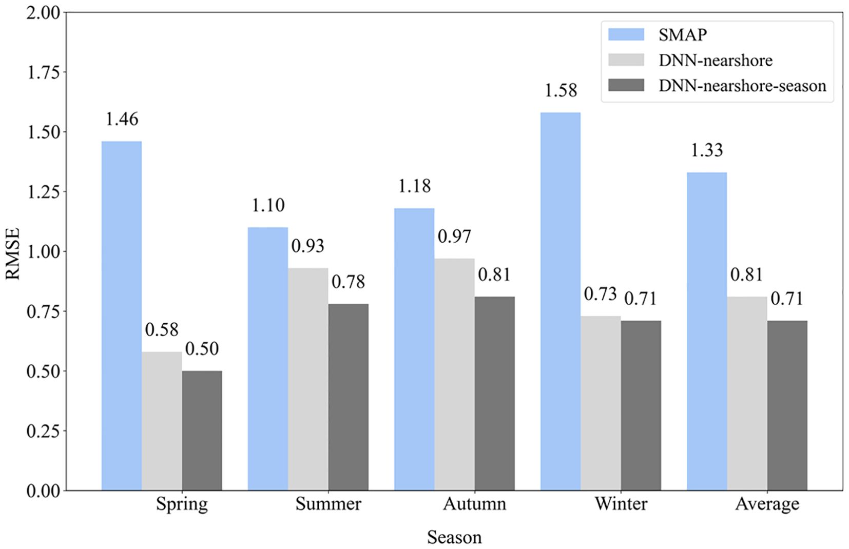
Figure 10. RMSE of DNN-nearshore and DNN-nearshore-season derived SSS, and SMAP products against in-situ measurements in the nearshore region.

6 Conclusion

In this study, we utilized DNN to construct sea surface salinity retrieval model in the Yellow and East China Seas based on HYCOM reanalysis data. This architecture established a standardized salinity retrieval framework characterized by operational simplicity and broad applicability across diverse marine environments. The results demonstrate that the DNN model exhibits remarkable robustness, primarily attributable to its capacity to extract useful information from extensive datasets and effectively incorporate multi-dimensional oceanographic and geographic variables.

SHAP analysis was employed to investigate contributions of various parameters (including SMAP observations, geographic and temporal information, and ocean and atmospheric variables) to model performance, followed by a series of sensitivity experiments to determine the optimal combination of input parameters and network configuration. It turns out that a combination of seven input parameters, including Tbv, lat, SST, lon, theta, v-h, dis, yielded the best performance for the baseline DNN model constructed for the entire study area and time period. Comparative analysis based on both HYCOM data and independent in-situ measurements shows that the optimal baseline DNN model has significant superiority over other machine learning methods such as KNN, XGBoost and RF models. Meanwhile, compared with SMAP salinity products, the baseline DNN also performs much better, with RMSE reductions of 33.8% and 7.3% in nearshore and offshore areas, respectively.

More importantly, our findings quantitatively reveal the necessity of implementing regional and seasonal modelling strategies for salinity estimation. Compared with the baseline DNN model, the accuracy of the regional DNN model was improved to varying degrees in both nearshore and nearshore areas. The seasonal DNN models in nearshore areas further improve the accuracy of salinity retrieval, particularly in summer and autumn, with RMSE decreased by 13% and 18%, respectively, compared to non-seasonal models. This indicates that spatiotemporal modeling method can effectively capture complex salinity variation patterns, particularly in challenging nearshore areas where traditional methods such as SMAP products exhibit larger errors.

Overall, this study demonstrates the significant advantages of the DNN framework in SSS retrieval tasks, especially in dynamically complex ocean environments. These findings indicate the potential of DNN in providing more accurate and reliable salinity measurements, which is of great significance for the study of oceanographic processes. Future research can explore the impacts of more environmental variables such as river runoff on salinity changes in coastal waters based on more higher-quality data, thereby further enhancing the performance and applicability of deep learning based salinity retrieval models.

Data availability statement

The raw data supporting the conclusions of this article will be made available by the authors, without undue reservation.

Author contributions

YW: Data curation, Writing – review & editing, Methodology, Writing – original draft, Visualization, Formal Analysis. QX: Methodology, Supervision, Writing – original draft, Investigation, Writing – review & editing. XY: Writing – review & editing, Formal Analysis, Visualization, Methodology, Data curation. YL: Data curation, Methodology, Writing – review & editing, Investigation. KF: Investigation, Writing – review & editing, Visualization, Methodology.

Funding

The author(s) declare that financial support was received for the research and/or publication of this article. This research was funded by the National Natural Science Foundation of China (Grant No. T2261149752, 42476172). Hainan Province Science and Technology Special Fund under Grant SOLZSKY2025010 and ZDYF2023GXJS151.

Conflict of interest

The authors declare that the research was conducted in the absence of any commercial or financial relationships that could be construed as a potential conflict of interest.

Generative AI statement

The author(s) declare that no Generative AI was used in the creation of this manuscript.

Publisher’s note

All claims expressed in this article are solely those of the authors and do not necessarily represent those of their affiliated organizations, or those of the publisher, the editors and the reviewers. Any product that may be evaluated in this article, or claim that may be made by its manufacturer, is not guaranteed or endorsed by the publisher.

References

Alory G., Maes C., Delcroix T., Reul N., and Illig S. (2012). Seasonal dynamics of sea surface salinity off Panama: The Far Eastern Pacific fresh pool. J. Geophys Res. 117, C04028. doi: 10.1029/2011JC007802

Crossref Full Text | Google Scholar

Ammar A., Labroue S., Obligis E., Mejia C., Thiria S., and Crepon M. (2006). “Sea surface salinity retrieval throughout a SMOS half-orbit using neural networks.” in Proceedings of the 2006 IEEE MicroRad. (San Juan, PR: IEEE), 103–108. doi: 10.1109/MICRAD.2006.1677071

Crossref Full Text | Google Scholar

Bao S., Wang H., Zhang R., Yan H., and Chen J. (2019). Comparison of satellite-derived sea surface salinity products from SMOS, aquarius, and SMAP. J. Geophys. Res.: Oceans. 124, 1932–1944. doi: 10.1029/2019JC014937

Crossref Full Text | Google Scholar

Breiman L. (2001). Random forests. Mach. Learn. 45, 5–32. doi: 10.1023/A:1010933404324

Crossref Full Text | Google Scholar

Canadian Meteorological Centre (CMC) (2017). GHRSST Level 4 CMC0.1deg Global Foundation Sea Surface Temperature Analysis (GDS version 2). (NOAA National Centers for Environmental Information). Available online at: https://www.ncei.noaa.gov/archive/accession/GHRSST-CMC0.1deg-CMC-L4-GLOB (Accessed January 24, 2024).

Google Scholar

Chen T. and Guestrin C. (2016). “XGBoost: A scalable tree boosting system.” in Proceedings of the 22nd ACM SIGKDD International Conference on Knowledge Discovery and Data Mining(KDD ’16). (New York, NY: Association for Computing Machinery), 785–794. doi: 10.1145/2939672.2939785

Crossref Full Text | Google Scholar

Cummings J. A. and Smedstad O. M. (2014). Ocean data impacts in global HYCOM. J. Atmospheric Oceanic Technol. 31, 1771–1791. doi: 10.1175/JTECH-D-14-00011.1

Crossref Full Text | Google Scholar

Dinnat E. P., Le Vine D. M., Boutin J., Meissner T., and Lagerloef G. (2019). Remote sensing of sea surface salinity: Comparison of satellite and in situ observations and impact of retrieval parameters. Remote Sens. 11, 750. doi: 10.3390/rs11070750

Crossref Full Text | Google Scholar

Dossa A. N., Alory G., Costa da Silva A., Dahunsi A. M., and Bertrand A. (2021). Global analysis of coastal gradients of sea surface salinity. Remote Sens. 13, 2507. doi: 10.3390/rs13132507

Crossref Full Text | Google Scholar

Entekhabi D., Njoku E. G., O’Neill P. E., Kellogg K. H., Crow W. T., Edelstein W. N., et al. (2010). The soil moisture active passive (SMAP) mission. Proc. IEEE 98, 704–716. doi: 10.1109/JPROC.2010.2043918

Crossref Full Text | Google Scholar

Font J., Boutin J., Reul N., Spurgeon P., Ballabrera-Poy J., Chuprin A., et al. (2012). SMOS first data analysis for sea surface salinity determination. Int. J. Remote Sens. 34, 3654–3670. doi: 10.1080/01431161.2012.716541

Crossref Full Text | Google Scholar

Gould W. J. and Cunningham S. A. (2021). Global-scale patterns of observed sea surface salinity intensified since the 1870s. Commun. Earth Environ. 2, 76. doi: 10.1038/s43247-021-00161-3

Crossref Full Text | Google Scholar

Han K. H. and Hong S. (2023). Ocean salinity retrieval and prediction for Soil Moisture Active Passive satellite using data-to-data translation. IEEE Trans. Geosci. Remote Sens. 61, 1–15. doi: 10.1109/TGRS.2023.3272677

Crossref Full Text | Google Scholar

Hernandez O., Boutin J., Kolodziejczyk N., Reverdin G., Martin N., Gaillard F., et al. (2014). SMOS salinity in the subtropical North Atlantic salinity maximum: 1. Comparison with Aquarius and in situ salinity. J. Geophys Res. Oceans. 119, 8878–8896. doi: 10.1002/2013JC009610

Crossref Full Text | Google Scholar

Jang E., Kim Y. J., Im J., Park Y. G., and Sung T. (2022). Global sea surface salinity via the synergistic use of SMAP satellite and HYCOM data based on machine learning. Remote Sens. Environ. 273, 112980. doi: 10.1016/j.rse.2022.112980

Crossref Full Text | Google Scholar

Kalu I., Ndehedehe C. E., Okwuashi O., and Eyoh A. E. (2021). Assessing freshwater changes over Southern and Central Africa, (2002–2017). Remote Sens. 13, 2543. doi: 10.3390/rs13132543

Crossref Full Text | Google Scholar

Kerr Y. H., Waldteufel P., Wigneron J. P., Delwart S., Cabot F., Boutin J., et al. (2010). The SMOS mission: New tool for monitoring key elements of the global water cycle. Proc. IEEE. 98, 666–687. doi: 10.1109/JPROC.2010.2043032

Crossref Full Text | Google Scholar

Kesavakumar B., Shanmugam P., and Venkatesan R. (2022). Enhanced sea surface salinity estimates using machine-learning algorithm with SMAP and high-resolution buoy data. IEEE Access. 10, 74304–74317. doi: 10.1109/ACCESS.2022.3189784

Crossref Full Text | Google Scholar

Lary D. J., Alavi A. H., Gandomi A. H., and Walker A. L. (2016). Machine learning in geosciences and remote sensing. Geosci. Front. 7, 3–10. doi: 10.1016/j.gsf.2015.07.003

Crossref Full Text | Google Scholar

Li Z., Liu Z., and Xing X. (2019). User Manual for Global Argo Observational Data Set (V3.0) (1997-2019) (Hangzhou: China Argo Real-time Data Center).

Google Scholar

Liu W., Wang Z., Liu X., Zeng N., Liu Y., and Alsaadi F. E. (2017). A survey of deep neural network architectures and their applications. Neurocomputing 234, 11–26. doi: 10.1016/j.neucom.2016.12.038

Crossref Full Text | Google Scholar

Lundberg S. and Lee S.-I. (2017). “A unified approach to interpreting model predictions.” in Proceedings of the 31st International onference on Neural Information Processing Systems (NIPS'17). (Red Hook, NY: Curran Associates Inc.), 4768–4777. doi: 10.48550/arXiv.1705.07874

Crossref Full Text | Google Scholar

Mears C., Lee T., Ricciardulli L., Wang X., and Wentz F. (2022). RSS Cross-Calibrated Multi-Platform (CCMP) 6-hourly ocean vector wind analysis on 0.25 deg grid, Version 3.0 (Santa Rosa, CA: Remote Sensing Systems). doi: 10.56236/RSS-uv6h30

Crossref Full Text | Google Scholar

Meissner T., Wentz F. J., and Le Vine D. M. (2018). The salinity retrieval algorithms for the NASA Aquarius Version 5 and SMAP Version 3 Releases. Remote Sens. 10, 112. doi: 10.3390/rs1007112

Crossref Full Text | Google Scholar

Menezes V. V. (2020). Statistical assessment of sea-surface salinity from SMAP: Arabian Sea, Bay of Bengal and a promising Red Sea application. Remote Sens. 12, 447. doi: 10.3390/rs12030447

Crossref Full Text | Google Scholar

Miller J. L. and Payne S. (2000). “Remote sensing of coastal salinity: naval needs and developing capability. IGARSS 2000,” in Proceedings of the 2000 IEEE International Geoscience and Remote Sensing Symposium (IGARSS 2000). (Honolulu, HI: IEEE), 6, 2534–2536. doi: 10.1109/IGARSS.2000.859631

Crossref Full Text | Google Scholar

Ning J., Xu Q., Zhang H., Wang T., and Fan K. (2019). Impact of cyclonic ocean eddies on upper ocean thermodynamic Response to Typhoon Soudelor. Remote Sens. 11, 938. doi: 10.3390/rs11080938

Crossref Full Text | Google Scholar

Nti I. K., Nyarko-Boateng O., and Aning J. (2021). Performance of machine learning algorithms with different K values in K-fold cross-validation. Int. J. Inf. Technol. Comput. Sci. 6, 61–71. doi: 10.5815/ijitcs.2021.06.05

Crossref Full Text | Google Scholar

Olmedo E., Turiel A., González-Gambau V., González-Haro C., García-Espriu A., Gabarró C., et al. (2022). Increasing stratification as observed by satellite sea surface salinity measurements. Sci. Rep. 12, 6279. doi: 10.1038/s41598-022-10265-1

PubMed Abstract | Crossref Full Text | Google Scholar

Ouyang Y., Zhang Y., Chi J., Sun Q., and Du Y. (2023). Deviations of satellite-measured sea surface salinity caused by environmental factors and their regional dependence. Remote Sens. Environ. 285, 113411. doi: 10.1016/j.rse.2022.113411

Crossref Full Text | Google Scholar

Rajabi-Kiasari S. and Hasanlou M. (2019). An efficient model for the prediction of SMAP sea surface salinity using machine learning approaches in the Persian Gulf. Int. J. Remote Sens. 41, 3221–3242. doi: 10.1080/01431161.2019.1701212

Crossref Full Text | Google Scholar

Reul N., Chapron B., Lee T., Donlon C., Boutin J., and Alory G. (2014a). Sea surface salinity structure of the meandering Gulf Stream revealed by SMOS sensor. Geophys. Res. Lett. 41, 3141–3148. doi: 10.1002/2014GL059215

Crossref Full Text | Google Scholar

Reul N., Fournier S., Boutin J., Hernandez O., Maes C., Chapron B., et al. (2014b). Sea surface salinity observations from space with the SMOS satellite: A New Means to Monitor the Marine Branch of the Water Cycle. Surv Geophys. 35, 681–722. doi: 10.1007/s10712-013-9244-0

Crossref Full Text | Google Scholar

Reul N., Grodsky S. A., Arias M., Boutin J., Catany R., Chapron B., et al. (2020). Sea surface salinity estimates from spaceborne L-band radiometers: An overview of the first decade of observation, (2010–2019). Remote Sens. Environ. 242, 111769. doi: 10.1016/j.rse.2020.111769

Crossref Full Text | Google Scholar

Reynolds R. W., Smith T. M., Liu C., Chelton D. B., Casey K. S., and Schlax M. G. (2007). Daily high-resolution-blended analyses for sea surface temperature. J. Climate. 20 (22), 5473–5496. doi: 10.1175/2007JCLI1824.1

Crossref Full Text | Google Scholar

Sam-Khaniani A. (2022). Evaluation of HYCOM sea surface salinity and temperature using buoy measurements. Earth Observation Geomatics Eng. 6, 38–48. doi: 10.22059/eoge.2023.355151.1131

Crossref Full Text | Google Scholar

Schmitt R. W. (2008). Salinity and the global water cycle. Oceanography 21, 12–19. doi: 10.5670/oceanog.2008.63

Crossref Full Text | Google Scholar

Soisuvarn S., Jelenak Z., and Jones L. (2007). An ocean surface wind vector model function for a spaceborne microwave radiometer. IEEE Trans. Geosci. Remote Sensing. 45, 3119–3130. doi: 10.1109/TGRS.2007.895418

Crossref Full Text | Google Scholar

Song Q. T. and Wang Z. H. (2017). Sea surface salinity observed from the HY-2A satellite. Satellite Oceanogr. Meteorol. . 2, 41–48. doi: 10.18063/SOM.2017.01.004

Crossref Full Text | Google Scholar

Song H., Zhang Y., Zhang B., Lv Y., and Zhang L. (2024). “Coastal regions sea surface salinity retrieval of SMAP mission based on light gradient boosting model,” in Photonics & Electromagnetics Research Symposium (PIERS). (Chengdu, China: IEEE), 1–3. doi: 10.1109/PIERS62282.2024.10618839

Crossref Full Text | Google Scholar

Stammer D., Martins M. S., Köhler J., and Köhl A. (2021). How well do we know ocean salinity and its changes? Prog. Oceanogr. 190, 102478. doi: 10.1016/j.pocean.2020.102478

Crossref Full Text | Google Scholar

Stolwijk A. M., Straatman H., and Zielhuis G. A. (1999). Studying seasonality by using sine and cosine functions in regression analysis. J. Epidemiol. Community Health 53, 235–238. doi: 10.1136/jech.53.4.235

PubMed Abstract | Crossref Full Text | Google Scholar

Tang W., Fore A., Yueh S., Lee T., Hayashi A., Sanchez-Franks A., et al. (2017). Validating SMAP SSS with in situ measurements. Remote Sens. Environ. 200, 326–340. doi: 10.1016/j.rse.2017.08.021

Crossref Full Text | Google Scholar

Tang W., Yueh S., Fore A., Vazquez-Cuervo J., Gentemann C., and Hayash A. (2022). “Assessment of SMAP SSS in coastal region using saildrones,” in Proceedings of the 2022 IEEE International Geoscience and Remote Sensing Symposium (IGARSS 2022), (Kuala Lumpur, Malaysia: IEEE), 6749–6752. doi: 10.1109/IGARSS46834.2022.9883972

Crossref Full Text | Google Scholar

Taunk K., De S., Verma S., and Swetapadma A. (2019). “A brief review of nearest neighbor algorithm for learning and classification,” In Proceedings of the 2019 International Conference on Intelligent Computing and Control Systems (ICCS), 1255–1260. Madurai, India: IEEE, 2019 doi: 10.1109/ICCS45141.2019.9065747

Crossref Full Text | Google Scholar

Umbert M., Guimbard S., Lagerloef G., Thompson L., Portabella M., Ballabrera-Poy J., et al. (2015). Detecting the surface salinity signature of Gulf Stream cold-core rings in Aquarius synergistic products. J. Geophys Res. Oceans. 120, 859–874. doi: 10.1002/2014JC010466

Crossref Full Text | Google Scholar

Wang H. and Li X. (2024). DeepBlue: Advanced convolutional neural network applications for ocean remote sensing. IEEE Geosci. Remote Sens. Mag. 12, 138–161. doi: 10.1109/MGRS.2023.3343623

Crossref Full Text | Google Scholar

Xie P., Joyce R., Wu S.-H., Yarosh Y., Sun F., and Lin R. (2019). NOAA CDR Program. NOAA Climate Data Record (CDR) of CPC Morphing Technique (CMORPH) High Resolution Global Precipitation Estimates, Version 1 (NOAA National Centers for Environmental Information). doi: 10.25921/w9va-q159

Crossref Full Text | Google Scholar

Yuan Q., Shen H., Li T., Li Z., Li S., Jiang Y., et al. (2020). Deep learning in environmental remote sensing: Achievements and challenges. Remote Sens. Environ. 241, 111716. doi: 10.1016/j.rse.2020.111716

Crossref Full Text | Google Scholar

Zhang X., Wu M., Han W., Bi L., Shang Y., and Yang Y. (2022). Sea surface salinity inversion model for Changjiang estuary and adjoining sea area with SMAP and MODIS data based on machine learning and preliminary application. Remote Sens. 14, 5358. doi: 10.3390/rs14215358

Crossref Full Text | Google Scholar

Zhang L., Zhang Y., and Yin X. (2023). Aquarius sea surface salinity retrieval in coastal regions based on deep neural networks. Remote Sens. Environ. 284, 113357. doi: 10.1016/j.rse.2022.113357

Crossref Full Text | Google Scholar