Floating debris dynamics in a tidal strait: transport and retention in Sundklakkstraumen, Lofoten

Understanding the transport and retention of floating plastic debris in fjords and coastal systems is essential for targeted mitigation strategies. This study investigates surface transport dynamics in Storvika and Sundklakkstraumen, a tidally energetic system in the Lofoten archipelago, Northern Norway. We combine GPS-tracked drifter observations with high-resolution 2D and 3D hydrodynamic modeling to assess how tidal forcing shapes transport pathways, convergence zones, and debris retention. Field deployments during spring and neap tides revealed strong contrasts in particle behavior, with spring tides promoting rapid flushing along energetic channels and neap tides supporting localized recirculation and short-term retention. The 3D model outperformed the 2D configuration in resolving sub-basin features, achieving skill scores of ss = 0.833 compared to 0.804, and reproducing trajectory structures with endpoint errors under 100 meters. Retention zones increased significantly during weaker tidal forcing relative to strong tidal forcing, with a 40% increase in attracting Lagrangian Coherent Structures and a 50% rise in domain-wide flush-out time. Residence time, revisit probability, and flow structure metrics consistently indicated higher retention during neap tide. Spatial diagnostics identified three possible accumulation hotspots, primarily active under neap conditions, accounting for over 40% of total residence time while occupying only ∼ 20% of the basin area. Low kinetic energy, reduced transport efficiency, and strongly attracting FTLE structures characterized these zones. The combined modeling–observation approach highlights the dominant role of the tidal phase in modulating short-term transport versus the temporary entrapment of debris. While the model excludes wind, waves, and high-frequency runoff events, the sheltered nature of the domain and minimal river influence limit their significance in this setting. This validated multi-diagnostic approach provides a transferable methodology for assessing retention in similarly complex coastal environments, supporting pollution mitigation, aquaculture planning, and operational forecasting efforts.

1 Introduction

Marine plastic pollution is a pervasive global environmental challenge, driven by the continued increase in annual plastic waste production (Lebreton and Andrady, 2019). Plastics persist in aquatic environments for centuries, causing significant ecological and socio-economic impacts (Thompson et al., 2009). Between 1990 and 2015, approximately 90 million tons of plastic waste entered the world’s oceans (Bellou et al., 2021). Plastic waste is widely distributed, reaching remote regions via ship leakage and large-scale oceanic currents (Van Sebille et al., 2012). Over time, plastics fragment into microplastics, which are found in various marine species consumed by humans, raising concerns about food safety and human health (Cózar et al., 2014).

Coastal regions are particularly vulnerable to plastic accumulation, as marine litter is transported and deposited by tides, currents, and meteorological forces. Clean-up initiatives aim to address this issue, but beaches often serve as transient reservoirs where plastics accumulate temporarily before being resuspended. Pawlowicz (2021) analyzed trajectories from a large number of GPS-tracked drifters in the Salish Sea and found that the drifters tended to ground soon after entering nearshore zones. They hypothesized that the drifter’s approach towards the shoreline was primarily controlled by ocean currents rather than direct wind or wave forcing and described this process as diffusive. Similarly, Adame et al. (2025) used high-resolution drift simulations along the Australian coast to show rapid beaching of marine plastics due to oceanic transport processes.

Understanding nearshore plastic transport dynamics is crucial for predicting debris pathways and developing effective mitigation strategies (Van Sebille et al., 2015). Coastal areas are key accumulation zones where local hydrodynamic structures strongly influence plastic retention. Identifying these retention mechanisms is essential for optimizing clean-up efforts and reducing the impact of plastic pollution in marine ecosystems (Haarr et al., 2024). Certain coastal sites exhibit prolonged retention of plastic debris, suggesting that geophysical factors such as local circulation patterns play a critical role in accumulation. Hydrodynamic ocean models are valuable tools for predicting transport pathways and supporting strategic cleanup operations.

Recent studies by Solbakken et al. (2022) and Haarr et al. (2024) investigated plastic retention at beaches in the Lofoten archipelago, Northern Norway, highlighting the presence of local recirculation features acting as small-scale retention traps. A summary of debris composition and potential sources observed at Storvika is provided in Appendix B. These studies recommend applying ocean models to understand plastic retention mechanisms and trace the origins of marine debris. Building on this, we implement a widely used coastal ocean model focused on the Lofoten region, with particular emphasis on resolving strong tidal currents (up to 2 ms⁻¹) that influence floating debris transport (see, e.g., Børve et al., 2021, 2025).

Global-scale modeling studies have identified coastal zones as key areas for plastic accumulation (Onink et al., 2021), yet these efforts often rely on coarse-resolution models that oversimplify critical processes such as beaching, shoreline retention, and nearshore transport (Hernandez et al., 2025). The transport dynamics of floating marine debris in coastal environments remain insufficiently understood, largely due to the geometric complexity and unresolved fine-scale processes that dominate in nearshore regions (Hernandez et al., 2024). High-resolution models are therefore essential for capturing the intricate bathymetry, sub-mesoscale vortices, and dispersive transport mechanisms that strongly influence particle drift and accumulation patterns (Saint-Amand et al., 2023; Ward et al., 2023).

In this study, we apply a high-resolution unstructured grid model (Ghaffari et al., 2019; Børve et al., 2025; Espenes et al., 2023) to resolve the flow field of a high-latitude fjord system in northern Norway. Focusing on a tidally energetic basin with previously documented plastic deposition (Solbakken et al., 2022; Haarr et al., 2024), we integrate model simulations with targeted field observations to assess the system’s capacity for debris retention. Two hydrodynamic configurations, a depth-integrated 2D barotropic model and a fully resolved 3D model, were developed and validated to simulate the dominant flow structures. These velocity fields were subsequently coupled with a Lagrangian particle tracking model to examine debris transport dynamics in the upper water column. The study introduces a multi-diagnostic approach that integrates field data, hydrodynamic modeling, and Lagrangian diagnostics to assess short-term retention processes. Sundklakkstraumen—a high-latitude tidal strait in Lofoten, northern Norway—serves as the focal site for applying the multi-diagnostic approach in a high-resolution, data-supported coastal setting. While tailored to this specific environment, the approach could be adapted for use in other coastal systems characterized by complex topography and energetic tidal forcing. By combining in situ measurements with dedicated numerical modeling, this study enhances our understanding of transport mechanisms in complex tidal fjord environments.

2 Materials and methods

2.1 Study area

The Lofoten–Vesterålen region is characterized by a complex hydrodynamic setting shaped by a mosaic of small islands, fjords, and narrow straits. Circulation is primarily governed by the interaction of the Norwegian Atlantic Current (NwAC) and the Norwegian Coastal Current (NCC) with steep seabed topography (Ghaffari et al., 2018; Mitchelson-Jacob and Sundby, 2001). While earlier studies suggested that outflow from Vestfjorden occurred mainly through its southern boundary (Vikebø et al., 2007; Opdal et al., 2008), more recent work highlights the role of narrow tidal straits and strong semi-diurnal tidal currents in modulating local flow and transport (Børve et al., 2021; Nøst and Børve, 2021; Børve et al., 2025).

These semi-diurnal tides, with a typical excursion of approximately 2 m, propagate northward through the archipelago and interact with topography to produce vigorous tidal waves, turbulence, and non-linear eddies (Moe et al., 2002; Kurogi and Hasumi, 2019). In narrow straits where current speeds exceed 2–3 ms⁻¹, such interactions give rise to rectified tidal currents and net tracer transport via mechanisms such as tidal pumping—where flow separation forms self-propagating dipoles during outflow—and tidal rectification, driven by vortex stretching around islands and slopes (Børve et al., 2021; Moe et al., 2002; Benjamins et al., 2015). These processes play a key role in connecting Vestfjorden to the outer shelf and strongly influence local retention and exchange dynamics.

This study examines Sundklakkstraumen (Figure 1), one of the straits linking Vestfjorden and the Norwegian Sea. The bathymetry of this region is highly complex, characterized by shallow depths, submerged ridges, and varying channel widths that influence flow pathways. Sundklakkstraumen reaches a minimum depth of approximately 2 meters at the lowest astronomical tide and stretches 13 km in a southeast-to-northwest orientation. At its southern end, it connects to Gimsøystraumen, while its northern terminus opens into the Norwegian Sea. The width of the strait varies significantly, with a 260-meter span at the Sundklakkstraumen Bridge narrowing further in its central section, where multiple small islands divide the flow into three distinct channels with widths ranging from 20 to 50 meters. North of these islands, the channel widens to approximately 2 km.

Figure 1

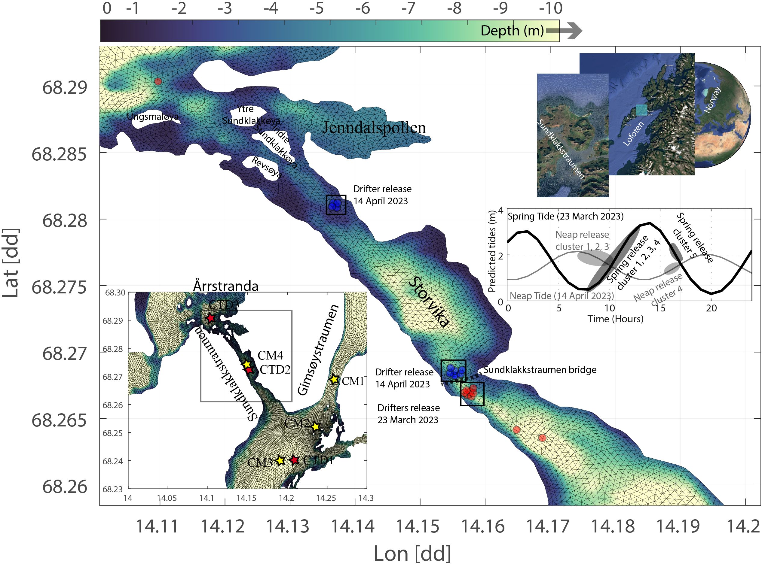
Figure 1. The study area in the Lofoten archipelago, Northern Norway, shows the bathymetry, unstructured model grid, and key observational and experimental locations. The main panel highlights the semi-enclosed Storvika basin and its connection to Sundklakkstraumen, with drifter release locations for both spring (March 23, 2023) and neap (April 14, 2023) tide experiments marked. The small right panel presents a time series of predicted tidal elevation, indicating the exact timing of drifter releases relative to tidal conditions. The inset map (bottom left) provides a broader view of the region, marking locations of current meters (CM1-CM4) and CTD stations used for model validation. Bathymetry is represented by color shading, with shallower areas in lighter tones and deeper regions in darker tones. A complementary figure is provided in Appendix D.

The role of these straits in marine debris transport has been previously investigated in studies such as Solbakken et al. (2022); Haarr et al. (2024), which examined the biweekly retention and deposition of beach litter at Storvika Bay, a site located along the northern coastline of a semi-enclosed bay within Sundklakkstraumen. These studies suggest that Storvika regularly receives fresh marine debris but may also function as a temporary retention site for floating litter. Plastic particles appear to be intermittently deposited and resuspended by hydrodynamic forces before eventually being advected away by currents or permanently beached. Both regional (matching general patterns across sites in the Lofoten archipelago) and highly local (distinguishing Storvika from other nearby locations within ∼ 10 km) sources of marine debris were identified. Consequently, the dynamics of beach litter in Storvika indicate that Sundklakkstraumen represents a compelling case study of the complex processes governing floating marine debris in nearshore waters, including continuous (though temporally variable) litter influx, resuspension and removal of previously beached material, and potential local retention of floating plastic particles.

2.2 Observations

Observations of near-surface currents were conducted using custom-designed GPS drifters to characterize micro- to mesoscale flow patterns and assess the influence of local bathymetry on transport dynamics. The drifters were adapted from CODE surface and MD03i designs (Davis, 1985; Callies et al., 2017), and modified for conditions specific to the study area. Each GPS-tracked surface drifter was custom-designed for current-following behavior and near-surface tracking, with a sampling frequency of 0.5 Hz. A detailed description and images of the instrument design and deployment are provided in Appendix A.

Two field campaigns were conducted on March 23, 2023 (spring tide) and April 14, 2023 (neap tide). The late-winter period was selected to isolate tidally driven transport processes under conditions of minimal freshwater discharge. Moreover, the Sundklakkstraumen channel is well-sheltered by surrounding topography, minimizing direct wind exposure. Consequently, wind and wave influences were considered negligible during both deployments.

A total of 24 unique GPS-enabled drifters were deployed across the two field surveys: 11 units during the spring tide campaign (March 23, 2023) and 13 during the neap tide campaign (April 14, 2023). Individual drifter releases were conducted using a time-staggered cluster strategy to span different tidal phases. Most deployments originated from the southern entrance of Storvika, using the Sundklakkstraumen bridge as a fixed vantage point. During the spring tide experiment, five clusters were released: Clusters 1 through 4 were deployed along the falling limb (ebb tide), and Cluster 5 was deployed during the rising limb (flood tide) to capture the flow reversal. A similar schedule was followed during the neap tide campaign, covering both ebb and flood phases. In addition, one cluster of four drifters was released at the northwestern entrance of the basin to evaluate lateral inflow and retention behavior under weaker tidal forcing.

Drift durations varied depending on tidal phase, grounding, and technical performance. Most drifters remained active between 6 and 12 hours, with typical trajectories lasting around 8 − 9 hours. A few units recorded shorter tracks (1 − 2 hours) due to early grounding or GPS dropout. The full drift duration range was 6−10.2 hours for the spring tide and 1−12.9 hours for the neap tide. These values align well with the 12-hour simulation periods used in the particle tracking experiments, ensuring adequate temporal coverage of both ebb and flood phases (see Appendix A).

During the spring tide campaign, three drifters required redeployment due to grounding or entanglement with sea ice. Usable trajectory data were retrieved from approximately 67% of spring tide drifters and 94% of neap tide drifters. Most data losses were attributed to GPS malfunction, such as non-recording or early cessation of positional logging. Despite these losses, the dataset yielded high-resolution trajectories that captured key tidal phases, supporting robust model validation and quantitative analysis of transport pathways.

2.3 Ocean model

We used the Finite Volume Community Ocean Model (FVCOM) (Chen et al., 2003), a prognostic, free surface, three-dimensional primitive equation model, to simulate drift dynamics in the Lofoten archipelago. The model employs unstructured triangular grids for detailed representation of narrow straits and complex bathymetry. Momentum advection is solved with a second-order flux scheme (Chen et al., 2006; Kobayashi et al., 1999), and horizontal diffusion is handled using the Smagorinsky (1963) closure scheme. Bottom friction is represented by a quadratic drag law:

$\begin{array}{ll}({\tau }_{b,x},{\tau }_{b,y})={\rho }_0{C}_d\left|\overrightarrow{u}\right|\overrightarrow{u},& (1)\end{array}$

where in Equation 1 C_d is the drag coefficient, ρ₀ is the reference seawater density, and $\overrightarrow{u}$ the velocity vector. In the 2D model, C_d follows the Chézy-Manning relation, which is provided in Equation 2:

$\begin{array}{ll}{C}_d=g\frac{n^2}{\sqrt[3]{D}},& (2)\end{array}$

with g gravitational acceleration, n the Manning coefficient, and D water depth. A Manning coefficient of n = 0.02 was selected based on validation against observations (Section 2.6; Børve et al. (2025)). In the 3D setup, bottom drag is calculated using a logarithmic law-of-the-wall formulation. The model equations were integrated using a modified explicit fourth-order Runge-Kutta scheme (Chen et al., 2003).

The model grid, adapted from Ghaffari et al. (2019), covers Nordland and southern Troms counties, extending into the Lofoten Basin. The horizontal resolution was 30−50 meters along coastlines and narrow straits, with refinement to 17 meters in Gimsøystraumen and Sundklakkstraumen (Figure 1) (Lynge et al., 2010; Børve et al., 2021). The 3D model incorporated realistic atmospheric forcing from AROME-Arctic (Müller et al., 2017) and open boundary conditions from ROMS (Röhrs et al., 2018). Freshwater input was provided by river discharge data from NVE (Ghaffari et al., 2019), supplemented with climatology-based synthetic data where real-time observations were unavailable (Beldring et al., 2003). The model ran from December 2022 to June 2023, with a three-month spin-up period to reach equilibrium before drift simulations. The external barotropic time step was set to 0.1 s, and the internal baroclinic time step was 0.8 s, based on a mode-splitting factor of 8, to ensure numerical stability in high-resolution coastal zones.

2.4 Drift model

We employed the open-source, Python-based Lagrangian framework OpenDrift (Dagestad et al., 2018, 2016), which is widely used for simulating passive particle advection in oceanic and atmospheric flows. Its modular design supports diverse applications, including oil spill tracking, ecological studies, and search and-rescue operations (Dagestad et al., 2018). For this study, we used the basic advection module assuming passive transport, omitting wind drag and Stokes drift, consistent with current-dominated conditions (Van Sebille et al., 2018).

Particle movement was computed by identifying the nearest horizontal grid cell, followed by vertical and temporal linear interpolation of velocity fields. Land boundaries were defined by the solid boundaries of the ocean model. Particles crossing the solid boundaries were returned to their last valid ocean position to avoid unrealistic accumulation.

Fjords are characterized by complex circulation patterns that include sub-mesoscale processes and residual currents, which can significantly influence particle retention (Bianucci et al., 2024). To assess transport and retention within the fjord-channel system, we integrated OpenDrift with 2D and 3D configurations of our hydrodynamic model. The simulations used idealized digital drifters deployed at 2 meters depth, aligned with the spatial and temporal release patterns of the field drifters, allowing for direct comparison with observed trajectories. This approach aligns with recent validation efforts employing GPS-tracked drifters to evaluate hydrodynamic model performance (Hunter et al., 2022).

Each experiment simulated 12 hours, covering the entire duration of field deployments. Particle depth was held constant, allowing 3D velocity gradients to influence horizontal drift, a method consistent with previous studies on Lagrangian coherence and subsurface transport (Jalón-Rojas et al., 2024).

2.5 Trajectory analysis

The drift model provides time-resolved particle trajectories, tracking where N particles are advected by the simulated ocean circulation throughout the study period. To extract meaningful retention and transport patterns from these trajectories, we applied a set of post-processing diagnostics, including Lagrangian Coherent Structures (LCS), residence time analysis, and revisit probability fields.

Lagrangian Coherent Structures were derived from Finite-Time Lyapunov Exponent (FTLE) fields, which reveal dynamically significant material surfaces acting as transient attractors or repellers in the flow field (Haller, 2015; Peacock and Haller, 2013; Shadden et al., 2005; Lekien and Ross, 2010; Serra et al., 2017; Leonard and Lucas, 2020). Particle trajectories were integrated using a fourth-order Runge–Kutta scheme, applied to surface-layer velocities from the high-resolution hydrodynamic model. The velocity field was interpolated onto a uniform 2 m grid, with linear spatial and temporal interpolation between hourly model outputs and particle positions updated every second (Δt = 1 s). Domain boundaries were treated with reflective conditions following Coulliette and Wiggins (2001); Beron-Vera et al. (2013). The FTLE field was computed as:

$\begin{array}{ll}\sigma (x_0,t_0,\tau )=\frac{1}{\left|\tau \right|}\text{ln }\left(\sqrt{{\text{λ}}_{\text{max}}(C(x_0,t_0,\tau ))}\right),& (3)\end{array}$

where in Equation 3 λ_max denotes the largest eigenvalue of the Cauchy–Green deformation tensor C, evaluated from the flow map gradient over the time interval τ. High FTLE values correspond to regions of rapid particle separation (repelling LCS), while strongly negative FTLE values indicate particle convergence (attracting LCS).

While FTLE-based LCS analysis provides information on coherent transport structures, it does not directly quantify particle residence time, which is critical for understanding debris accumulation. Therefore, we complemented the LCS results with residence time and revisit probability diagnostics. To achieve this, we divided the domain into a uniform 25 × 25 m grid and released one synthetic particle per cell per hour across full tidal cycles. Particle trajectories were integrated using a 1-second time step, with advection terminated upon exiting the model domain.

The total residence time in grid cell (i,j) was computed as:

$\begin{array}{ll}{T}_{i,j}={\displaystyle \sum _{t=1}^{N_t}{\displaystyle \sum _{p=1}^{N_p}{\delta }_{p,i,j}(t)·\text{Δ}t,}}& (4)\end{array}$

where ${\delta }_{p,i,j}(t)=1$ if particle $p$ occupies cell $(i,j)$ at time $t$, and $\text{Δ}t=1 \text{s}$.

The mean residence time per cell using Equation 4 is then defined as:

$\begin{array}{ll}{\overline{T}}_{i,j}=\frac{T_{i,j}}{V_{i,j}},\text{\hspace{1em}where\hspace{1em}}{V}_{i,j}={\displaystyle \sum _{t=1}^{N_t}{\displaystyle \sum _{p=1}^{N_p}{\delta }_{p,i,j}(t),}}& (5)\end{array}$

and V_i,j in Equation 5 denotes the total number of particle visits to cell (i,j).

Particle positions were updated according to:

$\begin{array}{ll}{x}_{p,i,j}(t+\text{Δ}t)=x_{p,i,j}(t)+u_{i,j}(t)·\text{Δ}t,& (6)\end{array}$

where x_p,i,j(t) is the particle position and u_i,j(t) is the interpolated velocity vector.

To further characterize spatial retention, we computed a revisit factor defined as the ratio of total particle visits, derived from Equations 5, 6, to the number of unique particles visiting each cell. This metric highlights zones of repeated re-entry and potential recirculation, offering additional insight into debris-trapping behavior within the domain.

2.6 Ocean model validation

Model validation was carried out using observational data from multiple sources to assess the accuracy of the hydrodynamic simulations. This includes profiling stations from the Sundklakkstraumen system, at the southern and northern ends of the channel, and centrally located in the basin, as shown in Figure 1, which provided vertical profiles of temperature, salinity, and velocity, offering comprehensive spatial coverage of the study domain. Additional long-term and multi-depth velocity data (at 5 m and 15 m depths over four months from March to June 2023) from Malnesfjord (14.593°E, 68.793°N), a nearby fjord with similar dynamic conditions, were used for a simplified multi-depth validation that aligns with methodologies employed in Norwegian fjord systems (Dalsøren et al., 2020; Kristensen and Gusdal, 2021).

Comparison between observed and simulated temperature and salinity profiles (Appendix C) demonstrated good agreement, despite a slight positive bias in both variables. This overestimation did not substantially affect transport predictions, given that the barotropic character of the system, rather than vertical stratification, dominates flow behavior. Recent studies emphasize that barotropic dominance is typical in fjords with strong tidal forcing (Cowton et al., 2015; Dalsøren et al., 2020), and resolving barotropic currents and sub-mesoscale features is essential for accurately modeling particle transport and retention in similar environments (Hecht and Hasumi, 2013; Fox-Kemper et al., 2011; McWilliams, 2016).

Velocity validation was the primary focus and showed high model fidelity. As illustrated in Figure 2, modeled current speeds at both 5 m and 15 m depths in CM1-CM4 displayed a strong correlation with observations. Linear regression lines for each depth closely followed the 1:1 relationship, with only minor deviations. The model underestimates the peak velocities (∼ 10%) in surface layers (5 m), which mirrors challenges reported in Norwegian Coast (NorKyst) operational model validations, where resolution limits and parameterized friction effects require careful calibration (Kristensen and Gusdal, 2021). One possible improvement could involve adjusting the Manning coefficient, which influences bottom friction and has been shown in previous sensitivity analyses to impact velocity magnitudes (Xie et al., 2022). Despite this minor underestimation, the validation results confirm the model’s robustness and reliability in simulating the hydrodynamic conditions of the Lofoten archipelago. The model successfully captured key velocity structures and spatial flow variations, providing a strong foundation for subsequent analyses of passive particle transport in the region. Similar model setups have also been validated against other regional observations, confirming their robustness (Børve et al., 2021, 2025).

Figure 2

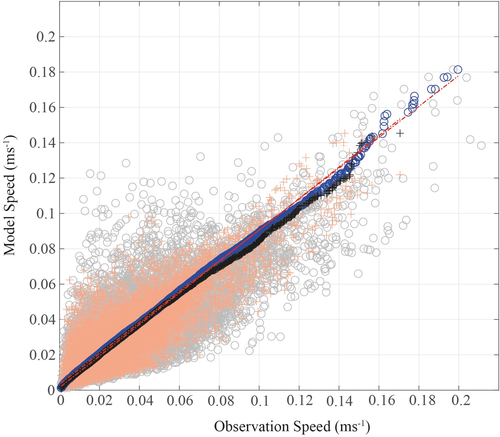
Figure 2. Comparison of 3D modeled current speeds with four months of current meter observations (March–June 2023) at stations CM1-CM4 in the Lofoten region. Observed and modeled data are partitioned by depth: 5 meters (gray circles) and 15 meters (red pluses). The corresponding regression fits for each depth are shown as blue circles (5 m) and black pluses (15 m). Red dashed lines represent the fitted regression lines for both depth levels.

3 Results and discussion

3.1 Flow dynamics

Figure 3 presents snapshots of the one-day maximum modeled flow speed at a depth of 1 meter from both the 3D (left panel) and 2D (right panel) simulations for the first field day, March 23^rd. The flow fields exhibit strong similarities, emphasizing the dominance of tidally driven currents in the region. These currents form coherent, linear jets that extend from narrow straits into the adjacent basin—an expected pattern given the region’s dynamic tidal forcing (Børve et al., 2021). The 3D simulation shows slightly higher surface-layer velocities compared to the 2D model, a difference attributed to its ability to resolve vertical structure and reduce the smoothing effects of depth-averaging. In contrast, the 2D model simplifies the velocity field by averaging over the water column, which can underestimate near-surface flow intensity.

Figure 3

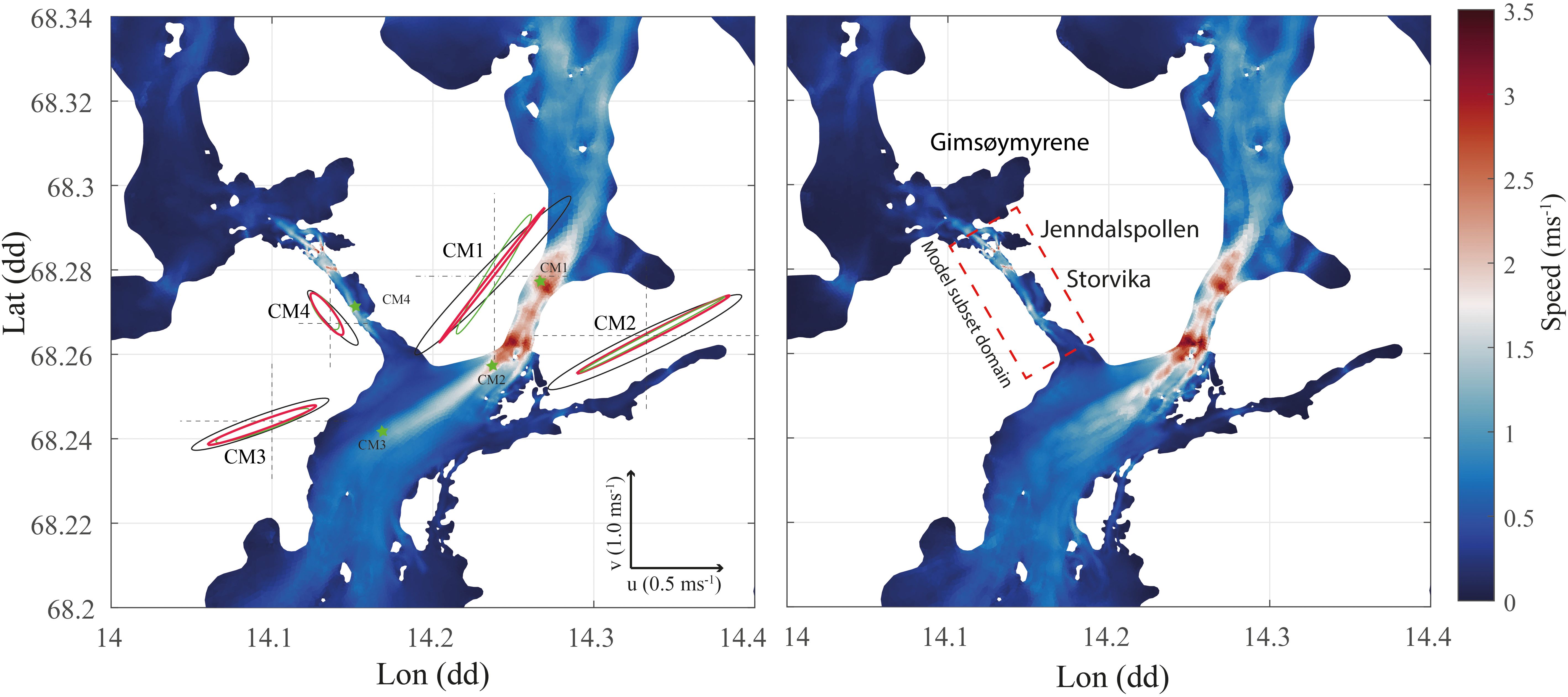
Figure 3. Modeled speeds utilized for synthetic drifter advection. The left-hand panel depicts the maximum speed at 1-meter depth in March 23^rd in the full 3D model. Surface, bottom, and depth-averaged current variance ellipses for four representative positions are denoted by black, green, and red colors, respectively. The right-hand panel displays the maximum speed on the same day derived from the barotropic tidal model.

Variance ellipses are widely used to represent the dominant direction and variability of horizontal current flow over time, with the major axis indicating the primary direction and magnitude of variability, and the minor axis reflecting cross-directional variability. Anisotropic (elongated) ellipses indicate strong directional flow, often aligned with topography (topographic steering and bathymetric alignment) or mean flow features, while isotropic (circular) ellipses indicate more uniform variability (Lumpkin and Johnson, 2013; Le Traon and Morrow, 2001; Elipot and Beal, 2015). In this study, ellipses were computed from a six-month 3D simulation to assess spatial coherence and the barotropic nature of the flow field. The results show that the major axes of the ellipses align closely with the geometry of the straits, confirming strong topographic control on flow direction. As further evidence, model diagnostics summarized in Table 1 indicate minimal vertical deviation in ellipse orientation across surface, bottom, and depth-averaged currents (≤ 3.5%), supporting the conclusion that baroclinic contributions to velocity are small (Kontogiannis and Bakas, 2020). However, during the summer months, stratification may enhance vertical shear and increase baroclinic effects (Lynge et al., 2010; Jing et al., 2025).

Table 1

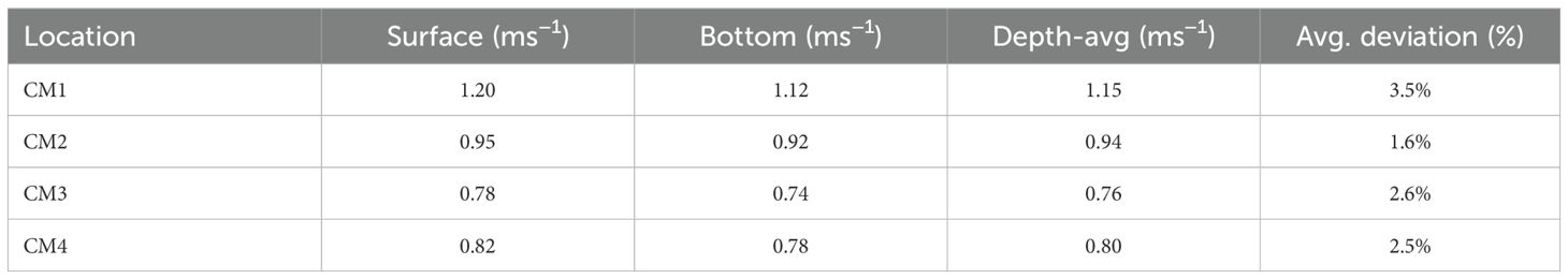
Table 1. Variance ellipse characteristics for surface, bottom, and depth-averaged currents at four locations.

To quantify the contribution of the barotropic mode to the overall flow dynamics, we calculated the fraction of energy associated with the depth-independent mode at these specified locations (Ghaffari et al., 2013). The energy fraction, R, is defined as:

$\begin{array}{ll}R=H\langle {\overline{u}}^2\rangle /\left[H\langle {\overline{u}}^2\rangle +{\displaystyle \langle {\int }_{\text{bott}}^{\text{surf}}{(u^{\prime })}^{2}dz\rangle } \right],& (7)\end{array}$

where in Equation 7 H is the depth, $\overline{u}$ and $u^{\prime }$ are the depth-averaged and depth-varying components of the flow field, respectively. The angle brackets indicate time-averaged values. The analysis revealed that approximately 70% of the total flow field variance across all selected positions is attributed to the barotropic mode, consistent with studies emphasizing tidal rectification in narrow channels (de Swart and Yuan, 2019; Zimmerman, 1980; Børve et al., 2021, 2025).

Storvika emerges as a site of particular interest due to its potential role as a transient collector and reservoir of floating marine debris (Haarr et al., 2024; Solbakken et al., 2022). Flow field analysis reveals that Storvika experiences markedly lower current velocities relative to more dynamic regions such as Gimsøystraumen. Within Storvika, peak velocities reach approximately 1 ms⁻¹ along the main channel adjacent to the southern shoreline, while the northern sector is characterized by substantially weaker flows, typically around 0.1 ms⁻¹. These reduced velocities along the northern coast suggest the presence of a sheltered and shallow zone that may act as a temporary hotspot for marine debris accumulation if particles enter the bay.

Nevertheless, the overall energy levels in the Storvika basin are higher than those observed in nearby semi-enclosed bays such as Jenndalspollen and Gimsøymyrene, which may offer more suitable conditions for long-term retention. As such, while Storvika may intermittently function as a debris accumulation zone, resuspension and redistribution are likely, particularly under spring tidal conditions when time-mean transport intensifies by approximately 20% compared to neap tide.

3.2 Drifter pathways

Figure 4 presents an overview of the trajectories of drifters released during both spring (left panels) and neap (right panels) tide phases, as observed in the field (top panels) and simulated using the 2D (middle panels) and 3D (lower panels) hydrodynamic models. These trajectories reveal clear contrasts between tidal phases, underscoring the dynamic interplay between tidal forcing and local bathymetry in shaping transport pathways in the Storvika–Sundklakkstraumen system.

Figure 4

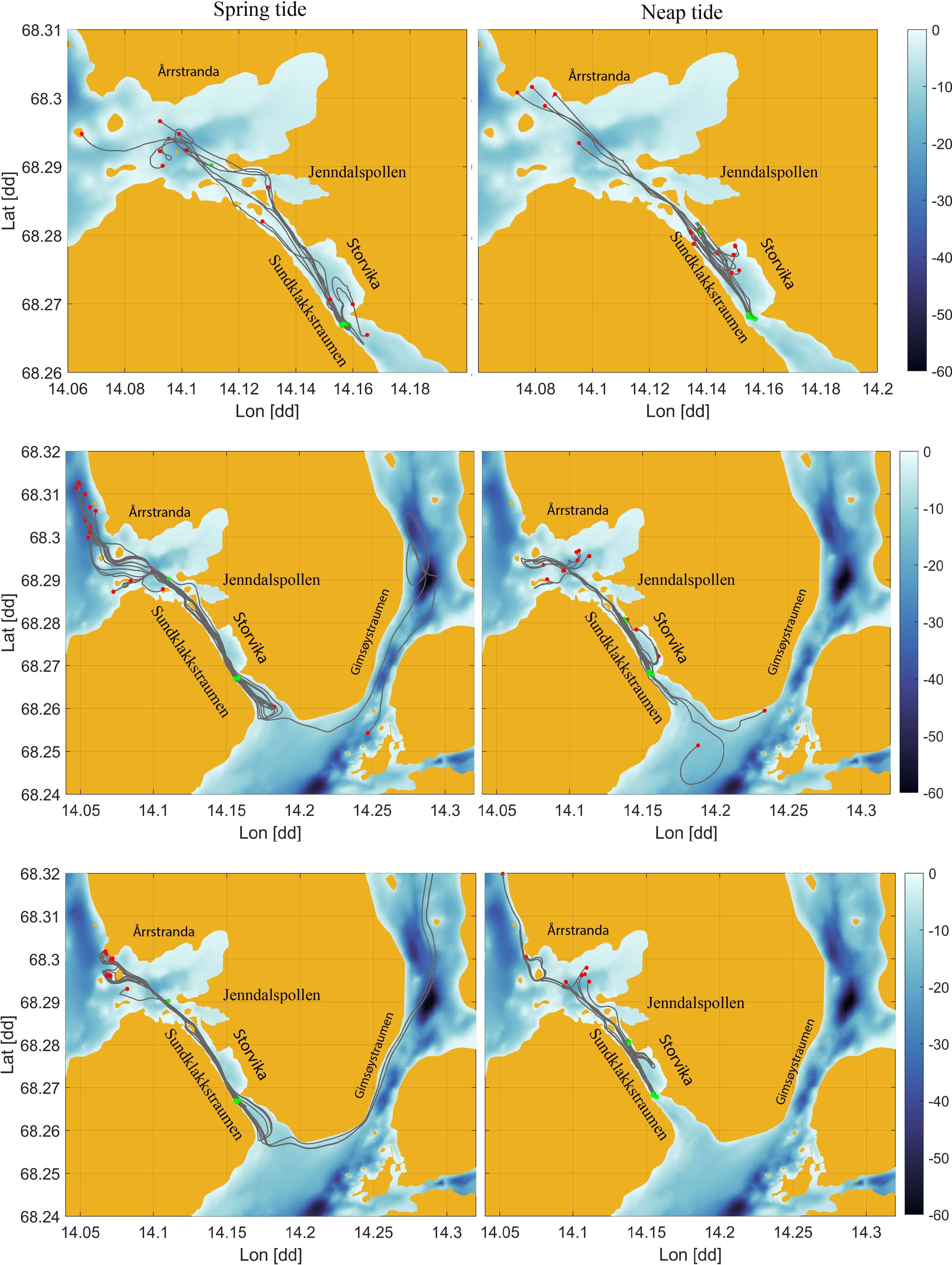
Figure 4. Drifter trajectories during spring and neap tides. The upper panels show the observed trajectories of drifters from the field campaigns conducted on March 23^rd (spring tide) and April 14^th (neap tide). The middle and lower panels display the corresponding simulated trajectories using the 2D and 3D hydrodynamic models. The color gradients in the background represent the bathymetry.

During spring tide (March 23^rd), the observed drifters exhibited a range of behaviors: some entered lateral boundary layers along Sundklakkstraumen’s side walls and stranded; others looped within the Storvika basin near the tidal jet, suggesting the presence of local recirculation; and most were advected rapidly out of the channel along the deep central corridor. These drifters eventually bifurcated into northern and southern branches before reaching Årrstranda within the time frame of the field operation. These patterns reflect the dominant influence of the tidal jet and bathymetric steering during high-energy conditions.

In contrast, the neap tide deployment (April 14^th) produced more cohesive trajectories. Most drifters exited Storvika following the main channel but returned after partial egress, indicating a reduction in tidal momentum and enhanced bathymetric influence. This recirculation within the basin, particularly along the northern shoreline, suggests that local topographic features modulate retention potential more strongly under low-energy conditions.

Idealized drifters released in both the 2D and 3D models replicated field release conditions and successfully captured these tidal contrasts. Simulated trajectories closely matched observations under both tidal regimes, reproducing looping, stranding, and bifurcation behaviors during spring tides, and re-entry into Storvika during neap tides. This agreement affirms the models’ ability to represent key transport dynamics across contrasting hydrodynamic conditions. Root-mean-square endpoint displacement errors were approximately 65 meters during spring tides and increased to ∼ 100 meters under neap conditions, with maximum deviations ranging between 80 − 120 meters. The 3D model performed slightly better in weaker forcing regimes, more accurately capturing localized recirculation. Lateral trajectory deviations remained under 30 meters in spring and around 40 meters during neap conditions. Exit direction and timing were also well reproduced. These metrics align with benchmarks for high-resolution coastal drift modeling (Xie et al., 2022).

To further evaluate model performance across different hydrodynamic states, we applied the normalized cumulative separation distance (s) and corresponding skill score (ss) as formulated by Liu and Weisberg (2011). The metric s quantifies the time-integrated deviation between modeled and observed positions, normalized by the cumulative distance traveled by the observed drifter:

$\begin{array}{ll}s=\frac{{\displaystyle {\sum }_{i=1}^N\left|x_{\text{mod}}(i)-x_{\text{obs}}(i)\right|}}{{\displaystyle {\sum }_{i=1}^N\left|x_{\text{obs}}(i+1)-x_{\text{obs}}(i)\right|}},& (8)\end{array}$

where x_mod(i) and x_obs(i) are the simulated and observed drifter positions at time step i, and N is the number of trajectory samples. This method accounts for both spatial and temporal evolution of the trajectory, making it particularly suitable for evaluating Lagrangian performance in coastal domains (Özgökmen et al., 2000; Barron et al., 2007; Willmott, 1981). The associated skill score using Equation 8 is computed as:

$\begin{array}{ll}ss=1-\frac{s}{n},& (9)\end{array}$

where n is the tolerance threshold s value in Equation 9, above which (s > n) the model is considered to have no predictive skill. Here, we adopt n = 1.0, corresponding to a scenario where the cumulative separation equals the total trajectory length—a reasonable upper bound for skillful predictions in coastal drift modeling (Liu and Weisberg, 2011).

Separate calculations were performed for spring and neap tide episodes. During spring tide, the 2D and 3D models yielded normalized cumulative separation distances of s = 0.212 and s = 0.198, resulting in skill scores of ss = 0.788 and ss = 0.802, respectively. Under neap tide conditions, the 2D and 3D models produced slightly lower s values of 0.181 and 0.152, corresponding to skill scores of ss = 0.819 and ss = 0.848. Although both model configurations exhibited marginally higher skill under neap tide conditions, this result should be interpreted cautiously. The success rate of usable drifter trajectories increased by approximately 40% during neap tide relative to spring, meaning that some of the spring drifters either grounded or ceased recording after partial recirculation. These interruptions likely reduced the cumulative trajectory lengths used in normalization, thereby influencing the magnitude of the separation metric. As such, the improved ss values may partially reflect these data differences rather than a fundamental improvement in model fidelity under low-energy conditions.

Overall model performance across both tidal phases yielded cumulative separation values of s = 0.196 and s = 0.167 for the 2D and 3D models, translating to skill scores of ss = 0.804 and ss = 0.833. These scores place both models in the “good” skill category according to Liu and Weisberg (2011), with the 3D model showing consistent advantages in resolving sub-basin recirculation and retention processes.

Field deployments further highlighted topographic interactions influencing particle fate. During spring tides, some drifters collided with submerged features but remained afloat, though often damaged, reducing their surface area. In neap tide deployments, weaker currents and shallower water levels caused drifters to ground, particularly along the northern margin of Storvika, requiring manual redeployment. These patterns indicate that floating plastics, especially those with low buoyancy or deformable geometries, are more likely to strand during low-energy phases before potentially being remobilized. This behavior is consistent with documented accumulation mechanisms in similarly energetic coastal environments (Van Sebille et al., 2020; Browne et al., 2011; Zhang, 2017).

Although the overall trend was outward transport, several locations exhibited characteristics of temporary accumulation. Shallow and sheltered areas along the northern Storvika shoreline and the bifurcation zone in Sundklakkstraumen showed signs of intermittent recirculation and reduced flow, potentially acting as short-term retention hotspots. These regions are particularly sensitive to tidal dynamics and may serve as episodic sinks during neap conditions.

3.3 Transport and retention zones

One of the main objectives of this study is to understand the flow field characteristics of the Storvika basin, which has been reported as a candidate region for deposition and retention of floating plastic items (Solbakken et al., 2022; Haarr et al., 2024). We focus on a subdomain encompassing Storvika and surrounding regions (illustrated in Figure 3, red dashed box), and given that reported floating plastic items are mainly located at the surface layer, we extract the surface layer of the 3D model for further analysis.

Understanding particle retention and transport dynamics in this system requires an integrated analysis of temporal variability, spatial energy distribution, and coherent transport structures. The strongly tidal environment alternates between periods of energetic flushing and conditions favoring localized retention, directly influencing the pathways and fate of floating debris.

Temporal variability was assessed by computing hourly changes in surface flow speed for March and April 2023. At each timestep, the maximum absolute velocity difference across the domain was recorded and compared to thresholds of 0.1, 0.5, and 1.0 ms⁻¹. Results show that 96%, 85%, and 42% of these maxima exceeded the respective thresholds. The frequent occurrence of flow speeds surpassing 0.5 ms⁻¹ indicates persistent dynamic forcing, consistent with findings from tidal-stream energy sites where such velocities correlate with reduced turbulence intensity and stabilized power output (Thiringer et al., 2011). Large hourly changes exceeding 1.0 ms⁻¹ were observed less frequently and were most common during spring tides, aligning with findings from macrotidal estuaries where spring currents generate 30 − 50% higher turbulence kinetic energy compared to neap phases (Pieterse et al., 2015). This variability suggests that floating debris is subjected to strong, shifting forces that inhibit long-term retention under energetic conditions, while allowing for temporary entrapment during calmer neap periods.

The spatial distribution of mean kinetic energy (MKE) and flow pathways is presented in the upper panels of Figure 5, overlaid with streamlines and polygons marking low-energy and retention zones. The velocity field was decomposed into monthly mean and fluctuating components:

Figure 5

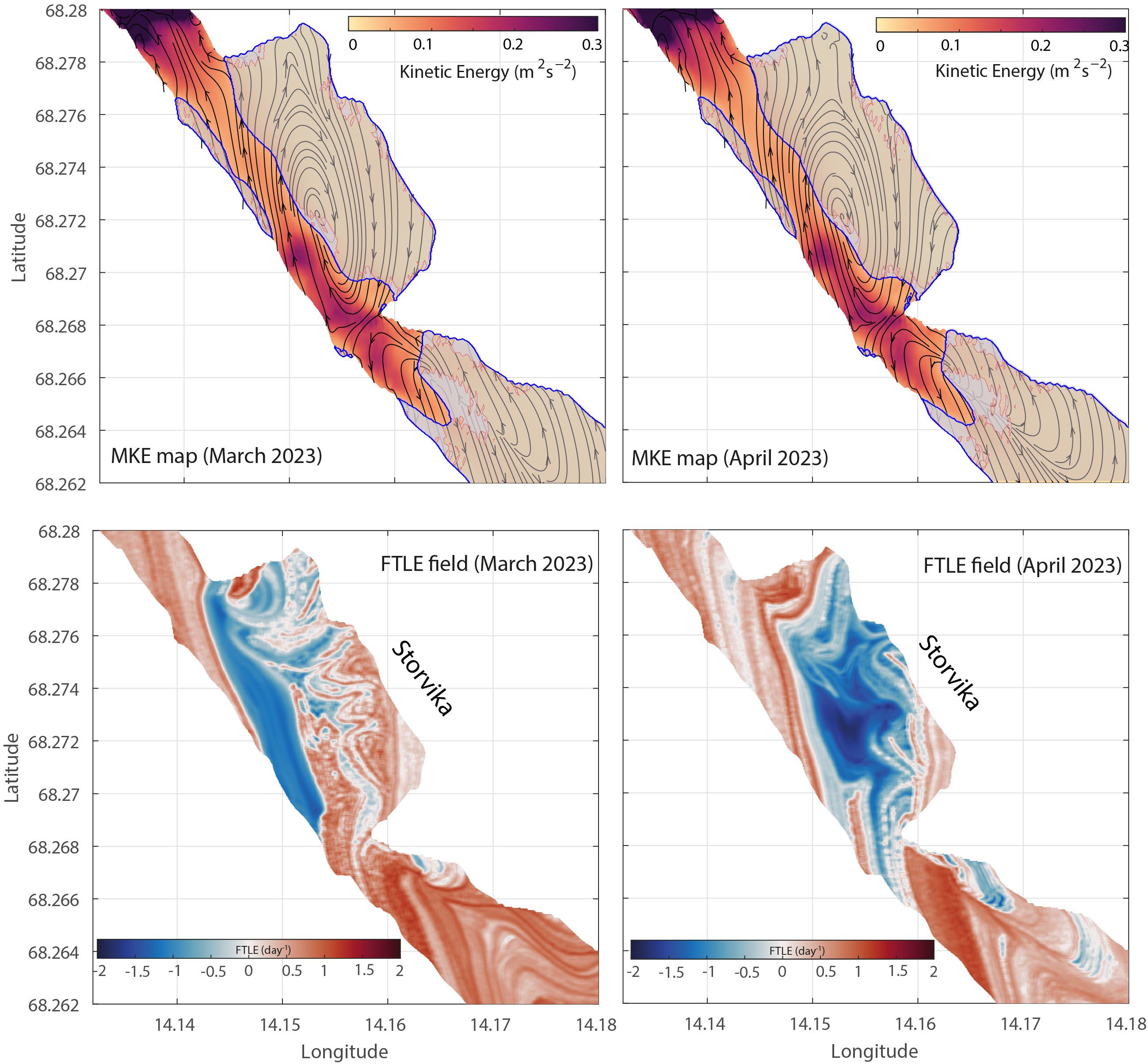
Figure 5. Spatial patterns of surface transport dynamics in the Storvika basin for March (spring tide, left) and April (neap tide, right) 2023. Top panels show MKE, (m²s⁻²) with streamlines indicating flow pathways. Blue polygons denote low-energy zones (MKE< 0.025 m² s⁻²), and red polygons highlight candidate retention zones with weak vortex circulation. Bottom panels present FTLE fields showing repelling (red) and attracting (blue) structures.

$\begin{array}{ll}U=\overline{U}+U^{\prime },& (10)\end{array}$

where U is the instantaneous velocity, $\overline{U}$ the mean velocity, and $U^{\prime }$ the deviation from this mean. The residual current reflects net transport structures shaped by tidal asymmetry, bathymetric steering, and minor wind contributions (Thomson et al., 2012; Chamorro et al., 2013; Guerra et al., 2017).

MKE which is calculated using the mean velocity component from Equation 10, peaked at approximately 0.30 m² s⁻² during spring tides and decreased to 0.24 m² s⁻² during neap conditions, with maxima along constricted and deep channel sections. Recirculation zones near the northern and eastern basin boundaries displayed substantially lower MKE values, ranging from 0.02 to 0.04 m² s⁻², nearly seven times lower than in primary flushing corridors. The energy contrast ratio between corridors and recirculation zones was 5.6 during spring and 4.9 during neap conditions, mirroring observations from the Alderney Race, where neap tides reduce kinetic energy gradients by 18 − 22% due to weaker hydraulic forcing (Thiébot et al., 2020). Furthermore, areas with MKE< 0.025 m² s⁻² (shown as blue polygons in Figure 5) expanded from 17% of the domain in spring to 28% in neap tides, indicating increased potential for debris retention.

The differences in energetics in the region between spring and neap tides provide a measure of circulation and mixing intensity, while the LCS analysis outlined in Section 2.5 quantifies how transport pathways respond to these energetic shifts. To capture short-term retention structures relevant to tidal modulation, the FTLE fields were computed using an integration window of τ = 2 day, which is a standard choice in coastal and tidal environments to resolve mesoscale flow variability and transient Lagrangian features (Serra et al., 2017; Haller, 2015; Lekien and Ross, 2010). Figure 5 presents the FTLE fields for March (spring tide) and April (neap tide) 2023. Positive FTLE values delineate repelling structures acting as dynamic barriers, while negative FTLE values highlight convergence zones where floating material accumulates. In March, repelling LCSs dominated along the main channel and boundaries, with strong transport pathways facilitating efficient export. Nevertheless, localized attracting features (FTLE values below −1.0 day⁻¹) appeared along the western boundary and lower strait, forming transient retention pockets with particle residence times of 1.5–2.2 hours, consistent with retention times reported for similar tidal environments (Leonard and Lucas, 2020).

During neap tides in April, convergence zones became more extensive, especially in the central basin and eastern boundary, with FTLE minima reaching approximately −2.0 day⁻¹. Particle residence times within these structures increased to 4 hours, and the spatial extent of strong attracting LCS regions expanded by around 40% compared to March. This corresponded with a flush-out time increase from 10 to 15 hours and a 38% increase in the Retention Efficiency Index (REI), from 0.42 to 0.58. These results indicate that weaker tidal forcing substantially enhances both the spatial and temporal scales of retention, in agreement with prior observations in barotropic archipelago systems (Børve et al., 2021). The eastern basin, particularly between latitudes 68.274°N − 68.278°N and longitudes 14.15°E − 14.16°E, exhibited moderate FTLE gradients (0.5–1.5 day⁻¹), suggesting more gradual fluid stretching and mixing. Fine-scale convergence filaments along the northeastern margin, revealed by LCS analysis but not evident in Eulerian fields or residence metrics, highlight additional retention complexity likely driven by localized recirculation patterns (Haarr et al., 2024).

Transport efficiency was computed to quantify the balance between downstream flushing and local recirculation strength, defined as:

$\begin{array}{ll}TE=\frac{{\overline{U}}_c}{{\overline{U}}_r},& (11)\end{array}$

where ${\overline{U}}_c$ is the spatially averaged velocity magnitude in primary flushing pathways and ${\overline{U}}_r$ is the average tangential velocity in retention vortices. Higher TE values, in Equation 11, indicate stronger downstream transport relative to retention. TE ranged from 2.6 during neap conditions to 4.2 under spring tides, representing a ∼ 62% increase in transport efficiency with stronger tidal forcing. This pattern confirms that energetic tidal conditions enhance flushing, while weaker tides promote retention, consistent with the findings of Gao et al. (2023) and prior studies highlighting alternating debris transport patterns controlled by tidal inequality (Schreyers et al., 2024; Sawan et al., 2025; Carvalho et al., 2025).

3.4 Residence time

While kinetic energy and streamline patterns offer qualitative insight into the distribution of energetic versus quiescent flow regions, quantifying particle retention requires a direct Lagrangian approach. To characterize spatial retention variability in Storevika, we computed residence time and revisit probability fields as outlined in Section 2.5 for March (spring tide) and April (neap tide) 2023 using particle-tracking experiments over the Storvika–Sundklakkstraumen subdomain.

Figure 6 shows the spatial distribution of mean residence time (left) and revisit probability (right). During March’s spring tide, residence times remained low basin-wide, averaging between 10 − 13.5 min. In contrast, April’s neap tides increased both the magnitude and spatial extent of residence time. The interior basin reached over 15 mins, and median values rose by nearly 40%, consistent with broader LCS convergence zones and longer flush-out times.

Figure 6

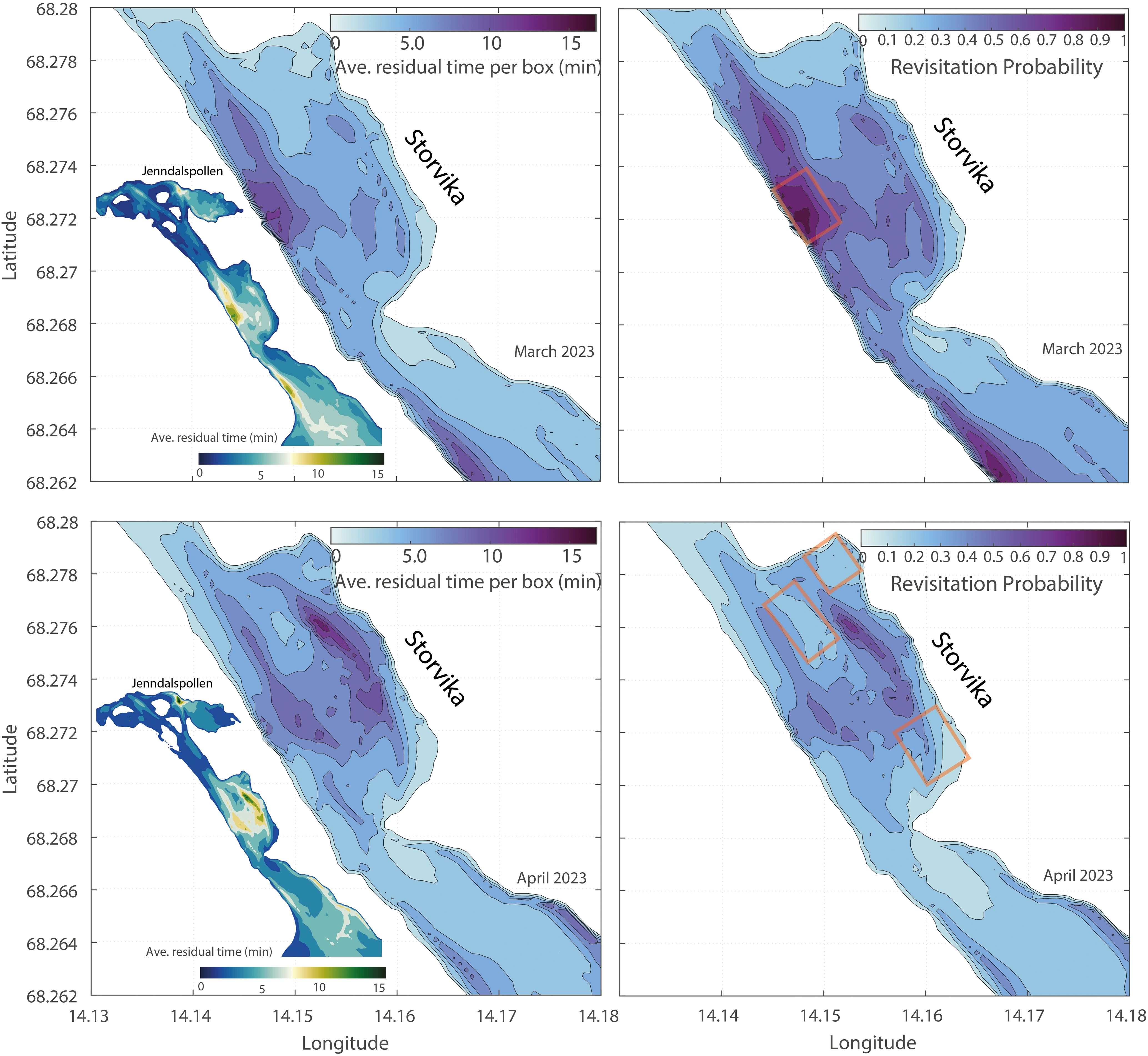
Figure 6. The maps illustrate key movement metrics for March and April 2023, including average residual time per box (left) and revisitation probability (right). Warmer colors indicate higher values, highlighting areas with prolonged retention and frequent revisits. The inset maps show normalized unique visitor probability, emphasizing spatial variation in movement patterns.

The small inset maps further resolve retention features. Highest retention was found in three distinct hotspots under neap forcing: the northeastern Storvika shoreline (near 68.276°N, 14.163^°E), the central basin (68.273°N, 14.157°E), and the sheltered entrance to Jenndalspollen (68.272°N, 14.147°E). These areas maintained residence times exceeding 15 min and revisit probabilities greater than 0.8. Ranked by relative retention intensity, the northeastern Storvika region exhibited the highest accumulation (over 18 min and revisit probability > 0.9), followed by the central basin (approximately 16.5 min and revisit ∼ 0.85), and the entrance to Jenndalspollen (around 16 min and revisit ∼ 0.82). Collectively, these zones covered about 22–25% of the domain during neap tides, in contrast to only 11–13% during spring tides. Their location correlated strongly with low-MKE pockets and attracting LCS filaments (Figure 5), suggesting coherent control by bathymetric constraints and tidally modulated forcing.

In March, revisits were concentrated near the western shoreline but remained limited in spatial coverage and persistence. The shift of recirculation and retention structures from west to east under weaker tidal amplitude reflects a redistribution of accumulation potential, in line with tidal rectification theory (Børve et al., 2021). The total particle-time spent within the domain, normalized by maximum simulation duration, increases from 0.42 to 0.58 between spring and neap tides. This increase mirrors convergence zone expansion and confirms that tidally modulated energy gradients and local topography drive systematic retention shifts in this fjordic system (Leonard and Lucas, 2020; Gao et al., 2023; Carvalho et al., 2025).

3.5 Integrated performance and hotspot metrics

To synthesize the system-scale behavior under varying tidal regimes, we combined Lagrangian diagnostics, model performance metrics, and spatial retention analysis. This integrated assessment links model accuracy with observed debris retention patterns and reveals how neap and spring tides drive contrasting accumulation dynamics within the domain.

Model skill metrics corroborate these findings. Based on normalized cumulative separation distance, the 2D and 3D models yielded overall skill scores of ss = 0.804 and ss = 0.833, respectively, placing both in the “good” performance category (Liu and Weisberg, 2011). Skill varied by tidal phase: under spring tide, the 2D and 3D models achieved ss = 0.788 and 0.802, while under neap tide, scores improved to 0.819 and 0.848. Although the improvement is modest, deployment of fewer drifters and the higher retrieval success during neap tide (an increase of up to 40%) may have contributed to better skill score estimates by increasing trajectory lengths and reducing early terminations. Endpoint displacement errors remained within 65 − 100 meters, and trajectory accuracies exceeded 87% in all cases, confirming the model’s high fidelity in representing observed pathways.

Model simulations reproduced these dynamics with high accuracy. MKE peaked near 0.30 m² s⁻² during spring tide and declined to 0.24 m² s⁻² during neap tide. Zones of low MKE (< 0.025 m² s⁻²) expanded by more than 60%, particularly near basin margins, and corresponded to convergence zones in streamline and particle tracking results. FTLE maps revealed extensive attracting LCS during neap tides, with minimum FTLE values reaching −2.0 day⁻¹ and a 40% increase in attracting area. Concurrently, median residence time increased by 40%, maximum revisit probability rose from 0.6 to 0.9, and domain-wide retention efficiency improved from 0.42 to 0.58, consistent with prior Lagrangian studies on tidal retention (Leonard and Lucas, 2020; Gao et al., 2023; Sawan et al., 2025; Carvalho et al., 2025).

These system-scale metrics are summarized in Table 2. Neap tides were associated with broader convergence zones, elevated retention, and longer particle persistence. Transport efficiency decreased from 4.2 to 2.6, and the energy contrast between flushing corridors and recirculating zones declined by 12.5%, indicating weaker energetic segregation of the basin.

Table 2

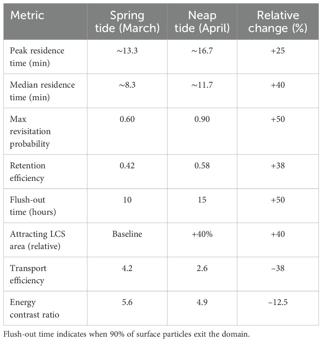
Table 2. Summary of key transport and retention metrics for spring (March) and neap (April) tide conditions in Storvika and Sundklakkstraumen.

To identify key accumulation areas, we integrated Eulerian (MKE, streamlines) and Lagrangian (residence time, revisit probability, FTLE) diagnostics with drifter trajectories. During neap tide, three hotspots were consistently observed (red zones, Figure 6). The central-northern basin (near 68.2765°N, 14.155°E) emerged as the most prominent retention zone, exhibiting > 16.5 min residence times, revisit probabilities > 0.85, and strongly attracting FTLE structures. The northeastern corner (68.2778°N, 14.1615°E) showed secondary retention, with frequent re-entrainment, while the southeastern boundary (68.2725°N, 14.161°E) exhibited intermittent stagnation. Collectively, these zones accounted for over 40% of total residence time despite covering only ∼ 20% of the basin area.

These spatial patterns are quantitatively visualized in Figure 7, which compares residence time, revisit probability, and LCS attracting area contributions across zones and tidal regimes. Under neap tide, central north Storvika contributed 25–30% to key metrics, while northeast and southeast zones contributed 8–20%. In contrast, spring tide contributions from all three zones dropped significantly, down to 10% or less, with > 74% of all metrics dominated by the rest of the basin, confirming that no persistent accumulation occurred under strong tidal forcing. Under spring tide, only one minor and transient hotspot (red zone, Figure 6) was identified along the western-central boundary of Storvika (68.2735°N, 14.146°E), where looping drifter trajectories and low-FTLE convergence coincided with slightly elevated residence times (10–11.5 min). However, this zone was small, weakly retentive, and short-lived, with retention contributions< 10% across all metrics.

Figure 7

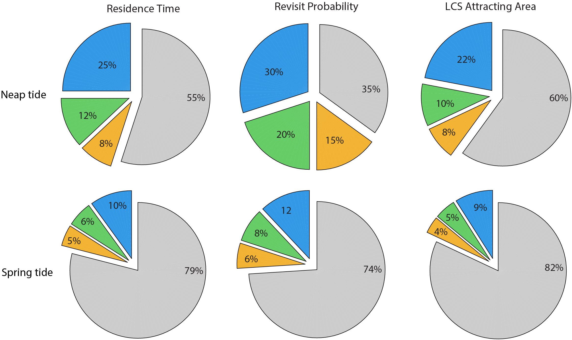
Figure 7. Retention metrics of identified hotspot locations under neap (top row) and spring (bottom row) tide conditions. Pie charts show the percentage contribution of three key diagnostics—residence time, revisit probability, and attracting LCS area—partitioned across central-north (blue), northeast (green), and southeast (orange) hotspot zones, as well as the rest of the basin (gray).

3.6 Applicability of the diagnostic approach

The multi-diagnostic approach presented here integrates observational validation, high-resolution hydrodynamic modeling, and Lagrangian diagnostics to quantify floating debris dynamics and retention under varying tidal conditions. The results align with previous reports on tidal asymmetry and plastic accumulation in high-latitude fjordic environments (Solbakken et al., 2022; Haarr et al., 2024; Børve et al., 2021), confirming that tidal modulation is a dominant control on short-term debris entrapment in complex coastal systems.

While this study focused on a sheltered fjord with minimal wind and wave influence, the same approach could be adapted to more exposed or stratified coastal systems by incorporating additional physical forcings such as wind drag, Stokes drift, and shoreline interaction schemes. For instance, Ghaffari et al. (2020) demonstrated that Stokes drift can drive transport at magnitudes comparable to moderate winds in semienclosed basins. Similarly, recent findings in the Lofoten archipelago indicate that Stokes parameterizations, particularly those accounting for crossing windsea and swell, can significantly reduce residence time near the coast (Espenes et al., 2024).

For broader application, several variables are critical, including accurate bathymetry, representative tidal forcing, and careful selection of model dimensionality (2D vs. 3D) based on the degree of baroclinicity. For the present study area, the depth-averaged 2D model proved computationally efficient and suitable for real-time operational contexts such as search and rescue (SAR), oil spill response, or aquaculture risk forecasting (Liu and Weisberg, 2011; Lebreton and Andrady, 2019). However, this substitution must be evaluated on a case-by-case basis. In fjord systems with strong stratification and significant baroclinic variability, such as Nesnafjord in northern Norway (Ghaffari et al., 2025), full 3D modeling remains essential to resolve vertical shear and associated transport processes. Additionally, in more exposed environments, the inclusion of wind and wave-induced processes becomes essential to realistically capture surface transport dynamics. Access to drifter data or equivalent observational benchmarks can further improve model calibration and transferability.

Nonetheless, certain limitations in the present setup should be noted. Wind forcing, Stokes drift, and wave effects were excluded due to the sheltered nature of the study site, which may limit direct applicability to more dynamic or open systems (Dobler et al., 2019). Reflective boundary conditions simplified shoreline interactions, potentially under-representing beaching and strandline retention processes (Hernandez et al., 2024, 2025). Likewise, while freshwater inflow was represented using climatological discharge, real-time variability, though likely minor in Lofoten, could be more consequential in river-dominated settings. Incorporating shoreline permeability and wave-driven resuspension would further improve realism in future simulations.

4 Conclusion

This study combined targeted field observations with high-resolution hydrodynamic modeling to examine the transport and retention of floating marine debris in Storvika and Sundklakkstraumen, a tidally energetic fjord system in the Lofoten archipelago. Using GPS-tracked drifters and both 2D and 3D hydrodynamic simulations, we assessed how tidal modulation governs surface transport dynamics, convergence structures, and short-term retention behavior.

Drifter deployments during spring (March 23^rd) and neap (April 14^th) tides revealed pronounced differences in surface transport. Spring tides generated strong barotropic currents that efficiently flushed particles through central channels, while neap tides favored localized recirculation and accumulation, particularly along the basin’s eastern and northern margins. Model diagnostics supported these observations, showing that neap conditions coincided with expanded retention zones, elevated residence times, and enhanced convergence as indicated by attracting Lagrangian Coherent Structures. The results confirm that tidal modulation is a dominant control on short-term debris entrapment in complex coastal systems.

The modeling results demonstrated the utility of both 2D and 3D configurations for debris transport analysis in a tidal fjord system. The 3D model resolved vertical shear and fine-scale convergence zones, whereas the depth-averaged 2D model performed well under barotropic conditions and proved computationally efficient for potential real-time applications.

In summary, this study presents a validated multi-diagnostic approach for quantifying floating debris retention in a tidally dynamic coastal system. By integrating Eulerian and Lagrangian diagnostics with empirical and simulated drifter data, the approach reveals how tidal modulation and flow structure govern the spatial and temporal dynamics of debris accumulation. Its strength lies in combining observational validation, high-resolution hydrodynamics, and multi-metric diagnostics to assess retention behavior across tidal regimes. As such, it provides a solid foundation for marine litter assessments, aquaculture planning, and operational coastal forecasting applications aimed at enhancing environmental resilience and pollution mitigation.

Data availability statement

The original contributions presented in the study are included in the article/Supplementary Material, further inquiries can be directed to the corresponding author/s.

Ethics statement

Written informed consent was obtained from the individual(s) for the publication of any identifiable images or data included in this article.

Author contributions

PG: Data curation, Project administration, Formal analysis, Conceptualization, Visualization, Validation, Methodology, Writing – original draft, Software, Writing – review & editing, Funding acquisition, Investigation, Supervision, Resources. HE: Methodology, Writing – original draft, Investigation, Data curation, Visualization, Writing – review & editing, Formal analysis. EB: Writing – review & editing. SH: Writing – review & editing. ØL: Validation, Writing – review & editing. JR: Writing – review & editing. RP: Writing – review & editing. VSS: Writing – review & editing, Funding acquisition, Project administration. MLH: Writing – review & editing, Project administration, Funding acquisition.

Funding

The author(s) declare financial support was received for the research and/or publication of this article. This work was supported by the Havplastmodellen Project (grant ID 322783) funded by The Regional Research Fund Northern Norway. The original model grid generation was supported by the GLIDER project, which was funded by the DEMO2000 research program: Norwegian Research Council and ConocoPhillips, project 269188, “Unmanned ocean vehicles, a flexible and cost-efficient offshore monitoring and data management approach”. Norwegian Research Council and ConocoPhillips were not involved in the study design, collection, analysis, interpretation of data, the writing of this article, or the decision to submit it for publication.

Acknowledgments

The authors acknowledge the Regional Research Fund Northern Norway for financial support and the Norwegian e-infrastructure for facilitating computational and data storage capacities.

Conflict of interest

Authors JR, RP, VSS, and MLH were employed by SaltLofoten.

The remaining authors declare that the research was conducted in the absence of any commercial or financial relationships that could be construed as a potential conflict of interest.

Generative AI statement

The author(s) declare that no Generative AI was used in the creation of this manuscript.

Publisher’s note

All claims expressed in this article are solely those of the authors and do not necessarily represent those of their affiliated organizations, or those of the publisher, the editors and the reviewers. Any product that may be evaluated in this article, or claim that may be made by its manufacturer, is not guaranteed or endorsed by the publisher.

Supplementary Material

The Supplementary Material for this article can be found online at: https://www.frontiersin.org/articles/10.3389/fmars.2025.1612395/full#supplementary-material

References

Adame C. M., Gacutan J., Charlesworth B., and Roughan M. (2025). Unravelling coastal plastic pollution dynamics along southeastern Australia: Insights from oceanographic modelling informed by empirical data. Mar. pollut. Bull. 213, 117525. doi: 10.1016/j.marpolbul.2024.117525

PubMed Abstract | Crossref Full Text | Google Scholar

Barron C. N., Smedstad L. F., Dastugue J. M., and Smedstad O. M. (2007). Evaluation of ocean models using observed and simulated drifter trajectories: Impact of sea surface height on synthetic profiles for data assimilation. J. Geophysical Rese: Oceans 112 (C7), C07019. doi: 10.1029/2006JC003982

Crossref Full Text | Google Scholar

Beldring S., Engeland K., Roald L. A., Sælthun N. R., and Voksø A. (2003). Estimation of parameters in a distributed precipitation-runoff model for Norway. Hydrol. Earth Syst. Sci. 7, 304–316. doi: 10.5194/hess-7-304-2003

Crossref Full Text | Google Scholar

Bellou N., Gambardella C., Karantzalos K., Monteiro J. G., Canning-Clode J., Kemna S., et al. (2021). Global assessment of innovative solutions to tackle marine litter. Nat. Sustainability 4, 516–524. doi: 10.1038/s41893-021-00726-2

Crossref Full Text | Google Scholar

Benjamins S., Dale A. C., Hastie G., Waggitt J. J., Lea M.-A., Scott B., et al. (2015). Confusion reigns? a review of marine megafauna interactions with tidal-stream environments. Oceanography Mar. Biol.: Annu. Rev. 53, 1–54.

Google Scholar

Beron-Vera F. J., Wang Y., Olascoaga M. J., Goni G. J., and Haller G. (2013). Objective detection of oceanic eddies and the agulhas leakage. J. Phys. Oceanography 43, 1426–1438. doi: 10.1175/JPO-D-12-0171.1

Crossref Full Text | Google Scholar

Bianucci L., Jackson J. M., Allen S. E., Krassovski M. V., Giesbrecht I. J., and Callendar W. C. (2024). Fjord circulation permits a persistent subsurface water mass in a long, deep mid-latitude inlet. Ocean Sci. 20, 293–306. doi: 10.5194/os-20-293-2024

Crossref Full Text | Google Scholar

Børve E., Isachsen P. E., and Nøst O. A. (2021). Rectified tidal transport in lofoten–vesterålen, northern Norway. Ocean Sci. 17, 1753–1773.

Google Scholar

Børve E., Isachsen P. E., Nøst O. A., Ghaffari P., and Falk-Petersen S. (2025). Tidal effects on transport and dispersion of particles, cod eggs and larvae in the lofoten and vesterålen region, Norway. Front. Mar. Sci. 12. doi: 10.3389/fmars.2025.1541652

Crossref Full Text | Google Scholar

Browne M. A., Crump P., Niven S. J., Teuten E., Tonkin A., Galloway T., et al. (2011). Accumulation of microplastic on shorelines woldwide: sources and sinks. Environ. Sci. Technol. 45, 9175–9179. doi: 10.1021/es201811s

PubMed Abstract | Crossref Full Text | Google Scholar

Callies U., Groll N., Horstmann J., Kapitza H., Klein H., Maßmann S., et al. (2017). Surface drifters in the german bight: model validation considering windage and stokes drift. Ocean Sci. 13, 799–827. doi: 10.5194/os-13-799-2017

Crossref Full Text | Google Scholar

Carvalho D. G. D., Gaylarde C. C., Lourenco M. F. d. P., MaChado W. T. V., and Baptista Neto J. A. (2025). Seasonal variations in microplastic pollution in beach sediments along the eastern coast of rio de janeiro state, Brazil. J. Coast. Res. 41, 291–304. doi: 10.2112/JCOASTRES-D-24-00025.1

Crossref Full Text | Google Scholar

Chamorro L., Hill C., Morton S., Ellis C., Arndt R., and Sotiropoulos F. (2013). On the interaction between a turbulent open channel flow and an axial-flow turbine. J. Fluid Mechanics 716, 658–670. doi: 10.1017/jfm.2012.571

Crossref Full Text | Google Scholar

Chen C., Beardsley R. C., Cowles G., Qi J., Lai Z., Gao G., et al. (2006). An unstructured grid, finite-volume coastal ocean model: Fvcom user manual. SMAST/UMASSD. Cambridge, MA: MIT Sea Grant College Program. p. 6–8. Available online at: http://fvcom.smast.umassd.edu/wp-content/uploads/2013/11/MITSG_12-25.pdf.

Google Scholar

Chen C., Liu H., and Beardsley R. C. (2003). An unstructured grid, finite-volume, three-dimensional, primitive equations ocean model: application to coastal ocean and estuaries. J. Atmospheric Oceanic Technol. 20, 159–186. doi: 10.1175/1520-0426(2003)020<0159:AUGFVT>2.0.CO;2

Crossref Full Text | Google Scholar

Coulliette C. and Wiggins S. (2001). Intergyre transport in a wind-driven, quasigeostrophic double gyre: An application of lobe dynamics. Nonlinear Processes Geophysics 8, 69–94. doi: 10.5194/npg-8-69-2001

Crossref Full Text | Google Scholar

Cowton T., Slater D., Sole A., Goldberg D., and Nienow P. (2015). Modeling the impact of glacial runoff on fjord circulation and submarine melt rate using a new subgrid-scale parameterization for glacial plumes. J. Geophysical Rese: Oceans 120, 796–812. doi: 10.1002/2014JC010324

Crossref Full Text | Google Scholar

Cózar A., Echevarría F., González-Gordillo J. I., Irigoien X., Úbeda B., Hernández-León S., et al. (2014). Plastic debris in the open ocean. Proc. Natl. Acad. Sci. 111, 10239–10244. doi: 10.1073/pnas.1314705111

PubMed Abstract | Crossref Full Text | Google Scholar

Dagestad K.-F., Breivik Ø., and Ådlandsvik B. (2016). “Opendrift-an open source framework for ocean trajectory modeling,” in EGU General Assembly Conference Abstracts. EPSC2016–7282. Vienna, Austria:European Geosciences Union, 18, Egu2016-7282. Available online at: https://ui.adsabs.harvard.edu/abs/2016EGUGA..18.7282D/abstract.

Google Scholar

Dagestad K.-F., Röhrs J., Breivik Ø., and Ådlandsvik B. (2018). Opendrift v1. 0: a generic framework for trajectory modelling. Geosci. Model. Dev. 11, 1405–1420. doi: 10.5194/gmd-11-1405-2018

Crossref Full Text | Google Scholar

Dalsøren S. B., Albretsen J., and Asplin L. (2020). New validation method for hydrodynamic fjord models applied in the Hardangerfjord, Norway. Estuarine Coast. Shelf Sci. 246, 107028. doi: 10.1016/j.ecss.2020.107028

Crossref Full Text | Google Scholar

Davis R. E. (1985). Drifter observations of coastal surface currents during code: The method and descriptive view. J. Geophysical Rese: Oceans 90, 4741–4755. doi: 10.1029/JC090iC03p04741

Crossref Full Text | Google Scholar

de Swart H. E. and Yuan B. (2019). Dynamics of offshore tidal sand ridges, a review. Environ. Fluid Mechanics 19, 1047–1071. doi: 10.1007/s10652-018-9630-8

Crossref Full Text | Google Scholar

Dobler D., Huck T., Maes C., Grima N., Blanke B., Martinez E., et al. (2019). Large impact of stokes drift on the fate of surface floating debris in the south Indian basin. Mar. pollut. Bull. 148, 202–209. doi: 10.1016/j.marpolbul.2019.07.057

PubMed Abstract | Crossref Full Text | Google Scholar

Elipot S. and Beal L. M. (2015). Characteristics, energetics, and origins of agulhas current meanders and their limited influence on ring shedding. J. Phys. Oceanography 45, 2294–2314. doi: 10.1175/JPO-D-14-0254.1

Crossref Full Text | Google Scholar

Espenes H., Carrasco A., Dagestad K.-F., Christensen K. H., Drivdal M., and Isachsen P. E. (2024). Stokes drift in crossing windsea and swell, and its effect on near-shore particle transport in lofoten, northern Norway. Ocean Model. 191, 102407. doi: 10.1016/j.ocemod.2024.102407

Crossref Full Text | Google Scholar

Espenes H., Isachsen P. E., and Nøst O. A. (2023). Observations and modelling of tidally generated high-frequency velocity fluctuations downstream of a channel constriction. EGUsphere 2023, 1–24. doi: 10.5194/egusphere-2023-214

Crossref Full Text | Google Scholar

Fox-Kemper B., Danabasoglu G., Ferrari R., Griffies S., Hallberg R., Holland M., et al. (2011). Parameterization of mixed layer eddies. iii: Implementation and impact in global ocean climate simulations. Ocean Model. 39, 61–78. doi: 10.1016/j.ocemod.2010.09.002

Crossref Full Text | Google Scholar

Gao G., O’Sullivan J. J., Corkery A., Bedri Z., O’Hare G. M., and Meijer W. G. (2023). The use of transport time scales as indicators of pollution persistence in a macro-tidal setting. J. Mar. Sci. Eng. 11 (5), 1073. doi: 10.3390/jmse11051073

Crossref Full Text | Google Scholar

Ghaffari P., Isachsen P., and LaCasce J. (2013). Topographic effects on current variability in the caspian sea. J. Geophysical Rese: Oceans 118, 7107–7116. doi: 10.1002/2013JC009128

Crossref Full Text | Google Scholar

Ghaffari P., Isachsen P. E., Nøst O. A., and Weber J. E. (2018). The influence of topography on the stability of the norwegian atlantic current off northern Norway. J. Phys. Oceanography 48, 2761–2777. doi: 10.1175/JPO-D-17-0235.1

Crossref Full Text | Google Scholar

Ghaffari P., Jonassen T. M., Kvam J., and Staven F. (2025). Behavioral response of farmed cod to environmental drivers and interaction with feeding practice. Aquacult. Eng. 111, 102560. doi: 10.1016/j.aquaeng.2025.102560

Crossref Full Text | Google Scholar

Ghaffari P., Sperrevik A.-K., Nøst O. A., Christensen K. H., and Camus L. (2019). “Complementary role of glider data on the modeling of multi-scale dynamics in the norwegian coastal and fjord regions,” in OCEANS 2019-Marseille (Piscataway, NJ, USA: IEEE), 1–6. doi: 10.1109/OCEANSE.2019.8867127

Crossref Full Text | Google Scholar

Ghaffari P., Weber J. E. H., Nøst O. A., and Drivdal M. (2020). Stokes drift in topographic waves over an enclosed basin shelf. J. Phys. Oceanography 50, 1197–1211. doi: 10.1175/JPO-D-19-0126.1

Crossref Full Text | Google Scholar

Guerra M., Cienfuegos R., Thomson J., and Suarez L. (2017). Tidal energy resource characterization in chacao channel, Chile. Int. J. Mar. Energy 20, 1–16. doi: 10.1016/j.ijome.2017.11.002

Crossref Full Text | Google Scholar

Haarr M. L., Rydsaa J., Pires R., Espenes H., Hermansen S., Ghaffari P., et al. (2024). Beach litter deposition and turnover, effects of tides and weather, and implications for cleanup strategies: A case study in the lofoten archipelago, Norway. Mar. pollut. Bull. 206, 116720. doi: 10.1016/j.marpolbul.2024.116720

PubMed Abstract | Crossref Full Text | Google Scholar

Haller G. (2015). Lagrangian coherent structures. Annu. Rev. Fluid Mechanics 47, 137–162. doi: 10.1146/annurev-fluid-010313-141322

Crossref Full Text | Google Scholar

Hecht M. W. and Hasumi H. (2013). Ocean modeling in an eddying regime (Washington, DC, USA: John Wiley & Sons) 177, 409. Available online at: https://books.google.com/books?id=4isBdNVuQbgC.

Google Scholar

Hernandez I., Castro-Rosero L. M., Espino M., and Alsina J. M. (2025). Processes controlling the dispersion and beaching of floating marine debris in the barcelona coastal region. Front. Mar. Sci. 11, 1534678. doi: 10.3389/fmars.2024.1534678

Crossref Full Text | Google Scholar

Hernandez I., Castro-Rosero L. M., Espino M., and Alsina Torrent J. M. (2024). Locate v1. 0: numerical modelling of floating marine debris dispersion in coastal regions using parcels v2. 4.2. Geosci. Model. Dev. 17, 2221–2245. doi: 10.5194/gmd-17-2221-2024

Crossref Full Text | Google Scholar

Hunter E. J., Fuchs H. L., Wilkin J. L., Gerbi G. P., Chant R. J., and Garwood J. C. (2022). Romspath v1. 0: offline particle tracking for the regional ocean modeling system (roms). Geosci. Model. Dev. 15, 4297–4311. doi: 10.5194/gmd-15-4297-2022

Crossref Full Text | Google Scholar

Jalón-Rojas I., Sous D., and Marieu V. (2024). A wave-resolving 2dv lagrangian approach to model microplastic transport in the nearshore. Geosci. Model. Dev. Discussions 2024, 1–26. doi: 10.5194/gmd-2024-100

Crossref Full Text | Google Scholar

Jing T., Chen R., Liu C., Qiu C., Zhang C., and Hong M. (2025). Global surface eddy mixing ellipses: spatio-temporal variability and machine learning prediction. Front. Mar. Sci. 11, 1506419. doi: 10.3389/fmars.2024.1506419

Crossref Full Text | Google Scholar

Kobayashi M. H., Pereira J. M., and Pereira J. C. (1999). A conservative finite-volume second-order-accurate projection method on hybrid unstructured grids. J. Comput. Phys. 150, 40–75. doi: 10.1006/jcph.1998.6163

Crossref Full Text | Google Scholar

Kontogiannis G. and Bakas N. A. (2020). A geometric interpretation of zonostrophic instability. J. Phys. Oceanography 50, 2759–2779. doi: 10.1175/JPO-D-19-0255.1

Crossref Full Text | Google Scholar

Kristensen N. M. and Gusdal Y. (2021). Norkyst800 model currents validation. MET Report,(2/2021) Vol. 44 (Oslo, Norway: Norwegian Meteorological Institute). Available online at: https://www.met.no/publikasjoner/met-report/met-report-2021/_/attachment/download/8b99ea1b-200f-4a09-9eb7-3ada0580e157:56ff9d6c44186aa495be038a1cc5dd84d3ca3f2a/MET-report-02-2021.pdf.

Google Scholar

Kurogi M. and Hasumi H. (2019). Tidal control of the flow through long, narrow straits: a modeling study for the seto inland sea. Sci. Rep. 9, 11077. doi: 10.1038/s41598-019-47090-y

PubMed Abstract | Crossref Full Text | Google Scholar

Lebreton L. and Andrady A. (2019). Future scenarios of global plastic waste generation and disposal. Palgrave Commun. 5, 1–11. doi: 10.1057/s41599-018-0212-7

Crossref Full Text | Google Scholar

Lekien F. and Ross S. D. (2010). The computation of finite-time lyapunov exponents on unstructured meshes and for non-euclidean manifolds. Chaos: Interdiscip. J. Nonlinear Sci. 20, 017505. doi: 10.1063/1.3278516

PubMed Abstract | Crossref Full Text | Google Scholar

Leonard E. and Lucas M. (2020). Identifying plastic accumulation zones in coastal seas: The roatan island case study. Mar. pollut. Bull. 154, 111077. doi: 10.1016/j.marpolbul.2020.111077

PubMed Abstract | Crossref Full Text | Google Scholar

Le Traon P. and Morrow R. (2001). “Ocean currents and eddies,” in International Geophysics, vol. 69. (San Diego, CA, USA: Elsevier), 171–1xi. doi: 10.1016/S0074-6142(01)80148-0

Crossref Full Text | Google Scholar

Liu Y. and Weisberg R. H. (2011). Evaluation of trajectory modeling in different dynamic regions using normalized cumulative lagrangian separation. J. Geophysical Rese: Oceans 116, 1–17. doi: 10.1029/2010JC006837

Crossref Full Text | Google Scholar

Lumpkin R. and Johnson G. C. (2013). Global ocean surface velocities from drifters: Mean, variance, el niño–southern oscillation response, and seasonal cycle. J. Geophysical Rese: Oceans 118, 2992–3006. doi: 10.1002/jgrc.20210

Crossref Full Text | Google Scholar

Lynge B. K., Berntsen J., and Gjevik B. (2010). Numerical studies of dispersion due to tidal flow through moskstraumen, northern Norway. Ocean Dynamics 60, 907–920. doi: 10.1007/s10236-010-0309-z

Crossref Full Text | Google Scholar

McWilliams J. C. (2016). Submesoscale currents in the ocean. Proc. R. Soc. A.: Mathematical Phys. Eng. Sci. 472, 20160117. doi: 10.1098/rspa.2016.0117

PubMed Abstract | Crossref Full Text | Google Scholar

Mitchelson-Jacob G. and Sundby S. (2001). Eddies of Vestfjorden, Norway. Continental Shelf Res. 21, 1901–1918. doi: 10.1016/S0278-4343(01)00030-9

Crossref Full Text | Google Scholar

Moe H., Ommundsen A., and Gjevik B. (2002). A high resolution tidal model for the area around the Lofoten Islands, Northern Norway. Continental Shelf Res. 22, 485–504. doi: 10.1016/S0278-4343(01)00078-4

Crossref Full Text | Google Scholar

Müller M., Homleid M., Ivarsson K.-I., Køltzow M. A., Lindskog M., Midtbø K. H., et al. (2017). Arome-metcoop: A nordic convective-scale operational weather prediction model. Weather Forecasting 32, 609–627. doi: 10.1175/WAF-D-16-0099.1

Crossref Full Text | Google Scholar

Nøst O. A. and Børve E. (2021). Flow separation, dipole formation and water exchange through tidal strait. Ocean Sci. Discussions 2021, 1–34. doi:  10.5194/os-17-1403-2021

Crossref Full Text | Google Scholar

Onink V., Jongedijk C. E., Hoffman M. J., van Sebille E., and Laufkötter C. (2021). Global simulations of marine plastic transport show plastic trapping in coastal zones. Environ. Res. Lett. 16, 064053. doi: 10.1088/1748-9326/abecbd

Crossref Full Text | Google Scholar

Opdal A. F., Vikebø F. B., and Fiksen Ø. (2008). Relationships between spawning ground identity, latitude and early life thermal exposure in northeast arctic cod. 41, 13–22. doi: 10.2960/J.v41.m621

Crossref Full Text | Google Scholar

Özgökmen T. M., Griffa A., Mariano A. J., and Piterbarg L. I. (2000). On the predictability of lagrangian trajectories in the ocean. J. Atmospheric Oceanic Technol. 17, 366–383. doi: 10.1175/1520-0426(2000)017<0366:OTPOLT>2.0.CO;2

Crossref Full Text | Google Scholar

Pawlowicz R. (2021). The grounding of floating objects in a marginal sea. J. Phys. Oceanography 51, 537–551. doi: 10.1175/JPO-D-20-0183.1

Crossref Full Text | Google Scholar

Peacock T. and Haller G. (2013). Lagrangian coherent structures: The hidden skeleton of fluid flows. Phys. Today 66, 41–47. doi: 10.1063/PT.3.1886

Crossref Full Text | Google Scholar

Pieterse A., Puleo J. A., McKenna T. E., and Aiken R. A. (2015). Near-bed shear stress, turbulence production and dissipation in a shallow and narrow tidal channel. Earth Surface Processes Landforms 40, 2059–2070. doi: 10.1002/esp.v40.15

Crossref Full Text | Google Scholar

Röhrs J., Sperrevik A. K., and Christensen K. H. (2018). Norshelf: A reanalysis and data-assimilative forecast model for the Norwegian shelf sea (Oslo, Norway: Norwegian Meteorological Institute). Available online at: https://zenodo.org/record/2384124.

Google Scholar

Saint-Amand A., Lambrechts J., Thomas C. J., and Hanert E. (2023). How fine is fine enough? Effect of mesh resolution on hydrodynamic simulations in coral reef environments. Ocean Modelling. 186, 102254. doi: 10.31223/X5DM1Q

Crossref Full Text | Google Scholar

Sawan R., Doyen P., Veillet G., Viudes F., Mahfouz C., and Amara R. (2025). Mobilization and deposition of plastic along an estuarine bank during tidal cycles. Heliyon. 11 (2), e42026. doi: 10.1016/j.heliyon.2025.e42026

PubMed Abstract | Crossref Full Text | Google Scholar

Schreyers L. J., Van Emmerik T. H., Bui T.-K. L., van Thi K. L., Vermeulen B., Nguyen H.-Q., et al. (2024). River plastic transport affected by tidal dynamics. Hydrol. Earth Syst. Sci. 28, 589–610. doi: 10.5194/hess-28-589-2024

Crossref Full Text | Google Scholar

Serra M., Sathe P., Beron-Vera F., and Haller G. (2017). Uncovering the edge of the polar vortex. J. Atmospheric Sci. 74, 3871–3885. doi: 10.1175/JAS-D-17-0052.1

Crossref Full Text | Google Scholar

Shadden S. C., Lekien F., and Marsden J. E. (2005). Definition and properties of lagrangian coherent structures from finite-time lyapunov exponents in two-dimensional aperiodic flows. Physica D.: Nonlinear Phenomena 212, 271–304. doi: 10.1016/j.physd.2005.10.007

Crossref Full Text | Google Scholar

Smagorinsky J. (1963). General circulation experiments with the primitive equations: I. the basic experiment. Monthly Weather Rev. 91, 99–164. doi: 10.1175/1520-0493(1963)091<0099:GCEWTP>2.3.CO;2

Crossref Full Text | Google Scholar

Solbakken V., Kleiven S., and Haarr M. (2022). Deposition rates and residence time of litter varies among beaches in the lofoten archipelago, Norway. Mar. pollut. Bull. 177, 113533. doi: 10.1016/j.marpolbul.2022.113533

PubMed Abstract | Crossref Full Text | Google Scholar

Thiébot J., Coles D., Bennis A.-C., Guillou N., Neill S., Guillou S., et al. (2020). Numerical modelling of hydrodynamics and tidal energy extraction in the alderney race: A review. Philos. Trans. R. Soc. A. 378, 20190498. doi: 10.1098/rsta.2019.0498

PubMed Abstract | Crossref Full Text | Google Scholar

Thiringer T., MacEnri J., and Reed M. (2011). Flicker evaluation of the seagen tidal power plant. IEEE Trans. Sustain. Energy 2, 414–422. doi: 10.1109/TSTE.2011.2157182

Crossref Full Text | Google Scholar

Thompson R. C., Moore C. J., Vom Saal F. S., and Swan S. H. (2009). Plastics, the environment and human health: current consensus and future trends. Philos. Trans. R. Soc. B.: Biol. Sci. 364, 2153–2166. doi: 10.1098/rstb.2009.0053

PubMed Abstract | Crossref Full Text | Google Scholar

Thomson J., Polagye B., Durgesh V., and Richmond M. C. (2012). Measurements of turbulence at two tidal energy sites in puget sound, wa. IEEE J. Oceanic Eng. 37, 363–374. doi: 10.1109/JOE.2012.2191656

Crossref Full Text | Google Scholar

Van Sebille E., Aliani S., Law K. L., Maximenko N., Alsina J. M., Bagaev A., et al. (2020). The physical oceanography of the transport of floating marine debris. Environ. Res. Lett. 15, 023003. doi: 10.1088/1748-9326/ab6d7d

Crossref Full Text | Google Scholar

Van Sebille E., England M. H., and Froyland G. (2012). Origin, dynamics and evolution of ocean garbage patches from observed surface drifters. Environ. Res. Lett. 7, 044040. doi: 10.1088/1748-9326/7/4/044040

Crossref Full Text | Google Scholar

Van Sebille E., Griffies S. M., Abernathey R., Adams T. P., Berloff P., Biastoch A., et al. (2018). Lagrangian ocean analysis: Fundamentals and practices. Ocean Model. 121, 49–75. doi: 10.1016/j.ocemod.2017.11.008

Crossref Full Text | Google Scholar

Van Sebille E., Wilcox C., Lebreton L., Maximenko N., Hardesty B. D., Van Franeker J. A., et al. (2015). A global inventory of small floating plastic debris. Environ. Res. Lett. 10, 124006. doi: 10.1088/1748-9326/10/12/124006

Crossref Full Text | Google Scholar

Vikebø F., Jørgensen C., Kristiansen T., and Fiksen Ø. (2007). Drift, growth, and survival of larval northeast arctic cod with simple rules of behaviour. Mar. Ecol. Prog. Ser. 347, 207–219. doi: 10.3354/meps06979

Crossref Full Text | Google Scholar

Ward S., Robins P., Owen A., Demmer J., and Jenkins S. (2023). The importance of resolving nearshore currents in coastal dispersal models. Ocean Model. 183, 102181. doi: 10.1016/j.ocemod.2023.102181

Crossref Full Text | Google Scholar

Willmott C. J. (1981). On the validation of models. Phys. Geogr. 2, 184–194. doi: 10.1080/02723646.1981.10642213

Crossref Full Text | Google Scholar

Xie D., Pan C., and Wu X. (2022). “Modeling the tidal bore on the qiantang river, China: An application of fvcom,” in Environmental Hydraulics, vol. 1. (London, UK: Taylor & Francis), 331–336. doi: 10.1201/9780429100307-52

Crossref Full Text | Google Scholar

Zhang H. (2017). Transport of microplastics in coastal seas. Estuarine Coast. Shelf Sci. 199, 74–86. doi: 10.1016/j.ecss.2017.09.032

Crossref Full Text | Google Scholar

Zimmerman J. (1980). Vorticity transfer by tidal currents over an irregular topography. J. Mar. Res. 38 (4), 601--630. doi: 10.1357/002224080787537735

Crossref Full Text | Google Scholar