 Tobias Ziolkowski
 Colin W. Devey
 Agnes Koschmider2
- 1GEOMAR - Helmholtz Centrum for Ocean Research Kiel, Kiel, Germany
- 2Process Analytics Group, University of Bayreuth, Bayreuth, Germany
Seamounts play a crucial role in marine ecosystems, ocean circulation, and plate tectonics, yet most remain unmapped due to limitations in detection methods. While satellite altimetry provides large-scale coverage, its resolution is insufficient for detecting smaller seamounts, necessitating high-resolution multibeam bathymetry. This study introduces a deep-learning-based framework for automated small seamount detection in multibeam bathymetry, combining a CNN-based filtering step with U-Net segmentation to enhance accuracy and efficiency. Using multibeam bathymetric data from the SO305–2 expedition, the proposed approach successfully identified 30 seamounts, many of which were undetectable using satellite altimetry. A hyperparameter optimization study determined the optimal U-Net configuration, achieving a Dice Coefficient of 0.8274 and a Mean IoU of 0.7514. While the model performed well within the training dataset, cross-regional generalization remains challenging, with reduced accuracy observed in areas of highly variable seafloor morphology. The results highlight the limitations of satellite altimetry, as only 14 of the 30 detected seamounts were visible in satellite-derived datasets. This underscores the necessity of high-resolution multibeam surveys for capturing fine-scale seafloor features. In contrast to time-intensive manual annotation—which can require several hours to accurately delineate each individual seamount—the automated U-Net-based segmentation approach analyzed 146,060 km² of multibeam data within seconds, offering substantial time savings and scalability for large-scale mapping efforts. Beyond geological mapping, automated seamount detection has broad applications in marine ecology, environmental monitoring, and plate tectonics research. Future work should focus on integrating physical principles and geological constraints, such as typical seamount morphology, size distributions, and tectonic setting, to improve classification accuracy.
1 Introduction
Seamounts, underwater mountains formed by volcanic activity, are significant features of the ocean floor, providing important information about plate tectonics and influencing, for example, marine ecosystems, ocean circulation and global geochemical cycles. Mapping these structures is essential for advancing oceanographic and geological research. However, most seamounts remain unmapped due to limitations in detection methods.
Satellite altimetry has been widely used to detect large seamounts through gravity anomalies, but its resolution constraints hinder the identification of smaller structures. Kim and Wessel (2011) detected seamounts taller than 1,500 meters, estimating between 25,000 and 140,000 seamounts exceeding 1,000 meters in height while suggesting that up to 25 million seamounts above 100 meters remain uncharted. More recently, Gevorgian et al. (2023) expanded the global seamount catalog by identifying 19,325 new seamounts, increasing the total to 43,454. Despite these advances, the reliability of satellite altimetry in detecting small seamounts remains uncertain, particularly given the influence of data resolution and noise.
Multibeam bathymetry enables direct, high-resolution mapping of the seafloor, offering far greater detail than satellite-based methods. However, while the surveys themselves remain time-intensive and spatially constrained, the subsequent analysis and annotation of collected data present an additional bottleneck. To address this challenge, this study introduces an automated deep-learning-based framework to accelerate the detection and classification of small seamounts in multibeam datasets. The approach combines convolutional neural networks (CNNs) for initial filtering with a U-Net-based segmentation model to delineate potential seamount regions. By replacing manual annotation with a scalable two-step pipeline, the method significantly reduces the time and effort required for post-survey analysis—especially for identifying small seamounts often missed in global databases.
An additional challenge lies in understanding the morphological properties of small seamounts. Smith (1988) proposed a height-to-base radius ratio of 0.21, but it remains unclear whether this relationship holds for smaller seamounts or if geometric variations require adjustments in altimetry-based models. Addressing this question is critical for improving detection methodologies.
To systematically evaluate this approach, the study addresses the following research questions:
1. How does a filtering-based approach improve the identification of small seamounts in multibeam bathymetric data compared to manual identification?
2. What are the optimal hyperparameters for training a U-Net model to achieve the highest segmentation accuracy for small seamount detection?
3. How well does the proposed framework generalize across different geographic regions, and what limitations arise when applying a model trained in one ocean basin to another?
4. What is the effective lower detection limit of satellite altimetry for small seamounts, and how does this compare to detections from high-resolution multibeam bathymetric data?
Beyond geological mapping, automated seamount detection has broad applications in marine science. In submarine topography studies, this methodology can be extended to detect and classify other undersea features, such as ridges, trenches, and hydrothermal vent fields (Huang et al., 2024). In marine ecology, seamounts serve as biodiversity hotspots, providing habitat for deep-sea organisms; automating their detection can support conservation efforts (Clark et al., 2010). Additionally, accurate seamount mapping contributes to research on seafloor geodynamics, volcanic activity, and plate tectonics (Matabos et al., 2022). Automated bathymetric analysis also plays a critical role in environmental monitoring and deep-sea mining, assisting in landslide risk assessment and resource extraction planning (Jones et al., 2021; Usui and S, 2022).
2 Literature review
Seamount classification has been a focal point in marine geosciences, employing a range of methods from satellite altimetry to high-resolution multibeam bathymetry. Early studies, such as Smith (1988) and Mitchell (2001), primarily relied on satellite-derived gravity data to detect and classify seamounts. While effective for large-scale features, these approaches are inherently constrained by resolution limitations, as only larger seamounts generate sufficiently strong gravitational anomalies to be visible in global datasets. Multibeam bathymetry provides a higher-resolution alternative, enabling the detection of smaller features. However, its limited spatial coverage and the manual effort required for classification restrict its scalability for global mapping.
To address these challenges, machine learning techniques have been explored for automated feature extraction in bathymetric datasets. Cracknell and Reading (2014) compared various supervised learning algorithms for lithology classification, identifying Random Forests as a robust choice due to its spatial accuracy, while SVMs and k-NN exhibited computational inefficiencies and sensitivity to noise. Despite their success in broad geological classification, these methods rely on hand-engineered features, making them unsuitable for detecting complex, small-scale seamounts.
Recent advances in deep learning have significantly improved seafloor classification by automatically extracting hierarchical features from raw data. Valentine and Kalnins (2013) introduced an autoencoder-based framework to detect seamount-like features based on reconstruction errors, reducing human bias but requiring extensive training data. Similarly, Liu et al. (2024) employed YOLO V7 Tiny for detecting deepsea features under challenging imaging conditions, achieving high accuracy but struggling to generalize across diverse bathymetric terrains.
Several CNN architectures have been widely explored in geospatial and seafloor classification applications, including VGG16 (Simonyan and Zisserman, 2015), ResNet50 (He et al., 2016), InceptionV3 (Szegedy et al., 2016), and MobileNetV2 (Sandler et al., 2018). These models offer varying trade-offs in feature representation, computational efficiency, and robustness:
● VGG16 is a deep yet simple architecture, utilizing small convolutional filters to extract structured features, making it effective for hierarchical representation. However, its high computational demand limits its efficiency for large-scale datasets.
● ResNet50 introduces residual connections, allowing deeper networks while mitigating vanishing gradient issues, making it well-suited for complex pattern recognition in bathymetric data.
● InceptionV3 employs multi-scale convolutions, enhancing adaptability to seamounts of varying size and morphology.
● MobileNetV2, optimized for computational efficiency, uses depthwise separable convolutions but lacks the necessary depth and architectural components for detailed segmentation.
Given the need for efficient large-scale filtering in seamount detection, we conduct a comparative analysis of these models in Section 4.1 to evaluate their effectiveness in generating feature vectors for clustering and classification.
For detailed bathymetric segmentation, U-Net (Ronneberger et al., 2015) was selected as the core architecture due to its proven ability to combine high segmentation accuracy with computational feasibility. Originally developed for biomedical imaging, U-Net’s encoder-decoder design, augmented with skip connections, ensures that both contextual and spatial information is preserved—critical for detecting small, irregularly shaped seamounts in multibeam bathymetric data. Unlike classification models that provide a single output per image or object detectors that require bounding boxes, U-Net performs dense pixel-wise labeling, which is particularly suited for the continuous and ambiguous topography of the seafloor. Its relatively low data requirements and efficient training regime further make it a practical solution for seafloor mapping tasks where labeled data is limited.
Other segmentation architectures, though effective in image processing, exhibit notable limitations:
● DeepLabV3+: Chen et al. (2018), while capturing multi-scale context through atrous convolutions, is computationally expensive.
● Mask R-CNN: He et al. (2017) excels in instance segmentation but relies on predefined object boundaries, making it less suitable for the continuous, often ambiguous topographies of seamounts.
● YOLO-based models: Wang and Bochkovskiy (2022), while optimized for real-time object detection, lack the granularity required for detailed segmentation.
Given these considerations, U-Net provides the best balance between segmentation accuracy and computational efficiency. Its architecture is uniquely suited for small seamount segmentation, enabling robust detection even under conditions of sparse training data and morphologically complex targets.
The increasing availability of high-resolution bathymetric datasets has led to a surge in the application of deep learning across marine geosciences, environmental monitoring, and geospatial data fusion. Chitre et al. (2024) demonstrated machine learning applications in bathymetric data processing, while Cherubini et al. (2024) utilized Copernicus Marine Service and EMODnet data for marine habitat modeling. Similarly, Deng et al. (2024) applied deep learning to analyze the environmental impact of floating offshore wind turbines.
Beyond environmental modeling, deep learning has also been applied in geospatial data fusion and numerical homogenization. Khalil et al. (2024) integrated airborne electromagnetic and borehole data with bathymetric analysis to enhance coastal mapping, while Qin et al. (2024) developed multi-scale satellite-derived bathymetry models to improve spatial resolution.
Despite these advancements, detecting small seamounts remains challenging due to:
● Limited labeled training data for small-scale features.
● High variability in seafloor morphology, making classification difficult.
● Distinguishing true seamounts from noise in multibeam bathymetry.
Many models, including Random Forests, SVMs, and XGBoost, struggle to generalize across diverse regions. Unsupervised clustering techniques, though useful in segmenting bathymetric images, often fail to distinguish small seamounts from background noise.
To address these challenges, this study introduces a two-step deep learning framework combining CNN-based feature filtering with U-Net segmentation:
1. Feature Clustering: The dataset is first filtered to pre-select seamount candidates using CNN-generated feature vectors.
2. Seamount Segmentation: The U-Net model is then applied to refine the classification, ensuring robust detection.
Additionally, this study explicitly tests cross-regional generalization, training on Atlantic Ocean bathymetry and evaluating on Indian Ocean datasets to assess model adaptability.
By integrating these innovations, this study presents a scalable, high-accuracy framework for small seamount detection, addressing the key limitations in machine learning-based seafloor classification. The following sections outline the methodology, experimental setup, and results to demonstrate the effectiveness of this approach.
3 Methodology
3.1 Image filtering
Our framework processes large-scale bathymetric data into manageable subsets, facilitating the efficient detection of potential seamount features. The methodology, illustrated in Figure 1, involves five key steps: image creation, segmentation, feature calculation, clustering, and manual labeling.
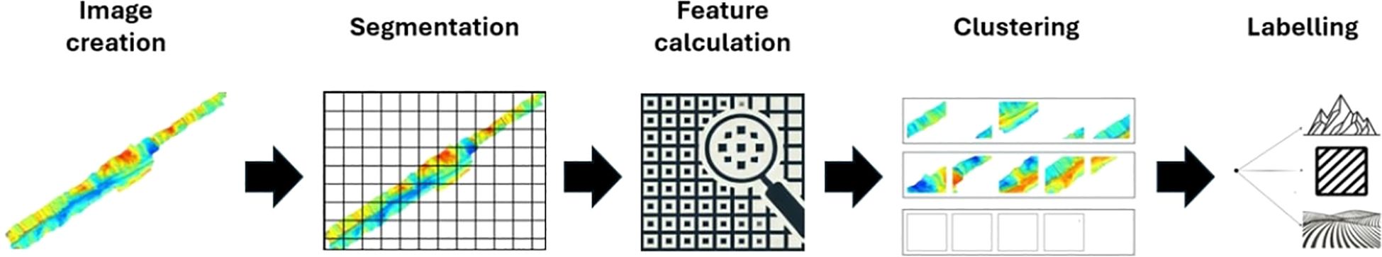
Figure 1. Workflow for filtering images containing potential small seamounts from multibeam bathymetric data. The process involves five key steps: (1) creation of a high-resolution seafloor map, (2) segmentation into smaller images for efficient processing, (3) feature extraction using CNNs, (4) filtering of images based on calculated feature vectors, and (5) manual labeling of filtered images to identify potential seamount candidates for further analysis.
Image Creation: The input consists of multibeam bathymetric data that has been preprocessed to correct artifacts and improve overall quality. To ensure clean input data, outlier detection and removal were performed using the optimized filtering method described by Ziolkowski et al. (2024), which enhances data reliability by eliminating spurious depth values from multibeam echo-sounder measurements. High-resolution seafloor maps were subsequently generated using Python’s Matplotlib library, applying the viridis color scheme to represent depth variations. This perceptually uniform colormap enhances contrast between flat seafloor and elevated features such as seamounts, facilitating the ability of the U-Net architecture to learn and distinguish relevant morphological patterns during the segmentation process. To ensure that every 256×256 image uses the same absolute depth-to-color mapping (and thus identical contrast), we compute a single pair of “global” depth limits (global min, global max) over the entire input survey before tiling. After interpolating each 24×24 chunk and resizing it to 256×256, we clip every pixel to [global min,global max] and linearly rescale to [0,1]. In this way, no two images from the same survey ever have different contrast ranges—each pixel’s color always maps back to the same meter-value. Segmentation: To efficiently manage the computational challenges of seafloor mapping, the data is divided into 256 × 256 pixel images with 10% overlap, ensuring that no seamount is truncated at the segment edges. This step enables efficient downstream processing while retaining critical morphological details in each region and ensuring that the image size is large enough to fully visualize entire seamount structures. We chose 256 × 256 as our image size because it is a common power-of-two input for U-Net. We briefly tested 128 × 128 (faster but lost small-feature fidelity) and 512 × 512 (higher fidelity but 4× more memory/time) and found that 256 × 256 provided the best trade-off. Pixel resolution is kept fixed across all surveys: each chunk is first interpolated to a 24 × 24 grid at 0.001° resolution—covering 0.024° × 0.024° in latitude/longitude—and then resized to 256 × 256 pixels. Hence each pixel corresponds to 9.375 × 10° (10 m, depending on latitude), both during training and application. Even if a new dataset has different raw point densities, our pipeline “forces” it onto that same 0.024°footprint per image, so the model always sees a consistent meter-per-pixel scale. In summary, by fixing grid resolution=0.001 and chunk size=24 and always resampling to 256 × 256, we guarantee identical pixel resolution from training to application, regardless of which survey file is used. Feature Calculation: CNNs compute feature vectors for each segmented image, capturing key characteristics such as texture and structure. These vectors provide a compact, descriptive representation of the seafloor features, enabling effective analysis.
Clustering: Feature vectors are clustered into 10 groups using unsupervised methods, which ensures that images with similar morphological characteristics are grouped together, significantly reducing dataset complexity and focusing attention on potential seamount regions. The choice of k=10 was not arbitrary but reflects a balance between two competing needs: capturing the major morphological variations in our CNN-derived feature space and keeping the number of clusters low enough for efficient human review. In practice, we found that ten clusters cleanly separated large, flat or gently sloping patches from steeper, seamount-like textures. Increasing k beyond 10 rarely produced qualitatively new seamount candidate groups—most extra clusters simply subdivided empty or flat-area images—while fewer than ten clusters began to merge distinct seamount morphologies with background.
Labeling: A domain expert reviews and labels the clusters. This human oversight ensures accurate identification of potential seamount candidates. Images of flat seafloor and background are excluded from further analysis, while the potential seamount cluster is retained for subsequent steps. On average, the cluster-level review takes under five minutes per survey: the expert scans a handful of thumbnails from each of the 10 clusters (100 images total) in about 2–3 minutes, discards the clearly “background” clusters, and flags only a few as “seamount candidates.” If desired, they can then page through those candidate clusters for extra confidence—but the minimal filtering step is complete in under five minutes, since no individual “yes/no” decision is made on all 5–804 images. The result of this methodology is a refined dataset of labeled clusters. Only the clusters containing potential seamounts undergo further analysis to detect the summits and extents of each seamount.
3.2 Workflow for training and evaluating a CNN for seamount detection
The workflow shown in Figure 2 outlines the process for preparing, training, and evaluating a UNet architecture to detect seamounts in multibeam data, beginning after the pre-selection of images likely to contain seamounts (Figure 1). Data Input: The workflow starts with the selected images containing regions that most likely include seamounts, as shown in Figure 2. These images serve as the input for the subsequent labeling and model training steps.
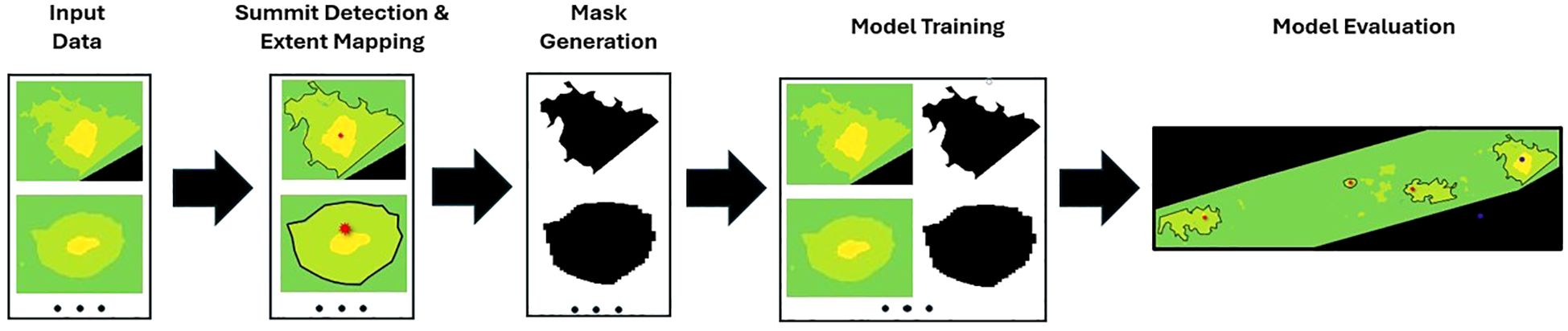
Figure 2. Workflow illustrating the processing pipeline for training a UNet architecture to detect small seamounts in multibeam data. The pipeline begins with raw multibeam data input, followed by extent mapping to annotate seamount features. Masks are then generated to prepare training images, which are used to train the UNet model. The workflow concludes with model evaluation to assess performance and accuracy in detecting and delineating seamounts.
Summit Detection and Extent Mapping: Using labelme, seamount features are manually annotated to create masks for training. Black polygons outline the extent of each seamount. This step ensures accurate identification of key morphological features essential for the training process. Although all annotations were created by a single domain expert to maintain consistency, this introduces potential subjectivity and bias into the ground truth masks. Future work should consider inter-annotator agreement studies or collaborative labeling strategies to better quantify annotation reliability and improve robustness of training data.
Mask Generation: The annotated summit and extent data are used to generate binary masks for each seamount, where black areas represent the seamount and white areas indicate the background. These masks serve as the ground truth for training the UNet architecture, establishing the expected output for each input image.
Model Training: The UNet architecture is trained using the input images and their corresponding masks. The model learns to map the input image features to the expected output, enabling it to detect and delineate seamounts in multibeam bathymetric data accurately.
Model Evaluation: The trained model is evaluated using the mean Intersection over Union (mean IoU) metric, which measures the overlap between the predicted and manually labeled masks and ranges from 0 (no overlap) to 1 (perfect overlap). A higher mean IoU indicates better model performance in identifying and segmenting seamounts, providing a reliable assessment of its accuracy. Generally, mean IoU values between 0.75 and 0.85 are considered acceptable for complex medical segmentation tasks, particularly when segment boundaries are difficult to define, such as in tumor segmentation or vessel segmentation (Amri et al., 2025; Peng et al., 2025; Moradmand and R, 2025). In addition to mean IoU, the Dice coefficient is another widely used metric in image segmentation, particularly in medical imaging. It measures the similarity between predicted and ground-truth segmentations and ranges from 0 (no overlap) to 1 (perfect overlap). The Dice coefficient is particularly useful in imbalanced datasets, where positive class pixels (e.g., segmented structures) are much fewer than background pixels (Chamseddine et al., 2025; Yang et al., 2025; Alyahyan, 2025).
To optimize model training, the Dice loss function is employed, which is derived from the Dice coefficient. It is commonly used in medical image segmentation because it mitigates the effect of class imbalance by emphasizing the similarity of foreground structures rather than treating all pixels equally. Dice loss is especially beneficial for detecting small and irregularly shaped structures, making it a suitable choice for seamount segmentation, where feature boundaries are often ambiguous (Zhang et al., 2025; Shen et al., 2025). In future studies, implementing cross-validation labeling rounds with multiple annotators and calculating inter-annotator metrics such as Cohen’s kappa (Cohen, 1960) could further strengthen the training dataset quality and reduce the likelihood of label noise.
This workflow represents a comprehensive pipeline for training and evaluating a UNet model tailored for the automatic detection of small seamounts. It combines human expertise in labeling with advanced machine learning techniques, enabling efficient and accurate analysis of multibeam bathymetric data.
4 Results and discussion
4.1 Analysis of model performance in seamount image filtering using feature vectors
Seamount images show complex patterns and structural ambiguity, posing significant challenges for automated feature extraction. The results indicate that models with stronger feature extraction capabilities, such as VGG16 and ResNet50, produced more precise feature vectors, leading to better clustering performance and higher agreement with manual labeling.
Models that rely on lightweight architectures and reduced feature complexity, such as MobileNetV2, demonstrated lower performance, particularly in separating clusters when faced with highly uneven cluster sizes. InceptionV3, while effective in capturing variations in shape and color, exhibited reduced clustering precision when confronted with uniform textures across different clusters. Below, the performance of each model is discussed in terms of cluster separation, agreement with manual labeling, strengths, and weaknesses, as summarized in Table 1.
● VGG16: VGG16 achieved the highest agreement with manual labeling (97–100%), demonstrating robust and interpretable feature extraction, leading to clear cluster separation. Its architecture is particularly suited to datasets with clear patterns, making it ideal for applications requiring consistent and robust feature extraction. However, its tendency to over represent large clusters limited its effectiveness for highly complex or imbalanced datasets.
● ResNet50: ResNet50 performed well in scenarios requiring the extraction of more complex or abstract patterns, achieving 81–90% agreement with manual labeling. It is a viable alternative for datasets with higher structural variability or subtle morphological differences. However, its performance was less consistent than VGG16, particularly in datasets with limited textural differentiation, where it struggled to maintain stable clustering.
● InceptionV3: InceptionV3 showed strong multi-scale feature extraction but lower consistency, with agreement scores ranging from 66–94%. It is recommended for datasets with significant variability in patterns and colors, but it is less effective for uniform image distributions. Its performance was hindered when dealing with color homogeneity within clusters, leading to occasional misclassification.
● MobileNetV2: MobileNetV2 had the lowest agreement with manual labeling (18–82%), reflecting its difficulty in handling fine-grained textures and separating clusters effectively. This was especially evident in datasets where clusters varied significantly in size, ranging from single instances to over 3000 images. While computationally efficient, MobileNetV2 should be avoided in tasks requiring detailed feature extraction, such as seamount identification, due to its inability to handle complex patterns.
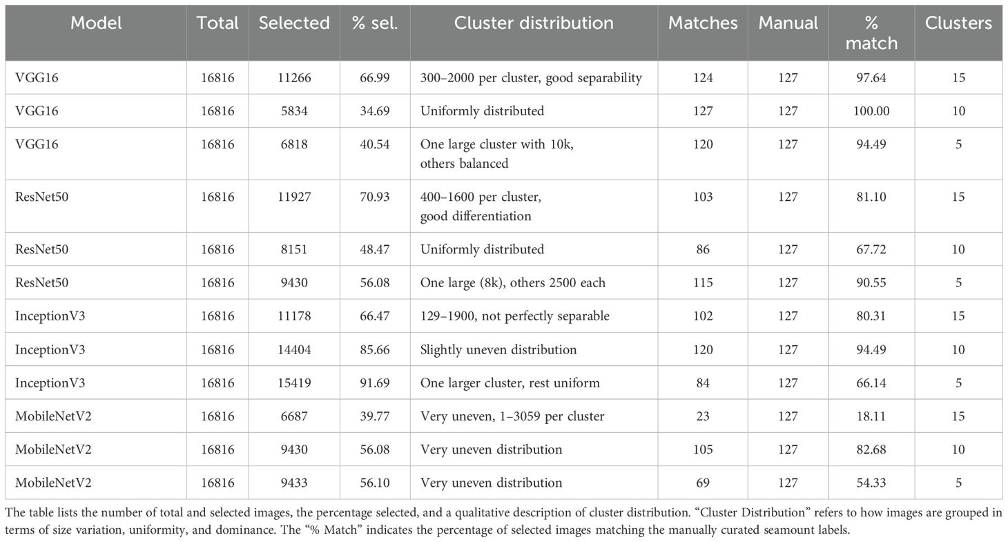
Table 1. Summary of clustering results across different CNN architectures for seamount image classification.
The analysis highlights VGG16 as the optimal model for seamount identification due to its ability to extract robust features and achieve high agreement with manual labeling. ResNet50 is a strong alternative for datasets with complex patterns but suffers from inconsistencies in cluster separation. InceptionV3 is useful for datasets with diverse features but struggles with uniform patterns, while MobileNetV2 is unsuitable for this application due to its limited feature extraction capabilities and poor clustering performance. These insights provide a clear basis for selecting appropriate models based on the specific requirements of seamount image clustering tasks.
4.2 Training of the U-Net architecture for seamount detection
The dataset used for training the U-Net architecture consists of high-resolution bathymetric and geological data collected during two research cruises, MSM75 and MSM88, in the Atlantic Ocean. These datasets provide detailed information on seafloor morphology, fault structures, and small seamounts, making them well-suited for an image-based deep learning approach.
The MSM75 cruise, conducted in 2018, focused on four key areas along the Reykjanes Ridge, a slows preading ridge influenced by the Iceland hotspot. This dataset includes 15 m resolution ship-based bathymetry, ROV-based ground-truthing, and geochemical analyses of glass samples, capturing variations in magma composition, fault density, and seamount morphology. These features are strongly influenced by factors such as distance from the hotspot and the magmatic or tectonic accretion state of axial volcanic ridges (AVRs) (Le Saout et al., 2023). Given the distinct geological and morphological variations within the dataset, it provides an excellent basis for training a segmentation model capable of distinguishing complex seafloor structures.
Complementing this, the MSM88 cruise dataset, collected using a Kongsberg EM 122 multibeam system at approximately 100 m horizontal resolution, covers a much larger area—approximately 153,121 square kilometers—spanning from the Cabo Verde Exclusive Economic Zone (EEZ) to the EEZs of Guadeloupe, Dominica, and Martinique. This dataset includes diverse Atlantic seabed morphologies, ranging from flat sedimented plains to seamounts, fracture zones, and the Mid-Atlantic Ridge. The large volume of depth soundings (86 million) ensures high spatial coverage and variability, further enhancing the robustness of the training data.
Table 2 provides an overview of the spatial extent, resolution, and depth ranges of the three datasets used for training and testing. The diversity of these datasets enhances the robustness and applicability of the model across different seafloor morphologies.
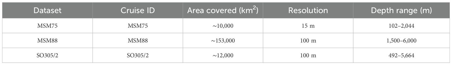
Table 2. Summary of bathymetric datasets used for training and evaluation.
These datasets are particularly well-suited for training the U-Net model, as they provide high-resolution seafloor imagery with detailed geological labels. The combination of fine-scale bathymetry from MSM75 and the broader regional coverage of MSM88 ensures that the model learns to generalize across varying seafloor structures, improving its ability to segment and classify geological features effectively.
4.3 Hyperparameter selection and training strategy
In this section, we analyze the impact of different hyperparameter configurations on the performance of the U-Net architecture for seamount detection. The evaluation focuses on validation loss, mean Intersection over Union (IoU), and validation mean IoU, as summarized in Table 3. The goal of this analysis is to identify the optimal parameter constellation for final model training, ensuring high segmentation accuracy and robustness.
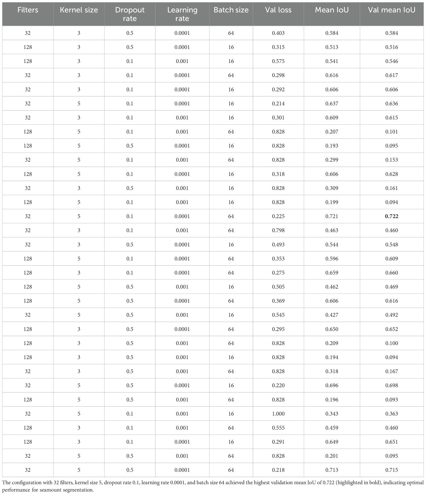
Table 3. Hyperparameter tuning results for U-Net.
Mean Intersection over Union (IoU) is a widely used metric in image segmentation, quantifying the overlap between predicted and ground truth masks. It is calculated as the ratio of the intersection to the union of both masks, ranging from 0 to 1, where higher values indicate better segmentation performance (Dwarakanath and Kuntiyellannagari, 2025).
Several key hyperparameters were varied during the grid search, including the number of filters, kernel size, dropout rate, learning rate, and batch size. One of the primary considerations is the number of filters in the convolutional layers, which defines the depth of feature extraction. A lower filter count, such as 16, may fail to capture sufficient spatial details, whereas a significantly higher count, such as 256 or more, increases computational costs and the risk of overfitting, particularly given the relatively small dataset size. To balance feature richness and computational efficiency, 32 and 128 filters were selected, following insights from prior research in biomedical segmentation tasks (Iqbal et al., 2022; Srinivasan et al., 2024).
Another crucial factor is the kernel size, which determines the receptive field of convolutional layers. Smaller kernels, such as 3 × 3, are effective for fine-grained detail extraction, while larger kernels, such as 5 × 5, allow for broader spatial pattern detection in bathymetric structures. The study focused on comparing these two kernel sizes, as excessively large kernels (e.g., 7 × 7) could introduce computational challenges and potentially over-smooth small-scale features.
To mitigate overfitting and enhance generalization, dropout rate was varied between 0.1 and 0.5. Dropout serves as a regularization technique by randomly deactivating neurons during training, preventing the model from relying too heavily on specific features. This variation allowed for an assessment of the trade-off between preventing overfitting and ensuring sufficient information retention for effective segmentation.
Additionally, the learning rate plays a vital role in determining how quickly the model updates its weights during training. A low learning rate encourages stable convergence, whereas a higher learning rate accelerates training but increases the risk of overshooting optimal weight values. To identify an optimal balance, the study compared learning rates of 0.0001 and 0.001, ensuring that the model could learn effectively without instability or divergence. We use the Adam optimizer (with the learning rate chosen via our hyperparameter search). Adam combines the benefits of momentum and adaptive learning rates, which helps stabilize training on our relatively small U-Net dataset.
Lastly, the batch size was explored to assess its effect on training efficiency and model performance. Smaller batch sizes allow for more frequent weight updates per iteration, while larger batch sizes contribute to more stable gradient estimations. To maintain a balance between computational efficiency and convergence stability, batch sizes of 16 and 64 were evaluated.
Their selection was guided by best practices in deep learning, computational efficiency, and the unique characteristics of bathymetric data. Specifically, the dataset was divided into 80% training and 20% validation sets using stratified sampling to preserve class balance and ensure a robust evaluation of model performance. We combined labeled images from both MSM75 and MSM88 into a single pool, then applied an 80/20 split with random state=42, so the training/validation split is fixed across all runs. For augmentation, we rotated each normalized 256×256 image by 90° and 180°, producing two extra images per original (three total). These practices are widely adopted in the geospatial and marine sciences communities and have been recommended for applications involving multibeam bathymetry and habitat mapping (Summers et al., 2021; Roelfsema et al., 2021). Their influence on model performance is analyzed in the following sections, with a focus on preventing overfitting and supporting generalization across diverse seafloor morphologies.
The following sections discuss the results of these hyperparameter configurations, analyzing their influence on model performance and the trade-offs they introduce in the context of seamount segmentation.
4.3.1 Number of filters
In our implementation, the number of filters doubles at each successive “down” step in the encoder and then halves again in the decoder. The results indicate that models using 32 filters generally outperform those with 128 filters in terms of mean IoU and validation mean IoU. The best-performing configuration (32 filters, kernel size 5, dropout rate 0.1, learning rate 0.0001, batch size 64) achieves a validation mean IoU of 0.722, higher than configurations with 128 filters, which generally yield IoU values below 0.66.
Models with 128 filters and a large kernel size (5) tend to perform poorly, particularly in cases where the dropout rate is high or the learning rate is large. Several configurations with 128 filters, kernel size 5, dropout rate 0.5, and a learning rate of 0.001 resulted in extremely poor performance (mean IoU < 0.21). These results suggest that larger models may overfit or fail to generalize when handling small-scale features in seamount detection.
4.3.2 Kernel size
A kernel size of 5 consistently improves model performance compared to a kernel size of 3. The best-performing models all use a 5 × 5 kernel, which appears to enhance the model’s ability to capture seamount structures in multibeam data. Notably, the highest validation mean IoU (0.722) is obtained with a 5 × 5 kernel, 32 filters, dropout rate 0.1, learning rate 0.0001, and batch size 64.
Configurations with a 3 × 3 kernel tend to yield slightly lower performance, with validation mean IoU values ranging from 0.584 to 0.660. While smaller kernels may still be effective, the data suggests that capturing larger contextual information with a 5 × 5 kernel improves segmentation quality. Larger kernels (e.g., 7 × 7) were not tested due to increased computational complexity and potential over-smoothing of small seamount features.
4.3.3 Dropout rate
The best-performing models use a dropout rate of 0.1, while higher dropout rates (0.5) lead to a decline in performance. Configurations with dropout 0.5 frequently result in unstable training, with validation mean IoU values dropping below 0.55 in most cases. This suggests that excessive regularization hinders the network’s ability to learn fine-grained features necessary for segmenting small seamounts. Lower dropout values (<0.1) were avoided to prevent potential overfitting, while higher values (>0.5) were not considered due to excessive information loss during training.
4.3.4 Learning rate
A learning rate of 0.0001 is generally more stable and results in higher mean IoU values than 0.001. Many configurations with a learning rate of 0.001 exhibit poor performance, with validation loss values reaching 0.828, indicating divergence or unstable training.
Notably, when a learning rate of 0.0001 is used in combination with a kernel size of 5 and dropout rate of 0.1, the model achieves the best performance. These findings suggest that a lower learning rate prevents the model from overshooting optimal weights, leading to better generalization. Higher learning rates (>0.01) were excluded due to the risk of divergence, while lower rates (<0.0001) were avoided as they could lead to excessively slow training.
4.3.5 Batch size
The best-performing models generally use a batch size of 64. While some configurations with batch size 16 perform well (validation mean IoU around 0.66), they do not outperform batch size 64 when combined with optimal hyperparameters.
Interestingly, several models with batch size 16 and 128 filters perform significantly worse, possibly due to instability in training. A larger batch size appears to contribute to better gradient estimation and stable convergence. Extremely large batch sizes (>128) were not tested due to GPU memory constraints and the risk of poor generalization.
4.3.6 Optimal configuration and conclusions
Based on this analysis, the best-performing configuration is:
32 filters, kernel size 5, dropout rate 0.1, learning rate 0.0001, batch size 64.
This configuration achieves the highest validation mean IoU of 0.722, suggesting that it provides the most reliable segmentation performance for small seamounts. These results emphasize the importance of choosing a balanced architecture that prevents overfitting while ensuring stable learning dynamics. The findings also reinforce that hyperparameter tuning is essential for optimizing deep learning models in seamount segmentation, as poor configurations can severely impact model accuracy and generalization ability.
4.3.7 Balancing generalization and model complexity
In deep learning applications, particularly those involving image segmentation, managing the balance between model complexity and generalization is crucial to avoid overfitting or underfitting. These phenomena directly influence a model’s ability to perform accurately on unseen data and are especially critical when working with spatially diverse and sparsely labeled bathymetric datasets.
Overfitting occurs when a model learns the training data too well, including its noise and minor fluctuations, leading to poor generalization on validation or test data. This typically manifests as a low training loss combined with a high validation loss. In contrast, underfitting arises when the model is too simplistic to capture the underlying patterns of the data, resulting in high errors on both training and validation sets.
To ensure that the U-Net model maintains a strong balance between learning capacity and generalization, we monitored validation loss, mean Intersection over Union (IoU), and validation mean IoU across training epochs (see Table 3). These metrics help assess both segmentation accuracy and model robustness. In particular, consistently high validation mean IoU values without significant divergence from training performance indicate strong generalization ability.
Additionally, to avoid overfitting, regularization strategies such as dropout, early stopping, and data augmentation were applied. Stratified sampling was used to divide the dataset into 80% training and 20% validation subsets, preserving class balance and ensuring that all seamount categories are proportionally represented.
The observed performance trends align with best practices established in machine learning literature. For example, Sivakumar et al. (2024) emphasize the trade-off between training and testing ratio and its effect on generalization in image processing. Similarly, Manikandan et al. (2024) highlight the impact of architectural complexity on overfitting and underfitting in segmentation tasks using U-Net, supporting our methodological choices for small seamount detection.
While the model demonstrates strong validation performance, a limitation remains its sensitivity to out-of-domain (OOD) data—bathymetric inputs that differ significantly from the training distribution in terms of seafloor morphology, resolution, or noise characteristics. Such domain shifts frequently occur in real-world deployments and may degrade model reliability. Future work should therefore explore strategies such as domain adaptation, transfer learning, and uncertainty quantification. These approaches can improve robustness by enabling the model to generalize to morphologically diverse regions, reducing the risk of false positives or negatives in unfamiliar tectonic settings. Transfer learning, in particular, has shown promise in segmentation tasks with sparse annotations and heterogeneous data domains, such as in medical imaging (Tajbakhsh et al., 2016).
4.4 Application of workflow to real-world data
The data shown in Figure 3 were acquired during SO305-2, a transit across the Indian Ocean after exiting the territorial waters of Indonesia and Malaysia. Using the EM122 swath mapping system, high-resolution bathymetric data were collected along this tectonically active region, which exhibits significant deformation of the oceanic plate. The dataset reveals detailed seafloor morphology, uncovering previously uncharted geological features in this underexplored area.
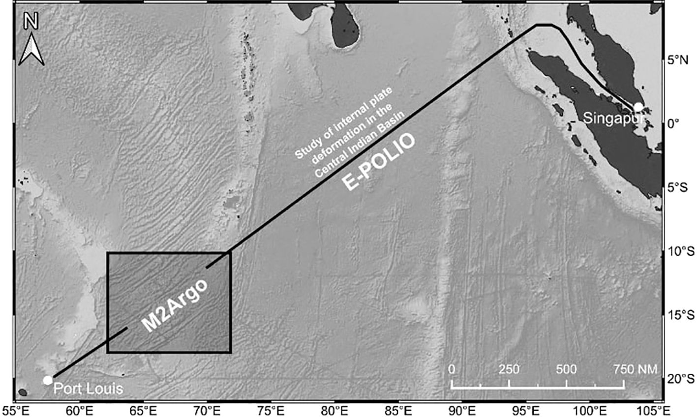
Figure 3. Joint working area of the E-POLIO and M2Argo projects during the SO305–2 cruise, shown along the transit route from Singapore to Port Louis. The boxed area indicates the survey region focused on the ARGO fracture zone.
As the survey approached the Central Indian Ridge (CIR), it focused on the Argo transform fault and its fracture zones. The EM122 system detected numerous small seamounts, many less than 1000 meters in diameter, which remain undetectable in lower-resolution satellite altimetry. This highlights the limitations of satellite-based mapping for smaller topographic features and underscores the advantages of multibeam systems in resolving fine-scale bathymetric details.
This high-resolution dataset provides a valuable resource for developing and validating automated seamount detection algorithms. It offers detailed bathymetric imagery across varied tectonic settings, making it an ideal testbed for refining detection methods and improving our understanding of small seamount distribution and morphology.
A total of 11,139 images were generated from the SO305–2 expedition data during preprocessing, with 30 seamounts manually labeled. To prepare the dataset for seamount detection, a filtering and clustering process (Section 4.1) reduced the dataset to 6,626 images, effectively eliminating 40% of the original data. As shown in Figure 4, clusters 1, 6, and 7 were selected for further processing, as they most likely contain seamount images, while the remaining clusters primarily represent flat seafloor or other irrelevant features. Clusters 0 and 2, identified as potential artifacts likely caused by noise, were excluded from further analysis. Additionally, 30 seamounts were manually identified within the dataset, and all 30 seamounts from the original data were retained in the selected images, ensuring comprehensive coverage of the target structures for model training. For model training, we used the 256×256 images generated from the MSM75 and MSM88 datasets, in which 138 seamounts had been manually labeled. The U-Net was trained on this combined pool of MSM75/MSM88 images.
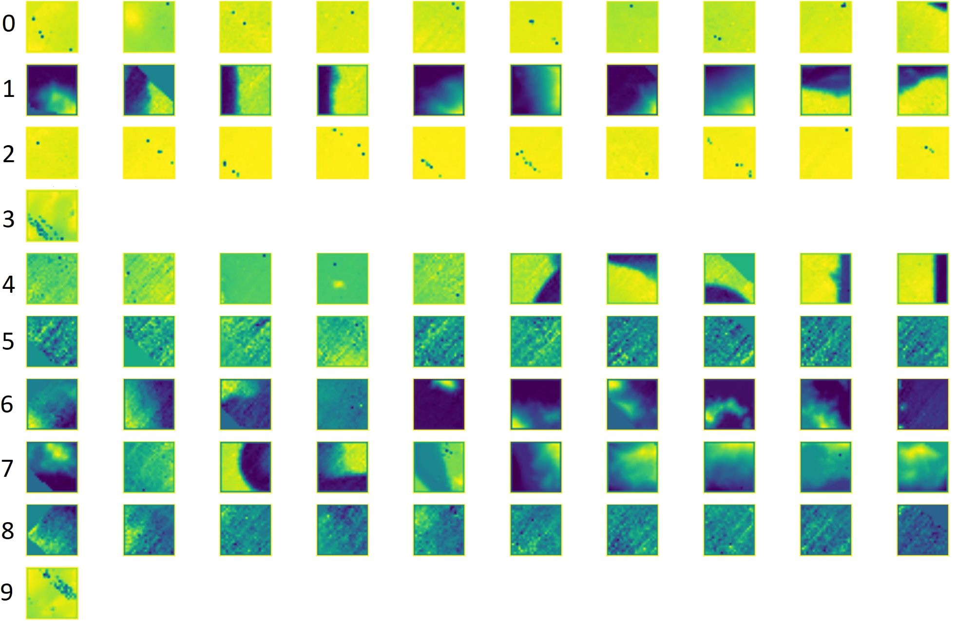
Figure 4. Clusters generated after the filtering process, highlighting distinct seafloor morphologies. Clusters 1, 6, and 7 likely contain seamount images, making them suitable for further analysis. All other clusters primarily represent flat seafloor or similar features and can be excluded from the U-Net detection process for small seamount detection.
The model was trained using the optimal hyperparameters identified in Section 4.3. To prevent overfitting and ensure optimal performance, early stopping was implemented, monitoring validation loss and halting training once no further improvements were observed. Additionally, model checkpointing was used to save the model whenever a lower validation loss was achieved, ensuring retention of the best-performing version for further evaluation. The progression of validation loss throughout training is shown in Figure 5, exhibiting a steady decline until approximately epoch 37, after which further reductions become minimal.
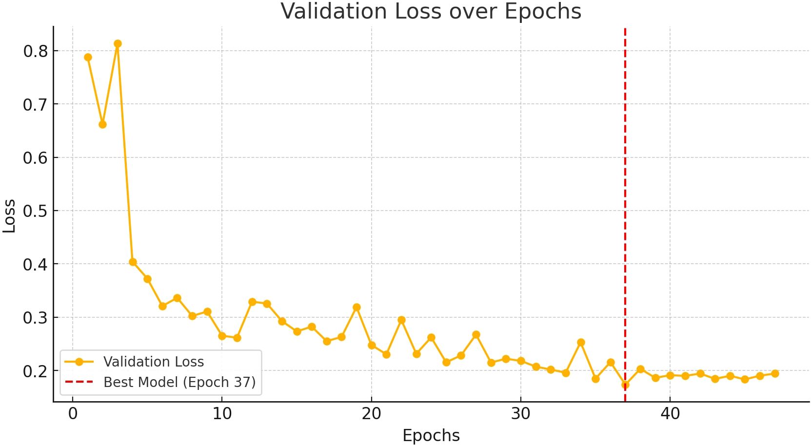
Figure 5. Validation loss over epochs during model training. The red dashed line indicates the epoch where the best model was saved based on the lowest validation loss.
Throughout training, the model demonstrated a progressive improvement in segmentation performance, as reflected in the increasing Dice Coefficient and Mean IoU, while validation loss steadily decreased. Dice Loss, commonly used in segmentation tasks to mitigate class imbalance, is derived from the Dice Coefficient, a similarity measure evaluating the overlap between two sets. As for class imbalance, most images have no seamount pixels, and even in images that do, seamounts cover only about 10–20% of pixels—hence our use of Dice Loss. By emphasizing misclassified regions, Dice Loss helps capture fine-grained structures, making it particularly effective for segmenting objects with irregular boundaries (Zheng et al., 2025).
During the initial training phase (epochs 1–10), the model exhibited low Dice scores, ranging from approximately 0.14 to 0.21. However, validation loss dropped sharply from 0.85 to 0.26 within this period, with the first major performance improvement occurring around epoch 5, marking the transition to more stable learning. This trend is illustrated in Figure 6, which depicts the evolution of the Dice Coefficient over epochs.
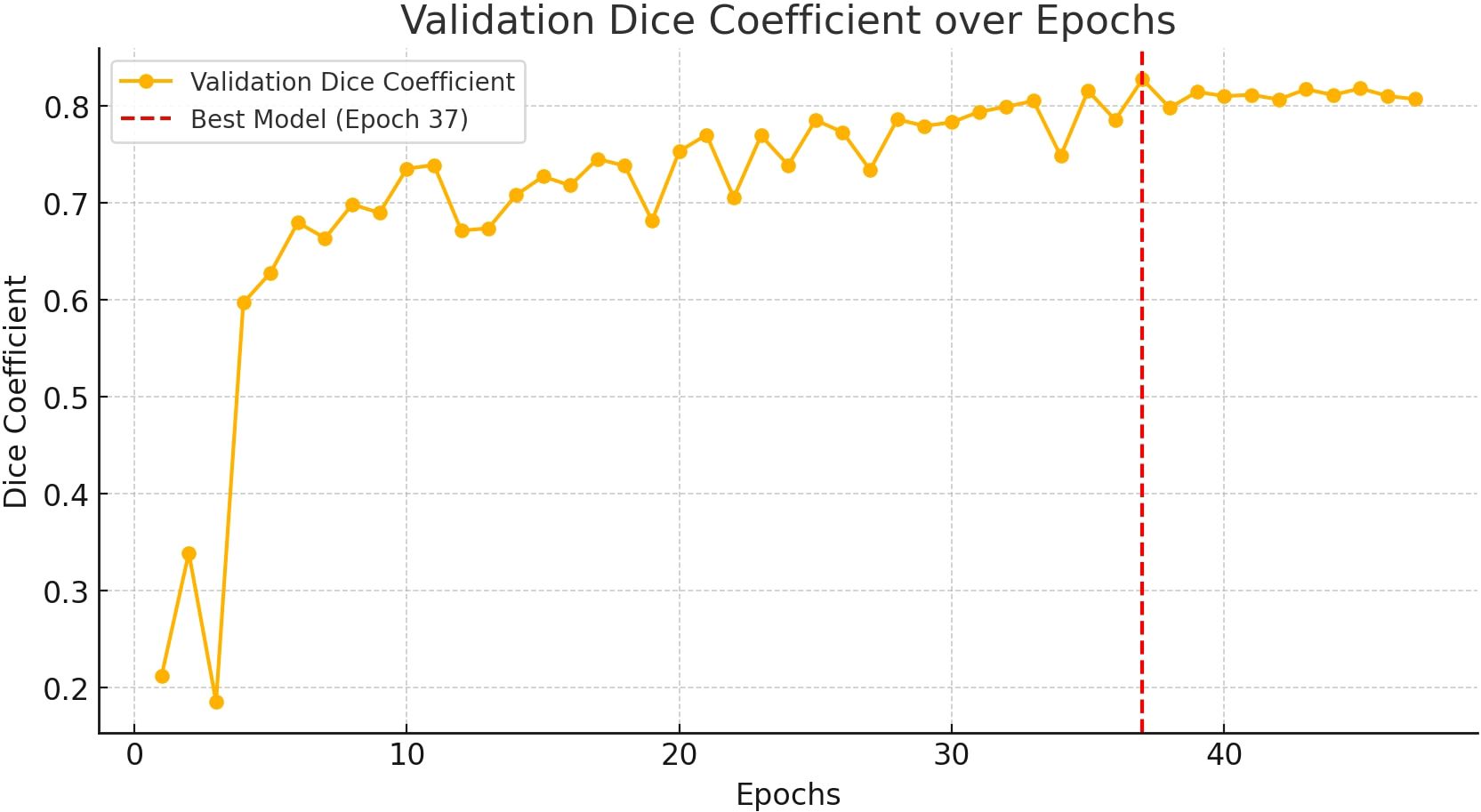
Figure 6. Validation Dice coefficient over epochs. A higher Dice coefficient indicates better segmentation performance. The red dashed line highlights the best model.
In the mid-training phase (epochs 11–30), the model continued improving, with validation loss reaching its minimum (0.1734) at epoch 37. The Dice Coefficient rose significantly, surpassing 0.82, while the Mean IoU exhibited a steady upward trend, further indicating the model’s ability to generalize effectively. The trajectory of the Mean IoU over training epochs, as visualized in Figure 7, reflects this improvement.
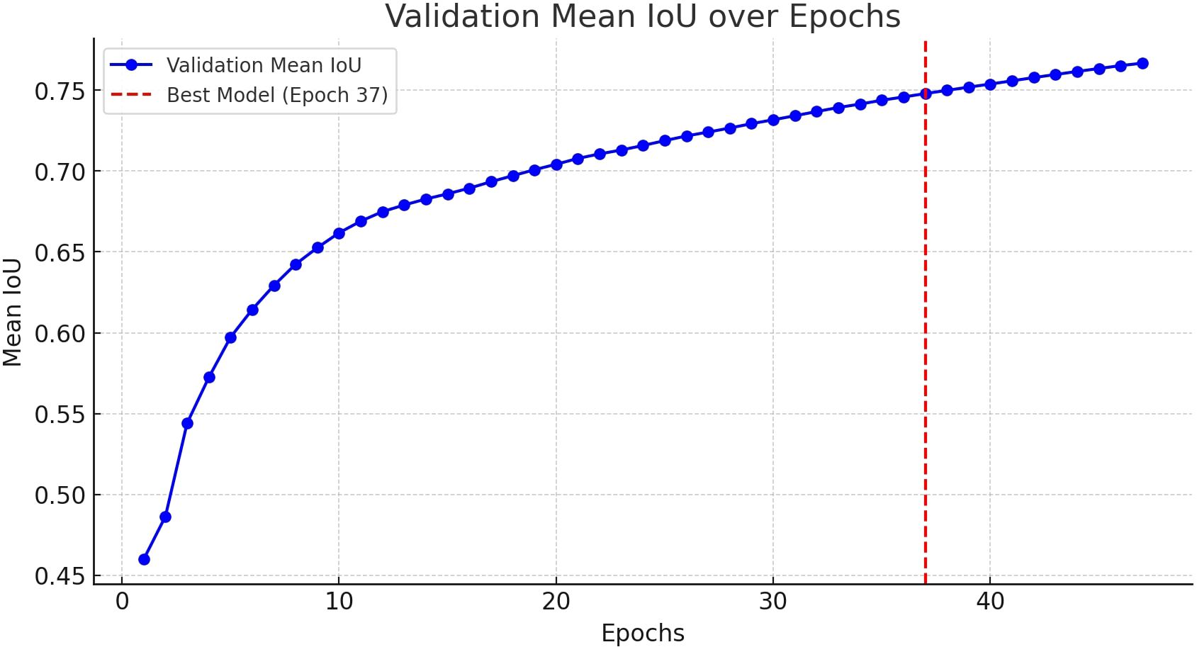
Figure 7. Validation mean Intersection over Union (IoU) over epochs. The IoU metric evaluates the overlap between predicted and ground truth segmentation masks, with higher values indicating better performance.
During the late training phase (epochs 30–50), signs of overfitting emerged as validation loss plateaued. The Dice Coefficient fluctuated between 0.81 and 0.86, while the Mean IoU remained relatively stable, showing minimal gains beyond epoch 37. These observations suggest that further training did not yield additional benefits, indicating that the model had reached its optimal performance.
The best performance was recorded at epoch 37, where validation loss reached its minimum (0.1734), and the model attained a Dice Coefficient of 0.8274 and a Mean IoU of 0.7514—representing the peak segmentation accuracy observed during training. These results suggest that the model successfully learned meaningful feature representations for image segmentation, with performance stabilizing beyond this epoch. Consequently, epoch 37 was identified as the optimal balance point between learning and generalization.
After training, the U-Net model was applied to the filtered dataset to generate segmentation results for seamount detection. Model predictions were compared to manually labeled seamounts to assess performance. The U-Net successfully identified all 30 seamounts in the dataset, demonstrating high detection accuracy. The predicted outlines closely matched the ground truth, with only minor deviations in shape and boundary precision, suggesting that the model effectively captures key morphological characteristics of seamounts.
Figure 8 displays all 30 manually labeled seamounts alongside their corresponding model predictions, highlighting the robustness of the proposed workflow in accurately detecting and segmenting small seamount structures.
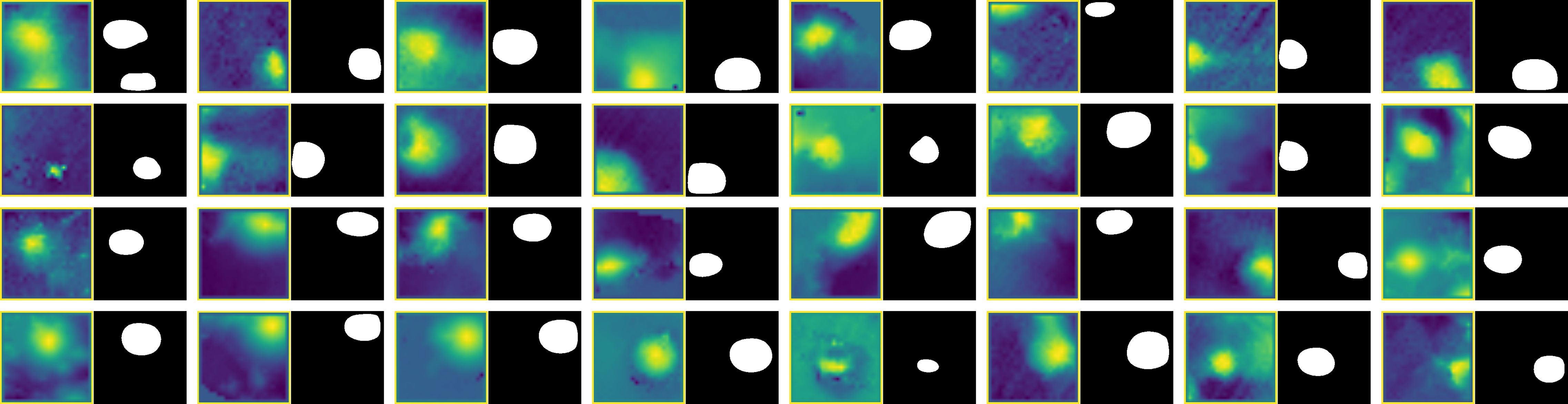
Figure 8. Comparison of manually selected images containing seamounts and their corresponding U-Net model predictions. The predicted seamounts closely align with the actual seamount locations, indicating the model’s high detection performance.
To further illustrate the challenges of detecting small seamounts, Figure 9 presents examples of false predictions made by the U-Net model. The misclassification of certain regions as seamounts can be attributed to the complexity of seafloor morphology and the inherent subjectivity of manual labeling. Seafloor features vary significantly, and even human interpreters may disagree on what qualifies as a seamount. Given this subjectivity, discrepancies between model predictions and reference labels are expected due to human error or differing interpretations of the data.
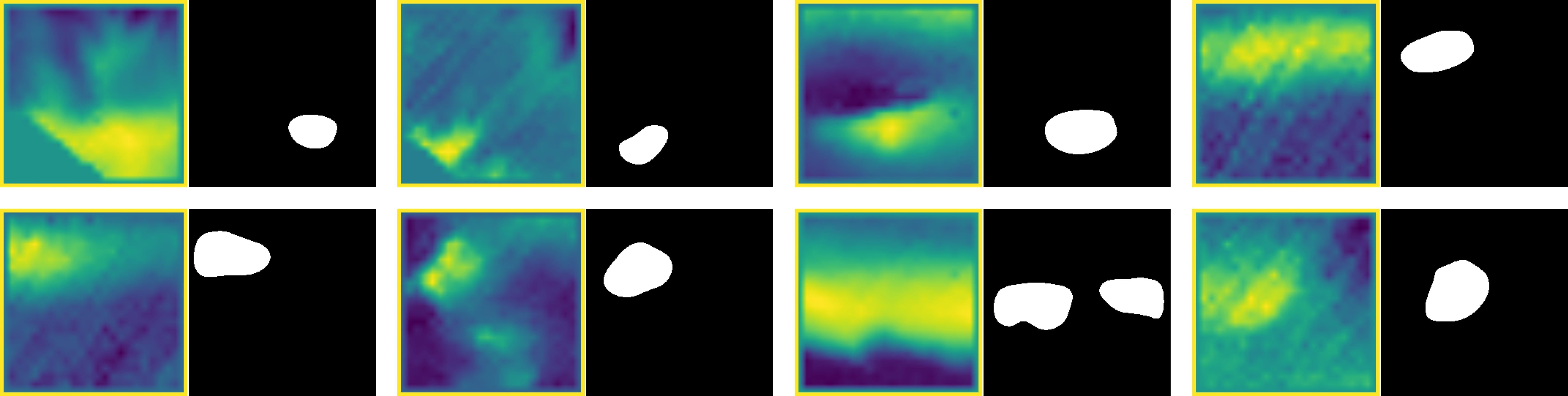
Figure 9. Examples of false predictions made by the U-Net model. In these cases, the model incorrectly labeled certain seafloor features as seamounts, likely due to local elevation changes or elongated structures that share some morphological characteristics with true seamounts. These misclassifications highlight the challenges in distinguishing small seamounts from other topographic variations in bathymetric data.
A common characteristic among false positives is the presence of localized seafloor elevations, which appear as yellow regions in the bathymetric data. Although not actual seamounts, these features share topographic similarities with true seamount structures, making misclassification understandable. However, a key limitation of the U-Net model is its occasional inability to accurately capture the typical circular morphology of small seamounts. Instead, elongated or irregularly shaped elevations are sometimes misclassified as seamounts despite lacking the distinct topographic characteristics that define them.
These observations suggest that while the model effectively identifies seafloor elevations, it could be further improved in distinguishing true seamounts from other raised features. Future refinements could involve integrating morphological constraints during training or applying post-processing techniques to filter out elongated structures that do not conform to the expected circular shape of small seamounts.
In Section 2, this study identified three key challenges in small seamount detection: (1) the scarcity of manually labeled training data, (2) the difficulty of segmenting irregular and morphologically diverse features, and (3) the need for models that generalize across varying seafloor conditions. To address the first challenge, a training set of 138 seamounts was manually labeled using high-resolution multibeam bathymetry, providing a diverse and representative dataset for supervised learning. The second challenge was mitigated through the use of the U-Net architecture, whose encoder-decoder structure and skip connections allow for precise pixel-wise segmentation of irregular and fine-scale seafloor features. Lastly, the model’s generalization capability was enhanced by filtering the dataset with a CNN-based clustering approach, reducing noise and guiding the network’s attention to relevant regions. Together, these strategies enabled effective training and application of a robust segmentation model capable of detecting small seamounts with high accuracy in real-world data.
Figure 10 highlights the 30 seamounts identified in the SO305–2 dataset, revealing a significant number of previously undetected features. A major limitation of satellite-derived global seamount datasets, such as those based on vertical gravity gradient (VGG) data, is their inability to resolve smaller seamounts (Yesson et al., 2011). Consequently, only 14 of the 30 identified seamounts were visible in satellite altimetry data, while the remaining 16 were too small to be detected. This underscores the importance of high-resolution.
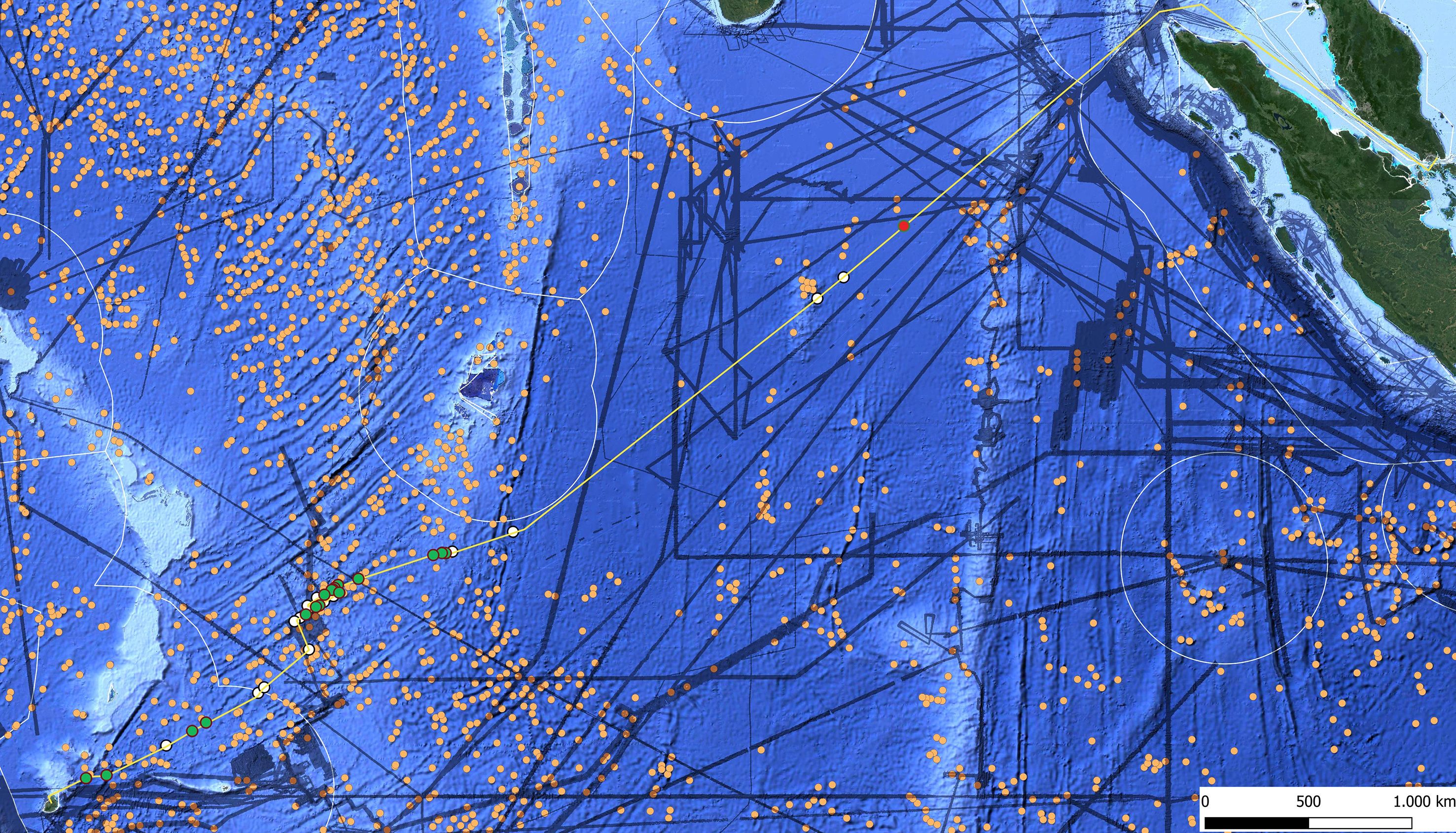
Figure 10. Map showing the 30 seamounts identified during the SO305/2 expedition. Seamounts detected by our model and also reported by Gevorgian et al. (2023) and Kim and Wessel (2011) are marked in white. Green dots indicate newly discovered seamounts that were not previously documented, while the red dot represents a location where a seamount was expected based on Gevorgian et al. (2023) and Kim and Wessel (2011), but no actual seamount was found. These findings highlight the effectiveness of multibeam systems in detecting previously unknown seamounts. The expedition started in Singapore (top right) and concluded in Mauritius (bottom left).
As shown in Table 4, 16 of the 30 identified seamounts (well-known = 2) were completely absent from global satellite datasets. In their study, Gevorgian et al. (2023) improved upon previous altimetry-based seamount detection methods, identifying seamounts as small as 421 meters in height, with most detections exceeding 700 meters due to the limitations of the VGG method. This marked a significant improvement over earlier studies, such Kim and Wessel (2011), who noted that traditional altimetry-based methods struggled to detect features smaller than 1,500 meters due to the limited resolution of gravity anomaly data. These findings underscore the limitations of satellite-derived data in detecting smaller seamounts and highlight the necessity of high-resolution multibeam bathymetric surveys for comprehensive seafloor mapping.
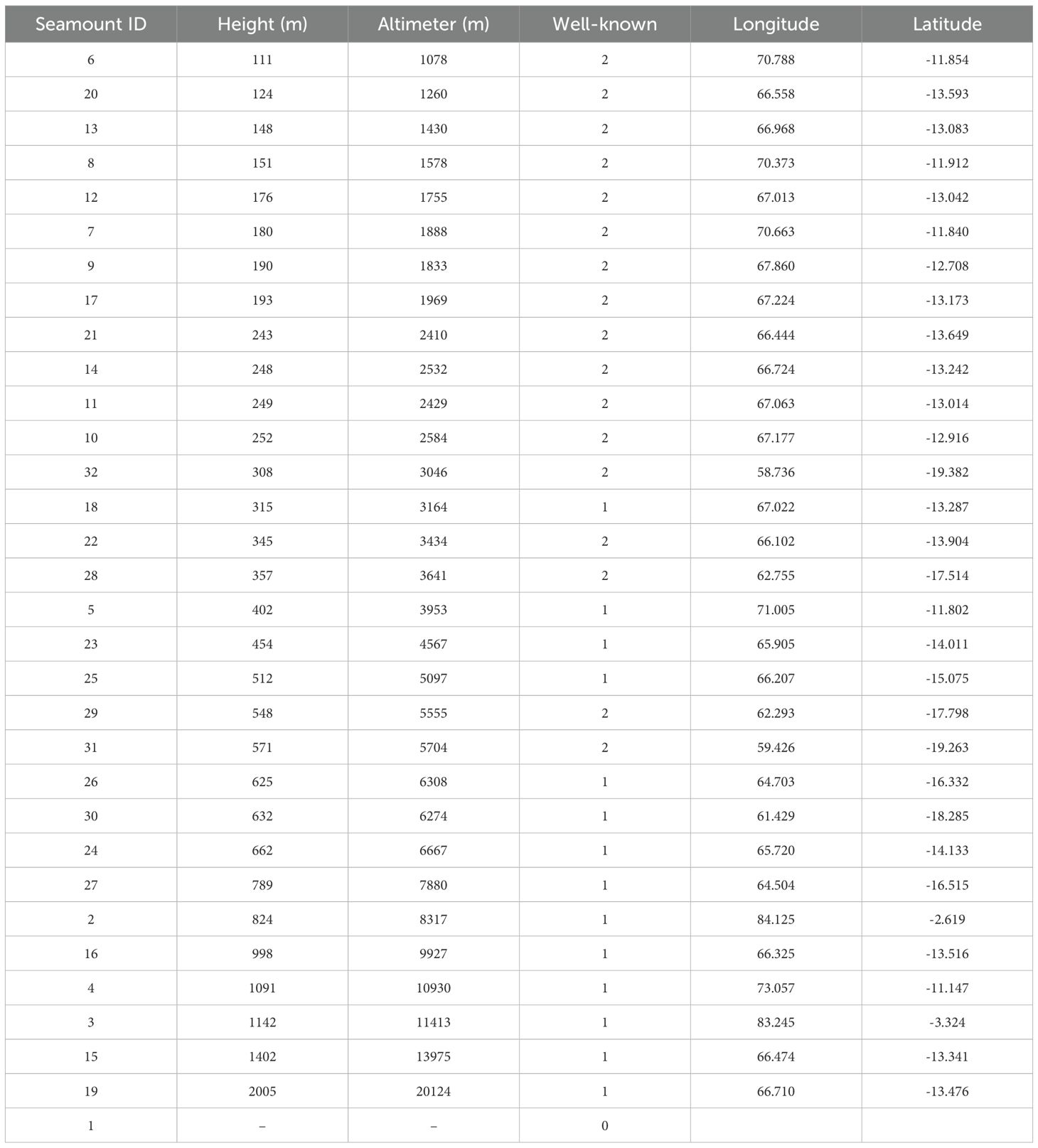
Table 4. Seamount characteristics including height, altimeter-derived height, well-known status, and coordinates.
Additionally, 10 seamounts (well-known = 1) were previously cataloged by Gevorgian et al. (2023) and Kim and Wessel (2011), but our method provided independent validation of their existence using direct multibeam observations. These seamounts, ranging from 315 to 2,005 meters in height, demonstrate that our approach can both confirm and refine existing seamount inventories through high-precision bathymetric measurements.
Interestingly, one feature predicted in previous seamount catalogs (well-known = 0) was not confirmed in our multibeam dataset. This discrepancy suggests a false positive in the satellite-derived data, potentially caused by noise, interpolation artifacts, or misclassification of other seafloor features as seamounts. Such cases highlight the importance of direct validation using high-resolution mapping to ensure the accuracy of global seamount databases.
Overall, these findings emphasize the crucial role of multibeam sonar in capturing fine-scale seafloor topography and identifying small seamounts that remain undetected in satellite altimetry data. While altimetry-based methods provide valuable large-scale global coverage, they systematically underestimate the number of small seamounts due to resolution constraints. By applying machine learning-based segmentation on high-resolution bathymetry, our approach bridges the gap between broad-scale satellite surveys and precise, localized mapping techniques.
5 Conclusion
This study introduced a deep-learning-based framework for detecting small seamounts in multibeam bathymetric data, addressing key limitations of traditional classification methods and satellite altimetry. The proposed two-step approach—combining CNN-based filtering with U-Net segmentation—significantly improved detection accuracy and efficiency. The findings provide insights into each of the research questions posed in the introduction:
● How does a filtering-based approach improve the identification of small seamounts in multibeam bathymetric data compared to direct classification methods? The results demonstrated that CNNbased filtering enhances seamount detection by pre-selecting relevant image subsets, reducing noise and improving segmentation accuracy. Unlike direct classification methods, which attempt to classify entire images, the filtering process focuses only on regions likely to contain seamounts, reducing false positives and computational complexity. This two-step strategy outperformed traditional direct classification methods, ensuring that the segmentation model processes only meaningful data.
● What are the optimal hyperparameters for training a U-Net model to achieve the highest segmentation accuracy for small seamount detection? A grid search analysis identified the best-performing hyperparameter configuration: 32 filters, a kernel size of 5 × 5, a dropout rate of 0.1, a learning rate of 0.0001, and a batch size of 64. These settings balanced feature extraction depth, regularization, and training stability, yielding the highest segmentation accuracy, with a Dice Coefficient of 0.8274 and a Mean IoU of 0.7514. Models with excessively high filter counts or dropout rates exhibited overfitting or unstable convergence, highlighting the need for a balanced architecture in seamount segmentation tasks.
● How well does the proposed framework generalize across different geographic regions, and what limitations arise when applying a model trained in one ocean basin to another? While the model performed well on the SO305–2 dataset, cross-regional generalization remains a challenge. When tested on new datasets, the model maintained high accuracy for seamounts with well-defined topographic signatures, but performance declined in regions with highly variable seafloor morphology. This suggests that further fine-tuning or domain adaptation strategies may be necessary when applying the model to seamounts formed under different tectonic and geological conditions.
● To what extent can satellite altimetry reliably detect small seamounts, and how do its results compare to high-resolution multibeam bathymetric data? The results confirmed that satellite altimetry systematically underestimates the number of small seamounts due to resolution constraints. Of the 30 seamounts detected in the SO305–2 dataset, only 14 were visible in satellite-derived data, highlighting the importance of high-resolution multibeam bathymetry for capturing fine-scale seafloor features. Additionally, satellite-derived databases contained false positives, underscoring the need for direct validation using multibeam sonar.
Beyond geological applications, the automated detection of seamounts has broader implications for marine ecology, environmental monitoring, and plate tectonics research. Future work should focus on improving cross-regional generalization, integrating morphological priors into deep-learning models, and expanding the dataset to further enhance classification accuracy. In addition, improving the annotation process through inter-annotator validation or collaborative labeling could reduce subjectivity and improve the reliability of training labels, which is particularly important in seafloor datasets where feature boundaries can be ambiguous. In particular, the integration of domain adaptation or transfer learning methods holds promise for improving model performance in morphologically diverse or OOD seafloor regions, enabling broader applicability of the framework without requiring extensive manual relabeling or retraining. To further enhance robustness in real-world applications, future models should also incorporate strategies for handling OOD inputs, including uncertainty estimation and domain-specific priors to reduce prediction errors in unfamiliar seafloor environments. By bridging the gap between machine learning and marine geosciences, this framework contributes to the advancement of automated seafloor mapping and global seamount inventories, improving our understanding of the ocean floor.
Data availability statement
The datasets presented in this study can be found in online repositories. The names of the repository/repositories and accession number(s) can be found below: https://doi.pangaea.de/10.1594/PANGAEA.972385.
Author contributions
TZ: Formal analysis, Visualization, Investigation, Validation, Writing – review & editing, Software, Writing – original draft, Conceptualization, Methodology. CD: Investigation, Writing – review & editing, Validation, Supervision, Conceptualization. AK: Validation, Investigation, Supervision, Writing – review & editing.
Funding
The author(s) declare financial support was received for the research and/or publication of this article. We acknowledge the financial support provided by MarDATA — Helmholtz School for Marine Data Science, Germany for this research project. We thank Captain Bjorn¨ Maaß and Captain Oliver Meyer and their crew for support at sea while collecting the training data set. I additionally want to thank the GEOMAR Open Access Publikationsfonds for providing support for the publication fee.
Conflict of interest
The authors declare that the research was conducted in the absence of any commercial or financial relationships that could be construed as a potential conflict of interest.
Generative AI statement
The author(s) declare that Generative AI was used in the creation of this manuscript. Solely for text correction and language refinement. All scientific content, analyses, and interpretations were developed by the author(s) without the aid of generative AI.
Publisher’s note
All claims expressed in this article are solely those of the authors and do not necessarily represent those of their affiliated organizations, or those of the publisher, the editors and the reviewers. Any product that may be evaluated in this article, or claim that may be made by its manufacturer, is not guaranteed or endorsed by the publisher.
References
Alyahyan S. (2025). A novel nemonet framework for enhanced rcc detection and staging in ct images. Discov. Comput. 28, 4. doi: 10.1007/s10791-025-09499-0
Amri Y., M Z., S R., and Slama A. B. (2025). Automatic glioma segmentation based on efficient u-net model using mri images. Artif. Intelligence-Based. Med. 11, 100216. doi: 10.1016/j.ibmed.2025.100216
Chamseddine E., Tlig L., and Sayadi M. (2025). Gabrain-net: An optimized gabor-integrated u-net for multimodal brain tumor mri segmentation. Brain Tumor. MRI. Segment. - SSRN. doi: 10.2139/ssrn.5105664
Chen L.-C., Zhu Y., Papandreou G., Schroff F., and Adam H. (2018). “Encoder-decoder with atrous separable convolution for semantic image segmentation,” in Proceedings of the European Conference on Computer Vision (ECCV), 801–818. doi: 10.1007/978-3-030-01234-249
Cherubini C., Piazzolla D., and Saccotelli L. (2024). Habitat suitability modeling of loggerhead sea turtles in the central-eastern mediterranean sea: a machine learning approach using satellite tracking data. Front. Mar. Sci 11. doi: 10.3389/fmars.2024.1493598
Chitre V., Nashipudmath M. M., and Shinde S. (2024). Exploring machine learning techniques for predictive analytics in computational mathematics. Comput. Math. J. doi: 10.52783/pmj.v34.i2.919
Clark M. R., S T., and Rowden A. A. (2010). The ecology of seamounts: Structure, function, and human impacts. Annu. Rev. Mar. Sci. 2, 253–278. doi: 10.1146/annurev-marine-120308-081109
Cohen J. (1960). A coefficient of agreement for nominal scales. Educ. psychol. Measure. 20, 37–46. doi: 10.1177/001316446002000104
Cracknell M. J. and Reading A. M. (2014). Geological mapping using remote sensing data: A comparison of five machine learning algorithms, their response to variations in the spatial distribution of training data and the use of explicit spatial information. Comput. Geosci. 63, 22–33. doi: 10.1016/j.cageo.2013.10.008
Deng S., Ning D., and Mayon R. (2024). The motion forecasting study of floating offshore wind turbine using self-attention long short-term memory method. Ocean. Eng. 310, 2024. 127899. doi: 10.1016/j.oceaneng
Dwarakanath B. and Kuntiyellannagari B. (2025). Glioma segmentation using hybrid filter and modified african vulture optimization. Bull. Electric. Eng. Inf. 14, 2. doi: 10.11591/eei.v14i2.8730
Gevorgian J., Sandwell D. T., Yu Y., Kim S.-S., and Wessel P. (2023). Global distribution and morphology of small seamounts. Earth Space. Sci. 10, e2022EA002331. doi: 10.1029/2022EA002331
He K., Gkioxari G., Dollár P., and Girshick R. B. (2017). “Mask r-cnn,” in Proceedings of the IEEE International Conference on Computer Vision (ICCV) (IEEE), 2961–2969. doi: 10.1109/ICCV.2017.322
He K., S. R., Zhang X., and Sun J. (2016). “Deep residual learning for image recognition,” in Proceedings of the IEEE Conference on Computer Vision and Pattern Recognition (CVPR), 770–778. doi: 10.1109/CVPR.2016.90
Huang D. X., W. G., W. X., W. W., and Sun Y. F. (2024). Research on seamount substrate classification method based on machine learning. Front. Mar. Sci. 11. doi: 10.3389/fmars.2024.1431688
Iqbal A., Sharif M., Khan M. A., Nisar W., and Alhaisoni M. (2022). Ff-unet: a u-shaped deep convolutional neural network for multimodal biomedical image segmentation. Cogn. Comput. 14, 1563–1579. doi: 10.1007/s12559-022-10038-y
Jones D. O. B., D. A. B. B., and Simon-Lledó E. (2021). Environment, ecology, and potential effectiveness of an area protected from deep-sea mining (clarion clipperton zone, abyssal pacific). Prog. Oceanogr. 197, 102653. doi: 10.1016/j.pocean.2021.102558
Khalil S. M., Haywood E., and Forrest B. (2024). Standard Operating Procedures for Geoscientific Data Management, Louisiana Sand Resources Database (LASARD) (Louisiana: Tech. rep., Coastal Protection and Restoration Authority of Louisiana).
Kim S.-S. and Wessel P. (2011). New global seamount census from altimetry-derived gravity data. Geophys. J. Int. 186, 615–631. doi: 10.1111/j.1365-246X.2011.05076.x
Le Saout M., Pałgan D., Devey C. W., Lux T. S., Petersen S., Thorhallsson D., et al. (2023). Variations in volcanism and tectonics along the hotspot-influenced reykjanes ridge. Geochem. Geophys. Geosyst. 24, e2022GC010788. doi: 10.1029/2022GC010788
Liu A., Liu Y., Xu K., Zhao F., and Zhou Y. (2024). Deepseanet: A bio-detection network enabling species identification in the deep sea imagery. IEEE Trans. Geosci. Remote Sens. 62, 1–13. doi: 10.1109/TGRS.2024.10415449
Manikandan J., Harini K., and Saranya M. (2024). “Deep learning-based lung cancer detection and classification with hybrid sampling for imbalanced data,” in 2024 International Conference on Smart Technologies (IEEE).
Matabos M., J S., and Barreyre T. (2022). Integrating multidisciplinary observations in vent environments (imove): Decadal progress in deep-sea observatories at hydrothermal vents. Front. Mar. Sci. 9. doi: 10.3389/fmars.2022.866422
Mitchell N. C. (2001). Transition from circular to stellate forms of submarine volcanoes. J. Geophys. Res.: Solid. Earth 106, 1987–2003. doi: 10.1029/2000JB900263
Moradmand H. and R L. (2025). Multistage deep learning methods for automating radiographic sharp score prediction in rheumatoid arthritis. Sci. Rep. 15, 3391. doi: 10.1038/s41598-025-86073-0
Peng M., Y. W., Q. M., T. W., and Li J. (2025). Accurate and robust segmentation of cerebral distal small arteries by dvnet with dual contextual path and vascular attention enhancement. Quant. Imaging Med. Surg. 15, 2. doi: 10.21037/qims-24-1514
Qin X., L X., S J., Z D., Z J., and Wu Z. (2024). Musrfm: Multiple scale resolution fusion-based precise and robust satellite derived bathymetry model for island nearshore shallow water regions. ISPRS. J. Photogramm. Remote Sens. 128, 150–169. doi: 10.1016/j.isprsjprs.2024.09.007
Roelfsema C. M., Lyons M., Murray N., and Phinn S. R. (2021). Workflow for the generation of expert-derived training and validation data: A view to global scale habitat mapping. Front. Mar. Sci. 8. doi: 10.3389/fmars.2021.643381
Ronneberger O., Fischer P., and Brox T. (2015). “U-net: Convolutional networks for biomedical image segmentation,” in Medical Image Computing and Computer-Assisted Intervention – MICCAI 2015. Eds. Navab N., Hornegger J., Wells W. M., and Frangi A. F. (Springer International Publishing, Cham), 234–241.
Sandler M., M. Z. A. Z., Howard A., and Chen L.-C. (2018). “Mobilenetv2: Inverted residuals and linear bottlenecks,” in Proceedings of the IEEE Conference on Computer Vision and Pattern Recognition (CVPR), 4510–4520. doi: 10.1109/CVPR.2018.00474
Shen Y., J. L., H. C., C. W., H. D., and Chen L. (2025). Pads-net: Gan-based radiomics using multi-task network of denoising and segmentation for ultrasonic diagnosis of parkinson disease. Med. Imaging Anal. 120, 102490. doi: 10.1016/j.compmedimag.2024.102490
Simonyan K. and Zisserman A. (2015). “Very deep convolutional networks for large-scale image recognition,” in International Conference on Learning Representations (ICLR).
Sivakumar M., Parthasarathy S., and Padmapriya T. (2024). Trade-off between training and testing ratio in machine learning for medical image processing. PeerJ. Comput. Sci. 10, e2245. doi: 10.7717/peerj-cs.2245
Smith D. K. (1988). Shape analysis of pacific seamounts. Earth Planet. Sci. Lett. 90, 457–466. doi: 10.1016/0012-821X(88)90143-4
Srinivasan S., Durairaju K., Deeba K., Mathivanan S. K., Vijayakumar M., and Murugan P. (2024). Multimodal biomedical image segmentation using multi-dimensional u-convolutional neural network. BMC Med. Imaging 24, 1–17. doi: 10.1186/s12880-024-01197-5
Summers G., Lim A., and Wheeler A. J. (2021). A scalable, supervised classification of seabed sediment waves using an object-based image analysis approach. Remote Sens. 13, 2317. doi: 10.3390/rs13122317
Szegedy C., S. I.-J. S., Vanhoucke V., and Wojna Z. (2016). “Rethinking the inception architecture for computer vision,” in Proceedings of the IEEE Conference on Computer Vision and Pattern Recognition (CVPR), 2818–2826. doi: 10.1109/CVPR.2016.308
Tajbakhsh N., Shin J. Y., Gurudu S. R., Hurst R. T., Kendall C. B., Gotway M. B., et al. (2016). Convolutional neural networks for medical image analysis: Full training or fine tuning? IEEE Trans. Med. Imaging 35, 1299–1312. doi: 10.1109/TMI.2016.2535302
Usui A. and S K. (2022). Geological characterization of ferromanganese crust deposits in the nw pacific seamounts for prudent deep-sea mining. Deep-Sea. Mining.: Sustainabil. Technol. Environ. Issues. 81–113. doi: 10.1007/978-3-030-87982-24
Valentine A. P. and Kalnins L. M. (2013). Discovery and analysis of topographic features using learning algorithms: A seamount case study. Geophys. Res. Lett. 40, 3596–3600. doi: 10.1002/grl.50615
Wang C.-Y. H.-Y. M. L. and Bochkovskiy A. (2022). Yolov7: Trainable bag-of-freebies sets new state-of-the-art for real-time object detectors. arXiv. preprint. doi: 10.48550/arXiv.2207.02696
Yang J., H. W., Y. L., Y. S., X. F., and Huang S. (2025). A novel 3d lightweight model for covid-19 lung ct lesion segmentation. Med. Eng. Phys. 137, 104297. doi: 10.1016/j.medengphy.2025.104297
Yesson C., Clark M. R., Taylor M., and Rogers A. D. (2011). The global distribution of seamounts based on 30-second bathymetry data. Deep. Sea. Res. Part I.: Oceanogr. Res. Papers. 58, 442–453. doi: 10.1016/j.dsr.2011.02.004
Zhang L., X Z., and Zhang W. (2025). Automatic liver tumor segmentation based on improved yolo-v5 and b-spline level set. Cluster. Comput. 28, 214. doi: 10.1007/s10586-024-04918-1
Zheng Y., Tian B., Yu S., Yang X., Yu Q., and Zhou J. (2025). Adaptive boundary-enhanced dice loss for image segmentation. Biomed. Signal Process. Control. 106, 107741. doi: 10.1016/j.bspc.2025.102526
Keywords: multibeam, seamount, convolutional neural network, seamount catalog, feature vector, bathymetry, U-net, seafloor mapping
Citation: Ziolkowski T, Devey CW and Koschmider A (2025) Detecting small seamounts in multibeam data using convolutional neural networks. Front. Mar. Sci. 12:1613061. doi: 10.3389/fmars.2025.1613061
Received: 16 April 2025; Accepted: 21 July 2025;
Published: 15 August 2025.
Edited by:
Muhammad Yasir, China University of Petroleum (East China), ChinaReviewed by:
Peter Feldens, Leibniz Institute for Baltic Sea Research (LG), GermanyArthur C. Trembanis, University of Delaware, United States
Copyright © 2025 Ziolkowski, Devey and Koschmider. This is an open-access article distributed under the terms of the Creative Commons Attribution License (CC BY). The use, distribution or reproduction in other forums is permitted, provided the original author(s) and the copyright owner(s) are credited and that the original publication in this journal is cited, in accordance with accepted academic practice. No use, distribution or reproduction is permitted which does not comply with these terms.
*Correspondence: Tobias Ziolkowski, dHppb2xrb3dza2lAZ2VvbWFyLmRl