Abstract
Introduction:
Fish keypoint detection is a prerequisite for accurate fish behavior analysis and biomass weight estimation, and is therefore crucial for efficient and intelligent offshore aquaculture. Traditional keypoint detection networks typically employ coordinate regression methods, which do not impose any constraints on the output of the regression head or the training process of the neural network. As a result, output keypoints of such networks do not always conform to the shape of a fish and the training process can be affected by incorrect labels, leading to errors in subsequent tasks.
Methods:
To address these issues, this paper proposes a robust deep learning approach characterized by three improvements. 1) A shape model of fish that includes the average shape of fish, principal components of fish keypoints, and corresponding eigenvalues is constructed using principal component analysis (PCA) and unscented transform. 2) A customized version of anchor boxes is introduced and referred to as “anchor fish”, which along with the shape model, can be used to encode and decode fish keypoints. 3) Shape variation loss, calculated based on the eigenvalues in the shape model, is added as part of the loss function to constrain the output of the regression head. Moreover, we built a fish keypoint dataset using infrared cameras mounted on a truss-structure net cage.
Results and discussion:
Comparative experiments on our dataset using the keypoint evaluation method from COCO are conducted. The results show that our method achieves an AP50 value of 0.656, significantly outperforming the well-designed YOLO5Face, which produces an AP50 value of 0.503. Furthermore, we have comprehensively explored the impact of key hyperparameters on detection performance and robustness to labeling outliers in the training set. The code is available at https://github.com/LMX-BY/fish_landmark_detection_using_PCA_based_fish_shape_model.
1 Introduction
Computer vision is gaining popularity in offshore aquaculture, driven by its ability to enable long-term, automated monitoring and data analysis for aquaculture processes (Yang et al., 2021). One of the key challenges in aquaculture that computer vision aims to address is fish keypoint detection. This task involves identifying the two-dimensional coordinates of semantic points on a fish, such as the head, the tail, and the fins, in images, and determining which points belong to the same individual. Unlike object detection, which outputs bounding boxes ( (Zou et al., 2023), keypoint detection provides more granular information for aquaculture applications. By analyzing keypoints, it is possible to estimate both the size and quantity of fish, as well as more sophisticated tasks such as motion tracking and behavior analysis (Zhao et al., 2021).
Fish keypoints detection depends on careful sensor selection and placement, as well as effective algorithm design. Typically, fish images are captured using either underwater cameras (Labao and Naval, 2019; Salman et al., 2020) or above-water cameras (Li et al., 2022; Han et al., 2020). Underwater cameras, despite their ability to capture close-up images, have significant practical limitations, including a narrow field of view, poor image quality, and a tendency to biofouling, which necessitates frequent cleaning and results in high maintenance costs (Reyes et al., 2020; Salama et al., 2018). In contrast, our setup employs above-water infrared cameras (Li et al., 2024), offering a wider field of view, clearer images, and insensitivity to lighting conditions, all while minimizing maintenance costs. This configuration is particularly well-suited for long-term monitoring of fish species that exhibit nocturnal water-surface activity, such as the Cobia (Rachycentron canadum).
Keypoint detection algorithms vary based on the application scenario, such as human keypoint detection (also known as pose estimation), which involves significant occlusion and variations in shape and appearance. Therefore, it is common to use heat maps as outputs to represent the position distribution of each keypoint. Those algorithms can be categorized into two main approaches: top-down (Newell et al., 2016; Wei et al., 2016; He et al., 2017; Sun et al., 2019) and bottom-up (Newell et al., 2017; Cheng et al., 2020; Li et al., 2020). The top-down approach begins by employing an object detection method to identify individual objects, followed by extracting keypoints from the image patches that contain these objects. This approach is particularly well-suited for situations where the objects are sparsely distributed. The bottom-up approach first detects keypoints and then assembles those keypoints into individuals, making it highly effective for both small-scale objects and densely populated scenes. At the same time, to extract more representative features, various network structures and training methods have been proposed. By introducing the idea of multi-stage feature extraction (Ramakrishna et al., 2014) into deep learning, stacked hourglass network (Newell et al., 2016) are proposed. This network aggregate multiple lightweight networks with down-sampling and up-sampling processes to learn multi-scale spatial relationships between keypoints, thereby improving accuracy. Xiao et al. (2018) designed a simple and single-stage network structure, referred to as SimpleBaseline, which utilizes ResNet as the backbone and incorporates a single down-sampling and up-sampling network to output high-resolution heat maps. Their reported accuracy surpasses that of Stacked Hourglass Networks. To further improve the efficiency of SimpleBaseline, Zhong et al. (2021) proposed a lightweight up-sampling unit and deep supervision pyramid architecture. Li et al. (2019) analyzed the reasons for the lower accuracy observed in multi-stage methods compared to single-stage methods and suggested improvement strategies, such as adopting more sophisticated single-stage modules and coarse-to-fine supervision training.
Another typical scenario is facial keypoint detection. Given that the face occupies a relatively small portion of an image, heatmap based outputs are not necessarily required. Before the advent of deep learning, a common approach was to formulate facial keypoint detection as an optimization problem (Saragih et al., 2011; Cao et al., 2014), where parameters such as scaling, rotation, translation, and Point Distribution Model (PDM)-based shape coefficients (Cootes and Taylor, 1992) were optimized. The loss function was composed of both shape and keypoint appearance losses. Another notable method (Kazemi and Sullivan, 2014) attempted to learn an ensemble of regression trees as a cascade of regression functions to achieve super-real-time performance. Building on deep learning features, Baltrusaitis et al. (2013) introduce a keypoint appearance loss and propose a non-uniform regularized keypoint mean-shift algorithm to solve the optimization problem for keypoint alignment. However, complex scenarios with varying lighting, shape, and viewpoint have exposed the limitations of these carefully designed methods. In contrast, end-to-end deep learning-based keypoint detection has demonstrated superior performance. Yashunin et al. (2020) introduce the MaskFace, which is very similar to Mask R-CNN, with the key difference being that it employs a one-stage object detection network. RetinaFace (Deng et al., 2019) extends a typical target detection network by adding a regression head, which directly translates the feature vector at the corresponding image location to keypoint coordinates. Additionally, an FPN and a context module are integrated to extract and aggregate multi-scale image features, further enriching the network’s representation capabilities. Building on YOLOv5, Qi et al. (2022) introduced several key improvements, including the adoption of Wing Loss (Feng et al., 2018) as the cost function for keypoint regression and the utilization of ShuffleNetV2 as the backbone network, thereby achieving a balance between speed and accuracy.
Deep learning-based algorithms have also been applied to improve the performance of fish keypoints detection. A prevalent approach is the top-down approach (Dong et al., 2023; Wu et al., 2022; Suo et al., 2020), which yields better results when combined with advanced object detection networks and keypoint regression networks, such as YOLOv5 and Lite-HRNet. Yu et al. (2023) designed a bottom-up keypoint regression network. Unlike the usual approach of directly regressing keypoints, this network integrates the heatmap of keypoints, the offset of the target center, and the size of the target in the head. However, the authors did not provide the advantages of this approach. For scenarios where only a single fish is present in an image, Saleh et al. (2023) designed a lightweight network, MFLD-net, which can be deployed on low-cost devices. Kumar et al. (2022) compared the heatmap-based method with the coordinate-regression method and concluded that the heatmap-based approach using U-Net architecture performs better.
Analysis of existing methods reveals that both heatmap-based and coordinate regression-based methods lack explicit constraints on the distribution of output keypoints, potentially resulting in invalid shapes. Taking fish keypoints as an example, the four keypoints of a typical fish should follow a specific distribution. As shown in Figure 1, both sets of keypoints on the left and right sides consist of four points each, yet the keypoints on the left form valid fish shapes, whereas those on the right represent impossible combinations.
Figure 1

A schematic diagram of fish shapes composed of four keypoints. The left column shows valid fish shapes, while the right column shows invalid fish shapes.
To tackle the aforementioned challenges while maintaining both efficiency and accuracy, this study adopts a coordinate regression-based deep learning network as its foundational architecture. Building on this, a shape model of fish is developed using a fish keypoint dataset, which is then utilized to encode fish keypoints. The encoded keypoints values serve as the output of the regression head, ensuring that the decoded keypoints conform to the distribution of a valid fish shape. Moreover, by introducing the shape variation loss, our method can mitigate the impact of error labels on the training process, thereby making the model more robust to outliers. Our network has been validated using the Cobia dataset captured by above-water infrared cameras, but its versatility allows it to be applied to a wide range of fish species and various scenarios. The key contributions of this paper are:
-
A shape model of fish is constructed using principal component analysis (PCA) and unscented transform data augmentation.
-
Anchor fish is designed to facilitate effective positive sampling selection and, when used in conjunction with the shape model, enables efficient encoding and decoding of fish keypoints.
-
The shape variation loss, calculated based on the eigenvalues in the shape model, is incorporated into the keypoint detection loss function to constrain the output of the regression heads.
-
By combining the aforementioned three improvements, we propose a fish keypoint detection network that builds upon the RetinaFace and achieves robust fish keypoint detection.
-
A fish keypoint dataset is constructed from images captured by above-water infrared cameras deployed on a truss net cage. Detailed comparative experiments are conducted to evaluate our method using this dataset.
2 Methods
2.1 Network architecture
Our architecture is built on a one-stage object detection framework, as illustrated in Figure 2. It consists of a feature extraction and aggregation module (backbone and neck), multiple classification and regression heads, and a non-maximum suppression module. A key innovation of our design is the inclusion of a decoding module, which plays a crucial role in ensuring robustness. The feature extraction network processes the pre-processed raw image and generates multiple feature maps, which are then fed into the classification and regression heads. These heads produce classification and regression results, but unlike traditional one-stage detection networks, our regression head outputs encoded keypoints based on the shape model of fish, and then the decoding module recovers the actual keypoint coordinates. This encoding and decoding process serves as a shape constraint, preventing the output of outliers that can occur with coordinate-based regression heads. During training, we introduce the concept of “anchor fish”, similar to anchor boxes, but specifically designed for fish keypoint detection. This enables efficient positive sample selection and facilitates the encoding and decoding of keypoints. Following this, we will provide a detailed description of the decoding module and the shape constraint strategies. The other components of the network, such as the backbone and neck, can be implemented using commonly used architectures such as RetinaFace and YOLOv5.
Figure 2
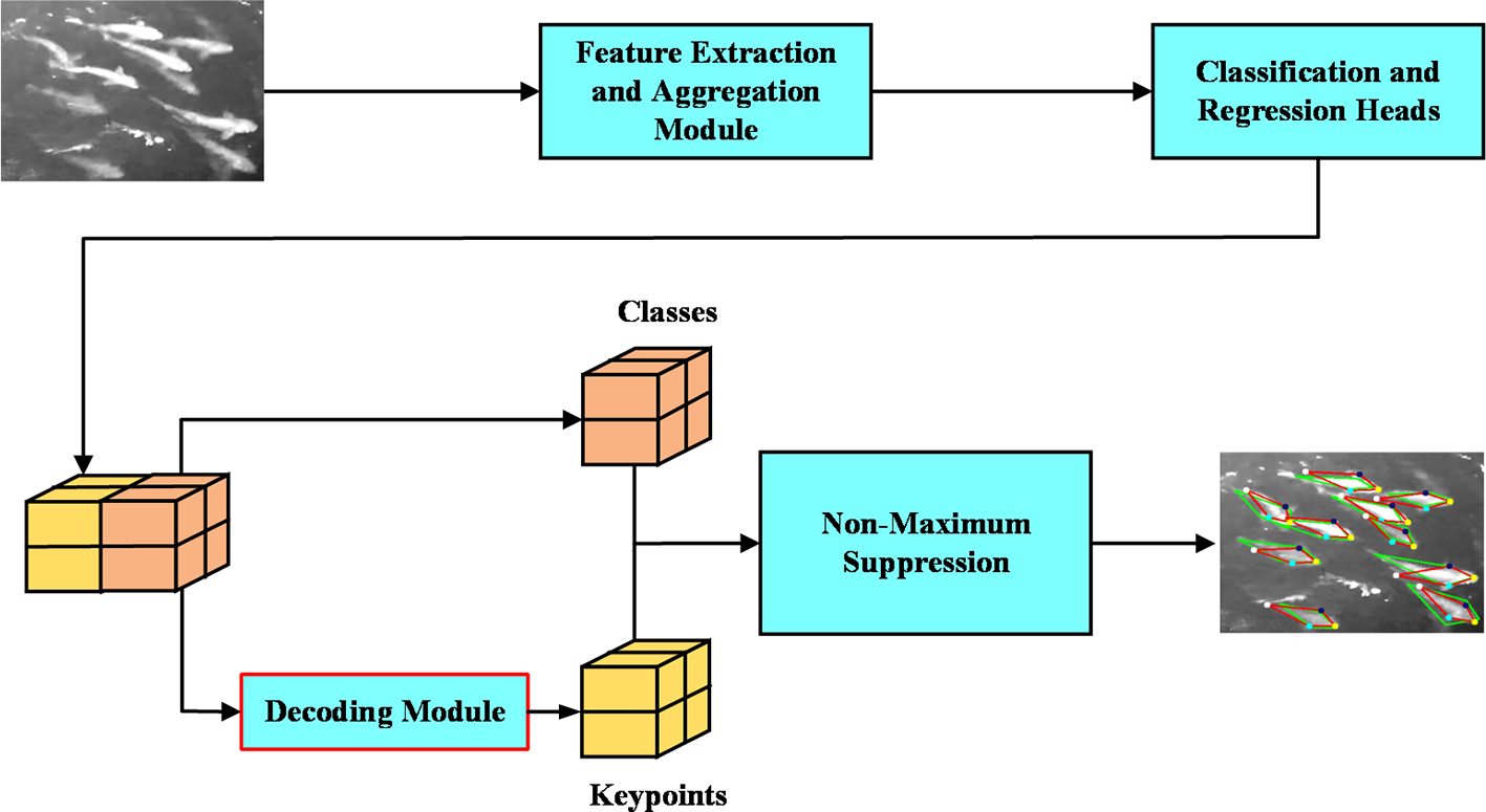
Model architecture for fish keypoints detection. The main difference between this architecture and a typical keypoint regression network lies in the decoding module, which plays a crucial role in ensuring robustness.
2.2 Shape model of fish
Inspired by the Point Distribution Model (PDM) proposed by Cootes and Taylor (1992), we use the principal components and corresponding eigenvalues of fish keypoints, obtained through PCA, to construct a shape model of fish. From a probabilistic perspective, PCA can be viewed as fitting the data to a multi-dimensional Gaussian distribution. In this context, the principal components and eigenvalues correspond to the major axes of the Gaussian ellipse and the variances of the samples’ projections onto these axes. Generally speaking, with a Gaussian representation, we can utilize the Mahalanobis distance to identify outliers, as it measures the distance between a sample and the Gaussian distribution. Similarly, using this PCA-based model, we can determine whether a shape composed of four points is a valid representation of a fish shape.
By performing alignment, the PDM model inherently disregards the translation and rotation of the shape. To address this limitation, we apply data augmentation to the aligned data. The construction of the PCA-based shape model of fish can be summarized in four key steps: (1) Alignment of Fish keypoints, (2) PCA of Aligned keypoints, (3) Data Augmentation via Unscented Transformation, and (4) PCA of Augmented keypoints. The complete workflow is shown in Figure 3 and the method’s detailed introduction is as follows.
Figure 3
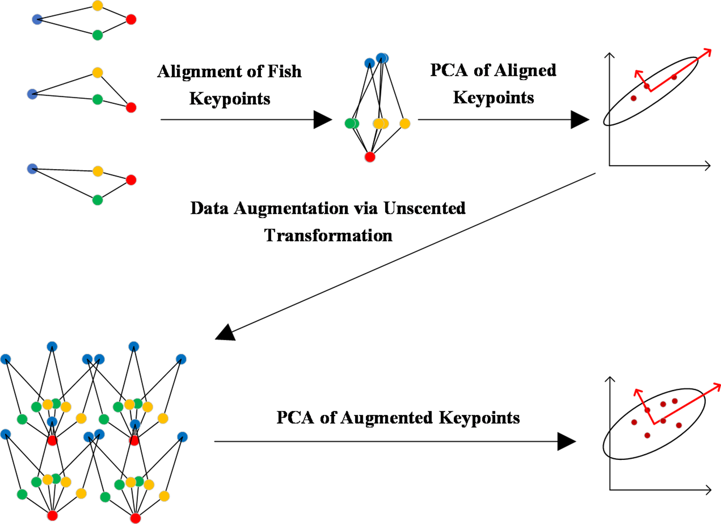
Data flow diagram for building the PCA based shape model of fish. It consists of four steps: (1) Alignment of Fish keypoints, (2) PCA of Aligned keypoints, (3) Data Augmentation via Unscented Transformation, and (4) PCA of Augmented keypoints.
The keypoint vector of the ith fish in the dataset is defined as , where the keypoint indices 1, 2, 3, 4 correspond to the coordinates of the fish head, the left fin, the tail, and the right fin, respectively, within the image coordinate system. Thus, the set of fish keypoints constructed from all individuals in the training set is denoted as , where represents the number of fish samples in the training set. This set, , serves as the input for building the shape model of fish.
-
(1) Alignment of Fish keypoints: The aligned keypoints set is obtained by translating all samples to a common coordinate system, with the fish head at the origin and the fish tail aligned with the y-axis.
-
(2) PCA of Aligned keypoints: This step yields the average shape of fish , the principal component matrix , and the corresponding eigenvalue vector . Specifically, measures the variance of the sample data along the corresponding principal components .
-
(3) Data Augmentation Based on Unscented Transformation: The alignment in step (2) assumes a precise head-to-head match between the anchor fish and ground truth fish, which limits its ability to capture cases where they don’t align perfectly. To overcome this limitation, we can employ data augmentation to generate new samples by introducing translation and rotation perturbations. This can help mitigate the issue, but the large size of the original dataset means that the augmented dataset would be prohibitively large, making PCA computationally costly. Fortunately, since PCA represents the input data as a multidimensional Gaussian distribution, we can apply the unscented transform to obtain a compact set consisting of sigma points. By applying data augmentation to these sigma points, we can significantly reduce the required sample size.
-
Specifically, using the PCA results from step (1), which model a multidimensional Gaussian distribution, the sigma points set can be derived using Equations 1, 2.
-
where represents the dimension of the , and is a tunable parameter that controls the distance of the sigma points from the mean. In this paper, is 8 and is set to 3. Since each sample in has a different weight, it is essential to resample them to ensure that all weights are equalized to 1. Finally, the resampled samples are subjected to rotation and translation perturbations to generate the augmented keypoints . The extent of these perturbations can be controlled by setting different ranges for rotation and translation.
-
(4) PCA of Augmented keypoints: By performing PCA on , the final shape model, represented as , and , can be obtained.
2.3 Anchor fish
Object detection networks often use anchor boxes as prior knowledge of object location and size, allowing the bounding box regression head to learn the deviation between the ground truth and its corresponding anchor box, thereby balancing the loss between large and small objects and improving accuracy. We propose the anchor fish set (Figure 4), which plays a similar role to anchor boxes but is more suitable for fish keypoint regression. The average shape of fish serves as a baseline for generating the anchor fish set. As shown in Figure 4, each grid point in the feature map is associated with a set of 8 anchor fish, consisting of the average shape of fish and multiple fish keypoint vectors generated by rotating the average shape around that point. The anchor fish set , comprising these 8 anchor fish at each grid point in all output feature maps, has two main functionalities: firstly, identifying positive samples during training; secondly, encoding ground truth keypoints during training and decoding the outputs of the regression heads during detection.
Figure 4
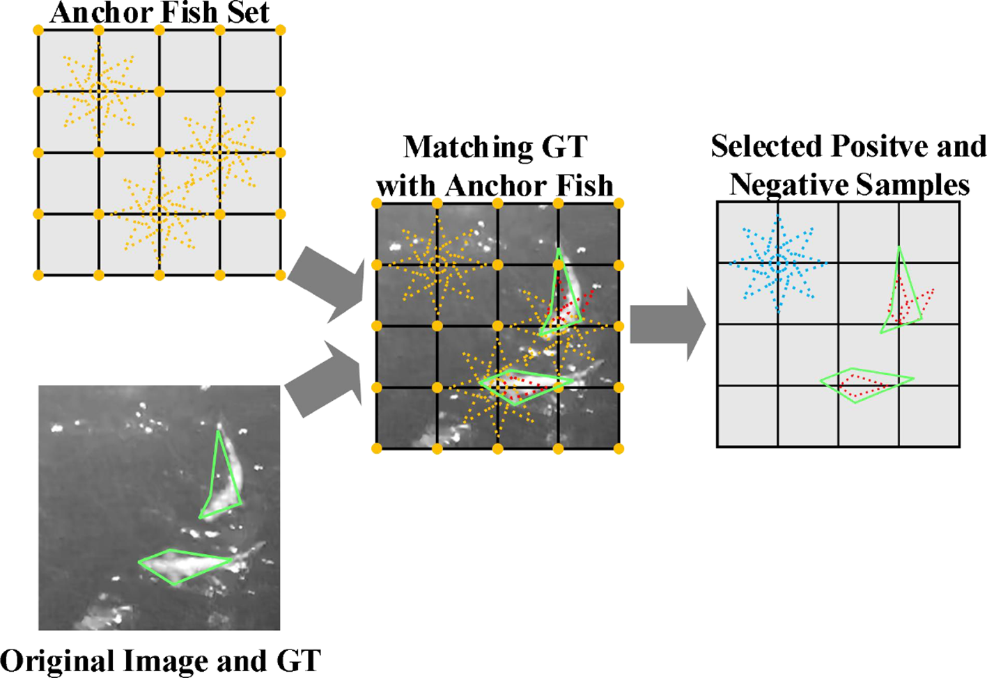
Illustration of anchor fish and positive/negative sample selection process. The yellow dashed fish represents the anchor fish, the green solid fish represents the ground truth fish (GT), and the red dashed fish and blue dashed fish represent the positive and negative samples, respectively, selected from the anchor fish.
A schematic diagram of the anchor fish set and the positive samples selection process (PSS) is shown in Figure 4. Advanced feature extraction networks often employ multi-resolution modules, such as FPN, which generate feature maps at various resolutions. As a result, the inputs to PSS consist of feature maps at different resolutions, their corresponding anchor fish, and the ground truth keypoint vectors represented in the coordinate system of those feature maps. Additionally, PSS requires computing the similarity between each anchor fish in the anchor fish set and every ground truth fish, prompting the definition of a fish-to-fish distance function. By setting a distance threshold, anchor fish with a distance less than the threshold are selected as positive samples for training, while those with a distance greater than the threshold are deemed negative samples. This process completes the selection of positive and negative samples, as well as the matching of positive samples (anchor fish) with ground truth fish, denoted as . Several options exist for fish-to-fish distance, including Euclidean distance and Mahalanobis distance. To minimize computational burden and improve training efficiency, this study adopts the Euclidean distance between two vectors as the fish-to-fish distance function. Once a match is established between a specific anchor fish and a specific ground truth fish, the anchor fish can serve as the average shape for performing principal component-based encoding on its matched ground truth fish, denoted as Equation 3:
where represents the number of the principal components used for encoding. In our application, needs to satisfy the condition .
2.4 Loss function
The shape model introduced in Section 2.2 provides not only the principal directions of the fish keypoints dataset but also the variances associated with these directions. As a result, we can compute the Mahalanobis distance between the regression head output and the shape distribution. This allows us to determine the degree of variation that is reasonable for a typical fish within specific principal directions. By using this distance as a loss score, we can further constrain the output to conform to the fish shape distribution. Accordingly, we propose a loss function consisting of three parts: classification loss, encoded keypoints loss, and shape variation loss,
where , and are hyperparameters that modulate the impact of different loss components on the total loss.
The index set of positive samples is denoted as , having a cardinality of , and the index set of negative samples is denoted as , having a cardinality of . The output of the ith classification head is , where and is the probability of the fish and background respectively. The collection of all classification head outputs forms the set . Then, the classification loss can be computed using the softmax loss, as shown in Equations 5, 6:
Encoded keypoints loss reflects the deviation between the output of the regression head and the encoded ground truth keypoints. To compute this loss, we use smooth L1. Let be the output of the regression head for the ith anchor fish, and let P be the set of all regression head outputs. Then, the classification loss can be computed using thesoftmax loss, as shown in Equation (5) and Equation (6):
Similar to Mahalanobis distance, the shape variation loss is computed as follows:
3 Experimental setup and results
Before conducting experiments, we first established our own fish image dataset using above-water infrared cameras and constructed the PCA-based shape model of fish. The experiments are designed to focus on comparing performance across different network architectures and key hyperparameters. In the comparison experiments, our dataset is split into training, validation, and test sets, comprising 406, 45, and 157 images, respectively. All training processes are run for 500 epochs.
3.1 Establishing dataset
The images of our dataset were derived from continuous 24-hour infrared video footage recorded by cameras (Hikvision DS-2CD6626B-IZHRS, manufactured by Hangzhou Hikvision Digital Technology Co., Ltd in Hangzhou, China) mounted on a truss-structure net cage located in the water off Kuishan Island, Zhuhai, China, as illustrated in Figure 5a. We specifically selected videos recorded during nighttime (8:00 p.m. – 04:00 a.m.) and under moderate wind conditions (4–7 m/s) during June and July, and then randomly sampled image frames from these videos for labeling. We used this selection criterion because it was extremely difficult to distinguish fish in daytime images due to significant camera-to-water-surface distance, turbid seawater condition and intense specular reflections, which severely obscured fish outlines (Figure 5b). Conversely, nighttime images provided significantly enhanced fish visibility necessary for reliable detection (Figure 5c). Furthermore, the selected wind speeds induced greater fish activity within the net cage, providing a more diverse range of fish postures essential for training a model with good generalization.
Figure 5
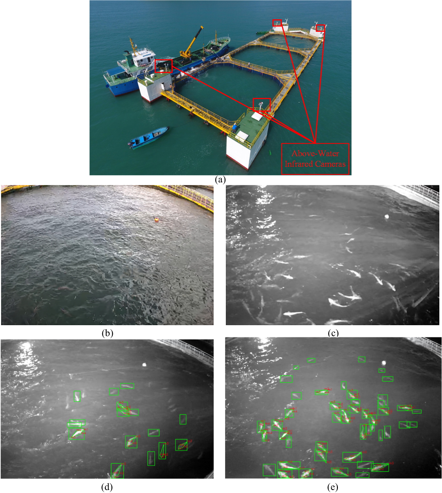
(a) Offshore truss-structure net cage with above-water infrared cameras for fish data collection; (b) Images collected during the day; (c) Images collected at night; (d, e) Labeled images.
The dataset comprises 608 images, and the image size was 3 × 1920 × 1080. The fish keypoints were annotated using Labelme (v5.3.1), an open-source annotation tool. There are a total of 12,516 fish annotated with bounding boxes and 8,066 fish annotated with keypoints. The disparity between the number of bounding boxes and keypoint annotations arises from the fact that some fish keypoints are not clearly visible in the images, and were therefore not annotated. Examples of the labeled dataset are shown in Figures 5d, e.
3.2 Constructing the PCA-based shape model of fish
Figure 6 illustrates the fish shapes generated by individually varying the average shape along each principal component direction, based on formula . The degree of deviation from the average shape of fish along a principal component is represented by k, which takes on 11 uniformly selected values ranging from -3 to 3. Additionally, we present a curve showing the eigenvalues in descending order, as shown in Figure 7.
Figure 6
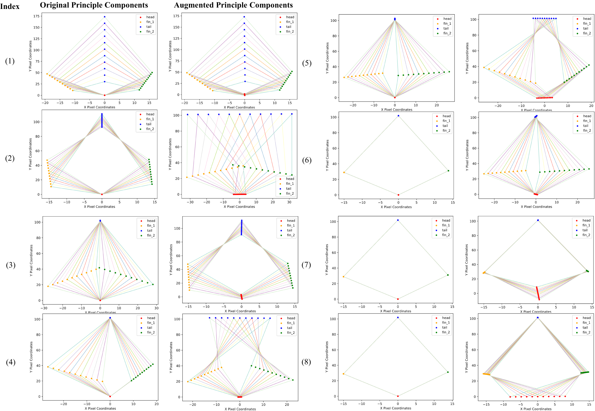
Fish shapes generated by principal components: original (left) vs. augmented (right).
Figure 7
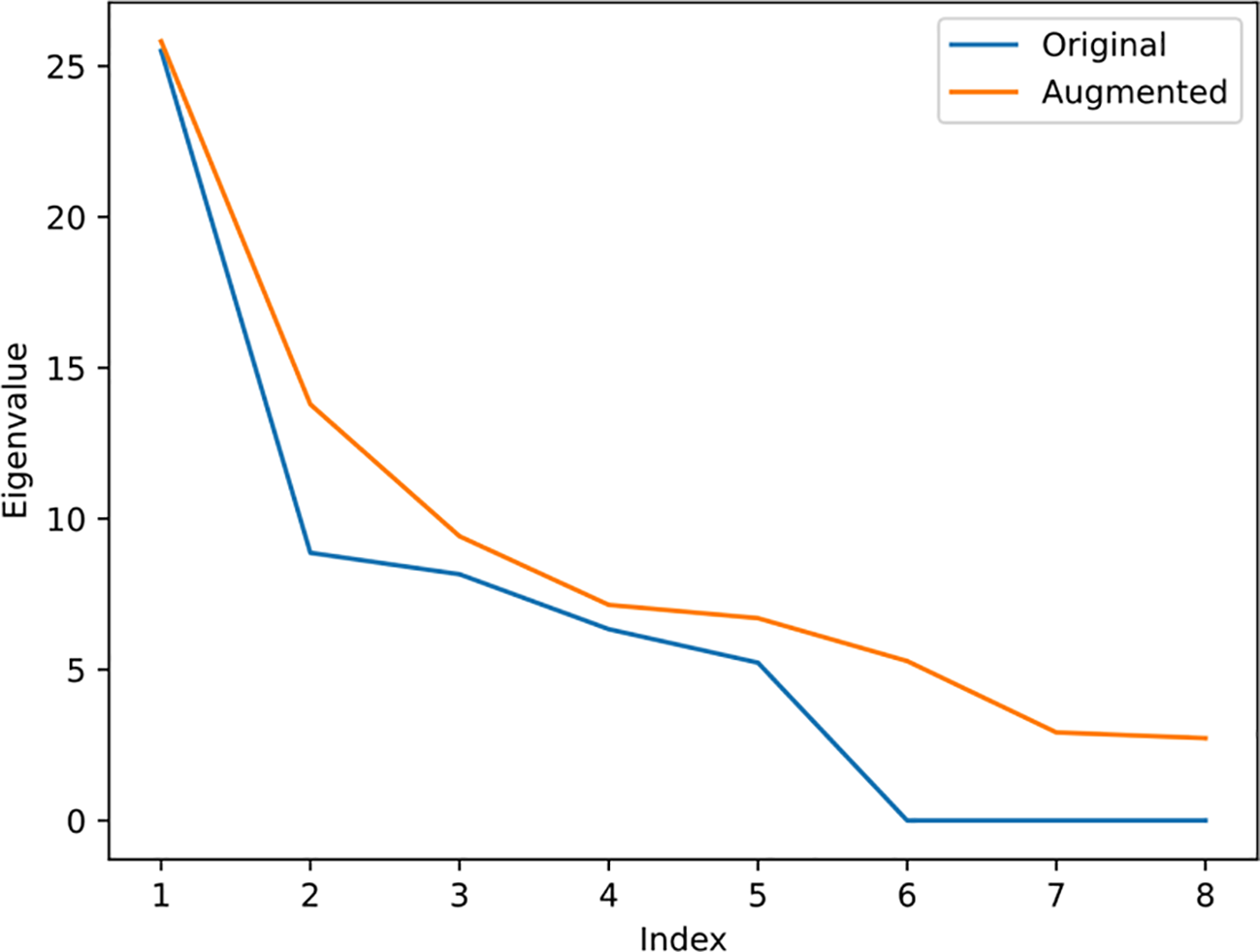
Original and augmented eigenvalues in descending order. The results show that after data augmentation, all eigenvalues have increased.
The fish shapes in the first column of Figure 6 are generated from the original principal components, with all fish heads aligned to the origin and tails extending along the y-axis. These shapes demonstrate that different principal components capture various modes of shape variation. Specifically, the first and second principal components account for changes in fish length and width, while the third to fifth principal components capture shape changes resulting from different swimming poses. In contrast, the shapes generated by the 6th to 8th principal components are nearly identical to the average shape, indicating that these components have a negligible impact on shape variation. This is because the variance of the keypoint training samples projected in these directions is extremely small, close to zero. The second column of Figure 6 displays fish shapes generated by applying unscented transform-based data augmentation to the original PCA results. The perturbations in the x-direction, y-direction, and orientation-direction are set to en pixels, ixe pixels, and ls0nd respectively. The results show that, in addition to modeling size and swimming pose, the principal components also capture the displacement and rotation of a fish. Furthermore, the eigenvalue curve reveals that the eigenvalues associated with the original principal components from index 6 to 8 are near zero, indicating minimal contribution to shape variation. However, after augmentation, all eigenvalues have increased, indicating an increase in the uncertainty of the shape distribution.
3.3 Comparison experiments on different keypoint regression networks
The core idea of our experimental design is to improve a simple keypoint detection network through our encoding method, thereby surpassing the performance of a finely designed network. Consequently, we chose RetinaFace and YOLO5face as baseline models for they are both widely used networks and exhibit significant performance disparity in keypoint detection task. While RetinaFace has a comparatively straightforward network structure, YOLO5Face is a state-of-the-art, highly engineered detector building upon YOLOv5, incorporating advanced modules like a ShuffleNetV2-based backbone, a Stem structure, CSP (Cross Stage Partial) blocks, SPP (Spatial Pyramid Pooling) module, and the wing loss function.
YOLO5Face used in our experiment adopts the YOLOv5s architecture, and all hyperparameters are sourced from the authors’ open-source code, which is available at the following URL: https://github.com/deepcam-cn/yolov5-face. RetinaFace employs VGG16 as its backbone, combined with a FPN and context module as its neck. Given the relatively small size of a fish in the full image, a two-layer FPN structure is used, with downsampling ratios of 8 and 16, respectively. In contrast, our method uses the same backbone and neck as RetinaFace, but incorporates anchor fish, PCA-based keypoint encoding with perturbations of tu pixels, ixe pixels, and ls0nd and a loss function defined by Equation 4 with three loss weights (classification loss, encoded keypoints loss, and shape variation loss) set to 2, 1, and 0.07, respectively. Furthermore, this experiment also evaluates the accuracy of using only anchor fish for classification, without performing keypoint regression. It is worth mentioning that the weights for the classification loss and the encoded keypoints loss are set to 2 and 1, respectively, through empirical tuning. While these values were not exhaustively grid-searched, they ensured stability and convergence throughout the training process. The weight for the shape variation loss is determined through the comparative experiments described in Section 3.4, with the optimal setting being 0.07.
To evaluate the performance of keypoint detection, we adopt the evaluation method mentioned in the widely used COCO dataset (Lin et al., 2014). This method defines the Object Keypoint Similarity (OKS), which is used to calculate the similarity between two sets of input keypoints. Based on OKS, Average Precision (AP) can be further calculated, and its function is similar to the Intersection over Union (IoU). We set the parameter “kpt_oks_sigmas” to [0.06, 0.06, 0.06, 0.06] and configured “maxDets” to 80. Results are presented in Table 1. The results show that our method (fifth row) achieved the best performance on the AP50 metric, with a score of 0.656, significantly outperforming the other three methods. Notably, our method outperforms RetinaFace across all AP metrics without altering the network architecture, solely by employing the three methods proposed in this paper. Additionally, our method surpasses the network with only anchor fish-based classification, validating the necessity of the regression head. However, our method has its limitations. Specifically, the AP75 metric is only 0.064, lower than YOLO5Face’s 0.217. As shown in Figure 8, the keypoints detected by YOLO5Face are closer to the ground truth, but it may output invalid fish shapes (indicated by red boxes) and tend to miss more fish without anchor fish. In contrast, our method outputs valid shapes, but loses information after decoding. This is because the shape model derived from aligned keypoints fails to accurately capture translation and rotation, even after unscented transform-based augmentation, in contrast to coordinate-based regression.
Table 1
| Detection Network | AP50 | AP75 | AP |
|---|---|---|---|
| RetinaFace | 0.431 | 0.028 | 0.126 |
| YOLO5Face | 0.503 | 0.217 | 0.256 |
| RetinaFace + Our method without regression | 0.347 | 0.007 | 0.083 |
| RetinaFace + Our method | 0.656 | 0.064 | 0.231 |
Comparison results of different keypoint regression networks.
The bolded values in the table indicate the best value within each column.
Figure 8
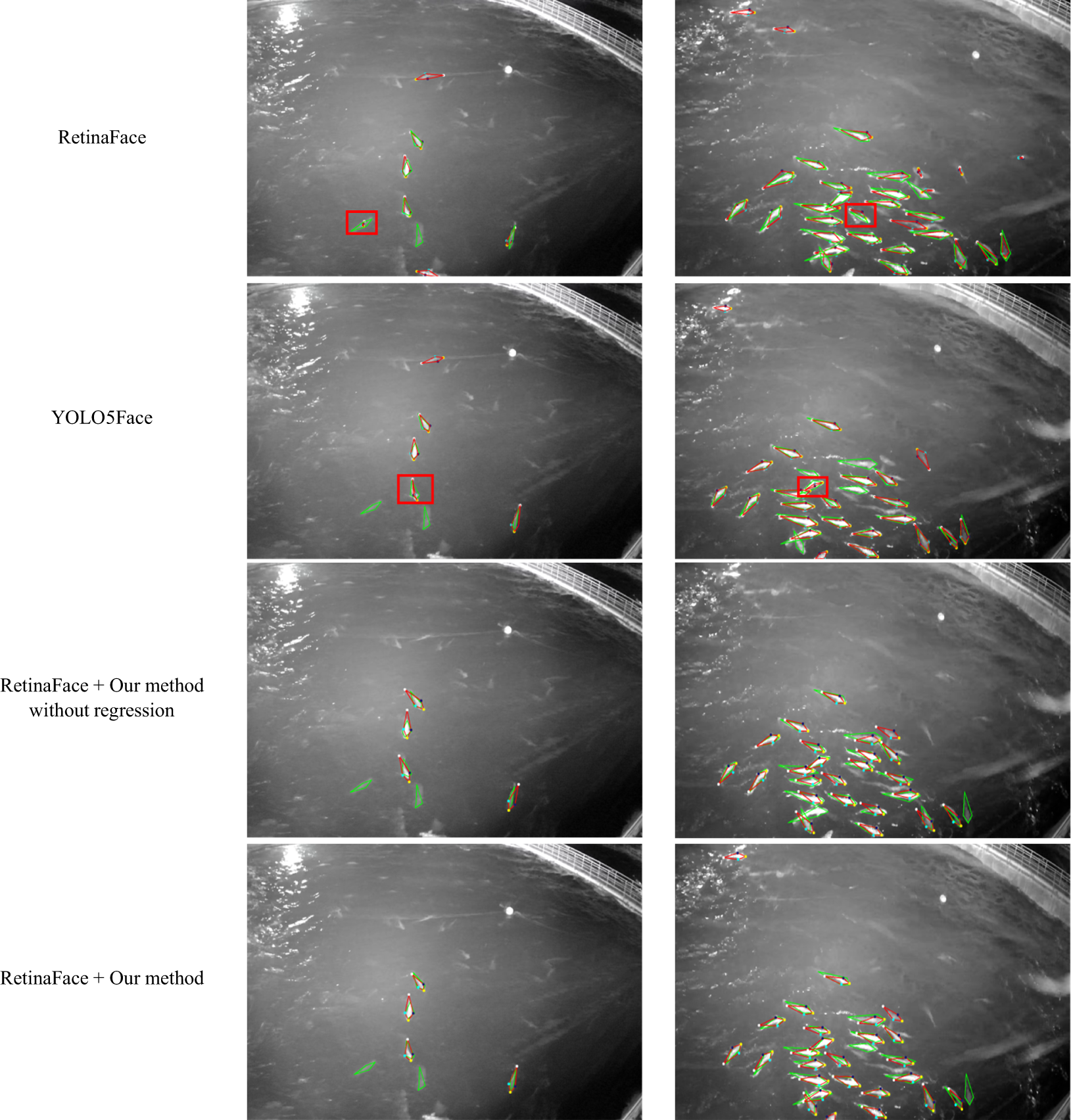
Fish keypoints detection results of different networks. The red fish represent the detection results, and the green fish represent the ground truth. The red boxes highlight the outputs of invalid fish shape. The first row to the fourth row correspond to RetinaFace, YOLO5Face, Improved RetinaFace using our method without regression, and Improved RetinaFace using our method, respectively. The results show that our network consistently outputs valid fish shapes.
3.4 Comparison experiments on different hyperparameters
This experiment examines the effect of varying the number of the selected principal components used for encoding (which influences the size of the output encoded feature vector) and selecting different perturbation parameters for unscented transform on the AP metric. To isolate the impact of shape variation loss, the loss weights for all models are set to 2, 1, and 0. The “PCA_Original” represents a network without unscented transform-based data augmentation. In contrast, the “PCA_a_b_c” networks incorporate data augmentation with perturbation parameters a, b, and c, which correspond to orr pixels, ixe pixels, and nde°n respectively. The results in Table 2 reveal that accuracy increases with the number of the selected principal components. However, larger perturbations in data augmentation do not always yield better results. The optimal accuracy is achieved with the parameter setting of 1_1_2p5.
Table 2
| Perturbation parameters | Number of selected principal components | AP50 | AP75 | AP |
|---|---|---|---|---|
| PCA_Original | 5 | 0.513 | 0.030 | 0.152 |
| PCA_Original | 6 | 0.538 | 0.035 | 0.164 |
| PCA_Original | 7 | 0.554 | 0.057 | 0.172 |
| PCA_Original | 8 | 0.628 | 0.091 | 0.238 |
| PCA_1_1_2p5 | 5 | 0.544 | 0.030 | 0.155 |
| PCA_1_1_2p5 | 6 | 0.549 | 0.044 | 0.170 |
| PCA_1_1_2p5 | 7 | 0.563 | 0.053 | 0.188 |
| PCA_1_1_2p5 | 8 | 0.640 | 0.101 | 0.245 |
| PCA_2p5_2p5_5 | 5 | 0.511 | 0.033 | 0.152 |
| PCA_2p5_2p5_5 | 6 | 0.528 | 0.034 | 0.157 |
| PCA_2p5_2p5_5 | 7 | 0.560 | 0.053 | 0.180 |
| PCA_2p5_2p5_5 | 8 | 0.631 | 0.090 | 0.233 |
| PCA_5_5_10 | 5 | 0.546 | 0.036 | 0.165 |
| PCA_5_5_10 | 6 | 0.557 | 0.040 | 0.171 |
| PCA_5_5_10 | 7 | 0.587 | 0.040 | 0.186 |
| PCA_5_5_10 | 8 | 0.634 | 0.090 | 0.240 |
Comparison results of different perturbation parameters and number of selected principal components.
The bolded values in the table indicate the best value within each column.
Furthermore, we utilize PCA_5_5_10 as the base network and investigate the impact of shape variation loss weight on accuracy. As shown in Table 3; Figure 9, adjusting the weight of the shape variation loss results in noticeable fluctuations in accuracy. However, the overall trend suggests that as the weight increases, the AP50 metric initially improves before subsequently deteriorating. The peak AP50 accuracy of 0.656 is achieved when the weight is set to 0.07, resulting in a 0.22 improvement over the zero-weight baseline. In contrast, the AP75 metric exhibits a pattern of fluctuating decline, and the AP75 accuracy corresponding to the peak AP50 accuracy is notably lower. This may be attributed to the fact that shape variation loss can be viewed as a form of regularization, which enhances the model’s generalization ability by mitigating overfitting to the training set.
Table 3
| Perturbation parameters | Loss weight | AP50 | AP75 | AP |
|---|---|---|---|---|
| pca_5_5_10 | (2,1,0) | 0.634 | 0.090 | 0.240 |
| pca_5_5_10 | (2,1,0.01) | 0.629 | 0.087 | 0.230 |
| pca_5_5_10 | (2,1,0.02) | 0.639 | 0.077 | 0.232 |
| pca_5_5_10 | (2,1,0.03) | 0.631 | 0.080 | 0.229 |
| pca_5_5_10 | (2,1,0.05) | 0.633 | 0.069 | 0.223 |
| pca_5_5_10 | (2,1,0.07) | 0.656 | 0.064 | 0.231 |
| pca_5_5_10 | (2,1,0.09) | 0.652 | 0.070 | 0.223 |
| pca_5_5_10 | (2,1,0.1) | 0.652 | 0.075 | 0.235 |
| pca_5_5_10 | (2,1,0.2) | 0.632 | 0.084 | 0.229 |
| pca_5_5_10 | (2,1,0.3) | 0.628 | 0.089 | 0.232 |
| pca_5_5_10 | (2,1,0.4) | 0.623 | 0.074 | 0.222 |
| pca_5_5_10 | (2,1,0.5) | 0.635 | 0.063 | 0.219 |
| pca_5_5_10 | (2,1,0.7) | 0.632 | 0.074 | 0.221 |
| pca_5_5_10 | (2,1,0.9) | 0.597 | 0.063 | 0.206 |
Comparison results of different loss weights.
The bolded values in the table indicate the best value within each column.
Figure 9
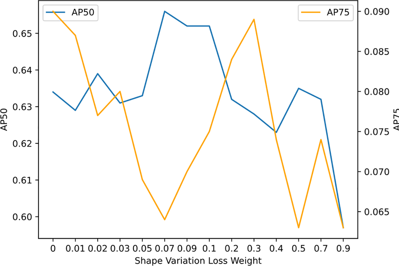
Comparison results of different loss weights. The value of AP50 metric increases first and then decreases, while the value of AP75 shows a “fluctuation-decrease” trend.
3.5 Comparison experiments with outliers
We verified the performance after training the model on a training set with outliers under different shape variation losses. In this experiment, we used three training sets that consisted of 10%, 20%, and 30% outliers, respectively. The outliers were made deliberately by shuffling their keypoint orders, meaning misarranging the order of the head, tail, and fins. Then we set different weights to the shape variation loss and test the model’s performance. The results in Table 4 show that increasing the weight of shape variation loss improves the model’s AP50 performance when the dataset is compromised by outliers, and the higher proportion of outliers exist, the more significant role shape variation loss plays. However, an excessively high weight of shape variation loss can be detrimental to precision. These results demonstrate the robustness of our model to incorrect labels.
Table 4
| Loss weight | 10% outliers | 20% outliers | 30% outliers |
|---|---|---|---|
| (2,1,0) | 0.57 | 0.54 | 0.49 |
| (2,1,0.05) | 0.57 | 0.57 | 0.49 |
| (2,1,0.1) | 0.59 | 0.58 | 0.55 |
| (2,1,0.2) | 0.59 | 0.55 | 0.52 |
Comparison results using training sets that consist of different proportions of outliers.
3.6 Efficiency validation experiment
This experiment verifies the efficiency of the RetinaFace model before and after improvement using our method. The computer we used is equipped with an NVIDIA RTX 3090 GPU (32GB VRAM) and an Intel Core i9-12900K CPU, and the input image size is 3szee900Knt. The key efficiency metrics are summarized below in Table 5.
Table 5
| Metric | RetinaFace | RetinaFace + our method | Relative change |
|---|---|---|---|
| Number of model parameters | 9.59 M | 9.64 M | + 0.05 M |
| GFLOPS | 623.84 | 623.86 | + 0.02 |
| Inference time per image | 0.04 s | 0.04 s | + 0 s |
Comparison of computational efficiency before and after the integration of our method into RetinaFace.
We can see that the integration of our method incurs only a small change in the number of parameters (0.5% increase) and almost negligible change in GFLOPS (0.02 increase). In addition, the inference time before and after improvement is almost the same, at 0.04 seconds per image. These efficiency metrics confirm the practical suitability of our method for real-time aquaculture monitoring systems.
4 Discussion
From the results in Table 1, it can be seen that the AP75 value of YOLO5Face is 0.217, which is significantly higher than the AP75 value of 0.064 for the method proposed in this paper. This seems to indicate that our method involves a sacrifice in high-precision keypoint regression. However, comparing the original RetinaFace and its improved version, it is clear that our method has improved the AP75 metric for RetinaFace from 0.028 to 0.064, more than doubling it, confirming its ability the enhance precision for a simple detection network. The higher AP75 of 0.217 achieved by YOLO5Face is largely due to its superior network architecture (ShuffleNetV2 backbone, CSP blocks, Wing loss, etc.). To improve AP75 while preserving the shape validity, we propose two approaches that we will carry out in our future studies. One approach is to adopt a more advanced network, such as YOLOv5Face. Another method involves setting both the PCA encoding head and the traditional local coordinate regression head in the network and fusing their outputs using a weighted fusion or filtering algorithm. We believed that with further refinements of our method, we could boost the AP75 metric while maintaining high AP50 and shape validity.
The robustness claimed in our work primarily relates to resilience against outliers, similar to the core principle of the RANSAC (Random Sample Consensus) algorithm, which mitigates the influence of outliers during model fitting. Our method similarly exhibits robustness in two critical aspects:
-
(1) Outlier Rejection During Inference: It explicitly constrains the output keypoints to form valid fish shapes, preventing implausible predictions.
-
(2) Outlier Tolerance During Training: It demonstrates resilience against mislabeled training data, reducing their adverse impact on keypoint regression performance.
From the results in Table 3, it can be observed that the shape variation loss introduces a trade-off between the AP50 and AP75 values. This is due to that a high weight assigned to the shape variation loss might lead to an increase in landmark loss during training. Through further analysis, it can be seen that if the labeled fish in the training set fits well with the anchor fish, the shape variation loss will be small enough that the trade-off will not occur, even with a higher weight being assigned to it. When the labeled fish in the training set deviates too far from the anchor fish, shape variation loss will increase and assigning a high weight to it will lead to an increase in encoded keypoint loss during the training process. However, whether this trade-off benefits the model’s performance depends on what causes the labeled fish to deviate from the anchor fish. If the deviated fish have valid fish shapes but are too large or small, or their poses differ from the anchor fish, increasing the weight of the shape variation loss will impair the model’s ability to learn high-precision coordinate regression. On the other hand, if the deviations are caused by incorrectly labeled coordinate values or coordinate order, the larger value of shape variation loss is beneficial, for it will prevent the model from fitting into incorrectly labeled keypoints. An example can be seen from section 3.5.
In the training set, some low-visibility fish have unlabeled keypoints, and thus these keypoints are not learned by the model. We conducted the following validation specifically for low-visibility fish. As we can see in Figure 10, there are 18 and 15 annotated fish (green quadrilaterals) in Figures 10a, b respectively, 12 and 6 low-visible fish (red dots) in Figures 10c, d respectively. Notably, our model detected 27 and 16 fish (red quadrilaterals) as shown in Figures 10c, d respectively. Further analysis of the fish detected by our model, we can see that there are a total of 43 fish detected, which significantly exceeds the 33 annotated ones. Comparison between the annotated fish and detected ones shows that 29 detections correctly correspond to annotated ones, with only 4 missing, and 1 false positive. Comparison between the low-visible fish and detected ones shows that 13 detections correctly correspond to the low-visible ones, with 5 missing, but no false positive.
Figure 10
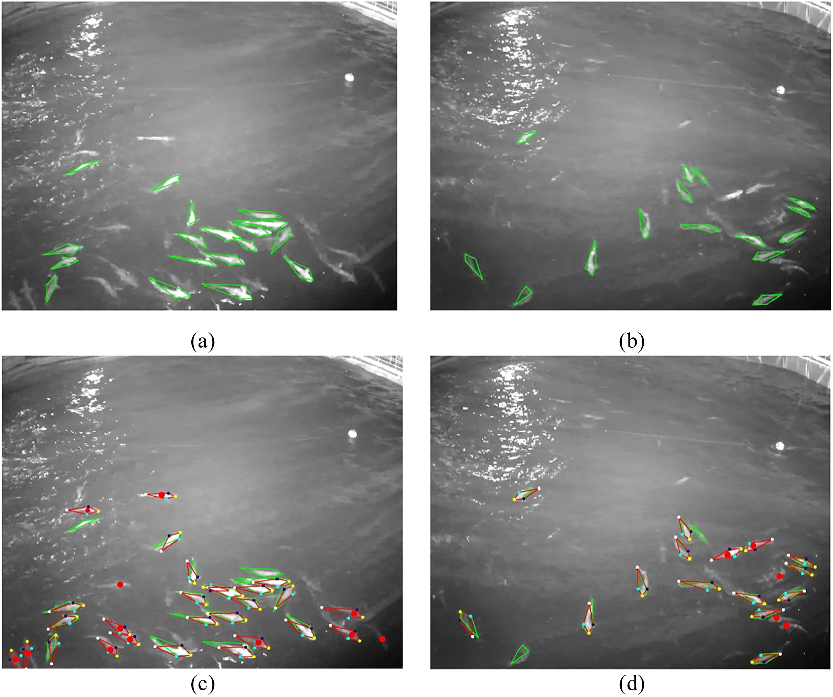
Illustration of the detection results of low-visibility fish. The green quadrilaterals indicate the labeled fish, the red quadrilaterals indicate the detected fish, and the red dots indicate the unlabeled low-visibility fish. (a, b) Images with labeled fish; (c, d) Images with labeled and detected fish.
By analyzing the detection results on the test set, the failure cases can be divided into three categories:
-
(1) Low-visibility fish that are not labeled but detected, which should not be treated as a real failure.
-
(2) Detected fish that are either false positives (FP) or false negatives (FN). Further analysis shows that FP are mainly caused by specular reflections (Figure 11a) or confusion between the fish head and fish tail (Figure 11b), while FN mostly occur when fish is too small or unclear for detection (Figure 11c), or when fish overlap (Figure 11d). In some rare cases, fish with clear outline are still missed, mainly because the anchor fish closest to them is misclassified as background (Figure 11e).
-
(3) Detected fish with significant deviations in keypoints, which are often caused by tail mislocalization (Figure 11f).
Figure 11
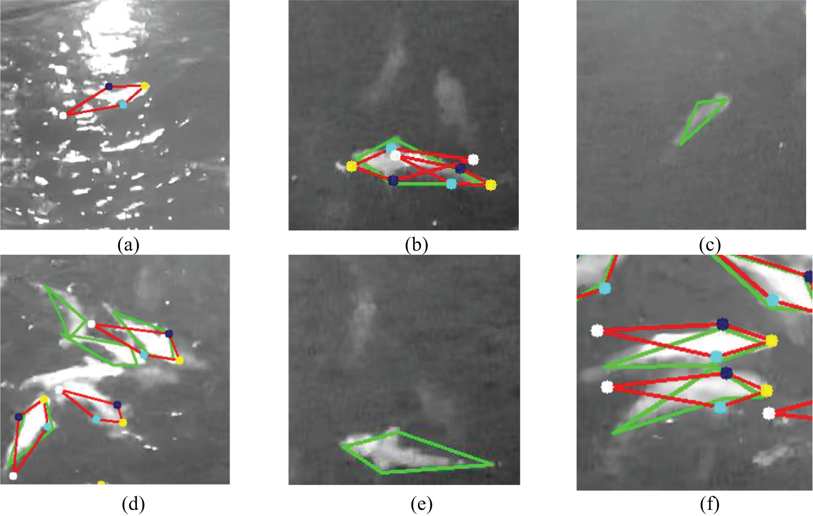
Examples of failure cases of our method. The green quadrilaterals indicate the labeled ground truth fish, the red quadrilaterals indicate the detected fish: (a) FP caused by specular reflection; (b) FP caused by confusing the head and tail; (c) FN caused by small or low-visibility fish; (d) FN caused by overlapping; (e) FN caused by low classification score; (f) Large keypoint error caused by the tail mislocalization.
5 Conclusions
In this paper, we have established a fish keypoint dataset using images captured by above-water infrared cameras and proposed three strategies to improve an existing keypoint detection network RetinaFace. These strategies significantly improve the AP50 score, avoid the generation of invalid fish keypoints, and prevent the model from fitting to outliers in the training set, thus ensuring robustness. This is highly beneficial for subsequent size and quantity estimation as well as behavior analysis tasks in offshore aquaculture. Our approach involves principal component-based shape encoding and a loss function that incorporates shape variation loss to constrain the output of regression heads. Additionally, we utilize anchor fish as a prior for fish objects to improve detection rates. We conducted comparative experiments using a dataset from above-water infrared cameras installed on a truss net cage to validate the effectiveness of our method. The results demonstrate that our method outperforms the well-designed YOLO5Face keypoint detection network in AP50 metrics, with each output keypoint vector constituting a valid fish shape. To further investigate the characteristics of our proposed methods, we conducted comparative experiments on three key hyperparameters and different rate of outliers in the training set. The experimental results elucidate the characteristics of our method and its robustness to incorrect labels. Notably, our method can be used to improve any anchor-based object detection network, especially those with carefully designed architectures, thereby achieving higher AP50 and AP75 values.
Statements
Data availability statement
The datasets presented in this study can be found in online repositories. The names of the repository/repositories and accession number(s) can be found below: https://github.com/LMX-BY/fish_landmark_detection_using_PCA_based_fish_shape_model.
Ethics statement
The manuscript presents research on animals that do not require ethical approval for their study.
Author contributions
GL: Conceptualization, Writing – review & editing, Methodology, Software, Funding acquisition, Writing – original draft. AL: Resources, Methodology, Visualization, Writing – review & editing, Software. ZY: Formal analysis, Data curation, Validation, Writing – review & editing, Software. YH: Investigation, Resources, Writing – review & editing, Validation, Formal analysis, Data curation. GP: Writing – review & editing, Supervision, Formal analysis, Validation, Visualization. TY: Writing – review & editing, Visualization, Supervision, Validation. ZL: Funding acquisition, Supervision, Writing – review & editing, Validation. XH: Conceptualization, Supervision, Funding acquisition, Project administration, Writing – review & editing. GW: Writing – review & editing, Validation, Funding acquisition, Resources.
Funding
The author(s) declare that financial support was received for the research and/or publication of this article. This work was supported in part by the National Natural Science Foundation of China under Grant No. 32403089 and No. 32173024, in part by the Central Public-interest Scientific Institution Basal Research Fund, CAFS (No. 2023TD97), in part by the earmarked fund for CARS-47, and in part by Hainan Province Science and Technology Special Fund, under Grant No. ZDYF2023XDNY066, and in part by the Central Public-interest Scientific Institution Basal Research Fund, South China Sea Fisheries Research Institute, CAFS, (NO.2023RC01 and NO. 2022TS06).
Conflict of interest
The authors declare that the research was conducted in the absence of any commercial or financial relationships that could be construed as a potential conflict of interest.
Generative AI statement
The author(s) declare that no Generative AI was used in the creation of this manuscript.
Publisher’s note
All claims expressed in this article are solely those of the authors and do not necessarily represent those of their affiliated organizations, or those of the publisher, the editors and the reviewers. Any product that may be evaluated in this article, or claim that may be made by its manufacturer, is not guaranteed or endorsed by the publisher.
References
1
Baltrusaitis T. Robinson P. Morency L. P. (2013). “Constrained local neural fields for robust facial landmark detection in the wild,” in Proceedings of the IEEE international conference on computer vision workshops. (Sydney, NSW, Australia: IEEE). doi: 10.1109/ICCVW.2013.54
2
Cao X. Wei Y. Wen F. Sun J. (2014). “Face alignment by explicit shape regression,” in 2012 IEEE Conference on Computer Vision and Pattern Recognition, (Providence, RI, USA: IEEE) vol. 107, 177–190. doi: 10.1109/CVPR.2012.6248015
3
Cheng B. Xiao B. Wang J. Shi H. Huang T. S. Zhang L. (2020). “Higherhrnet: Scale-aware representation learning for bottom-up human pose estimation,” in Proceedings of the IEEE/CVF conference on computer vision and pattern recognition. (IEEE). doi: 10.1109/CVPR42600.2020.00543
4
Cootes T. F. Taylor C. J. (1992). “Active shape models-’smart snakes’,” in BMVC92: Proceedings of the British Machine Vision Conference. (London, UK: Springer). doi: 10.1007/978-1-4471-3201-1_28
5
Deng J. Guo J. Ververas E. Kotsia I. Zafeiriou S. (2019). “Retinaface: Single-stage dense face localisation in the wild,” in 2020 IEEE/CVF Conference on Computer Vision and Pattern Recognition (CVPR), Seattle, WA, USA, pp. 5202–5211. doi: 10.1109/CVPR42600.2020.00525
6
Dong J. Shangguan X. Zhou K. Gan Y. Fan H. Chen L. (2023). A detection-regression based framework for fish keypoints detection. Intell. Mar. Technol. Syst.1, 9. doi: 10.1007/s44295-023-00002-3
7
Feng Z. H. Kittler J. Awais M. Huber P. Wu X. J. (2018). “Wing loss for robust facial landmark localisation with convolutional neural networks,” in Proceedings of the IEEE conference on computer vision and pattern recognition (Salt Lake City, UT, USA: IEEE). doi: 10.48550/arXiv.1711.06753
8
Han F. Zhu J. Liu B. Zhang B. Xie F. (2020). Fish shoals behavior detection based on convolutional neural network and spatiotemporal information. IEEE Access.8, 126907–126926. doi: 10.1109/ACCESS.2020.3008698
9
He K. Gkioxari G. Dollár P. Girshick R. (2017). “Mask r-cnn,” in Proceedings of the IEEE international conference on computer vision. (Venice, Italy: IEEE). doi: 10.1109/ICCV.2017.322
10
Kazemi V. Sullivan J. (2014). “One millisecond face alignment with an ensemble of regression trees,” in Proceedings of the IEEE conference on computer vision and pattern recognition. (Columbus, OH, USA: IEEE). doi: 10.1109/CVPR.2014.241
11
Kumar N. Biagio C. D. Dellacqua Z. Raman R. Martini A. Boglione C. et al . (2022). “Empirical Evaluation of deep learning approaches for landmark detection in fish bioimages,” in European Conference on Computer Vision (Tel Aviv, Israel: Springer). doi: 10.1007/978-3-031-25069-9_31
12
Labao A. B. Naval P. C. Jr. (2019). Cascaded deep network systems with linked ensemble components for underwater fish detection in the wild. Ecol. Inform.52, 103–121. doi: 10.1016/j.ecoinf.2019.05.004
13
Li W. Li F. Li Z. (2022). Cmftnet: Multiple fish tracking based on counterpoised Jointnet. Comput. Electron. Agric.198, 107018. doi: 10.1016/j.compag.2022.107018
14
Li J. Su W. Wang Z. (2020). “Simple pose: Rethinking and improving a bottom-up approach for multi-person pose estimation,” in Proceedings of the AAAI conference on artificial intelligence (New York, USA: AAAI). doi: 10.48550/arXiv.1911.10529
15
Li W. Wang Z. Yin B. Peng Q. Du Y. Xiao T. et al . (2019). Rethinking on multi-stage networks for human pose estimation (Arxiv). doi: 10.48550/arXiv.1901.00148
16
Li G. Yao Z. Hu Y. Lian A. Yuan T. Pang G. et al . (2024). Deep learning-based fish detection using above-water infrared camera for deep-sea aquaculture: A comparison study. Sensors24, 2430. doi: 10.3390/s24082430
17
Lin T.-Y. Maire M. Belongie S. Hays J. Perona P. Ramanan D. et al . (2014). “Microsoft coco: Common objects in context,” in Proceedings of the European Conference on Computer Vision (ECCV) (Zurich, Switzerland: Springer). doi: 10.1007/978-3-319-10602-1_48
18
Newell A. Huang Z. Deng J. (2017). Associative embedding: End-to-end learning for joint detection and grouping. Adv. Neural Inf. Process. Syst.30. doi: 10.48550/arXiv.1611.05424
19
Newell A. Yang K. Deng J. (2016). “Stacked hourglass networks for human pose estimation,” in Computer Vision – ECCV 2016. ECCV 2016. Eds. LeibeB.MatasJ.SebeN.WellingM. (Amsterdam, The Netherlands: Springer). doi: 10.1007/978-3-319-46484-8_29
20
Qi D. Tan W. Yao Q. Liu J. (2022). “Yolo5face: Why reinventing a face detector,” in European Conference on Computer Vision (Tel Aviv, Israel: Springer). doi: 10.1007/978-3-031-25072-9_15
21
Ramakrishna V. Munoz D. Hebert M. Andrew Bagnell J. Sheikh Y. (2014). “Pose machines: articulated pose estimation via inference machines,” in Computer Vision - ECCV 2014. ECCV 2014. Lecture Notes in Computer Science, vol. 8690 . Eds. FleetD.PajdlaT.SchieleB.TuytelaarsT. (Springer, Cham). doi: 10.1007/978-3-319-10605-2_3
22
Reyes R. del Norte-Campos A. Añasco N. C. Santander-de Leon S. M. S. (2020). Biofouling development in marine fish farm influenced by net colour, immersion period and environmental conditions. Aquacult. Res.51, 3129–3138. doi: 10.1111/are.14648
23
Salama A. J. Satheesh S. Balqadi A. A. (2018). Development of biofouling communities on nylon net panels submerged in the central Red Sea: effects of season and depth. Thalassas.: Int. J. Mar. Sci.34, 199–208. doi: 10.1007/s41208-017-0052-z
24
Saleh A. Jones D. Jerry D. Azghadi M. R. (2023). Mfld-net: a lightweight deep learning network for fish morphometry using landmark detection. Aquat. Ecol.57, 913–931. doi: 10.1007/s10452-023-10044-8
25
Salman A. Siddiqui S. A. Shafait F. Mian A. Shortis M. R. Khurshid K. et al . (2020). Automatic fish detection in underwater videos by a deep neural network-based hybrid motion learning system. ICES. J. Mar. Sci.77, 1295–1307. doi: 10.1093/icesjms/fsz025
26
Saragih J. M. Lucey S. Cohn J. F. (2011). Deformable model fitting by regularized landmark mean-shift. Int. J. Comput. Vis.91, 200–215. doi: 10.1007/s11263-010-0380-4
27
Sun K. Xiao B. Liu D. Wang J. (2019). “Deep high-resolution representation learning for human pose estimation,” in Proceedings of the IEEE/CVF conference on computer vision and pattern recognition. (Long Beach, CA, USA: IEEE). doi: 10.1109/CVPR.2019.00584
28
Suo F. Huang K. Ling G. Li Y. Xiang J. (2020). “Fish keypoints detection for ecology monitoring based on underwater visual intelligence,” in 2020 16th International Conference on Control, Automation, Robotics and Vision (ICARCV). (Shenzhen, China: IEEE). doi: 10.1109/ICARCV50220.2020.9305424
29
Wei S. E. Ramakrishna V. Kanade T. Sheikh Y. (2016). “Convolutional pose machines,” in Proceedings of the IEEE conference on Computer Vision and Pattern Recognition (Las Vegas, NV, USA: IEEE). doi: 10.48550/arXiv.1602.00134
30
Wu R. Deussen O. Li L. (2022). “Deepshapekit: accurate 4d shape reconstruction of swimming fish,” in 2022 IEEE/RSJ International Conference on Intelligent Robots and Systems (IROS). (Kyoto, Japan: IEEE). doi: 10.1109/IROS47612.2022.9982097
31
Xiao B. Wu H. Wei Y. (2018). “Simple baselines for human pose estimation and tracking,” in Proceedings of the European Conference on Computer Vision (ECCV) (Munich, Germany: Springer), 466–481. doi: 10.48550/arXiv.1804.06208
32
Yang L. Liu Y. Yu H. Fang X. Song L. Li D. et al . (2021). Computer vision models in intelligent aquaculture with emphasis on fish detection and behavior analysis: a review. ACM Trans. Comput. Eng.28, 2785–2816. doi: 10.1007/s11831-020-09486-2
33
Yashunin D. Baydasov T. Vlasov R. (2020). MaskFace: multi-task face and landmark detector. arxiv preprint (Arxiv). doi: 10.48550/arXiv.2005.09412
34
Yu Y. Zhang H. Yuan F. (2023). Key point detection method for fish size measurement based on deep learning. IET. Image. Process.17, 4142–4158. doi: 10.1049/ipr2.12924
35
Zhao S. Zhang S. Liu J. Wang H. Zhu J. Li D. et al . (2021). Application of machine learning in intelligent fish aquaculture: A review. Aquaculture540, 736724. doi: 10.1016/j.aquaculture.2021.736724
36
Zhong F. Li M. Zhang K. Hu J. Liu L. (2021). Dspnet: A low computational-cost network for human pose estimation. Neurocomputing423, 327–335. doi: 10.1016/j.neucom.2020.11.003
37
Zou Z. Chen K. Shi Z. Guo Y. Ye J. (2023). Object detection in 20 years: A survey. Proc. IEEE.111, 257–276. doi: 10.1109/JPROC.2023.3238524
Summary
Keywords
offshore aquaculture, fish keypoint detection, deep learning, shape encoding, principal component analysis
Citation
Li G, Lian A, Yao Z, Hu Y, Pang G, Yuan T, Li Z, Huang X and Wang G (2025) Fish keypoint detection for offshore aquaculture: a robust deep learning approach with PCA-based shape constraint. Front. Mar. Sci. 12:1619457. doi: 10.3389/fmars.2025.1619457
Received
28 April 2025
Accepted
16 June 2025
Published
07 July 2025
Volume
12 - 2025
Edited by
Marcel Martinez-Porchas, National Council of Science and Technology (CONACYT), Mexico
Reviewed by
Suja Cherukullapurath Mana, PES University, India
Charlie Marzan, Don Mariano Marcos Memorial State University, Philippines
Updates
Copyright
© 2025 Li, Lian, Yao, Hu, Pang, Yuan, Li, Huang and Wang.
This is an open-access article distributed under the terms of the Creative Commons Attribution License (CC BY). The use, distribution or reproduction in other forums is permitted, provided the original author(s) and the copyright owner(s) are credited and that the original publication in this journal is cited, in accordance with accepted academic practice. No use, distribution or reproduction is permitted which does not comply with these terms.
*Correspondence: Xiaohua Huang, huangxhua@scsfri.ac.cn
Disclaimer
All claims expressed in this article are solely those of the authors and do not necessarily represent those of their affiliated organizations, or those of the publisher, the editors and the reviewers. Any product that may be evaluated in this article or claim that may be made by its manufacturer is not guaranteed or endorsed by the publisher.