Abstract
Introduction:
Mangrove ecosystems are increasingly recognised as essential nature-based solutions for enhancing coastal resilience against sea-level rise and climate-induced extreme events. However, achieving robust uncertainty quantification for hydro-morphodynamic models of mangrove systems remains a critical challenge due to the complexity of physical processes and the high computational cost of solving Navier–Stokes partial differential equations. Conventional uncertainty quantification approaches, including Gaussian Process surrogates and physics-informed neural networks, are limited by their inability to adequately capture non-Gaussian behaviour, high-dimensional interactions, or to scale efficiently to large-scale coastal systems.
Methods:
To address these limitations, we propose an efficient and scalable probabilistic framework based on Deep Gaussian Processes, which hierarchically stack multiple Gaussian Process layers to represent complex, multi-scale, and non-Gaussian dependencies in hydro-morphodynamic dynamics. The framework is applied to a high-resolution numerical model of mangrove systems and trained using a variational inference approach to enable efficient surrogate modelling and uncertainty propagation.
Results:
The proposed Deep Gaussian Process model reduces computational cost by more than three orders of magnitude (approximately 1.4 minutes compared to over five days for the full numerical solver), while achieving substantially improved predictive accuracy relative to standard Gaussian Process models. Specifically, a fivefold reduction in error is observed, with an RMSE of 0.0095 m compared to 0.0465 m for conventional Gaussian Processes. The framework enables reliable propagation of uncertainty across complex, nonlinear system dynamics.
Discussion:
These results demonstrate the potential of Deep Gaussian Processes to provide accurate and computationally efficient uncertainty quantification for hydro-morphodynamic modelling of mangrove ecosystems. The proposed approach supports evidence-based planning for climate adaptation and ecosystem-based coastal resilience, offering a practical pathway for integrating advanced uncertainty quantification into operational decision-making for sustainable coastal management.
1 Introduction
Hydro-morphodynamic systems describe the interactions between fluid flow, sediment transport, and morphological evolution across varying spatial and temporal scales (Haun and Dietrich, 2021; Korpak et al., 2023). Governed by conservation laws of mass and momentum (Dey, 2014), these systems play a pivotal role in shaping coastal landscapes, including estuaries and shorelines (Franzen et al., 2021). Within this context, mangrove ecosystems provide a dynamic illustration of hydro-morphodynamic feedbacks. Their root networks attenuate flow velocities, promote sediment deposition, and stabilise shorelines (Mazda et al., 2005). This natural interaction offers ecological resilience while simultaneously exposing mangroves to vulnerabilities associated with sea level rise and anthropogenic disturbances (Gilman et al., 2008). Accurately modeling these processes requires integrated hydrodynamic, sediment transport, and ecological representations, often demanding the use of complex numerical models.
Hydro-morphodynamic modeling has therefore become increasingly central to the design and evaluation of mangrove-based protection strategies against climate-induced sea level rise (Fanous et al., 2023c; Chang and Mori, 2021; Kato and Tajima, 2023).
Nonetheless, significant uncertainties arise due to incomplete knowledge of physical parameters, boundary conditions, and model approximations (Clare et al., 2022). To improve predictive reliability and support resilient coastal management, these uncertainties must be systematically addressed using uncertainty quantification (UQ) techniques. Yet, comprehensive UQ efforts typically demand large ensembles of model simulations, which are computationally prohibitive, particularly in high-resolution or near-real-time scenarios critical for climate adaptation.
Classical UQ methods such as Monte Carlo (MC) sampling, sparse grid approximations, and surrogate modeling are widely used to tackle this issue. Despite their extensive adoption, MC-based UQ becomes impractical when applied to complex high-dimensional hydro-morphodynamic models (Villaret et al., 2016). Even advanced sampling methods like Latin hypercube sampling (Iman and Conover, 1980) and multilevel MC (Giles, 2008) cannot fully overcome these challenges, as exemplified by the 240,000 simulations required in (Harris et al., 2018) for the XBeach model.
To reduce computational costs, surrogate modeling approaches including Polynomial Chaos (PC) expansions, physics-informed neural networks (PINNs), and Gaussian process (GP) emulators have therefore been explored (Li et al., 2021; Raissi et al., 2019; Donnelly et al., 2022, 2024b, a; Fanous et al., 2025). Among these, PC expansions offer an analytical representation of uncertainty propagation by approximating model outputs as polynomials of uncertain inputs, and are efficient for moderate-dimensional and smooth systems. However, they struggle with the curse of dimensionality and fail to capture sharp gradients often observed in nonlinear coastal processes (Wan and Karniadakis, 2005). While stochastic hydro-sediment morphodynamic models based on gPC solvers (Li et al., 2021) have been developed, they largely remain confined to simplified one-dimensional flows. Alternatively, PINNs embed physical laws directly into neural network training, enabling physically consistent learning, but their Bayesian forms (BPINNs) face significant computational bottlenecks due to the size of the parameter space and posterior sampling requirements (Yang and Foster, 2022; Fanous et al., 2023a, b).
Alternatively, PINNs have emerged as powerful tools that embed physical laws directly into neural network training by penalizing deviations from governing equations. This enables them to learn physically consistent solutions while leveraging data-driven flexibility. Bayesian extensions (BPINNs) (Yang and Foster, 2022) further enhance these models by introducing probabilistic priors, allowing for uncertainty estimation and offering improved explainability through posterior distributions over model parameters and outputs. This makes BPINNs particularly attractive for scientific and decision-critical applications, such as coastal protection, where understanding model confidence and variability is crucial. Nevertheless, BPINNs face major scalability bottlenecks in large-scale hydro-morphodynamic models due to the substantial parameter space and computational costs associated with posterior inference. Their training requires extensive optimisation and sampling, making them computationally burdensome, especially when real-time or high-resolution forecasting is needed (Fanous et al., 2023a, b). As such, although BPINNs provide valuable capabilities in terms of explainability and uncertainty quantification, their scalability limitations in complex, high-dimensional environments motivate the exploration of more tractable probabilistic surrogate models.
GP-based emulators remain among the most robust tools for UQ, providing interpretable probabilistic frameworks that naturally quantify predictive uncertainties (Oakley and O’Hagan, 2004; Daneshkhah and Bedford, 2013; Daneshkhah et al., 2017; Batsch et al., 2019). Nevertheless, classical GPs struggle with scalability in high-dimensional output spaces, often requiring dimensionality reduction (DR) techniques (Kennedy and O’Hagan, 2001). Linear DR methods such as Principal Component Analysis (PCA) and non-linear techniques like isometric mapping or Kernel PCA have been employed. However, their deterministic nature and limited ability to capture uncertainty propagation make them suboptimal for complex PDE-based surrogate modeling. Recent coastal studies have further reinforced this limitation. For example, Hossain et al (Hossain et al., 2022). applied empirical and geospatial modeling approaches, such as the Coastal Vulnerability Index, AHP models, and satellite-based shoreline trend analysis, to evaluate risk exposure along the Indian coastline. While valuable, these approaches do not explicitly incorporate probabilistic uncertainty propagation, which limits their application in high-dimensional UQ contexts.
To overcome these limitations, this study explores the Bayesian Gaussian Process Latent Variable Model (BGPLVM) (Titsias and Lawrence, 2010) as a probabilistic DR approach. By mapping high-dimensional outputs onto a lower-dimensional latent space, BGPLVM maintains uncertainty treatment while enhancing computational efficiency. Although previous studies have applied BGPLVM to elliptic PDE surrogates (Atkinson and Zabaras, 2019), its potential remains underexplored in coastal hydro-morphodynamic contexts. BGPLVM offers particular advantages in capturing spatial correlations and facilitating efficient sampling within complex model structures. Other recent studies have introduced hybrid approaches that combine machine learning, geospatial data, and risk modeling, such as the InVEST-CFRM model applied to the Sundarbans (Mondal et al., 2025). While these methods offer valuable insights into flood risk and habitat vulnerability, they typically lack hierarchical probabilistic structures necessary for deep uncertainty propagation.
Despite these developments, achieving efficient and scalable UQ for hydro-morphodynamic systems remains challenging. MC sampling scales poorly with model complexity, and PC expansions suffer from exponential growth in polynomial terms as dimensionality increases. PINNs and their Bayesian variants (BPINNs), although physically consistent, require costly gradient evaluations and posterior sampling, limiting their scalability to large coastal domains. Standard GP surrogates, while fully probabilistic, assume smooth and stationary mappings that cannot represent the strongly non-Gaussian, spatially correlated dynamics typical of coastal morphodynamics. These challenges motivate the exploration of more tractable probabilistic surrogate models such as Deep GPs.
Even so, shallow GP models, even when combined with dimensionality reduction, may still struggle to capture highly non-linear behaviours and non-Gaussian dynamics typical of hydro-morphodynamic systems. Therefore, this paper proposes an advanced framework based on Deep Gaussian Processes (Deep GPs) (Damianou, 2015), which hierarchically stack multiple GPs to model complex, multi-level feature representations. This deep architecture provides more flexibility to model uncertainty across irregular spatial domains and strongly non-linear dynamical processes.
Our investigation leverages simulation data from a detailed numerical model of mangrove hydro-morphodynamics (Fanous et al., 2023a) to compare the performance of traditional single-layer GPs and the proposed Deep GP framework. We systematically evaluate their capabilities in modeling accuracy, uncertainty quantification, computational efficiency, and generalisability across complex domain boundaries. Through this comparative analysis, we aim to advance UQ methodologies for hydro-morphodynamic systems, offering direct relevance to sustainable, nature-based approaches for coastal resilience. Motivated by the above limitations, this study directly addresses a critical research gap by integrating scalable probabilistic machine learning with physically grounded coastal modeling, an approach particularly suited for high-risk, dynamic coastal ecosystems such as the Sundarbans.
Building on the identified research gap, this study sets out the following objectives to guide the analysis and structure of the paper:
-
1. To develop a scalable Deep GP framework for emulating high-dimensional hydro-morphodynamic outputs;
-
2. To perform uncertainty quantification using a variational inference-based sampling approach; and
-
3. To evaluate the performance of the Deep GP model relative to standard GP and full numerical simulation baselines, with a specific focus on mangrove-driven coastal systems.
The paper is structured as follows: Section 2 introduces the governing Navier–Stokes equations and presents the GP-based surrogate modeling approach. Section 3 describes the Deep GP methodology for learning and predicting high-dimensional outputs. Section 4 explains how the trained Deep GP model supports UQ and statistical quantity estimation. Section 5 illustrates the application of the methodology to a mangrove hydro-morphodynamic model. Finally, Section 6 summarises key contributions, study limitations, and future research pathways.
2 Gaussian process-based surrogate modeling for mangrove hydro-morphodynamics
This section presents the application of Gaussian Process (GP) emulators to model the hydro-morphodynamic behaviour of mangrove ecosystems, addressing the challenges posed by the system’s high complexity and nonlinear dynamics. We first outline the governing equations of the hydro-morphodynamic system, to provide the necessary contextual background and to define the regression problem formulated in this work.
Hydro-morphodynamic processes are typically described by the Navier–Stokes (NS) equations for fluid flow, which include both continuity and momentum conservation laws (Fanous et al., 2023c). In coastal regions, where water depth is much smaller than horizontal length scales, the NS equations can be depth averaged, yielding the Shallow Water Equations (SWEs) and substantially reducing computational demands. The 2D depth-averaged SWEs are given as:
where denotes the free surface elevation, represents the depth-averaged velocity vector in the x and y directions, respectively, v is the turbulent kinematic eddy viscosity, g is the gravitational acceleration, and denotes the local water depth relative to the bed elevation .
Equation 1 represents mass conservation, expressing the balance between temporal changes in surface elevation and horizontal divergence of flow. Equation 2 describes momentum conservation, which accounts for advection, diffusion due to turbulence, and pressure gradients induced by surface elevation variations.
Morphodynamic evolution, including sediment transport, is governed by the advection–diffusion equation for depth-averaged sediment concentration :
where is the sediment turbulent diffusivity, given by , with the horizontal viscosity and the turbulent Schmidt number. This equation represents the balance between sediment advection by flow and turbulent diffusion of sediment concentration.
The numerical model incorporating these equations was comprehensively developed and validated in (Fanous et al., 2023a), showing excellent agreement with the tidal gauge data, demonstrating sediment retention properties of mangroves, and highlighting the significant computational expense, with simulations requiring more than five days for 24-hour periods. As sediment dynamics are found to be minimal in the region, this study focuses specifically on modeling water surface elevation as the quantity of interest.
Given the prohibitive computational demands, we aimed to develop a surrogate model, approximating the input–output mapping , where denotes the input variables and the output responses. The surrogate allows rapid estimation of physical quantities such as surface elevation and flow velocities, facilitating efficient uncertainty quantification (UQ).
Following a Bayesian modeling approach (Oakley and O’hagan, 2002), we place a Gaussian Process (GP) prior over the unknown function . Under the GP prior, the finite collection of function evaluations at training inputs follows a joint multivariate normal distribution:
where is the covariance matrix generated by a kernel function. A commonly used kernel is the exponentiated quadratic (RBF) kernel:
where B is a diagonal matrix of positive inverse-squared lengthscales, controlling the correlation decay across input dimensions.
To model noisy observations, we assume additive Gaussian noise:
where denotes the noise variance.
Given training data , the predictive posterior for a new input is also Gaussian:
where the predictive mean and covariance are:
Further details on the derivation of the GP predictive distribution are provided in Supplementary Material, Section 2 (Equations S1–S8).
In sum, the developed GP surrogate provides a powerful probabilistic framework to model and predict hydro-morphodynamic variables efficiently, enabling practical UQ applications in the context of nature based coastal resilience strategies.
3 Enhancing hydro-morphodynamic modeling with deep Gaussian processes
Standard Gaussian Process (GP) models offer effective surrogate models for complex systems but face scalability challenges with high-dimensional outputs and non-linear relationships, due to their cubic computational cost with respect to the number of data points. To address these limitations, we employ a Deep Gaussian Process (deep GP) model, which hierarchically composes multiple GP layers to emulate complex, high-dimensional mappings more flexibly.
The deep GP is defined by recursively nesting GP mappings:
where each is drawn from a GP prior, and denotes Gaussian noise.
This hierarchical composition allows each layer to successively capture residual nonlinearities and hidden correlations not explained by the preceding layer, analogous to feature extraction in deep neural networks but retaining full Bayesian treatment of uncertainty.
As illustrated in Figure 1, the model consists of observed inputs X, a sequence of latent layers , and the observed outputs Y. Each latent layer is described by:
Figure 1
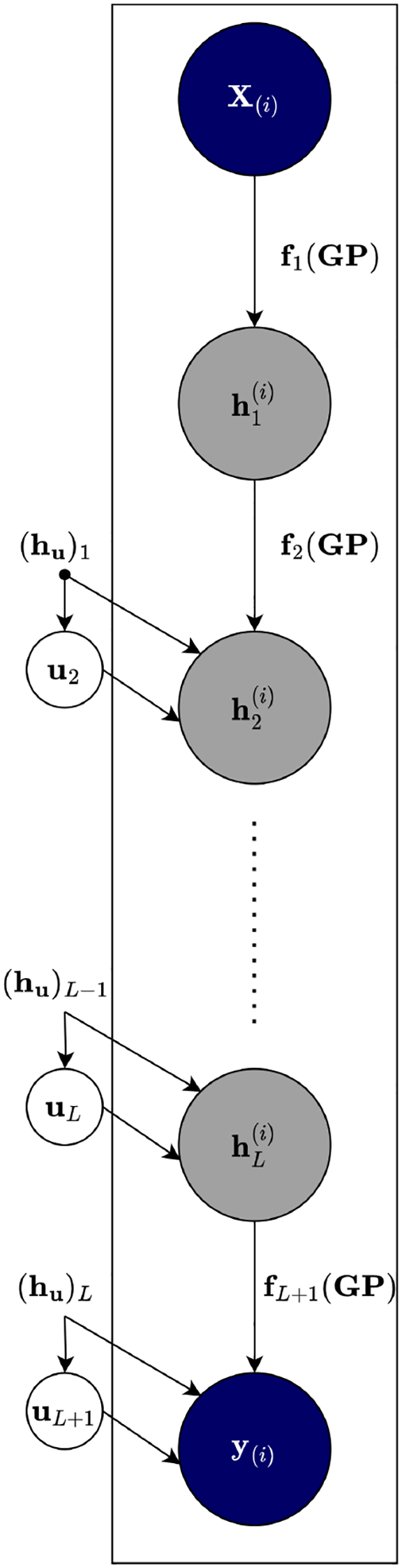
Graphical representation of a supervised deep GP model with inducing variables and L hidden layers, where inputs (X) propagate through latent layers (hi) to predict outputs (Y).
In the context of hydro-morphodynamic modeling, these latent layers can represent compressed but physically meaningful transformations of key processes, such as evolving flow velocities, suspended sediment transport, or morphodynamic bed changes across space and time.
This layered construction enables scalable and flexible modeling of complex non-linear dependencies across high-dimensional input–output spaces.
3.1 Bayesian GPLVM for probabilistic dimension reduction
To efficiently train deep GP models on high-dimensional hydro-morphodynamic data, it is essential to reduce the output space while retaining key non-linear dependencies and associated uncertainties. We employ the Bayesian Gaussian Process Latent Variable Model (Bayesian GPLVM), which offers a probabilistic and scalable framework for dimensionality reduction.
The Bayesian GPLVM captures non-linear structures within data while providing uncertainty quantification through a fully probabilistic mapping. To manage complex datasets efficiently, sparse approximations based on inducing variables are employed, reducing computational demands. In this application, the latent variables learned via GPLVMs allow us to discover a low-dimensional but physically consistent representation of complex hydrodynamic and sedimentary patterns driven by mangrove-root interactions. Accordingly, the true posterior distribution over latent variables is intractable. Instead, we approximate it using a variational posterior, i.e., a simpler, tractable distribution optimised to be close to the true posterior. This variational approximation enables scalable Bayesian learning for high-dimensional problems.
A detailed account of the generative mapping, covariance structures, prior assumptions, and variational inference methodology is provided in the Supplementary File, Sections 4–6.
3.2 Training a deep Gaussian process model
Training a deep GP model involves recursively applying GP mappings and GPLVM-based dimension reduction across L hidden layers, proceeding from the observed outputs Y toward the inputs X.
The main training steps are as follows:
-
1. Initialization: Given observed output data Y, apply GP regression to:
a. Generate the latent variable with dimension ,
b. Approximate the posterior distribution ,
c. Construct the data matrix for subsequent layers.
-
2. Recursive Inference: Given , apply Bayesian GPLVM to:
a. Generate the latent variable with dimension ,
b. Approximate the variational posterior
c. Propagate the reduced data .
-
3. Layer-wise Composition: Repeat this process to generate and their corresponding variational posterior distributions.
-
4. optimisation: The model parameters (e.g., kernel hyperparameters, noise variances) and variational parameters are optimised by maximising the variational lower bound on the marginal likelihood .
-
5. Final Model: The fully trained deep GP model corresponds to the composition given in Equation 4, enabling prediction and uncertainty quantification tasks.
In this study, kernel hyperparameters and noise variances were initialised using the automatic relevance determination (ARD) kernel and optimised by maximising the evidence lower bound (ELBO) through a gradient-based optimiser (Adam). The number of inducing points m was chosen empirically (m ≪ n) to balance accuracy and computational efficiency, reducing the computational complexity from O(n3) to O(nm2).
Through this training process, the model learns a hierarchical mapping from input drivers such as tidal forcings, bed topography, or vegetation parameters to dynamic hydro-morphodynamic responses across space and time.
A detailed pseudocode of the variational inference procedure, including parameter updates for the mean and covariance of the variational posteriors, is provided in Algorithm 1 and Equations S12–S18 of the Supplementary Material to ensure reproducibility. Full details of the variational inference algorithm and training procedure are provided in Section 2, particularly Algorithm 1 of the Supplementary File. For completeness, the Supplementary Material (Appendices 1–3) also describes the use of the ARD kernel, the sparse variational formulation with inducing variables, and the gradient-based optimisation of the ELBO that govern the training process.
3.3 Prediction with deep Gaussian processes
To achieve dimensionality reduction before prediction, the Bayesian GPLVM was employed to map the high-dimensional model outputs onto a lower-dimensional latent space while preserving probabilistic uncertainty.
The latent dimensionality q was determined using the optimised ARD weights, which indicated a single dominant component with the remaining dimensions contributing negligibly. To ensure that no key physical information was lost, we verified the reconstruction quality by comparing the GPLVM-reconstructed hydro- morphodynamic fields with the original numerical outputs. This comparison, documented in Section 5 (Figures 2, 3), shows close agreement between the reconstructed and simulated fields, confirming that the reduced latent representation retains the dominant physical behaviour while significantly reducing computational cost.
Figure 2
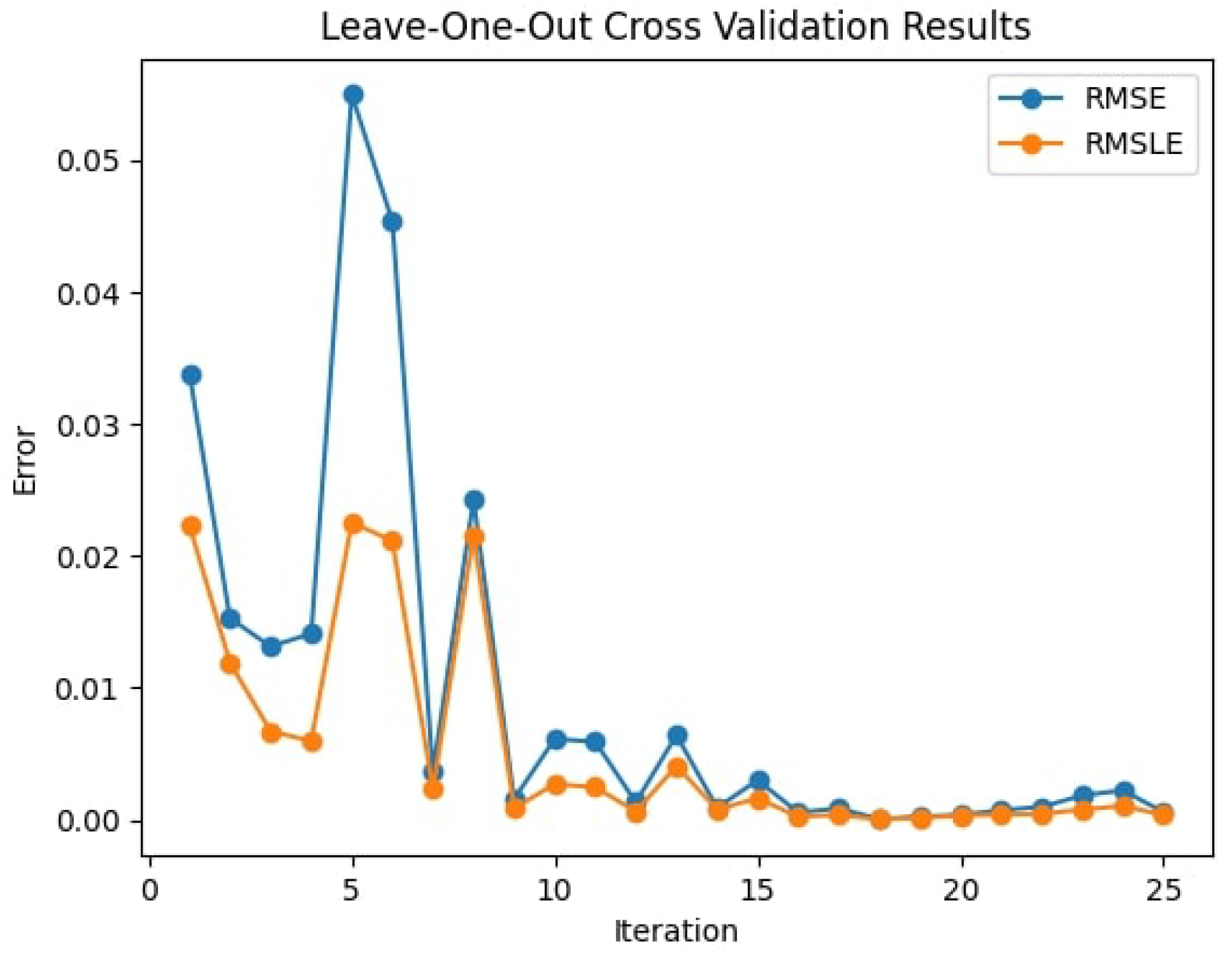
Leave-one-out cross-validation errors (RMSE and RMSLE) for the deep GP across 25 time-steps, highlighting improved accuracy and consistency over time.
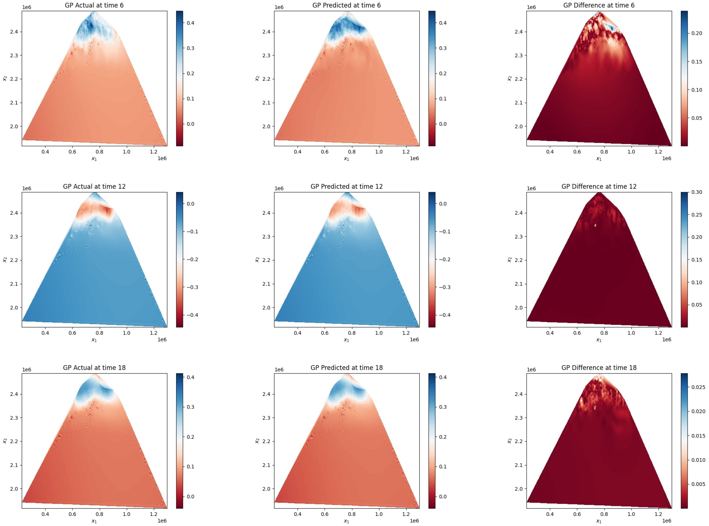
Figure 3
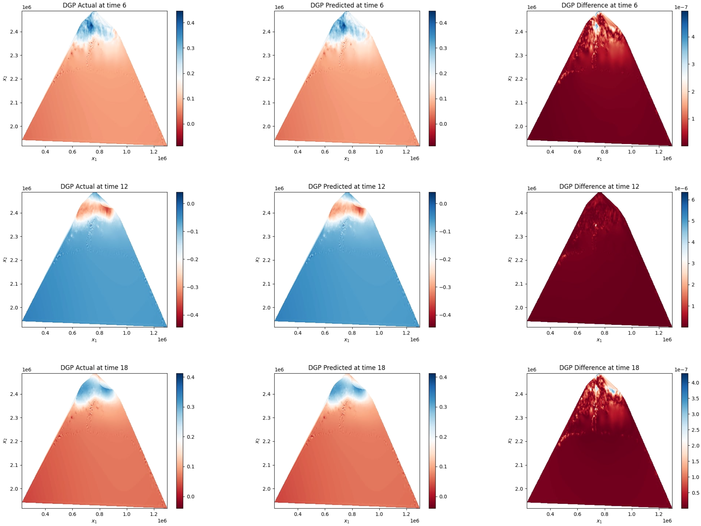
Comparison of deep GP predicted vs actual elevation outputs at 6, 12, and 18 hours. The left column shows the actual elevation obtained from the numerical model, the middle column presents the corresponding deep GP predictions, and the right column illustrates the absolute differences (errors) between them. Blue to red color bars in the first two columns indicate elevation values (e.g., low to high elevation), while the error maps use a red hue to denote magnitude of residuals, with darker shades representing higher discrepancies. The low intensity of residuals confirms the high accuracy of the deep GP emulator across space and time.
Once trained, the deep GP model predicts the output for a new test input by recursively propagating uncertainty through the latent layers. At each layer, the predictive distributions are computed using the corresponding GP posterior learned during training.
The main predictive steps are:
1. First Layer Prediction:
a. Compute ,
b. Approximate with predictive mean and variance.
2. Recursive Propagation: For each layer :
a. Compute ,
b. Approximate recursively.
3. Final Output Prediction:
a. Use the final latent variable to predict ,
b. Derive the predictive mean and variance of .
This uncertainty-aware prediction allows us to estimate future water elevations, sediment distributions, or morphological changes under new forcing conditions, while quantifying the associated confidence intervals.
This recursive prediction framework forms the basis for the uncertainty propagation methodology presented in Section 4. Full derivations for computing the predictive distributions at each layer can be found in Sections 3–5 of the Supplementary Material (Appendices 1–3).
4 Uncertainty quantification using deep Gaussian processes
In this section, we extend the classical uncertainty quantification (UQ) framework proposed by Oakley and O’Hagan (Oakley and O’hagan, 2002) to the Deep GP setting. Building on ideas from (Bilionis et al., 2013; Chatrabgoun et al., 2022), we present a sampling-based approach to efficiently propagate uncertainty through the trained deep GP model and estimate statistics of interest.
Specifically, our method generates Monte Carlo realisation from the variational posterior distributions at each latent layer. These realisations are then recursively propagated through the deep GP structure to estimate quantities of interest (QoIs), such as the mean and variance of the model output y.
Algorithm 1 is summarised below.
Algorithm 1
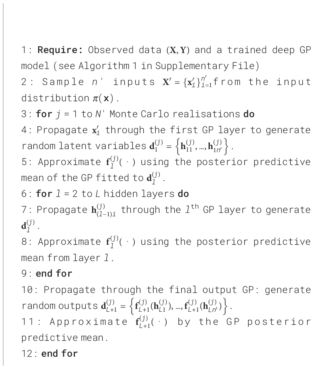
Once Monte Carlo samples are generated, we can estimate QoIs.
For instance, the expectation of the model output y for realisation j is given by:
which is approximated numerically using Monte Carlo integration:
Repeating this process over N′ Monte Carlo realisations produces a sample from the distribution of the model mean E(Y).
Remark 1: It is important to clarify that the Monte Carlo (MC) integration employed within the proposed framework differs fundamentally from conventional MC-based UQ approaches. In traditional settings, each MC sample requires a full evaluation of the underlying numerical model, which becomes computationally infeasible for complex hydro-morphodynamic simulations. In contrast, the present framework utilises samples drawn from the predictive distribution of the trained Deep GP surrogate. This allows for rapid generation of realisations at negligible cost, while still capturing model-form (epistemic) and predictive uncertainties encoded in the surrogate. Consequently, although the sampling procedure formally resembles MC integration, the underlying computational burden is substantially reduced, enabling scalable UQ for high-dimensional and nonlinear systems.
Similarly, the Monte Carlo samples can be used to approximate variances, credible intervals, or other summary statistics of Y.
Remark 2: This probabilistic UQ framework is particularly suitable for hydro-morphodynamic modeling, where uncertainties in inputs such as tidal forcing, sediment properties, or vegetation density propagate through complex nonlinear processes to affect outputs such as water surface elevation, flow velocity, and morphological evolution. The use of Deep GP models allows for efficient and uncertainty-aware predictions even in high-dimensional settings, thereby supporting robust decision-making for coastal protection and mangrove ecosystem resilience.
The following section applies the proposed Deep GP framework and the UQ strategy outlined above to the mangrove hydro-morphodynamic case study, enabling a direct evaluation of predictive accuracy, uncertainty behaviour, and computational performance.
5 Uncertainty quantification for hydro-morphodynamic model
This section presents the model evaluation and uncertainty quantification results obtained by applying the methodology described in Sections 3 and 4 to the Sundarbans hydro-morphodynamic domain. We evaluate the proposed UQ framework in the context of the depth-averaged Navier–Stokes system introduced in Section 2 and begin by introducing the study area and its relevance to coastal resilience modelling.
5.1 Study area context
This study focuses on the Indian Sundarbans, the largest contiguous mangrove forest in the world, located at the confluence of the Ganges, Brahmaputra, and Meghna rivers. This region, shared between India and Bangladesh, is critically endangered due to accelerated sea-level rise, tropical cyclones, and anthropogenic pressure.
The study domain includes the deltaic islands and tidal channels of the Indian Sundarbans, extending from Sagar Island in the west to the Ichhamati-Raimangal estuary in the east. The area has witnessed considerable shoreline retreat, with net erosion rates exceeding 5 m/year in some zones (Mondal et al., 2025). Tidal influences, sediment dynamics, and seasonal monsoons dominate the hydro-morphodynamic processes of this low-lying ecosystem.
Previous studies have shown that changes in bathymetry and shoreline position directly impact mangrove survival and regeneration (Hossain et al., 2022). Hence, accurate modeling of elevation dynamics is essential for assessing future ecosystem vulnerability under climate change scenarios.
Our primary focus is on the Sundarbans mangrove forest situated between India and Bangladesh, as detailed in (Fanous et al., 2023c). The modeled region of interest covers the entire Bay of Bengal shelf, including the Sundarbans mangrove forest (Figure 4). Employing a spatially varying mesh resolution, we capture tidal wave dynamics from the Indian Ocean to the mangroves, varying from 8 km to 1.5 km (Figure 5).
Figure 4
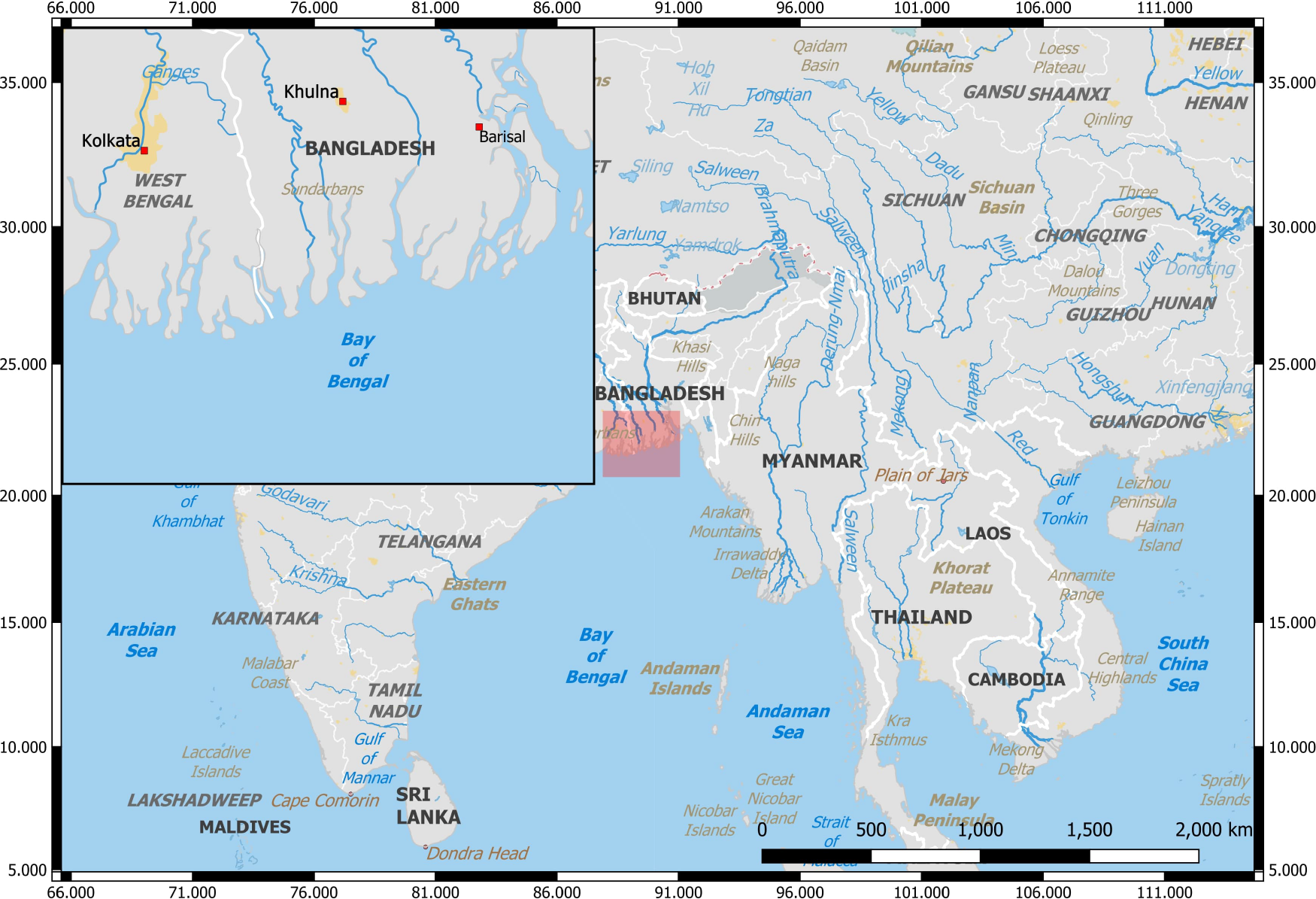
Model domain covering the Bay of Bengal shelf, with a focus on the Sundarbans mangrove forest located between India and Bangladesh. The inset highlights regional river systems and urban centers influencing the hydro-morphodynamic environment.
Figure 5
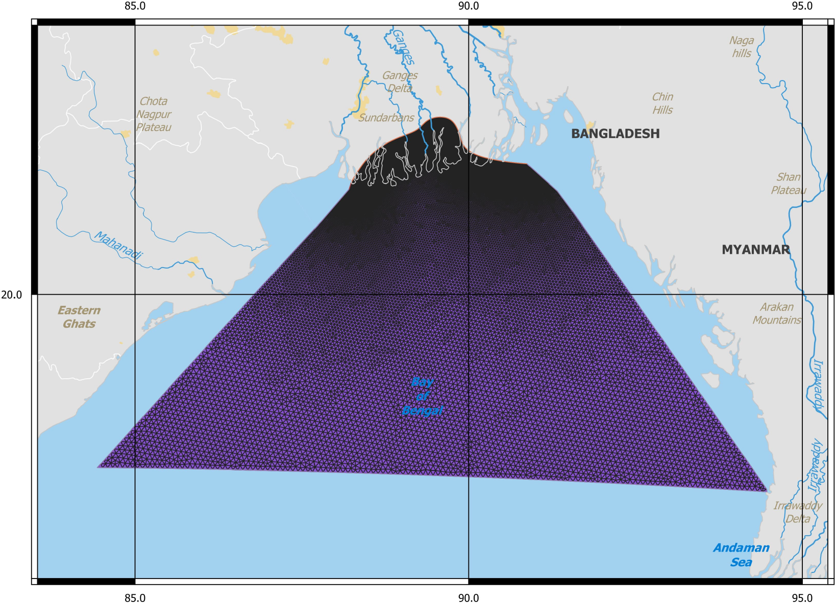
Computational mesh over the Bay of Bengal shelf generated using Gmsh, with resolution varying spatially from 8 km offshore to 1.5 km near the Sundarbans mangrove region.
Focusing on the Sundarbans region, which is confronted with imminent threat of rising sea levels, there is a pressing need for precise modeling to gain a deep understanding of mangrove dynamics under various climate change scenarios (Fanous et al., 2023b). Accurate hydro-morphodynamic modeling is essential for planning NbS that can sustain mangrove ecosystems under future climate pressures. The quantification of the uncertainties can help decision-makers design resilient strategies to protect coastal zones and communities (Kent et al., 2024). Employing both the conventional single-layer GP and adopted deep GP models as surrogates for replacing the previously developed numerical model (Fanous et al., 2023a), we aim to comprehensively compare the capabilities of both of these models for accurately and efficiently predicting the change of elevation over time and quantifying the uncertainty for such predictions.
5.2 Validation metrics
In this section, we introduce two metrics required to examine the performance of the fitted GP and deep GP models to the data of the numerical model. Subsequently, we comprehensively evaluate the proposed UQ of both methods when applied to hydro-morphodynamic modeling of the case study discussed above. The inputs to these models consist of time, while the outputs represent the elevation across the spatial domain for each timestep. The resulting dimensions for inputs and outputs are and , respectively. This represents 25 aggregated time-steps across all simulations and 19,285 features (cells) for each timestep.
To validate and assess out-of-sample performance, we employ the leave-one-out cross-validation (LOOCV) method. In this approach, the GP-based emulator is trained on 24 time-steps, and its predictive performance is evaluated on the remaining timestep. This process is iteratively repeated for all 25 training examples. Choosing this validation method allows us to examine the model’s robustness against limited data and across diverse spatial configurations and complexities. This robust validation approach ensures that surrogate models maintain predictive accuracy across a variety of hydro-morphodynamic scenarios, a vital requirement for real-world application to coastal adaptation planning.
For accuracy evaluation, we utilize the root mean squared error (RMSE) and the root mean squared log error (RMSLE), defined by the following equations:
where n is the number of observations, is the actual value, and is the predicted value.
Furthermore, we provide visual illustrations of the performance of both models across different time-steps to examine the spatial and temporal prediction capabilities. Finally, we assess uncertainty quantification (UQ) for both approaches using the methodology outlined in Section 4.
These analyses validate the predictive performance of the surrogate models and provide a crucial foundation for evaluating how uncertainty evolves across time and space in complex coastal systems. The enhanced understanding of predictive uncertainties contributes toward establishing more reliable nature-based coastal defenses, directly supporting climate resilience planning for vulnerable ecosystems such as the Sundarbans. By quantifying the level of confidence in elevation and flow predictions under different conditions, our results deliver actionable insights for decision-makers aiming to implement adaptive, ecosystem-based management strategies in coastal zones.
5.3 Deep GP training and automatic feature selection
A deep GP with two hidden layers is used to approximate the complex mapping between the inputs and outputs given the observed data. The covariance function in Equation 3 is used with different length scales. Using this function, an automatic relevance determination (ARD) is applied, where very small weights of the dimensions of each latent space are discarded. The length scales () of this covariance function are automatically derived by training the deep GP model using the Bayesian variational method discussed in the previous section.
As explained in Algorithm 1 of the Supplementary File, training of the deep GP model starts by reducing the dimensionality of the model output using a Bayesian GPLVM. The model is then trained by optimising the lower bound of , given in Equation S13, using the Bayesian variational method. Figure 6 shows the optimised ARD weights after the application of the BGPLVM, indicating that most output dimensions were effectively reduced to near-zero, with one dominant dimension carrying most of the variance.
Figure 6
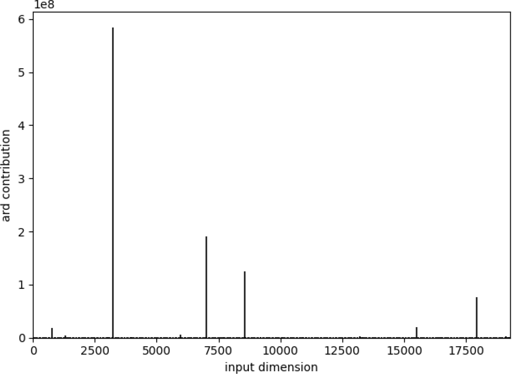
Optimised ARD weights obtained after applying the Bayesian GPLVM during deep GP training. The plot shows that most output dimensions contribute negligibly to the variance, while a few dominant dimensions carry most of the information.
After reducing the dimensionality of the outputs, the deep GP model fits the inputs to the dimensionality reduced outputs. Finally, the predicted output is constructed from the latent predictions through a final GP layer. The mean RMSE and RMSLE values are 0.0095 and 0.0052 respectively, which demonstrate substantial abilities of this model to accurately emulate the numerical model.
These results underline the potential of applying data-efficient machine learning methods to hydro-morphodynamic modeling tasks, which are critical for projecting the future stability of mangrove ecosystems under sea-level rise scenarios. Accurate emulation of complex processes is vital for assessing the resilience of natural coastal defenses.
Figure 2 shows the test RMSE and RMSLE values for each iteration. As anticipated, the RMSLE values are less than the RMSE, suggesting that they theoretically provide a more accurate estimation of the model’s error as it better targets the underestimation of the prediction. There are some noticeable variances in the error especially at the beginning of the model. The variation at the beginning can be explained with the time-dependent nature of the data, the prediction of the current timestep depends on the previous timestep. Thus, as there was not enough data for the earlier time-steps, the resulted error was a bit higher compared with the subsequent time-steps. Nonetheless, a consistent performance is evident across the majority of the test cases.
Such consistency across multiple time-steps demonstrates that the deep GP model is robust enough to support dynamic adaptation strategies for mangrove-based NbS, where hydrodynamic and morphological responses evolve over time under climatic stressors.
To have a closer inspection at the performance of the model across the spatial domain, Figure 3 shows the predicted elevation from the deep GP versus the actual modeled elevation using the numerical model and the difference between both at different times. From these figures, it can be evidently shown the significant accuracy for the deep GP model and its ability to accurately map the inputs to the outputs and to reconstruct the full dimensional output space from the latent space.
Accurately mapping spatial patterns of elevation change is especially important for the Sundarbans, where micro-topographic variations directly control tidal flushing, salinity intrusion, and seedling establishment, all fundamental processes for mangrove health and shoreline protection. Thus, ensuring spatially coherent and uncertainty-quantified predictions is crucial for long-term climate adaptation strategies.
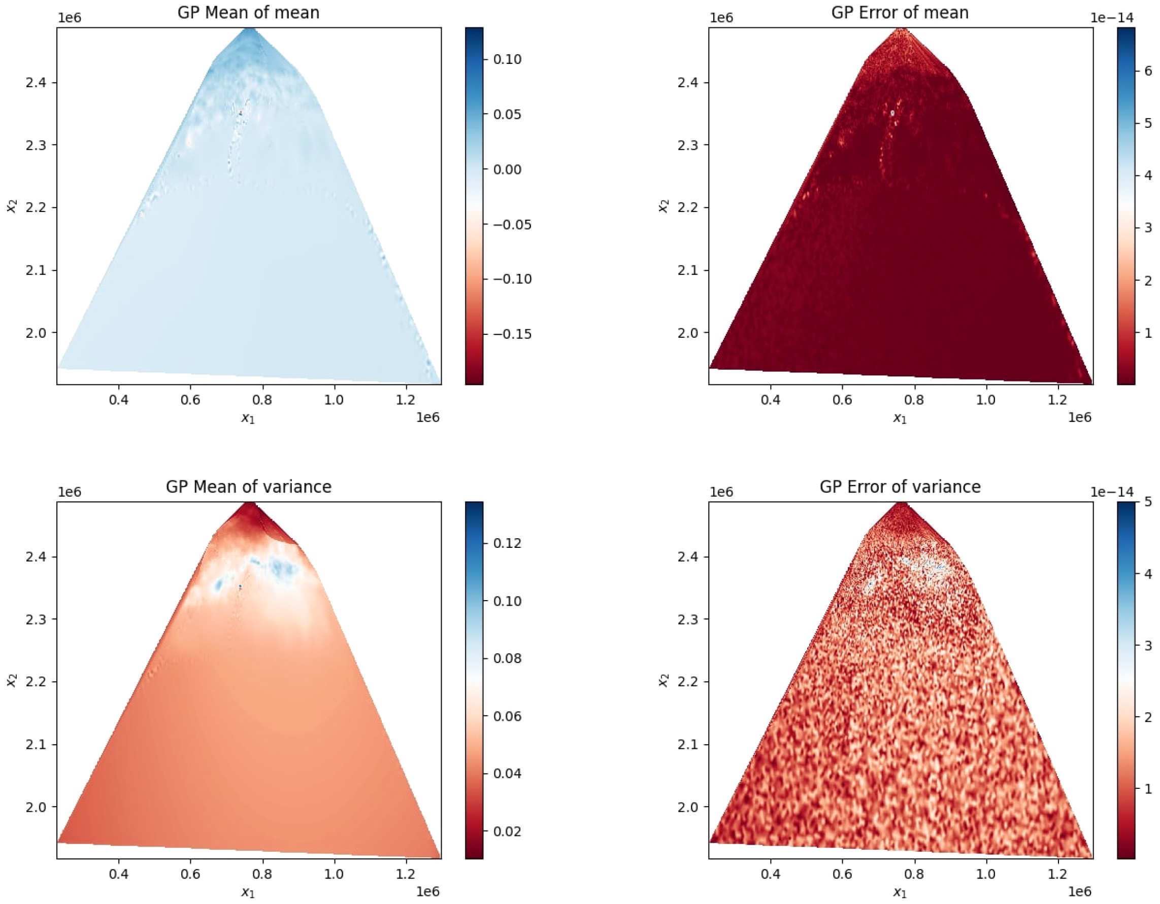
Using the UQ algorithm presented in Section 4, we estimate the mean of the predictive mean and the mean of the predictive variance of the deep GP model, along with their respective approximation errors. Figure 7 displays these quantities, computed using 10,000 Monte Carlo samples: the top row shows the mean of the predictive mean (left) and its associated error (right), while the bottom row presents the mean of the predictive variance (left) and the corresponding error (right). These results highlight the effectiveness of the deep GP model in capturing and propagating uncertainty across the domain. In the context of climate adaptation planning, reliable quantification of predictive uncertainty ensures that decision-makers can
Figure 7
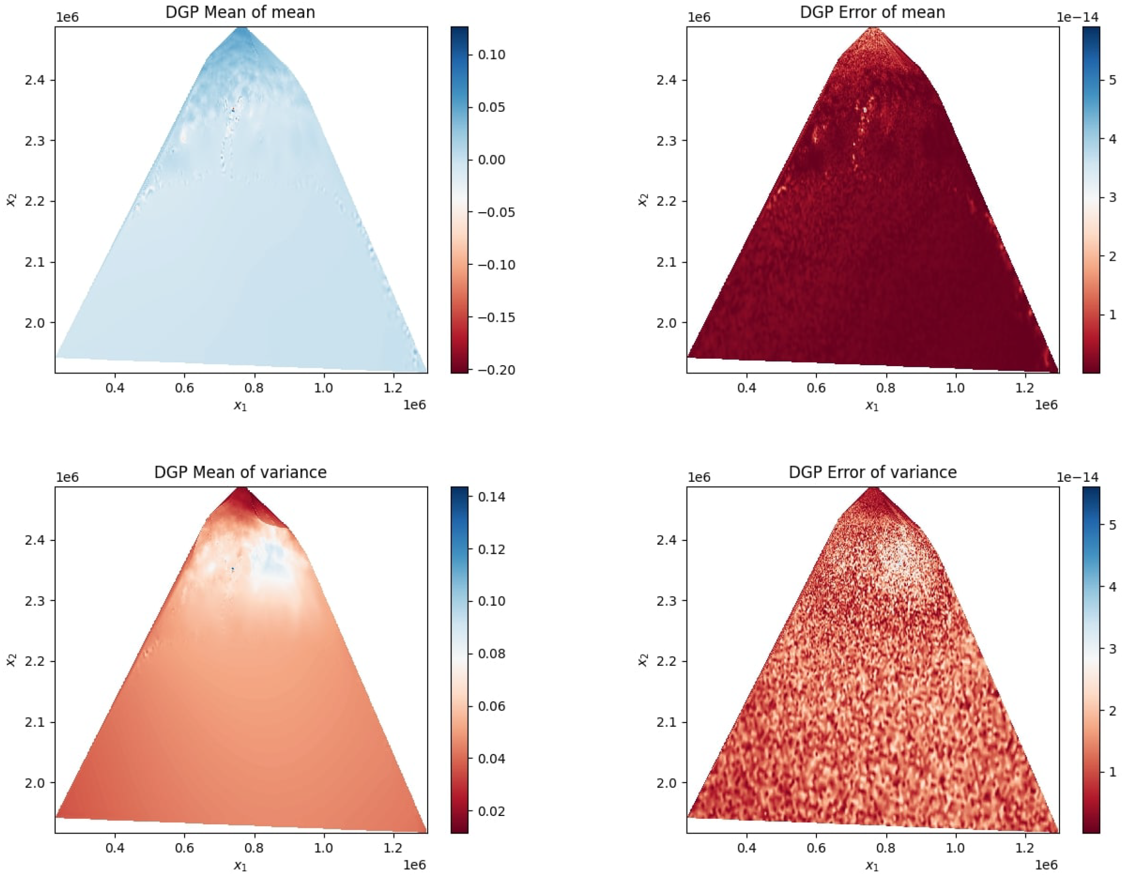
UQ results using the deep GP model based on 10,000 samples. Top left: Posterior mean of the predictive mean. Top right: Error in the posterior mean (numerical approximation error). Bottom left: Posterior mean of the predictive variance. Bottom right: Error in the predictive variance. All results are shown over the spatial domain (x1,x2).
account for model confidence when designing protective infrastructure, selecting conservation zones, or projecting mangrove migration patterns under sea-level rise.
Spatially, uncertainty is highest near channel bifurcations and shore–vegetation interfaces, where hydrodynamic gradients and sediment transport rates exhibit strong variability, and lowest in deeper or morphodynamically stable regions.
Furthermore, a random point was selected, and its probability density function (PDF) was plotted and is shown in Figure 8. From this plot, it can be noticed the tight bounds of the two standard deviations are very close to the mean of the distribution (dotted line). This means that there is a low variability in the data and ensures the robustness of the deep GP model.
Figure 8
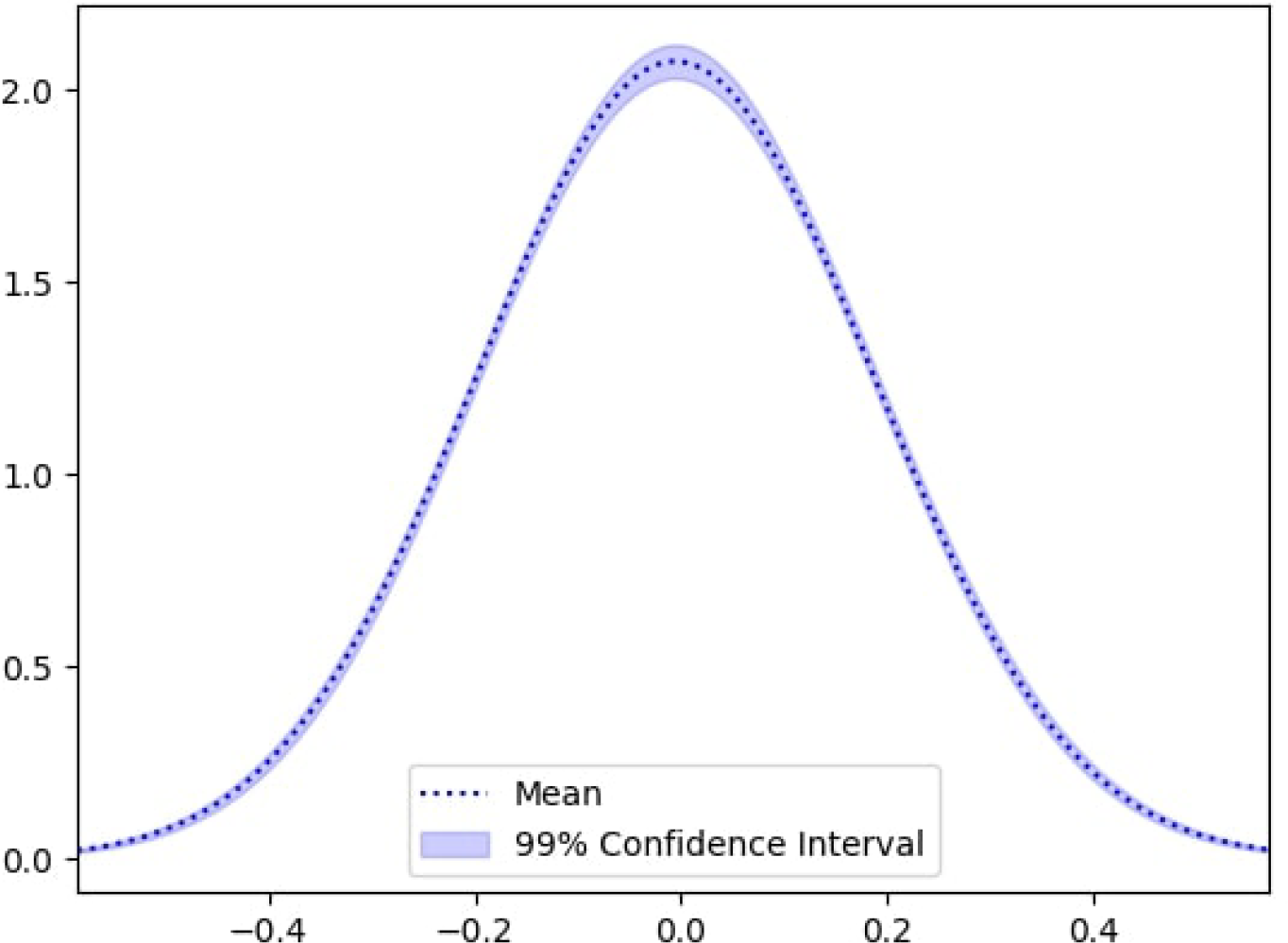
PDF of the model prediction at a selected spatial location for the deep GP. The black dashed line indicates the predictive mean, while the shaded blue region represents the 99% confidence interval. The narrow spread illustrates the model’s low predictive variance and strong robustness at that point.
Temporally, uncertainty increases during periods of rapid change in water levels and decreases when the system approaches more stable hydrodynamic conditions, as reflected in the variability patterns shown in Figure 8.
Finally, regarding the run-time of the deep GP model, it took 1 minute and 12 seconds for the model to develop the latent space from the high dimension output space, 30 seconds to train and test the model on the latent space, and 1 second to reconstruct the high dimension output space for a total of 1 minute and 43 seconds. This is over 3 orders of magnitude faster than the numerical model which validates the use of emulators to speed up the computation.
Such computational savings are significantly valuable from a research perspective. Nonetheless, they are also critical for operational management in coastal areas, where frequent scenario analyses and rapid decision-making under uncertainty are necessary to safeguard mangrove ecosystems and their protective functions.
5.4 Comparative evaluation: standard GP vs deep GP performance
Building on the UQ methodology introduced in Section 4, we systematically evaluate the predictive uncertainty of the Deep GP emulator by analysing the predictive medians, interquartile ranges, and 95% uncertainty bounds across selected spatial transects and temporal nodes.
We compared the performance of the deep GP model against the standard GP. The latter used the RBF kernel and same training/testing procedure. The mean RMSE and RMSLE for the GP model were 0.0465
and 0.0466 respectively. This shows, when compared to the deep GP, that the latter was 5 times more accurate than the standard GP model. Figure 9 shows the performance of the GP model on different training and testing validation sets. A similar comparison can be made for each of the validation sets, where the earlier time-steps had a much larger error compared to those for the deep GP. This shows the capabilities of the deep GP in modeling outputs without having a large number of data from previous time-steps. This allows for flexibility in the model and the ability to explore complex outputs accurately.
Figure 9

Leave-one-out cross-validation errors (RMSE and RMSLE) for the GP model across 25 timesteps, highlighting improved accuracy and consistency over time.
This level of flexibility is essential when dealing with coastal and estuarine environments like the Sundarbans, where temporal dynamics such as tides, sediment transport, and vegetation responses evolve continuously and need to be captured accurately to inform sustainable management of mangrove-based protection strategies.
Moving on, we plot the same data at times 6, 12, and 18 hours for elevation and its predicted output by the GP in Figure 10
Figure 10
Comparison of GP-predicted vs actual model outputs and corresponding differences at 6, 12, and 18 hours, analogous to the deep GP results shown in Figure 3.
From these figures, although the GP model is accurate, the errors are exacerbated compared to the deep GP errors as the maximum error for GP reached 0.3m compared to the 1e−6 by the deep GP which is a 5 order of magnitude improvement.
Such large discrepancies, even though moderate in traditional engineering applications, can significantly misrepresent the subtle yet crucial morphological changes occurring in vulnerable mangrove regions. A few centimeters of elevation error may dramatically affect predictions of tidal inundation patterns, seedling survival, and erosion control potential, highlighting the critical need for advanced UQ methods like the deep GP in NbS planning.
Regarding the UQ analysis, the mean of the predictive mean, the mean of the predictive variance, and their corresponding approximation errors were computed using the deep GP methodology introduced in Section 4. The top row of Figure 11 presents the posterior mean of the predictive mean (left) and the
Figure 11
UQ results using the GP model based on 10,000 samples. Top left: Posterior mean of the predictive mean. Top right: Error in the posterior mean (numerical approximation error). Bottom left: Posterior mean of the predictive variance. Bottom right: Error in the predictive variance. All results are shown over the spatial domain (x1,x2).
It can be noticed that the performance of both models is quite similar, however, there are slight better improvements on the mean of the variance where the GP model had a large area of variance compared to the GP. These results confirm the ability of deep learning architectures to tackle complex predictive tasks and provide an accurate measure of uncertainty.
From an environmental perspective, tighter variance control in predictions is crucial for designing adaptive management policies, as it reduces the risk of over- or under-estimating the effectiveness of mangrove-rooted barriers in storm surge mitigation, sediment retention, and shoreline stability.
Similarly, the PDF of a random point is shown in Figure 12. In comparison to PDF plot of the deep GP model in Figure 8, the PDF of the GP shows a higher degree in variability.
Figure 12
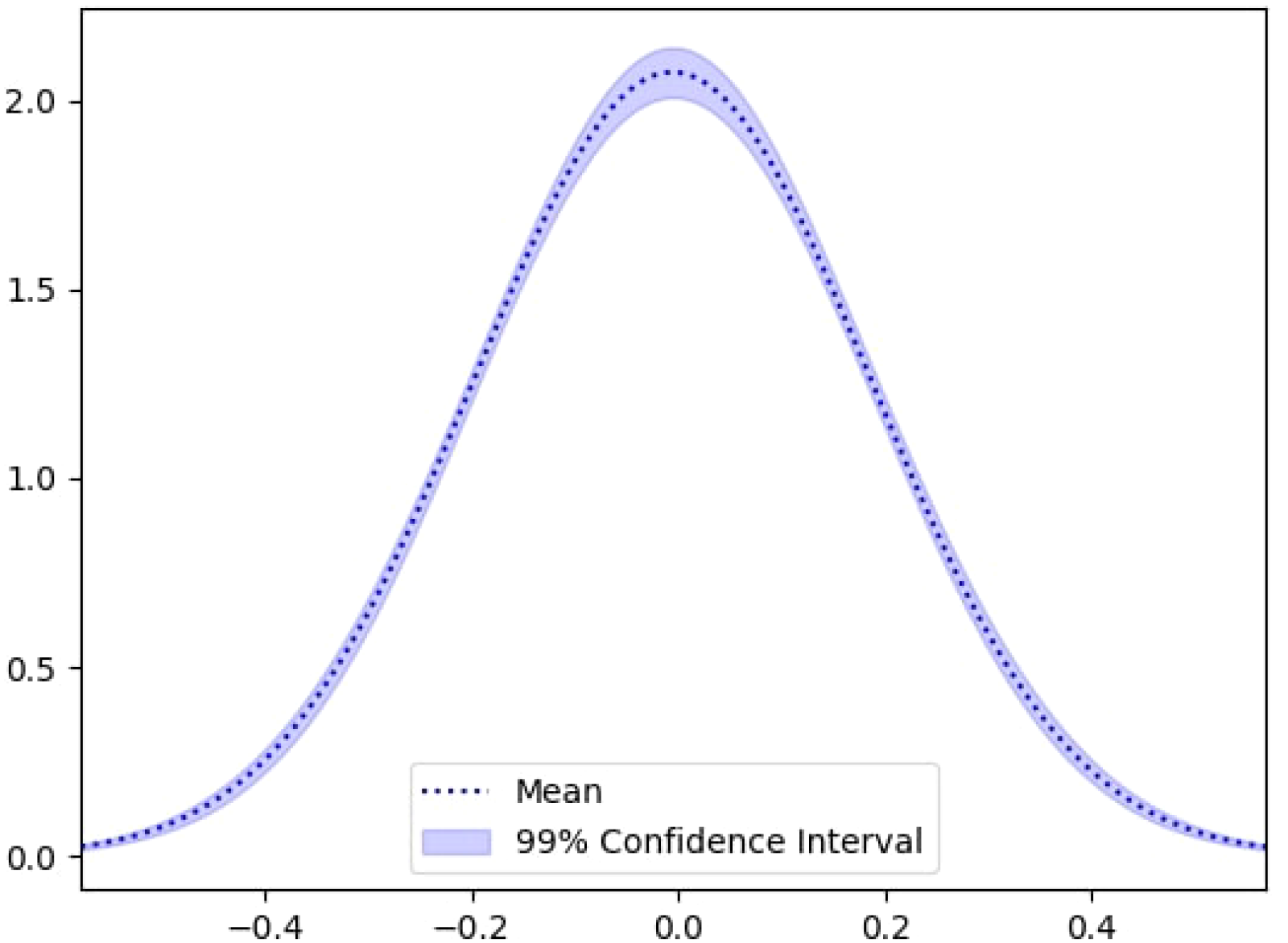
PDF of the model prediction at a selected spatial location for the standard GP model. Similar to Figure 8 for the deep GP, the black dashed line indicates the predictive mean and the shaded blue region shows the 99% confidence interval. Compared to the deep GP, the GP model exhibits slightly wider uncertainty bounds, indicating higher predictive variance and less robustness at the same location.
Finally, regarding the run-time of the GP model, the model took just 16 seconds to run the training and testing procedure which is, as expected, faster than the deep GP model. This difference in the computation time between both models is due to the more complex operations run by the deep GP as it constructs a latent space and has more layers, thus more parameters, to optimise. Nonetheless, the run-time of the deep GP is still substantially better than the numerical model, and the accuracy of the deep GP is much better than the GP.
The modest additional computational effort required for the deep GP is a worthwhile tradeoff, considering the significant improvements in uncertainty control, especially for NbS applications where minimising errors and uncertainty can lead to more resilient and sustainable coastal adaptation solutions.
The advantages of the Deep GP framework arise from its hierarchical structure, which allows the model to represent multi-scale nonlinearities and non-Gaussian dependencies more effectively than standard GPs or shallow surrogate models. Each layer captures residual structure unexplained by the previous layer, enabling the emulator to learn complex hydro-morphodynamic interactions such as shoreline–vegetation feedbacks and spatial gradients in flow and sediment transport. In contrast to deep neural networks or PINNs, Deep GPs retain a fully Bayesian formulation that naturally propagates uncertainty through the model, providing calibrated predictive intervals while avoiding the risk of overconfident extrapolation.
Compared with other advanced surrogate approaches, such as PINNs (Raissi et al., 2019), Bayesian PINNs (Yang and Foster, 2022), and polynomial chaos expansions (Wan and Karniadakis, 2005; Li et al., 2021), the Deep GP demonstrates more favourable trade-offs between accuracy, robustness, and computational cost. PINN-based methods can embed physical constraints but often suffer from optimisation difficulties and scalability limitations in large coastal domains (Fanous et al., 2023a, b), whereas polynomial chaos methods become inefficient in the presence of strong nonlinearities and high-dimensional parameter spaces. The Deep GP, by contrast, remains tractable through sparse variational inference (Titsias and Lawrence, 2010) and generalises well across spatial domains. Although the present study focuses on one mangrove system, the underlying drivers, vegetation–flow interactions, sediment feedbacks, and channel complexity, are shared across many mangrove ecosystems (Mazda et al., 2005; Gilman et al., 2008). This suggests the framework is likely to be transferable to other sites, provided site-specific forcings and boundary conditions are incorporated during training.
6 Conclusions and future works
6.1 Major findings
This study presents a novel methodology for efficiently implementing UQ in complex hydro- morphodynamic models using deep GPs. The framework demonstrates substantial improvements over traditional surrogate models by offering both higher predictive accuracy and drastically reduced computational cost. It successfully captures the intricate, nonlinear interactions inherent in spatio-temporal coastal processes and produces robust UQ outputs. Deep GPs consistently outperform standard GP models, especially when modeling high-dimensional outputs across large spatial domains. The integration of Bayesian GPLVM enables automatic dimensionality reduction, leading to better computational scalability and generalisability. These capabilities are particularly relevant in the context of NbS for coastal resilience, such as mangrove protection systems.
Beyond methodological contributions, the Deep GP framework also offers practical value for coastal management and NbS planning. The ability to rapidly generate uncertainty-aware predictions enables decision-makers to assess confidence levels in projected water elevations, identify zones of elevated risk, and prioritise areas where mangrove restoration or protective interventions may have the greatest impact. Spatial maps of predictive variance can guide surveillance and monitoring efforts by highlighting regions where additional data would most reduce uncertainty. Furthermore, temporal UQ outputs allow coastal planners to evaluate scenario robustness under extreme hydrodynamic conditions, supporting adaptive management strategies such as early-warning thresholds, optimisation of restoration layouts, and design of resilient buffer zones. These examples demonstrate how the proposed UQ framework can directly inform operational decisions in climate-exposed coastal regions.
6.2 Research limitations
While the proposed deep GP approach is efficient and accurate, several limitations persist. The surrogate model requires retraining when major changes in initial or boundary conditions occur, which can involve additional computation and setup time. Moreover, deep GPs rely on variational inference as exact Bayesian solutions are analytically intractable, introducing possible approximation errors. Another critical issue is the lack of inherent physical interpretability in deep GPs; without embedded physical constraints, the model may generate predictions that are statistically sound but physically implausible. This limits their direct applicability in high-stakes decision-making unless complemented by domain-specific knowledge or hybrid methods.
A further limitation relates to the volume and diversity of training data required for capturing the full range of hydro-morphodynamic variability. Although the present Deep GP model performs well with the available simulation ensemble, its performance may degrade in settings where the training data do not sufficiently cover rare or extreme events, or where the parameter space is substantially broader. In such cases, the model may under-represent tail behaviour or exhibit wider predictive uncertainty, particularly in highly nonlinear regions of the state space. These constraints reflect a general challenge shared by most surrogate models, including PINNs, Bayesian PINNs, and polynomial chaos expansions.
6.3 Recommendations for future research
Future research should focus on strengthening the robustness and generalisability of the proposed Deep GP framework. First, the performance of the surrogate remains sensitive to the volume and diversity of the training data. Targeted sampling of rare or extreme conditions, along with adaptive enrichment of the training set, would help ensure reliable performance under rapid hydrodynamic transitions or climate-induced extremes. In addition, evaluating the model across mangrove and estuarine systems with differing geomorphological and ecological characteristics would provide insight into its universality and transferability.
Another promising direction is the hybridisation of Deep GPs with physics-informed modelling. Embedding conservation laws directly into the kernel design or variational objective could improve physical fidelity, particularly for long-term predictions or scenarios where observational constraints are limited. Such extensions would enhance model robustness compared with conventional surrogates, especially for multiscale PDE-based systems where numerical solvers are computationally expensive and shallow GP models struggle to capture the required dynamics.
Finally, the integration of online or transfer learning techniques represents an important opportunity for applications in dynamically evolving coastal systems. These approaches would enable rapid surrogate updates as new data become available, supporting real-time forecasting and operational decision-making in climate-resilient coastal management.
Supplemental data
The Supplementary Material for this article contains detailed mathematical derivations, variational inference formulations, training algorithms, and additional explanations supporting the methodology described in Sections 2–4 of the main manuscript. It is provided as a separate file and is available online at the journal website.
Readers are referred to the Supplementary Material for full technical details on the Bayesian GPLVM training, Deep GP model optimisation, and predictive uncertainty quantification procedures.
Statements
Data availability statement
The raw data supporting the conclusions of this article will be made available by the authors, without undue reservation.
Author contributions
MF: Writing – review & editing, Data curation, Formal Analysis, Visualization, Writing – original draft, Methodology, Validation, Software, Investigation, Conceptualization. HA: Resources, Writing – original draft, Methodology, Writing – review & editing. AH-F: Writing – review & editing, Investigation, Writing – original draft, Conceptualization. OC: Investigation, Writing – review & editing, Conceptualization, Writing – original draft, Formal Analysis, Methodology. TS: Methodology, Writing – original draft, Data curation, Writing – review & editing. AD: Writing – review & editing, Funding acquisition, Resources, Writing – original draft, Formal Analysis, Conceptualization, Methodology, Visualization, Validation, Supervision.
Funding
The author(s) declared that financial support was not received for this work and/or its publication.
Acknowledgments
The authors would like to thank Coventry University for funding this PhD Studentship titled “Enhancing Mangrove Forest Resilience against Coastal Degradation and Climate Change Impacts using Advanced Bayesian Machine Learning Methods”, through the GCRF Scheme.
Conflict of interest
The author(s) declared that this work was conducted in the absence of any commercial or financial relationships that could be construed as a potential conflict of interest.
Generative AI statement
The author(s) declared that generative AI was not used in the creation of this manuscript.
Any alternative text (alt text) provided alongside figures in this article has been generated by Frontiers with the support of artificial intelligence and reasonable efforts have been made to ensure accuracy, including review by the authors wherever possible. If you identify any issues, please contact us.
Publisher’s note
All claims expressed in this article are solely those of the authors and do not necessarily represent those of their affiliated organizations, or those of the publisher, the editors and the reviewers. Any product that may be evaluated in this article, or claim that may be made by its manufacturer, is not guaranteed or endorsed by the publisher.
Supplementary material
The Supplementary Material for this article can be found online at: https://www.frontiersin.org/articles/10.3389/fmars.2025.1624244/full#supplementary-material
References
1
Atkinson S. Zabaras N. (2019). Structured bayesian gaussian process latent variable model: Applications to data-driven dimensionality reduction and high-dimensional inversion. J. Comput. Phys.383, 166–195. doi: 10.1016/J.JCP.2018.12.037
2
Batsch F. Daneshkhah A. Cheah M. Kanarachos S. Baxendale A. (2019). Performance boundary identification for the evaluation of automated vehicles using gaussian process classification. 2019 IEEE Intelligent Transportation Syst. Conference ITSC2019, 419–424. doi: 10.1109/ITSC.2019.8917119
3
Bilionis I. Zabaras N. Konomi B. A. Lin G. (2013). Multi-output separable Gaussian process: Towards an efficient, fully Bayesian paradigm for uncertainty quantification. J. Comput. Phys.241, 212–239. doi: 10.1016/j.jcp.2013.01.011
4
Chang C.-W. Mori N. (2021). Green infrastructure for the reduction of coastal disasters: A review of the protective role of coastal forests against tsunami, storm surge, and wind waves. Coast. Eng. J.63, 370–385. doi: 10.1080/21664250.2021.1929742
5
Chatrabgoun O. Esmaeilbeigi M. Cheraghi M. Daneshkhah A. (2022). Stable likelihood computation for machine learning of linear differential operators with Gaussian processes. Int. J. Uncertainty Quantification12, 75–99. doi: 10.1615/INT.J.UNCERTAINTYQUANTIFICATION.2022038966
6
Clare M. C. A. Kramer S. C. Cotter C. J. Piggott M. D. (2022). Calibration, inversion and sensitivity analysis for hydro-morphodynamic models through the application of adjoint methods. Comput. Geosciences163, 105104. doi: 10.1016/j.cageo.2022.105104
7
Damianou A. (2015). Deep Gaussian processes and variational propagation of uncertainty. Ph.D. thesis. (Sheffield, UK: University of Sheffield).
8
Daneshkhah A. Bedford T. (2013). Probabilistic sensitivity analysis of system availability using gaussian processes. Reliability Eng. System Saf.112, 82–93. doi: 10.1016/j.ress.2012.11.001
9
Daneshkhah A. Hosseinian-Far A. Chatrabgoun O. (2017). “ Sustainable maintenance strategy under uncertainty in the lifetime distribution of deteriorating assets,” in Strategic engineering for cloud computing and big data analytics (Cham: Springer International Publishing), 29–50.
10
Dey S. (2014). Hydrodynamic principles (Berlin, Heidelberg: Springer Berlin Heidelberg), 29–93. doi: 10.1007/978-3-642-19062-92
11
Donnelly J. Abolfathi S. Pearson J. Chatrabgoun O. Daneshkhah A. (2022). Gaussian process emulation of spatio-temporal outputs of a 2d inland flood model. Water Res.225, 119100. doi: 10.1016/j.watres.2022.119100
12
Donnelly J. Daneshkhah A. Abolfathi S. (2024a). Forecasting global climate drivers using Gaussian processes and convolutional autoencoders. Eng. Appl. Artif. Intell.128, 107536. doi: 10.1016/j.engappai.2023.107536
13
Donnelly J. Daneshkhah A. Abolfathi S. (2024b). Physics-informed neural networks as surrogate models of hydrodynamic simulators. Sci. Total Environ.912, 168814. doi: 10.1016/j.scitotenv.2023.168814
14
Fanous M. Daneshkhah A. Eden J. M. Remesan R. Palade V. (2023a). Hydro-morphodynamic modelling of mangroves imposed by tidal waves using finite element discontinuous galerkin method. Coast. Eng.182, 104303. doi: 10.1016/J.COASTALENG.2023.104303
15
Fanous M. Daneshkhah A. Yang J. Eden J. M. See S. Palade V. (2023b). Physics informed neural networks to model the hydro-morphodynamics of mangrove environments. ECCOMAS Proceedia. 822–835. doi: 10.7712/120223.10378.19649
16
Fanous M. Eden J. M. Remesan R. Daneshkhah A. (2023c). Challenges and prospects of climate change impact assessment on mangrove environments through mathematical models. Environ. Model. Software162, 105658. doi: 10.1016/J.ENVSOFT.2023.105658
17
Fanous M. Eden J. Yang J. See S. Palade V. Daneshkhah A. (2025). Leveraging physics-informed neural networks for efficient modelling of coastal ecosystems dynamics: A case study of sundarbans mangrove forest. Ecol. Inf.90, 103302. doi: 10.1016/j.ecoinf.2025.103302
18
Franzen M. O. Fernandes E. H. Siegle E. (2021). Impacts of coastal structures on hydro morphodynamic patterns and guidelines towards sustainable coastal development: A case studies review. Regional Stud. Mar. Sci.44, 101800. doi: 10.1016/j.rsma.2021.101800
19
Giles M. (2008). “ Monte carlo and quasi-monte carlo methods 2006,” in chap. Improved multilevel monte carlo convergence using the milstein scheme ( Springer Berlin Heidelberg, Berlin, Heidelberg), 343–358. doi: 10.1007/978-3-540-74496-220
20
Gilman E. L. Ellison J. Duke N. C. Field C. (2008). Threats to mangroves from climate change and adaptation options: A review. Aquat. Bot.89, 237–250. Mangrove Ecology – Applications in Forestry and Costal Zone Management. doi: 10.1016/j.aquabot.2007.12.009
21
Harris D. L. Rovere A. Casella E. Power H. Canavesio R. Collin A. et al . (2018). Coral reef structural complexity provides important coastal protection from waves under rising sea levels. Sci. Adv.4, eaao4350. doi: 10.1126/SCIADV.AAO4350
22
Haun S. Dietrich S. (2021). Advanced methods to investigate hydro-morphological processes in open-water environments. Earth Surface Processes Landforms46, 1655–1665. doi: 10.1002/esp.5131
23
Hossain S. A. Mondal I. Thakur S. Al-Quraishi A. M. F. (2022). Coastal vulnerability assessment of India’s purba medinipur-balasore coastal stretch: A comparative study using empirical models. Int. J. Disaster Risk Reduction77, 103065. doi: 10.1016/j.ijdrr.2022.103065
24
Iman R. L. Conover W. (1980). Small sample sensitivity analysis techniques for computer models with an application to risk assessments. Commun. Stat - Theory Methods9, 1749–1842. doi: 10.1080/03610928008827996
25
Kato F. Tajima Y. (2023). Coastal adaptation to climate change in Japan: a review. Coast. Eng. J.65, 597–619. doi: 10.1080/21664250.2023.2259187
26
Kennedy M. C. O’Hagan A. (2001). Bayesian calibration of computer models. J. R. Stat. Society: Ser. B (Statistical Methodology)63, 425–464. doi: 10.1111/1467-9868.00294
27
Kent P. Abolfathi S. Al Ali H. Sedighi T. Chatrabgoun O. Daneshkhah A. (2024). Resilient coastal protection infrastructures: probabilistic sensitivity analysis of wave overtopping using gaussian process surrogate models. Sustainability16, 9110. doi: 10.3390/su16209110
28
Korpak J. Radecki-Pawlik A. Lenar-Matyas A. (2023). Spatial and temporal variability of the morphodynamics of a regulated mountain river. J. Hydrology622, 129719. doi: 10.1016/j.jhydrol.2023.129719
29
Li J. Cao Z. Borthwick A. G. L. (2021). Uncertainty quantification in shallow water-sediment flows: A stochastic galerkin shallow water hydro-sediment-morphodynamic model. Appl. Math. Model.99, 458–477. doi: 10.1016/j.apm.2021.06.031
30
Mazda Y. Kobashi D. Okada S. (2005). Tidal-scale hydrodynamics within mangrove swamps. Wetlands Ecol. Manage.13, 647–655. doi: 10.1007/s11273-005-0613-4
31
Mondal I. Mishra V. Hossain S. A. Altuwaijri H. A. Juliev M. De A. (2025). Mitigating coastal flood risks in the sundarbans: A combined invest and machine learning approach. Phys. Chem. Earth Parts A/B/C138, 103855. doi: 10.1016/j.pce.2025.103855
32
Oakley J. O’hagan A. (2002). Bayesian inference for the uncertainty distribution of computer model outputs. Biometrika89, 769–784. doi: 10.1093/biomet/89.4.769
33
Oakley J. E. O’Hagan A. (2004). Probabilistic sensitivity analysis of complex models: a bayesian approach. J. R. Stat. Society: Ser. B (Statistical Methodology)66, 751–769. doi: 10.1111/j.1467-9868.2004.05304.x
34
Raissi M. Perdikaris P. Karniadakis G. E. (2019). Physics-informed neural networks: A deep learning framework for solving forward and inverse problems involving nonlinear partial differential equations. J. Comput. Phys.378, 686–707. doi: 10.1016/j.jcp.2018.10.045
35
Titsias M. K. Lawrence N. D. (2010). “ Bayesian Gaussian process latent variable model,” in Proceedings of the thirteenth international conference on artificial intelligence and statistics, AISTATS 2010, chia laguna resort, sardinia, Italy, may 13-15, 2010, (Sardinia, Italy: Proceedings of Machine Learning Research (PMLR)), 844–851.
36
Villaret C. Kopmann R. Wyncoll D. Riehme J. Merkel U. Naumann U. (2016). First-order uncertainty analysis using algorithmic differentiation of morphodynamic models. Comput. Geosciences90, 144–151. doi: 10.1016/J.CAGEO.2015.10.012
37
Wan X. Karniadakis G. E. (2005). An adaptive multi-element generalized polynomial chaos method for stochastic differential equations. J. Comput. Phys.209 (2), 617–642. doi: 10.1016/j.jcp.2005.03.023
38
Yang M. Foster J. T. (2022). Multi-output physics-informed neural networks for forward and inverse pde problems with uncertainties. Comput. Methods Appl. Mechanics Eng.402, 115041. doi: 10.1016/j.cma.2022.115041
Summary
Keywords
deep gaussian process, hydro-morphodynamic, coastal ecosystems, navier Stokes PDE, surrogate models, uncertainty quantification
Citation
Fanous M, Al Ali H, Hosseinian-Far A, Chatrabgoun O, Sedighi T and Daneshkhah A (2026) Deep probabilistic surrogate modelling for uncertainty quantification in mangrove hydro-morphodynamics. Front. Mar. Sci. 12:1624244. doi: 10.3389/fmars.2025.1624244
Received
07 May 2025
Revised
16 November 2025
Accepted
02 December 2025
Published
08 January 2026
Volume
12 - 2025
Edited by
Rochelle Diane Seitz, College of William & Mary, United States
Reviewed by
Shaohua Lei, Nanjing Hydraulic Research Institute, China
Constanza Ricaurte-Villota, José Benito Vives of Andréis Marine and Coastal Research Institute, Colombia
Updates
Copyright
© 2026 Fanous, Al Ali, Hosseinian-Far, Chatrabgoun, Sedighi and Daneshkhah.
This is an open-access article distributed under the terms of the Creative Commons Attribution License (CC BY). The use, distribution or reproduction in other forums is permitted, provided the original author(s) and the copyright owner(s) are credited and that the original publication in this journal is cited, in accordance with accepted academic practice. No use, distribution or reproduction is permitted which does not comply with these terms.
*Correspondence: Alireza Daneshkhah, alireza.daneshkhah@emirates.com
Disclaimer
All claims expressed in this article are solely those of the authors and do not necessarily represent those of their affiliated organizations, or those of the publisher, the editors and the reviewers. Any product that may be evaluated in this article or claim that may be made by its manufacturer is not guaranteed or endorsed by the publisher.