A novel reinforcement learning framework-based path planning algorithm for unmanned surface vehicle

Unmanned surface vehicles (USVs) nowadays have been widely used in ocean observation missions, helping researchers to monitor climate change, collect environmental data, and observe marine ecosystem processes. However, path planning for USVs often faces several inherent difficulties during ocean observation missions: high dependence on environmental information, long convergence time, and low-quality generated paths. To solve these problems, this article proposes a novel artificial potential field-heuristic reward-averaging deep Q-network (APF-RADQN) framework-based path planning algorithm, aiming at finding optimal paths for USVs. First, the USV path planning is modeled as a Markov decision process (MDP). Second, a comprehensive reward function incorporating artificial potential field (APF) inspiration is designed to guide the USV to reach the target region. Subsequently, an optimized deep neural network with a reward-averaging strategy is constructed to effectively enhance the learning and convergence speed of the algorithm, thus further improving the global search capability and interface performance of USV path planning. In addition, the Bezier curve is applied to make the generated path more feasible. Finally, the effectiveness of the proposed algorithm is verified by comparing it with the DQN, A*, and APF algorithms in simulation experiments. Simulation results demonstrate that the APF-RADQN improves the interface ability and path quality, significantly enhancing the USV navigation safety and ocean observation mission operation efficiency.

1 Introduction

In recent years, ocean observation missions such as collecting high-resolution air-sea observations (Wills et al., 2023), oceanic data collection (Zhao and Bai, 2023), and marine ecosystem monitoring (Handegard et al., 2024) are deploying more and more unmanned surface vehicles (USVs) due to their excellent endurance, navigational stability, and maneuverability (Zhou et al., 2021; Chiodi et al., 2021). Nevertheless, during environmental observation missions, USVs sometimes need to sail in scenes where either obstacle is complexly distributed, or the environment lacks prior information. These situations may increase the time spent on missions and the probability of collisions, ultimately leading to increased resource consumption and, in some cases, mission failure. To ensure ocean observation missions are accomplished, it is necessary for USVs to get a feasible path generated by path planning algorithms. An effective path planning algorithm should not only generate collision-free routes to ensure safe navigation but also optimize mission duration. Therefore, it is crucial for USVs to adopt a suitable path planning algorithm in ocean observation missions.

There have been many studies on path planning algorithms for USVs, which can be broadly classified into the following three types: 1) traditional algorithms, 2) intelligent optimization algorithms, and 3) machine learning algorithms.

The A* algorithm (Ma et al., 2022; Wang et al., 2025a) and the artificial potential field (APF) algorithm (Liu et al., 2020) are widely used traditional path planning algorithms. Although the A* algorithm can efficiently identify feasible paths, the computation of the A* algorithm increases significantly as the exploration space increases. Thus, A* is unsuitable for open environments with complex obstacles (Yu et al., 2019). The APF algorithm refers to the concept of potential field in physics and utilizes the method of potential field descent to obtain the target route (Li et al., 2021). Wu et al. (2025) combined APF with RRT algorithm, proposing an artificial potential field Bidirectional-Rapidly Exploring Random Trees (APF B-RRT*) algorithm for multiple rolling path planning, which is used for collaborative path planning of multiple UAVs. However, with the increase of obstacles in the environment, the APF algorithm will become chaotic and complex and may even generate multiple zero potential energy points. These problems can easily make the path planning fall into local optimization, resulting in failure to reach the target point.

Commonly used intelligent optimization algorithms include particle swarm algorithms (PSO) (Antonakis et al., 2017) and their variants, genetic algorithms (GA) (Tsai et al., 2011) and their variants, and fuzzy logic algorithms, ant colony algorithms (Shi et al., 2022), etc. Although intelligent optimization algorithms require fewer computations and are easier to handle path planning under complex environmental constraints than traditional algorithms, they still have drawbacks, such as easily falling into local optimum and high dependency on environmental data. Therefore, traditional path planning methods and intelligent optimization path planning algorithms make it difficult to effectively solve path planning problems in complex and lack of prior knowledge environments.

Because of the high efficiency of data production and excellent ability to solve complex problems, machine learning algorithms have been utilized in the field of path planning in recent years. Machine learning based algorithms include deep learning (DL), reinforcement learning (RL), deep reinforcement learning (DRL), imitation learning methods, etc. Al-Kamil and Szabolcsi (2024) proposed a path planning algorithm that combined supervised and unsupervised learning methods. Literature (Ionescu, 2021; Jin et al., 2024; Santos et al., 2022), also used deep learning for solving path planning problems. Reinforcement learning (RL), as a kind of machine learning, allows USVs to learn the optimal driving strategy and obtain the optimal path in the continuous interaction with the environment. In terms of path planning, reinforcement learning methods show great potential for application in complex environments (Pflueger et al., 2019; Wang et al., 2020; Wang et al., 2025b). Literature (Wang et al., 2024c) used Q-learning and improved the greedy strategy in path planning and obstacle avoidance problems for robots. Literature (Low et al., 2019) proposed an algorithm combining Q-Learning and the Flower Pollination Algorithm (FPA), which was applied to Autonomous Mobile Robot (AMR) path planning, effectively addressing the slow convergence issue of traditional Q-Learning algorithms. However, the traditional Q-value table-based reinforcement learning method causes the Q-value table to increase rapidly when the state space and action space increase, leading to the occupation of a large amount of computational and storage resources, resulting in a decrease in computational speed and convergence speed (Tan et al., 2024). Therefore, signally using DL or RL still has problems that are highly dependency on historical data and poor capability of solving high dimensional state problems.

Deep reinforcement learning (DRL) combines reinforcement learning with deep learning. This combination makes DRL both having the decision-making ability of reinforcement learning and the generalized fitting ability of deep learning. Thus, the DRL algorithm solves the problem of dimensional explosion and enables reinforcement learning to deal with multi-dimensional state and action space. In recent years, deep reinforcement learning has been widely used in the autonomous control and path planning of unmanned vehicles such as UAVs, underwater robots, and other boats (Yang et al., 2023; Chu et al., 2023; Xiaofei et al., 2022; Yu et al., 2022; Wang et al., 2024b). The deep Q-network (DQN) algorithm, as a kind of deep reinforcement learning, utilizes a deep neural network instead of a Q-value table. Since the DQN algorithm is simple and intuitive, many scholars have carried out research on path planning based on this algorithm and its variant algorithms. Wang et al. (2024a) proposed a risk and reliability critic-enhanced safe hierarchical reinforcement learning (RA-SHRL) algorithm based on the International Collision Avoidance Rules (COLREGs) for solving the collision avoidance decision in a multi-vessel encounter scenario. Su et al. (2022) proposed a target-oriented double deep Q-learning network (D2QN) based collision avoidance and trajectory planning algorithm for USVs to collect data from ocean detection networks. Yang et al. (Xiaofei et al., 2022) proposed a DQN-based global path planning algorithm for the amphibious USVs path planning problem. Zhu et al. (2021) proposed an Improved Dueling Deep Dual Q Network (IPD3QN) based on prioritized experience replay to solve the problem of slow and unstable convergence of traditional DQN algorithms for unmanned ships’ path planning. Wen et al. (2020) proposed a novel path planning method based on a neural network RL path system, which enables a mobile robot to navigate to the terminal area without colliding with any obstacles or robots, and the method has been successfully applied to the mobile robot experimental platform. It is worth noting that some researchers combine the APF algorithm with deep reinforcement learning algorithms to accelerate the training process. Hu et al. (2025) proposed a fuzzy A* quantum multi-stage Q-learning artificial potential field algorithm, which utilizes different algorithms in different path planning stages. Li et al. (2025) adopted the APF algorithm in the action selection policy. However, directly applying the DQN algorithm to USV path planning still has the following problems: 1) As the complexity of the environment rises, the learning efficiency and convergence speed of the DQN algorithm decreases. 2) The traditional DQN path planning method performs poorly in terms of safety, and the robot is at risk of getting too close to the edges of the obstacles. 3) Paths planned by traditional reinforcement learning usually have low smoothness.

In ocean observation missions, the high complexity of obstacles’ distribution complicates traditional path planning methods, making it difficult to guarantee both safety and efficiency. Therefore, an algorithm that can avoid collisions with obstacles while maintaining path efficiency is proposed. This study introduces a path planning algorithm based on artificial potential field-heuristic reward-averaging deep Q-network (APF-RADQN) framework, which incorporates collision avoidance awareness using a comprehensive reward function. After optimizing the path, the Bezier curve is applied to smooth the path, ensuring the smoothness and feasibility of the planned path. The main contribution points of this paper are summarized as follows:

1. A novel comprehensive reward function is established, which incorporates the risk factors of multiple obstacles distributed environments, ensuring that the USV reaches the target position while avoiding obstacles in a complex environment.

2. The APF-RADQN framework is proposed, which incorporates a novel network update mechanism and path smoothing method to enhance both the convergence speed and path smoothness of the algorithm.

3. Experiments are designed for multiple scenarios, which show that the proposed APF-RADQN algorithm outperforms both the DQN algorithm and traditional algorithms listed in complex scenarios.

The remainder of the article is organized as follows. Section 2 describes the Markov decision process (MDP) of the USV path planning problem, the DQN algorithm, and the APF algorithm. Section 3 describes the application of the Markov model for USV path planning, the comprehensive reward function, and the APF-RADQN framework to USV path planning. Section 4 describes comparison experiments with several algorithms in different environments. Section 5 presents the conclusion and future works.

2 Materials and methods

USV path planning, as shown in Figure 1, refers to the automatic generation of optimal routes by USVs from the starting point (SP) to the target point (TP) without colliding with obstacles such as reefs and buoys in a smooth manner based on environmental information and numerous constraints in the absence of human intervention (Lan et al., 2022). Through the related literature (Xi et al., 2022; Zhang et al., 2019), the USV path planning process can be classified as a serious MDP. Specifically, the USV takes the action only related to the current state. After adopting the chosen action, the USV obtains a reward form the environment and enters the next state. The USV expects to learn an optimal policy in the continuous interaction with the environment. The optimal policy maximizes the cumulative rewards to the USV and ultimately generates an optimal path based on this policy. Based on the above description, the MDP and the DQN algorithm are described below.

Figure 1

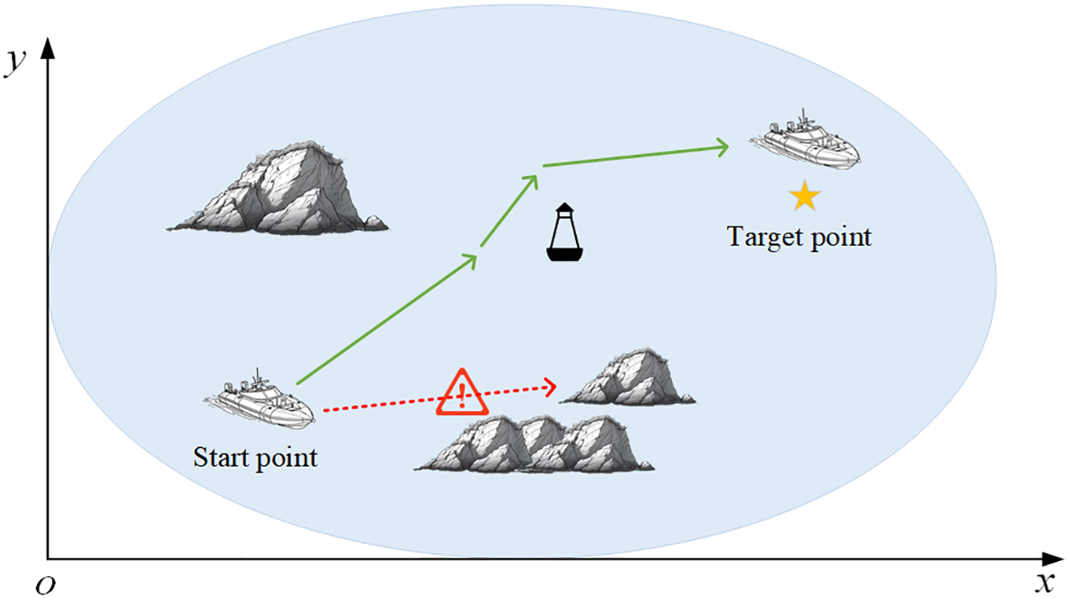
Figure 1. USV path planning.

2.1 Markov decision process

In an MDP, a USV can be abstracted into an agent with the corresponding attributes of the USV. MDP can be expressed as a four-tuple $M=[S,A,P,R]$,where S is the finite set of states in the environment, $s_t$is the state at the time t, A presents the set of all actions that the agent can execute, $a_t$presents the action performed by the agent at the time t, P presents the state transfer probability, averaging the probability that the state $s_t$moves to the next state $s_{t+1}$, and R is the reward function. Based on the observed current state $s_t$, the agent chooses the action $a_t$to execute and enters the next state $s_{t+1}$, and the environment gives the agent a reward $r_{t+1}$when the agent enters the state $s_{t+1}$. Figure 2 illustrates the MDP that models the interaction between the agent and the environment.

Figure 2

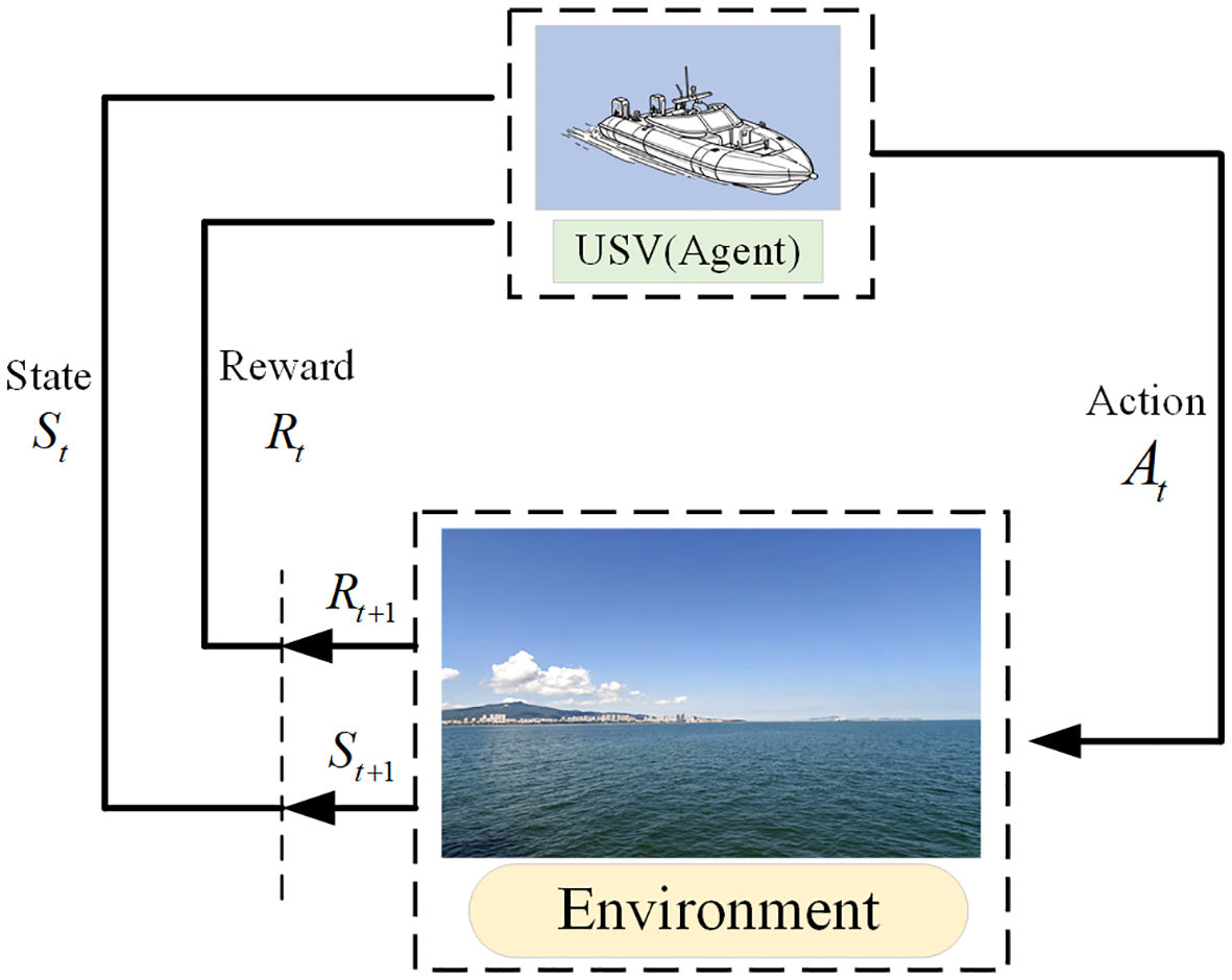
Figure 2. USV Markov decision process.

The agent aims to acquire the optimal policy through the learning process. The optimal policy enables the agent to maximize the return for every episode. For each episode, the return $G_t$is calculated as the discounted sum of rewards $r_t$. The return $G_t$ can be expressed as Equation 1:

$\begin{array}{ll}{G}_t=r_{t+1}+\gamma r_{t+2}+{\gamma }^2{r}_{t+3}+···={\displaystyle \sum _{k=0}^{\infty }{\gamma }^k{r}_{t+k+1}}\gamma \in [0,1]& (1)\end{array}$

where $r_t$ is the reward that the agent obtains at step $t$. $\gamma$ is the discount factor, which represents the relationship between the immediate reward and the long-term reward.

The state value function is the value of state s in the environment under policy $\pi$. State value function can be expressed as Equation 2:

$\begin{array}{ll}{V}^{\pi }(s)=E_{\pi }[G_t|S_t=s]=E_{\pi }[{\displaystyle \sum _{k=0}^{\infty }{\gamma }^k{r}_{t+k+1}}|S_t=s]& (2)\end{array}$

Similarly, action value function $Q_{\pi }(s,a)$ is the value of taking action a in state s under policy $\pi$. The action value function $Q_{\pi }(s,a)$ presents the expected cumulative reward when USV takes action a in state s under policy $\pi$. The action value function $Q_{\pi }(s,a)$ can be expressed as Equation 3:

$\begin{array}{ll}{Q}_{\pi }(s,a)=E_{\pi }[G_t|S_t=s,A_t=a]=E_{\pi }[{\displaystyle \sum _{k=0}^{\infty }{\gamma }^k{r}_{t+k+1}}|S_t=s,A_t=a]& (3)\end{array}$

The Bellman optimality equation for the state value function and the action value function can be expressed as Equations 4, 5:

$\begin{array}{ll}{V}^{*}(s)=\underset{a}{\max }E[r_{t+1}+\gamma V^{*}(s_{t+1})|s_t=s,a_t=a]& (4)\end{array}$

$\begin{array}{ll}{Q}^{*}(s,a)=E[r_{t+1}+\gamma \underset{a}{\max }{Q}^{*}(s_{t+1},a_{t+1})|s_t=s,a_t=a]& (5)\end{array}$

Where $V^{*}$ and $Q^{*}$ present the maximum state value and action value of the state s under the optimal policy ${\pi }^{*}$. The optimal policy can be determined by ${\pi }^{\ast }(s)=\arg \max Q^{\ast }(s,a)$.

2.2 Deep Q-network

In this section, the DQN algorithm is used to solve the USV path planning problem. The DQN algorithm, as a representative deep reinforcement learning method, effectively combines Q-learning with deep learning. This combination enables the DQN algorithm to obtain the optimal policy in a high dimensional state space without relying on prior information about the environment (Mnih et al., 2015). Therefore, the DQN algorithm can enable agents to generate optimal paths under conditions of limited external environment information.

The neural network is used to fit the Q-table in the DQN algorithm, as shown in Equation 6. During the training process, the agent constantly interacts with the environment to generate experience data. Specifically, the agent uses the Q-evaluation network to get the next action a at the state s, and executes the action according to a certain action selection probability $ϵ$. The commonly used action selection probability function is $ϵ\text{-greedy}$,which can be expressed as Equation 6:

$\begin{array}{ll}\pi (a|s)=\{\begin{array}{cc}1-\frac{\epsilon }{\left|A(s)\right|}(\left|A(s)\right|-1),& \text{for the greedy action}\\ \frac{\epsilon }{\left|A(s)\right|},& \text{for the other }\left|A(s)\right|-1\text{ actions}\end{array}& (6)\end{array}$

Where $\pi (a|s)$ is the policy that agent will take at the state s, and $\left|A(s)\right|$ is the number of actions associated with s

After executing the action, the agent enters into the next state $s^{\prime }$ while obtaining a reward r. Through this process, the experience data of the interaction between the agent and the environment are stored in the form of tuples $(s,a,r,s^{\prime })$. Then, the experience caches in the replay buffer.

The difference between the Q-evaluation network and the Q-target network is the way to use empirical data and update the network. Specifically, the Q-evaluation network directly derives state values based on the current state s, while the Q-target network calculates state values based on the next state $s^{\prime }$ and the reward r earned. By calculating the error between the Q-evaluation and Q-target networks, the parameters of the Q-evaluation network can be updated. While for the parameters in the Q-target network, the network parameters of the Q-evaluation are directly copied to the Q-target network at a certain time interval. The calculation of the Q-target network can be expressed by the Equation 7:

$\begin{array}{ll}{Q}_{\text{target}}=r+\gamma \underset{a}{\max }Q(s^{\prime },a;{\theta }^{-})& (7)\end{array}$

where $\underset{a^{\prime }}{\max }Q(s^{\prime },a^{\prime };{\theta }^{-})$ is the maximum value of the Q-evaluation network output, $a^{\prime }$ is the action taken by the agent at the state $s^{\prime }$, and ${\theta }^{-}$ is the Q-target network’s parameter.

The loss function $L(\theta )$ is defined by the mean square deviation between two action values predicted by Q-evaluation network and Q-target network, which can be expressed as Equation 8:

$\begin{array}{ll}L(\theta )=E[{(Q_{\text{target}}-Q_{\text{eval}}(s,a;\theta ))}^2]& (8)\end{array}$

where $Q_{\text{eval}}(s,a;\theta )$ denotes the output of the Q-evaluation network and $\theta$ denotes the parameters of the network.

2.3 Artificial potential field

The Artificial Potential Field (APF) algorithm first appeared in a paper published by Oussama Khatib in 1985 (Khatib, 1985). The APF algorithm assumes that there exists a gravitational force on the target point and a repulsive force on the obstacle point. The gravitation force can attract the agent to go to the target point, while repulsive force makes the agent stay away from obstacles and avoid colliding with obstacles. The agent is subjected to the field force at every point on the map. The field force is equal to the sum of the gravitational and repulsive forces at that point.

The gravitational field can be expressed as Equation 9:

$\begin{array}{ll}{U}_{\text{att}}(h)=\frac{1}{2}\xi {\rho }^2(h,h_{\text{goal}})& (9)\end{array}$

where $\xi$ is the gravitational coefficient, $\rho (h,h_{\text{goal}})$ is the distance between the location h of the agent and the location $h_{\text{goal}}$ of the target point.

The gravitational force exerted by the target point on the agent can be derived by calculating the gradient of the gravitational field. The gravitational force can be expressed as Equation 10:

$\begin{array}{ll}{F}_{\text{att}}(h)=-\xi \rho (h,h_{\text{goal}})& (10)\end{array}$

In order to avoid the collision between the agent and obstacles, the repulsive field exhibits a different property from the gravitational field. For the repulsive field, the closer the agent is to the obstacle, the larger the repulsive field becomes. The repulsive field can be expressed as Equation 11:

$\begin{array}{ll}{U}_{res}(h)=\{\begin{array}{cc}\frac{1}{2}k{(\frac{1}{\rho (h,h_{obi})}-\frac{1}{{\rho }_{obi}})}^2& 0<\rho (h,h_{obi})\le {\rho }_{obi}\\ 0& \rho (h,h_{obi})>{\rho }_{obi}\end{array}& (11)\end{array}$

where k is the repulsion coefficient, $\rho (h,h_{obi})$ is the distance between the location h of the agent and the location $h_{obi}$ of the ith obstacle $obi$. ${\rho }_{obi}$ is the maximum repulsive force range of the obstacle $obi$. When the agent leaves the repulsive force range of the obstacle, the agent is no longer subject to the repulsive force of this obstacle.

The repulsive force generated by obstacles can be derives by calculating the gradient of the repulsive force field. The repulsive force can be expressed as Equation 12:

$\begin{array}{ll}{F}_{res}(h)=\{\begin{array}{cc}k(\frac{1}{\rho (h,h_{obi})}-\frac{1}{{\rho }_{obi}})\frac{\nabla \rho (h,h_{obi})}{\rho {(h,h_{obi})}^2}& 0<\rho (h,h_{obi})\le {\rho }_{obi}\\ 0& \rho (h,h_{obi})>{\rho }_{obi}\end{array}& (12)\end{array}$

The combined force acting on the agent is a superposition of gravitational and repulsive forces, so the combined force acting on the agent can be written as Equation 13:

$\begin{array}{ll}F(h)=F_{\text{att}}(h)+F_{\text{res}}(h)& (13)\end{array}$

The gravitational force generated by the target point will make the agent move toward the target point, and the repulsive force generated by the obstacle will prevent the agent from approaching the obstacle. Through the superposition of gravitational force and repulsive force, the agent can avoid the obstacle and reach the target location.

However, as shown in Equation 13, the agent is ultimately subject to the combined force of the gravitational force and the repulsive force. In some special cases, there may be a situation where the repulsive force is balanced with the gravitational force, as shown in Figure 3. In addition, when obstacles are gathered at the annex of the target point, it is possible that the combined repulsive force of the obstacles will be greater than the gravitational force at the target location, and thus, the target location will no longer be the point with the smallest potential field in the whole map, resulting in the agent not being able to reach the target location.

Figure 3

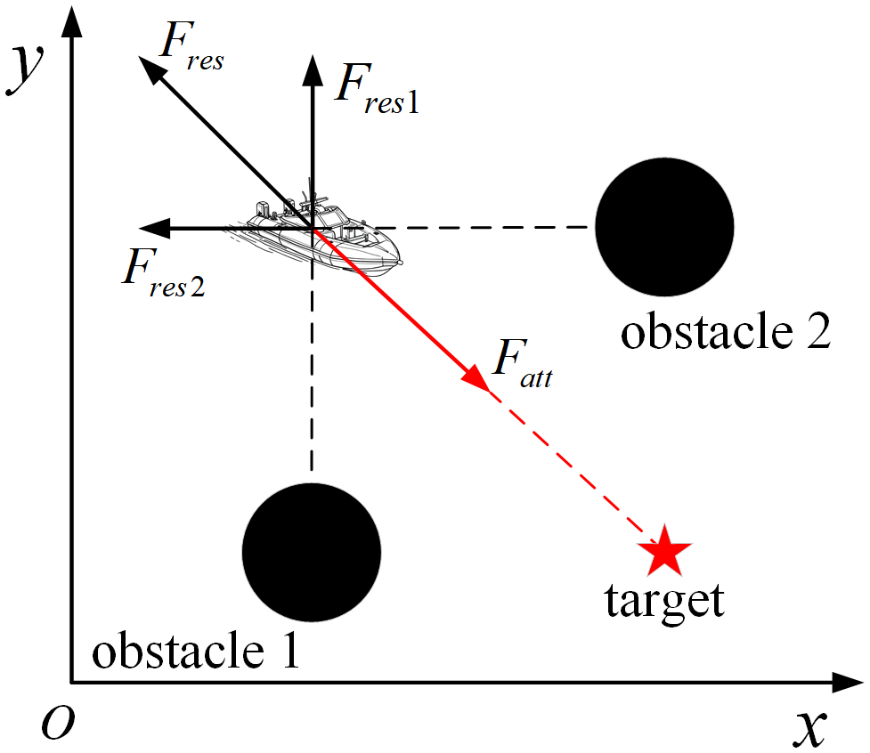
Figure 3. Gravitational force and repulsive force balance.

3 APF-RADQN-based path planning algorithm

In this section, a MDP model of the USV is first established. The MDP model primarily consists of the state space, the action space, and the reward function. Secondly, an APF-RADQN framework based on improved network error calculation is proposed, which is used to solve the MDP model of USV path planning. Then, the optimal path is obtained by the path smoothing method.

3.1 MDP model for USV route planning

1. State space: Grid map-based metric modeling is the mainstream environmental map building method (Koval et al., 2022; Wu et al., 2022). Meanwhile, unlike UAVs that can float or dive, USVs only move on the surface of the water. In that case, USVs are mainly concerned with the environmental state information of the plane of movement where they are located. Therefore, the three-dimensional spatial environment can be converted into a two-dimensional planar environment, as shown in Figure 4. The navigation environment of the USV is set as a two-dimensional grid map environment of 60m*60m. According to the distribution of obstacles in the environment, the obstacles are represented by black grids, and the area that can be freely passed is represented by white grids. Each of the grid is a square with a width of 1 meter. In particular, in order to facilitate the construction of the simulation map environment and to ensure the safe navigation of the USV, obstacles that do not occupy a complete grid in actuality are regarded as occupying a complete grid in the gridded map. Additionally, the grid map-based environment is determined in this study, which meaning when the agent takes the action a at state $s_t$, then the next state $s_{t+1}$ of the agent is determined. Thus, the state transfer probability P can be expressed as $P(s_{t+1}|s_t,a)=1$.

Figure 4

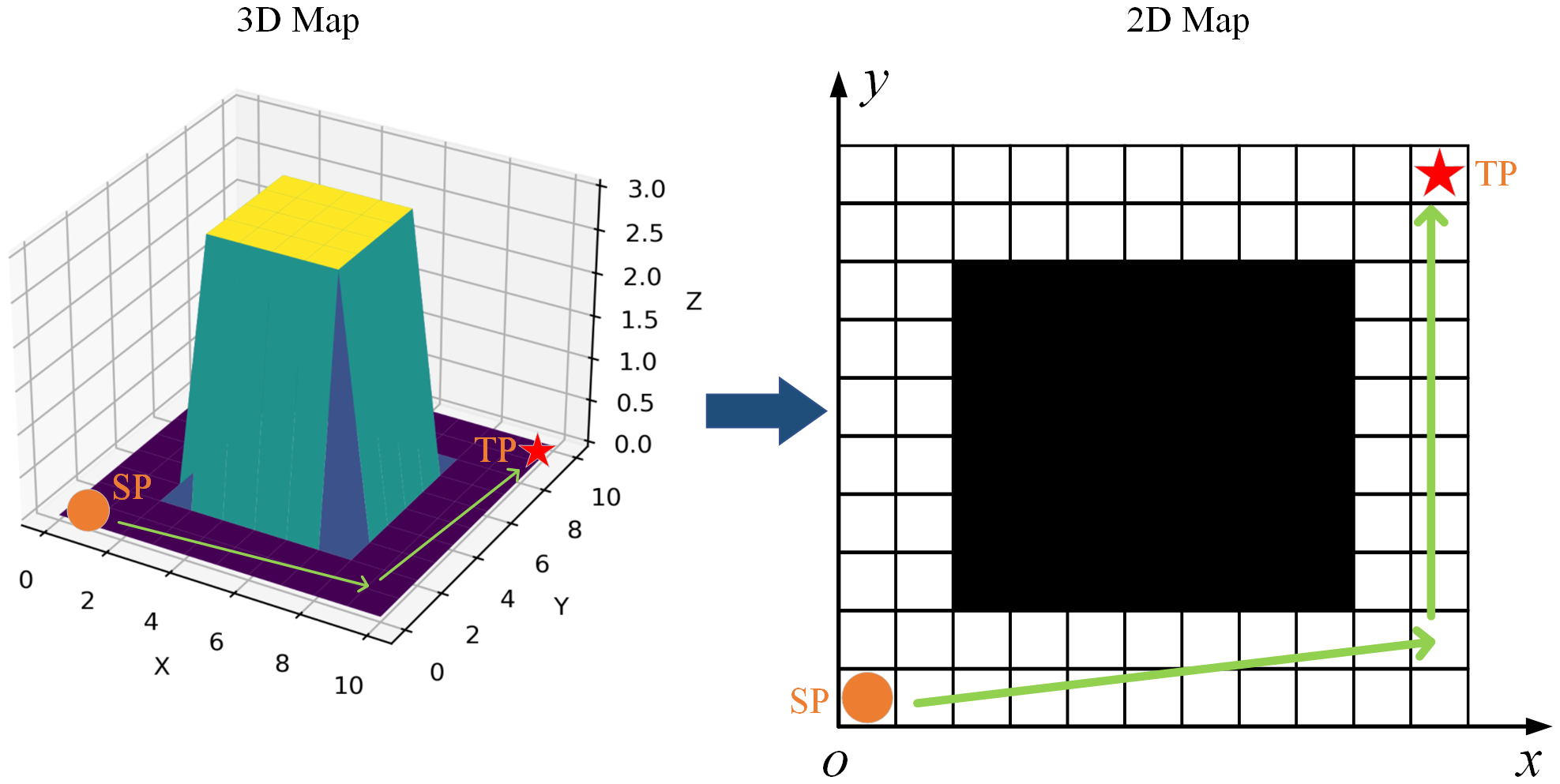
Figure 4. Conversion of a 3D spatial environment into a 2D planar environment.

The Euclidean distance is used to measure the distance between the USV and the target point when calculating the path length. So, the coordinate position $(x,y)$ of the USV and the distance to the target point $D{T}_i$ are introduced into the state space. The state space equation of the USV can be expressed as Equation 14:

$\begin{array}{ll}S=\left[\begin{array}{lll}{x}_1\hfill & y_1\hfill & D{T}_1\hfill \\ x_2\hfill & y_2\hfill & D{T}_2\hfill \\ ⋮\hfill & ⋮\hfill & ⋮\hfill \\ x_t\hfill & y_t\hfill & D{T}_t\hfill \end{array}\right]& (14)\end{array}$

2. Action space: typically, the propulsion, steering and other motion states of a USV are realized by coordinating the thrust of propellers with the deflection angle of its rudder. Although the navigation process of USVs in real environments is continuous, the navigation of USVs within a period of time can be regarded as movement within a grid. Therefore, the navigation process of USVs in real environments can be converted into a series of grid movements of agents in grid maps. Moreover, in order to simplify the USV’s motion model, in the path planning process, it is assumed that the speed of the USV is certain, and at the same time, the USV’s action space is decomposed into 8 directions $A=\{\text{right, down, left, up, lower right},\text{ upper right, lower left},\text{ upper left}\}$, i.e., the action space. The specific action space is shown in Figure 5. Based on the above assumptions, the movement rules of USV in the gridded map environment can be represented as Equation 15:

Figure 5

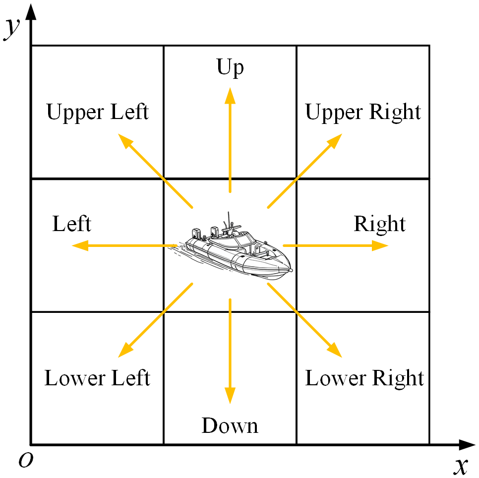
Figure 5. USV action space.

$\begin{array}{ll}\{\begin{array}{l}(x^{\prime },y^{\prime })=(x+\text{grid},y)\hfill \\ (x^{\prime },y^{\prime })=(x,y+\text{grid})\hfill \\ (x^{\prime },y^{\prime })=(x-\text{grid},y)\hfill \\ (x^{\prime },y^{\prime })=(x,y-\text{grid})\hfill \\ (x^{\prime },y^{\prime })=(x+\text{grid},y+\text{grid})\hfill \\ (x^{\prime },y^{\prime })=(x+\text{grid},y-\text{grid})\hfill \\ (x^{\prime },y^{\prime })=(x-\text{grid},y+\text{grid})\hfill \\ (x^{\prime },y^{\prime })=(x-\text{grid},y-\text{grid})\hfill \end{array}& (15)\end{array}$

where $(x,y)$ denotes the current position state of the USV, $(x^{\prime },y^{\prime })$ denotes the next position state of the USV, and $grid$ denotes the width of the unit grid. It is important to emphasize that each action performed by the USV in the gridded map only allows it to move to an adjacent grid.

3. Reward Function: In the MDP framework, the reward function is used to evaluate the value of an action a taken by the agent. In previous studies, an agent receives a positive reward when it reaches the target location and a negative reward for entering a forbidden zone such as an obstacle or a boundary. However, under this reward distribution, all other states receive zero reward, which causes the problem of reward sparsity in reinforcement learning. This problem leads to difficulties for reinforcement learning algorithms to find feasible solutions. Therefore, this paper proposes a composite reward function $R_t$. The proposed reward function makes it possible to receive a reward for agent at all state during the training process. The composite reward function can be expressed as Equation 16:

$\begin{array}{ll}{R}_t=r_{\tau 1}+r_{\tau 2}+r_{\tau 3}+r_{\tau 4}& (16)\end{array}$

where $r_{\tau 1}$ is the target reward function, $r_{\tau 2}$ is the obstacle reward function, $r_{\tau 3}$ is the boundary reward function, and $r_{\tau 4}$ is the potential field reward function.

Specifically, $r_{\tau 1}$ is usually set as a positive reward to motivate the agent to reach the target position, and the target reward function can be calculated by the Equation 17:

$\begin{array}{ll}{r}_{\tau 1}=\{\begin{array}{cc}{\lambda }_1,& DT\le \frac{\sqrt{2}}{2}\text{grid}\\ 0,& \text{otherwise}\end{array}& (17)\end{array}$

Where ${\lambda }_1$ is a positive reward value, which is available when the agent enters the target position. To improve the training efficiency of the model, the task is considered completed when the agent reaches a certain range of the target point. For the grid map, the task is considered completed when the agent enters the grid where the target point is located.

where DT is the Euclidean distance from the agent to the target point, which can be expressed by Equation 18:

$\begin{array}{ll}D{T}_i=\sqrt{{(x_i-x_{\text{target}})}^2+{(y_i-y_{\text{target}})}^2}& (18)\end{array}$

During the navigation process, agent should avoid the collision with obstacles in the environment. In grid-based map, the agent should not drive into the grids labeled as obstacles on the map. The obstacle reward function $r_{\tau 2}$ can effectively avoid the agent from colliding with obstacles in the grided-based movement, and its expression as Equation 19:

$\begin{array}{ll}{r}_{\tau 2}=\{\begin{array}{cc}{\lambda }_2,& \text{OD}<R_s\\ 0,& \text{OD}\ge R_s\end{array}& (19)\end{array}$

where ${\lambda }_2$ is a negative value indicating the penalty for the agent to enter the range of an obstacle, OD is the Euclidean distance from the agent to the closest obstacle to the agent, and $R_s$ is the safe distance that the agent should maintain from the obstacle.

Boundary rewards are used to limit the area of activity of an agent. Ensure that the agent operates within a predefined range of the environment. Boundary rewards can be defined as Equation 20:

$\begin{array}{ll}{r}_{\tau 3}=\{\begin{array}{cc}{\lambda }_3,& \left(\begin{array}{c}x>\max (x\text{) or }x<\min (x)\\ y>\max (y\text{) or }y<\min (y)\end{array}\right)\\ 0,& \text{otherwise}\end{array}& (20)\end{array}$

where reward ${\lambda }_3$ is a negative value, $\max (x)$ and $\min (x)$ are the maximum and minimum horizontal coordinates of the environmental map, $\max (y)$ and $\min (y)$ are the maximum and minimum vertical coordinates of the environmental map.

When the agent explores the environment, if rewards are only set at key points that directly affect the success or failure of the task, such as target points, boundaries and obstacles, while rewards are zero at other relatively unimportant locations, it will lead to slower convergence of the algorithm, or even ultimately fail to obtain a valid path. Therefore, continuous rewards are needed to provide guidance to the agent during its exploration of the environment. The successive rewards should have the ability to guide the agent to the target location while avoiding factors such as obstacles and boundaries. As shown in Equations 10, 12 and 13, the APF method is characterized by a continuous distribution of potential field forces in the map environment. Specifically, potential field forces point to the target point at locations away from obstacles, and point in the direction away from obstacles near obstacles. The motion direction of the agent in the environment is shown in Equation 15. According to the motion direction of the agent, the motion of the agent can be rewritten in the form of vector as Equation 21:

$\begin{array}{ll}\{\begin{array}{l}{\overrightarrow{a}}_{ \text{right}}=(x+\text{grid},y)=(1,0)\hfill \\ {\overrightarrow{a}}_{ \text{down}}=(x,y+\text{grid})=(0,1)\hfill \\ {\overrightarrow{a}}_{ \text{left}}=(x-\text{grid},y)=(-1,0)\hfill \\ {\overrightarrow{a}}_{ \text{up}}=(x,y-\text{grid})=(0,-1)\hfill \\ {\overrightarrow{a}}_{ \text{lower\_right}}=(x+\text{grid},y+\text{grid})=(1,1)\hfill \\ {\overrightarrow{a}}_{ \text{upper\_right}}=(x+\text{grid},y-\text{grid})=(1,-1)\hfill \\ {\overrightarrow{a}}_{ \text{lower\_left}}=(x-\text{grid},y+\text{grid})=(-1,1)\hfill \\ {\overrightarrow{a}}_{ \text{upper\_left}}=(x-\text{grid},y-\text{grid})=(-1,-1)\hfill \end{array}& (21)\end{array}$

Therefore, in this paper, a potential field reward function is proposed in combination with the APF method, the reward function is expressed as Equation 22:

$\begin{array}{ll}{r}_{\tau 4}=\overrightarrow{a_s}·\overrightarrow{F(s)}=\left|\overrightarrow{a_s}\right|\left|\overrightarrow{F(s)}\right|\cos \theta & (22)\end{array}$

where the reward $r_{\tau 4}$ is the dot product of the vector $\overrightarrow{a_s}$ and vector $\overrightarrow{F(s)}$, the vector $\overrightarrow{a_s}$ is the action taken by the agent in the state $s$, vector $\overrightarrow{F(s)}$ is the potential force on the agent in the state $s$, $\cos \theta$ is the cosine of the angle between two vectors, when $0<\left|\theta \right|<\frac{\pi }{2}$, the reward $r_{\tau 4}$ is positive, when $\frac{\pi }{2}<\left|\theta \right|<\pi$, the reward is negative. Figure 6 shows the reward $r_{\tau 4}$ distribution. In the situation of the Figure 6, supposing the APF force is the unit, the angle $\theta$ is $\frac{\pi }{6}$, and the action vectors are defined by the Equation 21.

Figure 6

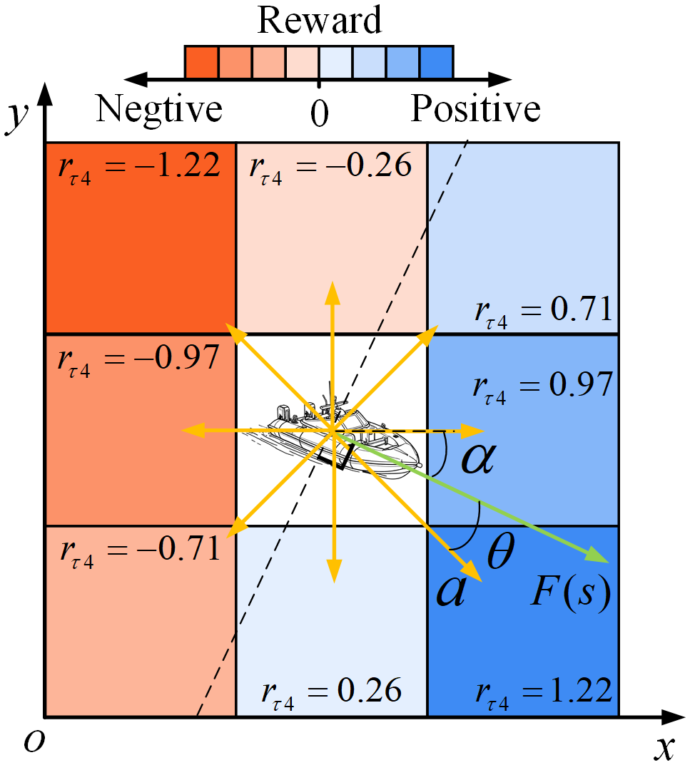
Figure 6. Distribution of rewards.

Equation 22 demonstrates the relationship between action and reward: the reward increases when the agent’s action direction aligns with the artificial potential field; The reward decreases as the action deviates from the potential field’s guidance; the reward transitions to negative values if the agent’s motion opposes the potential field direction. Through the guidance of the artificial potential field, the agent can obtain a feasible path more quickly.

3.2 APF-RADQN framework for USVs

1. Deep Neural Networks: The DQN algorithm uses deep neural networks (DNN) to approximate the action value function (Hadi et al., 2022). In addition, both the Q-evaluation network and the Q-target network use the same DNN network structure. The DNN structure consists of an input layer, several hidden layers and an output layer. The network parameters are trained through supervised learning. The input to the neural network consists of two parts: 1) the environmental information collected by the sensors and 2) the positional information of the USV. These inputs are processed through the fully connected layer and finally the computed results are output to the output layer. The output layer gives the Q-values of all executable actions and finally selects the action with the largest Q-value as the output of the network. In this network structure, the rectified liner unit (ReLu) function is used as an activation function between the input layer and each hidden layer.

The ReLu function can be expressed as Equation 23:

$\begin{array}{ll}\sigma (\xi )=\{\begin{array}{cc}\xi ,& \xi >0\\ 0,& \xi \le 0\end{array}& (23)\end{array}$

To improve the learning efficiency of the DNN, the adaptive moment estimation (Adam) algorithm is used to optimize the learning rate. The Adam optimizer enables adaptive updating of the learning rate (Chen et al., 2024). Meanwhile, Adam optimizer introduces a dynamic term to improve the stochastic gradient descent of the neural network. Subsequently, the current network is optimized through integration with the gradient explosion prevention method, thereby enhancing the predictive capability of the DQN algorithm.

2. Network reward-averaging strategy: as a key factor in reinforcement learning, rewards influence the learning efficiency and eventual convergence of the algorithm (De Moor et al., 2022). Agents continuously acquire rewards in their interactions with the environment and store these rewards in the experience replay buffer. During the network training process, these reward-contained experiences are also continuously used as training inputs in the process of optimizing the deep network. Recent studies show that optimizing the reward calculation in the DRL training process can speed up learning and improve the convergence of the network. (Naik et al., 2019; Sutton and Barto, 2020). To reduce the variance of the reward signal, the reward in each training step subtracts from the average reward. In the DQN algorithm, the network is updated by computing the temporal difference (TD) error between the Q-evaluation and Q-target values. Q-target value is calculated by reward and discounted action value. Therefore, when calculating the Q-target value and TD error, the reward obtained from the reward-averaging strategy can replace the original reward received from the experience. The Q-target network and the loss function, Equations 7, 8 can be rewritten as Equations 24, 25:

$\begin{array}{ll}{Q^{\prime }}_{\text{target}}=r-rm+\gamma \underset{a}{\max }Q(s^{\prime },a;{\theta }^{-})& (24)\end{array}$

$\begin{array}{ll}L(\theta )=E({({Q^{\prime }}_{\text{target}}-Q_{\text{eval}})}^2)& (25)\end{array}$

where ${Q^{\prime }}_{\text{target}}$ is the output of the target network subtracting the mean value of the rewards, and $rm$ is the mean value of the historical rewards, which can be expressed by the Equation 26:

$\begin{array}{ll}r{m}_{t+1}=r{m}_t+\eta \text{mean}(\delta )& (26)\end{array}$

where $\eta$ is the learning coefficient of the reward mean, $\delta$ is the difference between the ${Q^{\prime }}_{\text{target}}$ value and the $Q_{\text{eval}}$ value, $r$ is the total reward corresponding to the training step.

3. Path smoothing: The output of the APF-RADQN algorithm is discrete, while the navigation of the USV is continuous. The points generated by the algorithm need to be smoothed to make the paths closer to the actual USV navigation. Bezier curve has the advantages of high controllability, good path smoothing, and less occupied computation (Song et al., 2021). Bezier curve is widely used in curve smoothing related graphical processing work. Therefore, the introduction of Bezier curve into the framework of APF-RADQN algorithm can realize the end-to-end smoothing path planning. the computational expressions of Bezier curve from the first order to the third order are as Equation 27:

$\begin{array}{ll}{c}_i^k=\{\begin{array}{cc}{c}_i^0,& i=0,1,2,\dots ,n-k\\ (1-t)c_i^{k-1}+t{c}_{i+1}^{k-1},& i=0,1,2,\dots ,n-k\end{array}& (27)\end{array}$

where $c_i^0$ represents the ith initial control point, $c_i^k$ represents the ith K-order control point (k=1, 2, …, n), and $t$ represents the scale factor.

According to Equation 27, the formula for n-order control points always contains two n-1 order control points, thus the formula for n-order control points can be finally calculated from the initial control points. Second-order Bezier curves ensure smoothness of paths and have faster computation speeds than higher-order Bezier curves. Therefore, multiple second-order Bezier curves are used in series for smoothing the path as Equation 28:

$\begin{array}{ll}\begin{array}{cc}B(t)=(1-t^2)c_i^0+2(1-t)c_{i+1}^0+t^2{c}_{i+2}^0,& t\in [0,1]\end{array}& (28)\end{array}$

where $c_i^0$, $c_{i+1}^0$ and $c_{i+2}^0$ denote three consecutive initialization control points.

4. USV path planning process: in summary, the flowchart of the APF-RADQN algorithm applied to USV path planning is shown in Figure 7. The pseudocode of the algorithm is shown in Algorithm 1 . The flow of Code 1 is depicted roughly as follows.

Figure 7

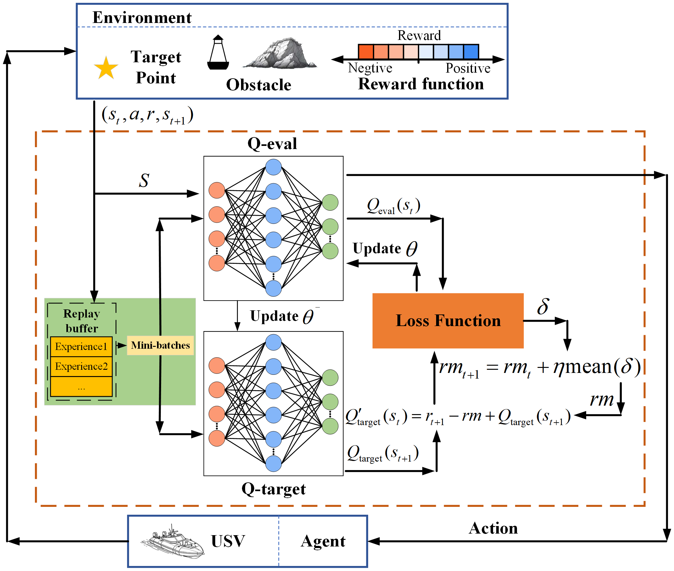
Figure 7. Algorithm flow chart.

Step 1: First, set the training parameters, mainly including state space, action space, reward, initial learning rate, etc. (line 1); second, establish Q-evaluation neural network and Q-target neural network; third, randomly initialize the parameters $\theta$ and ${\theta }^{-}$, and make $\theta ={\theta }^{-}$ (line 2).

Step 2: USV explores the environment. The environment is first reset before the start of each episode (line 5). During the exploration process, the current state inputs to the Q-evaluation network and the response action is calculated. The resulting action is executed according to the $\text{ϵ-greedy}$ policy. The USV interacts with the environment to receive rewards r and the next state s (lines 7-10).

Step 3: Update process of Q-evaluation and Q-target network. First, the sampled data collected during exploration are saved in the experience replay buffer, and then a batch of experience data are randomly selected from the experience replay buffer for updating the current network (lines 11-15). The Q-target network and the Q-evaluation network are computed using empirical data, and then the error between the networks is computed and updated rm. Second, the loss function is computed and the parameters of the Q-evaluation network are updated based on the backpropagation of the gradient of the neural network. Third, update the parameters of the Q-target network (lines 17-18).

Step 4: After multiple rounds of training, save the final training parameters of the network and the USV output optimal path (lines 21-23).

Algorithm 1. APF-RADQN Algorithm.

4 Experimental simulation

In order to verify the feasibility of the proposed APF-RADQN algorithm, the simulation model of the proposed APF-RADQN algorithm and the other three path planning algorithms is established in PyCharm platform, and three 60*60 dimension grid-based map environments are established for the visualization of the results. The hyperparameter configurations of the APF-RADQN algorithm are summarized in Table 1. The operating system used for testing algorithms is Windows 11. The hardware configuration: CPU is Intel i9 13900hx, GPU is Nvidia RTX 4060, 8G video memory. The proposed APF-RADQN algorithm is compared with the baseline algorithm in the same three unknown obstacle environments to verify the effectiveness and superiority of the APF-RADQN algorithm.

Table 1

Table 1. Algorithm parameters.

4.1 Baseline algorithms

Comparison algorithms are described as follows:

1. APF: The APF algorithm quickly and flexibly plans an effective path by calculating the gradient of the potential field in the environment. The path trajectory can maintain a safe distance from obstacles.

2. A*: The A* algorithm accurately guides the robot to explore the environment by utilizing the principles of breadth-first search and best-first search. These search methods ensure the shortest path could be found in the limited state space.

3. DQN: The DQN algorithm obtains empirical data through the agent’s continuous interaction with the environment, uses the empirical data to train the deep neural network, and finally obtains the optimal path through the neural network. Meanwhile, the state space, action space and reward function are the same of the proposed APF-RADQN algorithm.

Based on the advantages of APF algorithm, A* algorithm and DQN algorithm, the performance of different algorithms for planning path results in three aspects: 1) path length; 2) path smoothness; and 3) algorithmic inference time (IT) are evaluated to evaluate the superiority and effectiveness of the proposed APF-RADQN algorithm.

In addition, the computational complexity of all the compared algorithms is shown below. The computational complexity of the proposed APF-RADQN algorithm is $O(EP*N)$, which is the same as that of the conventional DQN algorithm, where N is the step number in each episode and EP is the number of episode, The computational complexity of the A* algorithm is $O(N_1\log N_1)$,where $N_1$ denotes the number of nodes. The computational complexity of the APF algorithm is $O(N_2*M)$, where $N_2$ denotes the number of iterations and M denotes the number of obstacles.

4.2 Environmental simulation experiments and results

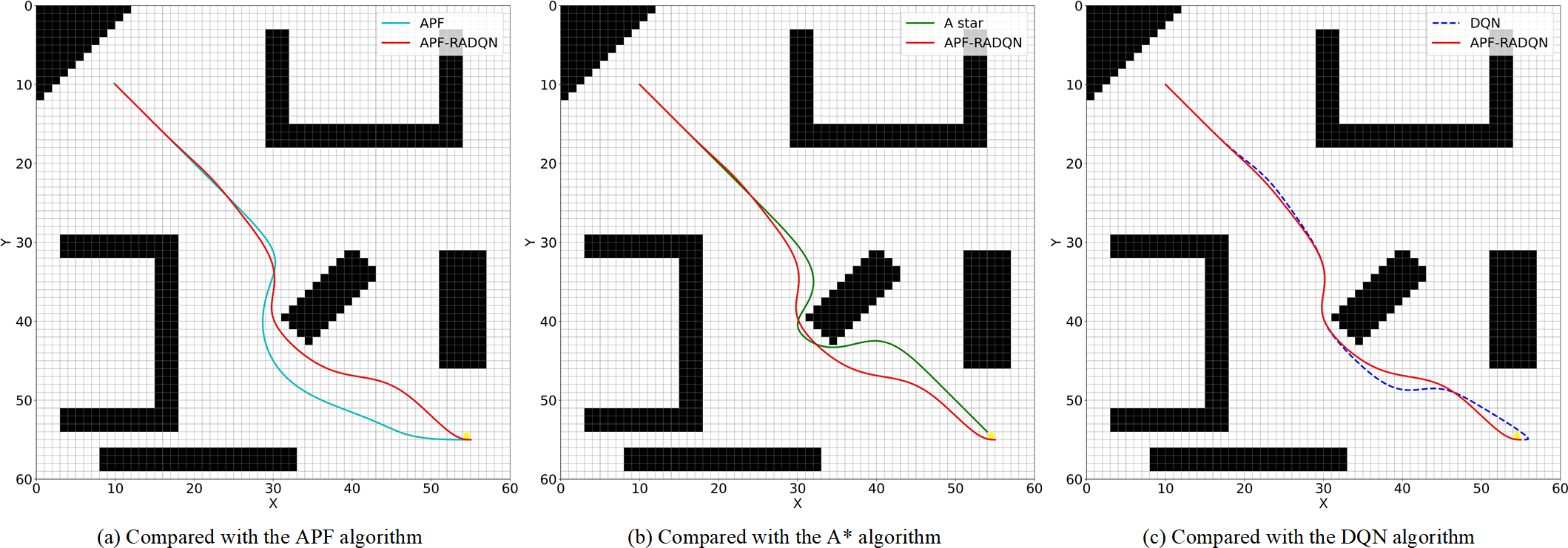
In this paper, three environments A, B, and C with different terrain features and obstacle densities are designed and tested. USV didn’t learn three environments in advance to evaluate the performance of the proposed APF-RADQN algorithms and compare algorithms. First, three key performance indicators (KPIs) are established to evaluate the performance of various path planning algorithms. KPIs include average path length, average number of path corners, and algorithm inference time. The planned paths of these 4 algorithms in 3 different simulation environments are given in Figures 8–10, and the KPI values are given in Table 2.

Figure 8

Figure 8. Planned path in environment A. (a) Compared with the APF algorithm, (b) Compared with the A* algorithm, (c) Compared with the DQN algorithm.

Figure 9

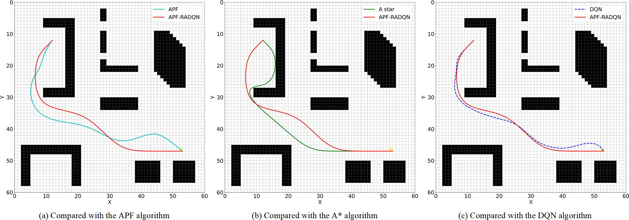
Figure 9. Planned path in environment B. (a) Compared with the APF algorithm, (b) Compared with the A* algorithm, (c) Compared with the DQN algorithm.

Figure 10

Figure 10. Planned path in environment C. (a) Compared with the APF algorithm, (b) Compared with the A* algorithm, (c) Compared with the DQN algorithm.

Table 2

Table 2. Algorithmic KPIs.

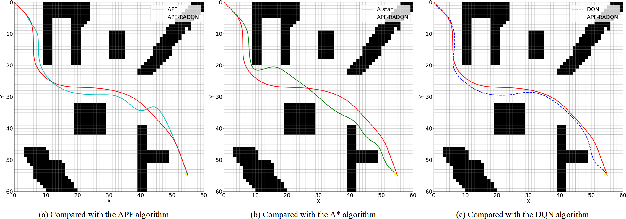
4.2.1 Path analyses of environment A

In Figure 8, the distance between SP and TP is relatively long in environment A. Trap areas do not easily impede the agent. All four algorithms can find collision-free routes. However, there are some differences in details, where the APF algorithm requires the most steps and the A* algorithm has the greatest risk of collision.

In the APF algorithm, shown in Figure 8a, the target point continuously attracts the agent, while the agent experiences a repulsive force only near obstacles. This mechanism explains why the path generated by the APF algorithm is closer to obstacles than the APF-RADQN generated one during initial navigation phases. With the approaching of the target point, the gravitation force is declared. Thus, the agent in the APF algorithm stays away from obstacles gradually. The comparison with the A* algorithm is shown in Figure 8b. Because the A* algorithm is only searching nearby points at each point, the path planned by the A* algorithm can’t maintain enough safety distance to obstacles when the agent passes through obstacles, as shown in Figure 8c. The two paths generated by the DQN and APF-RADQN algorithms are similar in nature. However, the APF-RADQN algorithm can generate a smoother path.

4.2.2 Path analyses of environment B

In Figure 9, the distance between SP and TP is relatively short in environment B. Trap areas do not easily impede the agent. The obstacles in the upper left map are distributed symmetrically. In this environment, all four algorithms can generate the collision-free path to reach the target point, while the APF algorithm generates the longest path, and the A* algorithm has the worst smoothness.

The symmetrical zone makes the APF algorithm set a much broader repulsive force range than usual in case of falling into zero potential energy points. But these parameters setting leads to the longest path in this environment, as shown in Figure 9a. The other three algorithms have a similar beginning path, but the A* algorithm’s planned path is quite near obstacles because of its algorithm searching method (Figure 9b), and the DQN algorithm generated some unnecessary turns near the target point (Figure 9c).

4.2.3 Path analyses of environment C

A more complex environment than the previous two maps is shown in Figure 10. The distance between SP and TP is relatively short in environment C. The obstacles around the SP are formed as a trap that easily impedes the agent. In this environment, all four algorithms can generate a collision-free path to reach the target point. However, the A* algorithm fell into the trap and had the longest path.

The agent’s movements at the start need to move in the opposite direction to the target point. This detour examines the interface ability of all four algorithms. As shown in Figure 10a, the APF algorithm can find a way to get out of the initial obstacle because of the combined force. However, multiple obstacles complicate the potential field, resulting in a lot of meaningless turns in the path. Figure 10b shows the dilemma of the A* algorithm at the early stage. Due to the research method of the A* algorithm, the agent cannot foresee the block between the target point and itself. This disadvantage makes the agent get into the trap at the very beginning. Both the DQN algorithm and the APF-RADQN algorithm show outstanding interface ability in Figure 10c. However, the DQN algorithm is still taking more turns than the APF-RADQN algorithm.

4.2.4 Convergence analyses

Figure 11 shows the training return curves of the DQN and APF-RADQN algorithms in three different environments. The action-valued network of the agent has not been sufficiently trained in the early stage of training, and the derived strategies are not reasonable enough, so the return curves fluctuate greatly. Subsequently, the USV trains the neural network using the empirical knowledge gained from exploring the environment, then the output of the neural network is gradually close to the real value, and finally, a more reasonable strategy is obtained, and the reward curves are stabilized. Since the APF-RADQN algorithm proposed introduces reward averaging to improve the network error, fully utilizes the rewards from historical experience, and balances the error brought by accidental exploration, the return curve can converge faster in the early stage of training. As the complexity of the environment increases, both DQN and APF-RADQN need more exploration and training to learn the optimal strategy and achieve return curve stabilization. Although the DQN algorithm is able to achieve return curve stabilization after a period of continuous learning, the overestimation of the Q-value leads to slower convergence. By comparing the trend of return values of the proposed APF-RADQN and DQN, it can be seen that the number of iterative steps required for the APF-RADQN algorithm to reach stable reward values in three different environments is reduced by about 7.2%, 13.8% and 10.1%, respectively. Compared with the DQN algorithm, the comparison results show that APF-RADQN has higher learning efficiency, global search capability and excellent convergence.

Figure 11

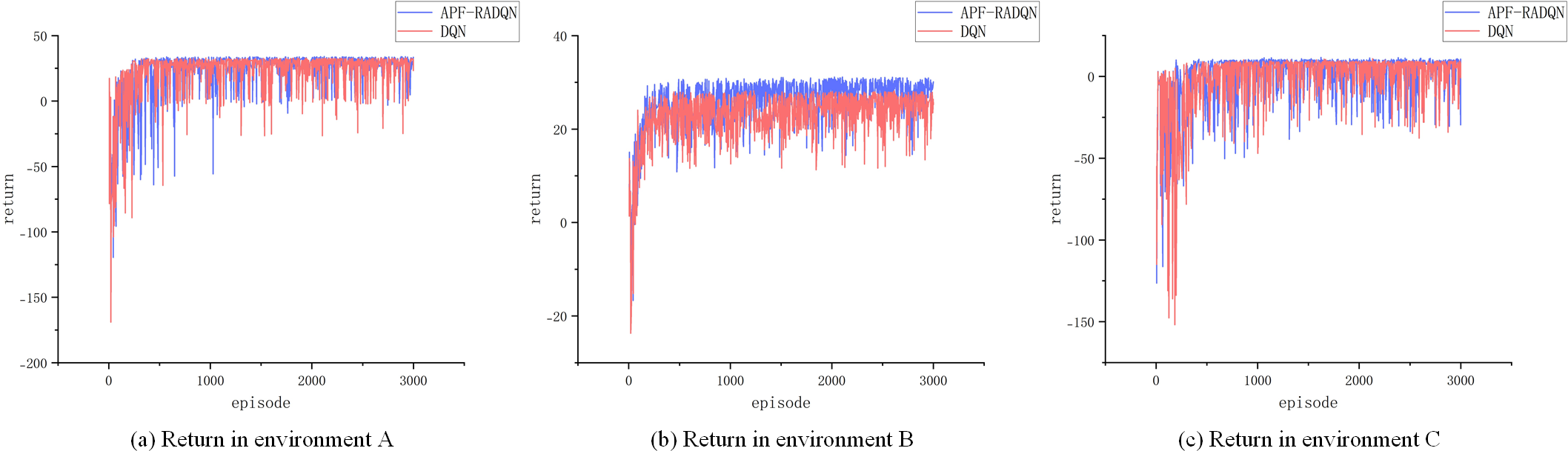
Figure 11. Return curves. (a) Return in environment A, (b) Return in environment B, (c) Return in environment C.

5 Conclusion

In this paper, an algorithm based on the APF-RADQN framework, used for ocean observation missions of USVs, is proposed to address the USV path planning problem. First, a comprehensive reward function combined with the APF algorithm is designed after establishing the USV path planning MDP models, which guides the USV to reach the target area quickly while ensuring that the USV maintains a safe distance from the obstacles. Then, within the framework of the APF-RADQN, a Q-value error calculation method is incorporated, which improves the overall convergence speed and solving capability of the algorithm. In addition, a Bezier curve algorithm is introduced to smooth the discrete movements of the proposed path planning algorithm. Finally, the APF-RADQN-based algorithm is validated in three environments. Compared with DQN, APF algorithm and A* algorithm, the proposed algorithm can find shorter and safer paths and enhance the efficiency of ocean observation missions.

Nevertheless, the proposed algorithm still has some limitations. The algorithm mainly considered the static environments in ocean observation missions, which less consider the dynamic environments and environmental factors such as wind and current. These limitations may influence its usage in complex marine environments. Moreover, the computation burden of the proposed algorithm is quite high, leading to a long interface time. The Future work will focus on improving the algorithm performance in complex ocean observation missions, including using real-time sensor detection to avoid dynamic obstacles, path planning under uncertain environmental perturbations, and the validation of practical algorithms in hardware-closed-loop experiments.

Data availability statement

The raw data supporting the conclusions of this article will be made available by the authors, without undue reservation.

Author contributions

JM: Writing – review & editing, Project administration, Funding acquisition, Methodology. BS: Methodology, Software, Conceptualization, Writing – original draft. BW: Validation, Writing – review & editing, Investigation. CY: Software, Writing – original draft, Methodology. YW: Validation, Writing – review & editing, Funding acquisition. FZ: Writing – review & editing, Formal Analysis, Software. LZ: Data curation, Writing – review & editing, Investigation. JW: Data curation, Writing – review & editing, Investigation. JL: Methodology, Writing – review & editing, Formal Analysis, Conceptualization.

Funding

The author(s) declare that financial support was received for the research and/or publication of this article. This research was supported by the National Natural Science Foundation of China (Grant No. 52175487), the Shandong Province Natural Science Foundation (Grant No. ZR2021ME223), Shandong Offshore Engineering Facility & Material Innovation Entrepreneurship Community (SOFM-IEC) Project (No. GTP-2404), the National Natural Science Foundation of China (Grant No. 52405072).

Conflict of interest

Author CY was employed by Suzhou Tongyuan Software & Control Technology Co., Ltd.

The remaining authors declare that the research was conducted in the absence of any commercial or financial relationships that could be construed as a potential conflict of interest.

Generative AI statement

The author(s) declare that no Generative AI was used in the creation of this manuscript.

Publisher’s note

All claims expressed in this article are solely those of the authors and do not necessarily represent those of their affiliated organizations, or those of the publisher, the editors and the reviewers. Any product that may be evaluated in this article, or claim that may be made by its manufacturer, is not guaranteed or endorsed by the publisher.

References

Al-Kamil S. J. and Szabolcsi R. (2024). Enhancing mobile robot navigation: optimization of trajectories through machine learning techniques for improved path planning efficiency. Mathematics 12, 1787. doi: 10.3390/math12121787

Crossref Full Text | Google Scholar

Antonakis A., Nikolaidis T., and Pilidis P. (2017). Multi-objective climb path optimization for aircraft/engine integration using particle swarm optimization. Appl. Sci. 7, 469. doi: 10.3390/app7050469

Crossref Full Text | Google Scholar

Chen G., Gao Z., Hua M., Shuai B., and Gao Z. (2024). Lane change trajectory prediction considering driving style uncertainty for autonomous vehicles. Mechanical Syst. Signal Process. 206, 110854. doi: 10.1016/j.ymssp.2023.110854

Crossref Full Text | Google Scholar

Chiodi A. M., Zhang C., Cokelet E. D., Yang Q., Mordy C. W., Gentemann C. L., et al. (2021). Exploring the pacific arctic seasonal ice zone with saildrone USVs. Front. Mar. Sci. 8. doi: 10.3389/fmars.2021.640697

Crossref Full Text | Google Scholar

Chu Z., Wang F., Lei T., and Luo C. (2023). Path planning based on deep reinforcement learning for autonomous underwater vehicles under ocean current disturbance. IEEE Trans. Intell. Veh. 8, 108–120. doi: 10.1109/TIV.2022.3153352

Crossref Full Text | Google Scholar

De Moor B. J., Gijsbrechts J., and Boute R. N. (2022). Reward shaping to improve the performance of deep reinforcement learning in perishable inventory management. Eur. J. Operational Res. 301, 535–545. doi: 10.1016/j.ejor.2021.10.045

Crossref Full Text | Google Scholar

Hadi B., Khosravi A., and Sarhadi P. (2022). Deep reinforcement learning for adaptive path planning and control of an autonomous underwater vehicle. Appl. Ocean Res. 129, 103326. doi: 10.1016/j.apor.2022.103326

Crossref Full Text | Google Scholar

Handegard N. O., De Robertis A., Holmin A. J., Johnsen E., Lawrence J., Le Bouffant N., et al. (2024). Uncrewed surface vehicles (USVs) as platforms for fisheries and plankton acoustics. ICES J. Mar. Sci. 81, 1712–1723. doi: 10.1093/icesjms/fsae130

Crossref Full Text | Google Scholar

Hu L., Wei C., and Yin L. (2025). Fuzzy A∗ quantum multi-stage Q-learning artificial potential field for path planning of mobile robots. Eng. Appl. Artif. Intell. 141, 109866. doi: 10.1016/j.engappai.2024.109866

Crossref Full Text | Google Scholar

Ionescu T. B. (2021). Adaptive simplex architecture for safe, real-time robot path planning. Sensors 21, 2589. doi: 10.3390/s21082589

PubMed Abstract | Crossref Full Text | Google Scholar

Jin Z., Gong M., Zhao D., Luo S., Li G., Li J., et al. (2024). Mining trajectory planning of unmanned excavator based on machine learning. Mathematics 12, 1298. doi: 10.3390/math12091298

Crossref Full Text | Google Scholar

Khatib O. (1985). “Real-time obstacle avoidance for manipulators and mobile robots,” in Proceedings. 1985 IEEE International Conference on Robotics and Automation, (St. Louis, MO, USA: IEEE). 2. 500–505. doi: 10.1109/ROBOT.1985.1087247

Crossref Full Text | Google Scholar

Koval A., Karlsson S., and Nikolakopoulos G. (2022). Experimental evaluation of autonomous map-based Spot navigation in confined environments. Biomimetic Intell. Robotics 2, 100035. doi: 10.1016/j.birob.2022.100035

Crossref Full Text | Google Scholar

Lan W., Jin X., Chang X., Wang T., Zhou H., Tian W., et al. (2022). Path planning for underwater gliders in time-varying ocean current using deep reinforcement learning. Ocean Eng. 262, 112226. doi: 10.1016/j.oceaneng.2022.112226

Crossref Full Text | Google Scholar

Li C., Yue X., Liu Z., Ma G., Zhang H., Zhou Y., et al. (2025). A modified dueling DQN algorithm for robot path planning incorporating priority experience replay and artificial potential fields. Appl. Intell. 55, 366. doi: 10.1007/s10489-024-06149-8

Crossref Full Text | Google Scholar

Li L., Wu D., Huang Y., and Yuan Z.-M. (2021). A path planning strategy unified with a COLREGS collision avoidance function based on deep reinforcement learning and artificial potential field. Appl. Ocean Res. 113, 102759. doi: 10.1016/j.apor.2021.102759

Crossref Full Text | Google Scholar

Liu Y., Huang P., Zhang F., and Zhao Y. (2020). Distributed formation control using artificial potentials and neural network for constrained multiagent systems. IEEE Trans. Contr. Syst. Technol. 28, 697–704. doi: 10.1109/TCST.2018.2884226

Crossref Full Text | Google Scholar

Low E. S., Ong P., and Cheah K. C. (2019). Solving the optimal path planning of a mobile robot using improved Q-learning. Robotics Autonomous Syst. 115, 143–161. doi: 10.1016/j.robot.2019.02.013

Crossref Full Text | Google Scholar

Ma Y., Zhao Y., Li Z., Yan X., Bi H., and Królczyk G. (2022). A new coverage path planning algorithm for unmanned surface mapping vehicle based on A-star based searching. Appl. Ocean Res. 123, 103163. doi: 10.1016/j.apor.2022.103163

Crossref Full Text | Google Scholar

Mnih V., Kavukcuoglu K., Silver D., Rusu A. A., Veness J., Bellemare M. G., et al. (2015). Human-level control through deep reinforcement learning. Nature 518, 529–533. doi: 10.1038/nature14236

PubMed Abstract | Crossref Full Text | Google Scholar

Naik A., Shariff R., Yasui N., Yao H., and Sutton R. S. (2019). Discounted reinforcement learning is not an optimization problem. arXiv [prepint]. doi: 10.48550/arXiv.1910.02140

Crossref Full Text | Google Scholar

Pflueger M., Agha A., and Sukhatme G. S. (2019). Rover-IRL: inverse reinforcement learning with soft value iteration networks for planetary rover path planning. IEEE Robot. Autom. Lett. 4, 1387–1394. doi: 10.1109/LRA.2019.2895892

Crossref Full Text | Google Scholar

Santos R. R., Rade D. A., and Da Fonseca I. M. (2022). A machine learning strategy for optimal path planning of space robotic manipulator in on-orbit servicing. Acta Astronautica 191, 41–54. doi: 10.1016/j.actaastro.2021.10.031

Crossref Full Text | Google Scholar

Shi K., Huang L., Jiang D., Sun Y., Tong X., Xie Y., et al. (2022). Path planning optimization of intelligent vehicle based on improved genetic and ant colony hybrid algorithm. Front. Bioeng. Biotechnol. 10. doi: 10.3389/fbioe.2022.905983

PubMed Abstract | Crossref Full Text | Google Scholar

Song B., Wang Z., and Zou L. (2021). An improved PSO algorithm for smooth path planning of mobile robots using continuous high-degree Bezier curve. Appl. Soft Computing 100, 106960. doi: 10.1016/j.asoc.2020.106960

Crossref Full Text | Google Scholar

Su N., Wang J.-B., Zeng C., Zhang H., Lin M., and Li G. Y. (2022). Unmanned-surface-vehicle-aided maritime data collection using deep reinforcement learning. IEEE Internet Things J. 9, 19773–19786. doi: 10.1109/JIOT.2022.3168589

Crossref Full Text | Google Scholar

Sutton R. S. and Barto A. (2020). Reinforcement learning: an introduction. 2nd ed. (Cambridge, Massachusetts London, England: The MIT Press).

Google Scholar

Tan C. S., Mohd-Mokhtar R., and Arshad M. R. (2024). Expected-mean gamma-incremental reinforcement learning algorithm for robot path planning. Expert Syst. Appl. 249, 123539. doi: 10.1016/j.eswa.2024.123539

Crossref Full Text | Google Scholar

Tsai C.-C., Huang H.-C., and Chan C.-K. (2011). Parallel elite genetic algorithm and its application to global path planning for autonomous robot navigation. IEEE Trans. Ind. Electron. 58, 4813–4821. doi: 10.1109/TIE.2011.2109332

Crossref Full Text | Google Scholar

Wang H., Jing J., Wang Q., He H., Qi X., and Lou R. (2024c). ETQ-learning: an improved Q-learning algorithm for path planning. Intel Serv. Robotics 17, 915–929. doi: 10.1007/s11370-024-00544-3

Crossref Full Text | Google Scholar

Wang B., Liu Z., Li Q., and Prorok A. (2020). Mobile robot path planning in dynamic environments through globally guided reinforcement learning. IEEE Robot. Autom. Lett. 5, 6932–6939. doi: 10.1109/LRA.2020.3026638

Crossref Full Text | Google Scholar

Wang H., Mao S., Mou X., Zhang J., and Li R. (2025a). Path planning for unmanned surface vehicles in anchorage areas based on the risk-aware path optimization algorithm. Front. Mar. Sci. 11. doi: 10.3389/fmars.2024.1503482

Crossref Full Text | Google Scholar

Wang Z., Song S., and Cheng S. (2025b). Path planning of mobile robot based on improved double deep Q-network algorithm. Front. Neurorobot. 19. doi: 10.3389/fnbot.2025.1512953

PubMed Abstract | Crossref Full Text | Google Scholar

Wang C., Zhang X., Gao H., Bashir M., Li H., and Yang Z. (2024a). COLERGs-constrained safe reinforcement learning for realising MASS’s risk-informed collision avoidance decision making. Knowledge-Based Syst. 300, 112205. doi: 10.1016/j.knosys.2024.112205

Crossref Full Text | Google Scholar

Wang C., Zhang X., Gao H., Bashir M., Li H., and Yang Z. (2024b). Optimizing anti-collision strategy for MASS: A safe reinforcement learning approach to improve maritime traffic safety. Ocean Coast. Manage. 253, 107161. doi: 10.1016/j.ocecoaman.2024.107161

Crossref Full Text | Google Scholar

Wen S., Zhao Y., Yuan X., Wang Z., Zhang D., and Manfredi L. (2020). Path planning for active SLAM based on deep reinforcement learning under unknown environments. Intel Serv. Robotics 13, 263–272. doi: 10.1007/s11370-019-00310-w

Crossref Full Text | Google Scholar

Wills S. M., Cronin M. F., and Zhang D. (2023). Air-sea heat fluxes associated with convective cold pools. JGR Atmospheres 128, e2023JD039708. doi: 10.1029/2023JD039708

Crossref Full Text | Google Scholar

Wu C., Guo Z., Zhang J., Mao K., and Luo D. (2025). Cooperative path planning for multiple UAVs based on APF B-RRT* Algorithm. Drones 9, 177. doi: 10.3390/drones9030177

Crossref Full Text | Google Scholar

Wu Y., Xie F., Huang L., Sun R., Yang J., and Yu Q. (2022). Convolutionally evaluated gradient first search path planning algorithm without prior global maps. Robotics Autonomous Syst. 150, 103985. doi: 10.1016/j.robot.2021.103985

Crossref Full Text | Google Scholar

Xi M., Yang J., Wen J., Liu H., Li Y., and Song H. H. (2022). Comprehensive ocean information-enabled AUV path planning via reinforcement learning. IEEE Internet Things J. 9, 17440–17451. doi: 10.1109/JIOT.2022.3155697

Crossref Full Text | Google Scholar

Xiaofei Y., Yilun S., Wei L., Hui Y., Weibo Z., and Zhengrong X. (2022). Global path planning algorithm based on double DQN for multi-tasks amphibious unmanned surface vehicle. Ocean Eng. 266, 112809. doi: 10.1016/j.oceaneng.2022.112809

Crossref Full Text | Google Scholar

Yang J., Ni J., Xi M., Wen J., and Li Y. (2023). Intelligent path planning of underwater robot based on reinforcement learning. IEEE Trans. Automat. Sci. Eng. 20, 1983–1996. doi: 10.1109/TASE.2022.3190901

Crossref Full Text | Google Scholar

Yu X., Chen W.-N., Gu T., Yuan H., Zhang H., and Zhang J. (2019). ACO-A*: ant colony optimization plus A* for 3-D traveling in environments with dense obstacles. IEEE Trans. Evol. Computat. 23, 617–631. doi: 10.1109/TEVC.2018.2878221

Crossref Full Text | Google Scholar

Yu L., Wu F., Xu Z., Xie Z., and Yang D. (2022). UAV path design with connectivity constraint based on deep reinforcement learning. Phys. Communication 52, 101582. doi: 10.1016/j.phycom.2021.101582

Crossref Full Text | Google Scholar

Zhang W., Gai J., Zhang Z., Tang L., Liao Q., and Ding Y. (2019). Double-DQN based path smoothing and tracking control method for robotic vehicle navigation. Comput. Electron. Agric. 166, 104985. doi: 10.1016/j.compag.2019.104985

Crossref Full Text | Google Scholar

Zhao L. and Bai Y. (2023). Data harvesting in uncharted waters: Interactive learning empowered path planning for USV-assisted maritime data collection under fully unknown environments. Ocean Eng. 287, 115781. doi: 10.1016/j.oceaneng.2023.115781

Crossref Full Text | Google Scholar

Zhou M., Bachmayer R., and DeYoung B. (2021). Surveying a floating iceberg with the USV SEADRAGON. Front. Mar. Sci. 8. doi: 10.3389/fmars.2021.549566

Crossref Full Text | Google Scholar

Zhu Z., Hu C., Zhu C., Zhu Y., and Sheng Y. (2021). An improved dueling deep double-Q network based on prioritized experience replay for path planning of unmanned surface vehicles. JMSE 9, 1267. doi: 10.3390/jmse9111267

Crossref Full Text | Google Scholar