Abstract
Marine coral sand-clay mixtures (MCCM) are widely used as fill materials in ocean engineering, where their strength is influenced by marine clay content. This study investigates the mechanical behavior of textured polymer layer-reinforced MCCM using 3D-printed technology with varying asperity heights, spacings, and reinforcement layers. Triaxial tests reveal that increased reinforcement, higher asperities, and smaller spacings enhance strength and internal friction angle with minimal effect on cohesion. Particle breakage increases with reinforcement, and fractal analysis shows a linear relationship between fractal dimension and breakage rate. SEM images reveal the complex interfacial interaction mechanisms between the MCCM and the polymer layer. A comprehensive dataset from these tests supports the development of predictive models, including BPNN, GA-BPNN, PSO-BPNN, and LDA-BPNN, with the LDA-BPNN showing the highest accuracy and generalization. Compared with existing approaches, the proposed model framework achieves significant improvements in predictive performance and robustness. Sensitivity analysis identifies asperity spacing and asperity height as key factors. An empirical formula derived from the LDA-BPNN enables practical strength prediction, offering valuable guidance for marine construction design.
1 Introduction
Marine coral sand is abundantly found in tropical and subtropical marine zones and is frequently used as core material in marine engineering projects (Qi et al., 2022). It is characterized by diverse particle shapes, high calcium carbonate content, high porosity, and a tendency to break easily (Ding et al., 2022; Shahnazari and Rezvani, 2013). Nevertheless, the fill material used in many marine engineering projects in tropical and subtropical regions is not typically pure marine coral sand, but rather a marine coral sand-clay mixture (MCCM) (Chen et al., 2024), as the sand dredging process for subsea construction inevitably includes marine clay (Prakasha and Chandrasekaran, 2005; Xu et al., 2020). Meanwhile, some scholars find that while marine clay exhibits excellent seepage resistance (Wang et al., 2013), marine coral sand is weakly cemented while being prone to fine particle loss under wave action, making MCCM vulnerable to seepage damage (Shen et al., 2021). Moreover, the low strength and high deformability of marine coral sand, combined with the debilitating influence of marine clay, significantly reduce the strength and stability of structures such as marine foundations, where MCCM serves as the primary material (Lv et al., 2021; Peng et al., 2022). To resolve the issue, some researchers suggest that replacing the polymer layer with a textured polymer layer for reinforcement can notably enhance the strength and reliability of ocean engineering installations (Bacas et al., 2011; Xu et al., 2023a). Consequently, the reinforcement of MCCM to enhance its strength, stability, and seepage resistance has become a critical area of focus in marine engineering research.
For the reinforcement of MCCM, scholars have conducted relevant research and obtained valuable findings, with most of these concerning the reinforcement regarding pure marine coral sand (Peng et al., 2022; Xu et al., 2023b). These approaches involve biological, chemical, and physical reinforcement techniques that enhance the strength and deformation characteristics of marine coral sands, ultimately improving the reliability and structural integrity of marine engineering installations (Han et al., 2020; Zeng et al., 2021). At the same time, many scholars in marine engineering have explored physical reinforcement methods, including the application of polymer layer (Kalpakcı et al., 2018; Kermani et al., 2018; King et al., 2017). The polymer layer is an effective waterproof material (Luciani et al., 2020). In addition to its excellent seepage control, the polymer layer also features a long service life, resistance to seawater erosion, ease of construction, high cost-effectiveness, and strong reinforcement, which makes it an ideal choice for large-scale marine engineering applications (Chao et al., 2024b). These studies provide preliminary references for the reinforcement of marine coral sand. Nonetheless, in practice, the blow-fill material used is MCCM, and there is limited research on the reinforcement of MCCM through the application of textured polymer layer.
In MCCM, the variety of coral structures results in significantly different marine coral sand particle shapes (Jin et al., 2022; Wu et al., 2023; Yang et al., 2024). These differences require matching specific polymer layer sizes to achieve optimal reinforcement (Cheng et al., 2022), Conventional production methods are complex and costly, which makes it difficult to produce polymer layer in precise shapes. Industrialized 3D printing technology offers a solution by enabling the customization of polymer layers to match the different characteristics of marine coral sand particles, which, in turn, enhances the reinforcement (Giroud et al., 2023; Tavakoli et al., 2023; Van Eekelen and Han, 2020). The above study confirms the applicability of 3D printed polymer layers in engineering and highlights their rapid, precise fabrication advantages. However, research on their mechanical properties primarily focuses on a single soil type, with limited attention given to MCCM. Thus, incorporating 3D printing technology is crucial for optimizing the polymer layer size for MCCM and offers valuable insights for the design of practical marine engineering projects.
In recent years, the rapid advancement of machine learning has highlighted its unique advantages in capturing complex nonlinear relationships among multiple variables, leading to its growing application and recognition in the field of marine engineering (Chao and Fowmes, 2021; Kumar et al., 2016a, 2016b; Tetteh, 2016). Numerous studies have demonstrated that machine learning techniques are highly accurate and adaptable in predicting the strength characteristics of specialized foundation materials, such as marine coral sand (Chao et al., 2023). For instance, some researchers have employed Genetic Algorithm (GA) to optimize Back Propagation Neural Networks (BPNN) for predicting the shear strength of soils, while intelligent optimization methods like Particle Swarm Optimization (PSO) have been widely used to enhance model robustness and predictive accuracy (Nhu et al., 2020; Pham et al., 2018). Although preliminary efforts have been made to apply machine learning to foundation material modelling, research specifically focused on the mechanical behaviour of MCCM remains limited (Chao et al., 2024b). Most existing models rely on relatively simple network structures and basic optimization strategies, lacking the integration of advanced techniques such as ensemble learning and hybrid algorithm frameworks (Chao et al., 2021). Moreover, machine learning model performance is highly sensitive to the choice of hyperparameters (Chao et al., 2024d). Proper tuning of these hyperparameters plays a critical role in improving training efficiency, accelerating convergence, and enhancing generalization capability (Chao et al., 2024e). Overall, the integration of advanced machine learning models with efficient optimization algorithms offers a promising approach to accurately predict the mechanical properties of MCCM. This combined strategy not only enhances the precision of strength prediction but also provides a novel path for rapid evaluation and intelligent design of complex marine materials. Such an approach marks a significant shift in marine engineering.
In practical engineering applications, traditional optimization algorithms such as Particle Swarm Optimization (PSO) and Genetic Algorithm (GA), while widely used, often face notable limitations (Chao and Fowmes, 2022; Wang et al., 2018). These include relatively low computational efficiency and a tendency to become trapped in local optima when handling high-dimensional and nonlinear problems, which can reduce both accuracy and reliability (Chao and Fowmes, 2021). To address these challenges, researchers have introduced a novel heuristic optimization technique known as the Logical Development Algorithm (LDA) (Jie et al., 2004). Unlike conventional methods, LDA accelerates the optimization process by performing similarity and dissimilarity operations in parallel (Chao et al., 2024e). This approach not only preserves essential data characteristics but also significantly enhances global search capability and convergence speed (Chao et al., 2022; Zhang et al., 2022). Compared to traditional algorithms, LDA has demonstrated superior performance across a range of machine learning tasks (Chao et al., 2024c). This is particularly advantageous in addressing complex problems such as predicting the strength of MCCM, where nonlinear interactions and uncertainty are prevalent (Chao et al., 2024a). The high efficiency and global optimization capabilities of LDA offer a promising pathway for advancing the intelligent modelling and rapid evaluation of marine materials.
In the paper, the MCCM is reinforced with a 3D printed, customized small-scale double-textured surface polymer layer. A series of unconsolidated undrained triaxial tests is carried out to examine its performance. This study compares the effects of variations in asperity size on the surface of textured polymer layers and their influence on the mechanical properties in polymer layer-reinforced MCCM. The strength and deformation characteristics of MCCM enhanced by reinforcement with textured polymer layers are further examined, with emphasis on the effect of confining pressure, the number of reinforcement layers, and grain size. Particle breakage characteristics are also evaluated through sieving tests. Microscopic interfacial interactions between the polymer layer and marine coral sand or clay particles are analysed with scanning electron microscopy (SEM), which provides insights into the underlying mechanical reinforcement mechanisms. This research offers insights into 3D-printed textured polymer layer reinforcement for MCCM and other marine soils, and it optimizes polymer layer size for both reinforcement and seepage control.
2 Physical test methodology
2.1 Equipment
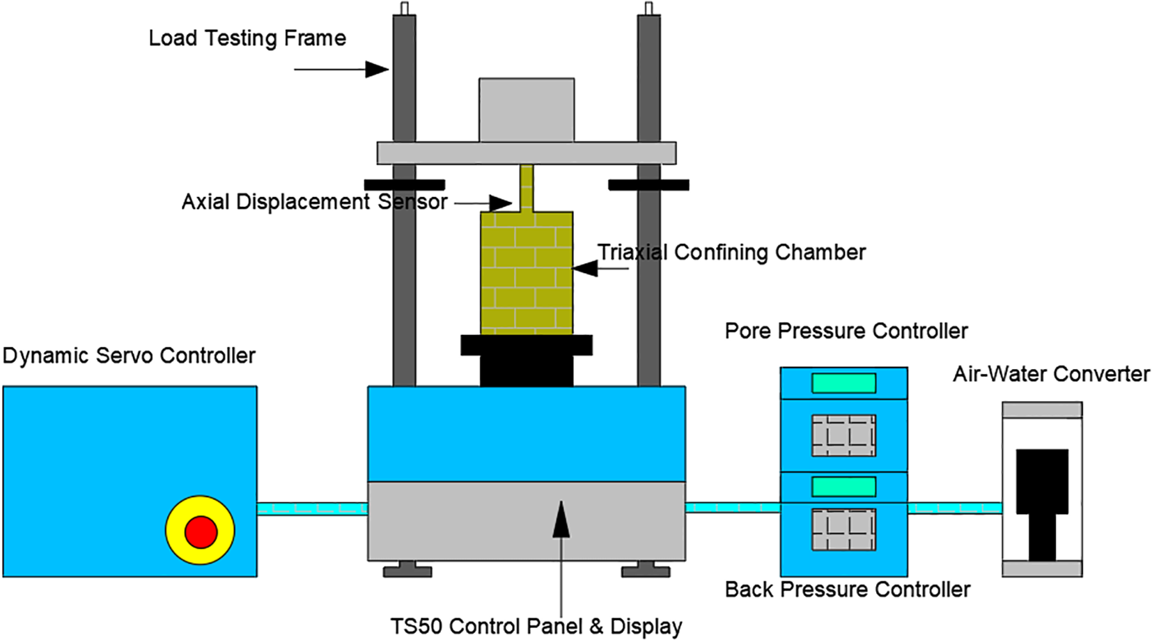
The instruments used in the study were static and dynamic triaxial testing systems from VJ Tech, UK. The apparatus primarily comprises a load frame with an integrated high-speed servo controller, an automatic confining pressure regulator, and an automatic back pressure regulator. The accompanying system software facilitates parameter setting, test control, and data acquisition, while also ensuring excellent interactive performance throughout the process. The instrument diagram is shown in Figure 1.
Figure 1
Static and dynamic triaxial testing systems.
2.2 Materials
2.2.1 Marine coral sand and clay
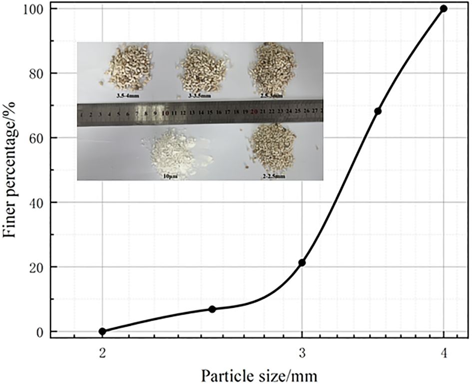
The materials employed in the test included marine coral sand and kaolin clay. The marine coral sand was sourced from an island in the South China Sea. After drying and screening, the 2-4 mm grain size fraction was selected for testing. The kaolin clay used had a grain size of 10 μm. Figure 2 shows the grain size distribution curve, and Table 1 enumerates the relevant parameters. The marine coral sand owned a non-uniformity coefficient of 1.32 and a curvature coefficient of 1.08, which indicated poor particle gradation.
Figure 2
Grain size grading curve of marine coral sand.
Table 1
| GS | D50/mm | Cc | Cu | emin | emax |
|---|---|---|---|---|---|
| 2.81 | 3.3 | 1.08 | 1.32 | 0.99 | 1.49 |
Basic physical parameters of marine coral sand.
2.2.2 3D printed polymer layer
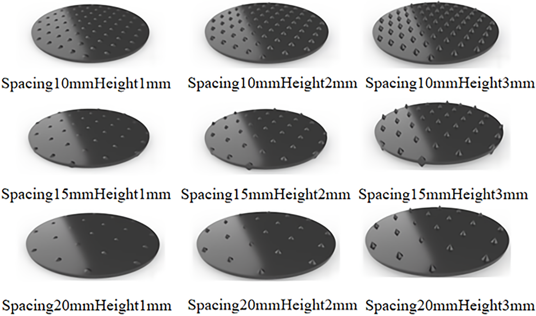
Polymer layer materials with various double-textured surfaces, which have surface asperity heights of 1 mm, 2 mm, and 3 mm, and spacings of 10 mm, 15 mm, and 20 mm, are fabricated through 3D printing technology (SLA). The textured surface of the polymer layer is conical, and the material used is white resin. Given the boundary effects during sample preparation and reinforcement, the polymer layer has a 96 mm diameter and a 2 mm thickness. Figure 3. shows the textured polymer layer model and the printed entity, while Table 2 provides detailed parameters of the polymer layer.
Figure 3
3D printing of polymer layer models.
Table 2
| Standard | Tensile modulus | Tensile strength | Elongation at break | Flexural modulus | Impact strength | Distortion temperature |
|---|---|---|---|---|---|---|
| ASTM | 2,450Mpa | 50Mpa | 10% | 2,400Mpa | 45J/m | 56°C |
Physical and mechanical properties of the polymer layer.
2.3 Testing program
The textured polymer layer’s potential reinforcement position is located in the shallow surface layer of the island in the South China Sea (Chao et al., 2024c), where the marine coral sand-clay mixture (MCCM) remains dry for extended periods and has very low water content due to prolonged sun exposure, which causes moisture evaporation (Chen et al., 2021). Yet, due to the inevitable wave action and the impact of extreme weather conditions such as heavy rainfall, seepage control must still be carefully considered. Therefore, the use of a polymer layer is essential to enhance stability and prevent potential damage in marine engineering applications. In this paper, however, MCCM is regarded as dry, which remains consistent with its condition in most ocean engineering applications. Unconsolidated undrained tests are performed to examine the mechanical properties of MCCM reinforced by textured polymer layers of varying surface types, confining pressures, and reinforcement layer numbers. These tests aim to minimize the effect of water content on the results. Given that marine coral sand particles are easy to break, particles are screened prior to and following the experiment to study the fragmentation characteristics of the MCCM under different conditions, and a quantitative analysis is performed. The sample dimensions are Φ100 mm × 200 mm, with a shear rate of 1 mm·min−¹. The details of the test design are provided in Table 3.
Table 3
| Number | Asperity spacing (mm) | Asperity height (mm) | Confining pressure (kPa) | Polymer layer layers |
|---|---|---|---|---|
| T1 | – | – | 10, 30, 50 | 0 |
| T2 | 10 | 1 | 10, 30, 50 | 1, 2 |
| T3 | 10 | 2 | 10, 30, 50 | 1, 2 |
| T4 | 10 | 3 | 10, 30, 50 | 1, 2 |
| T5 | 15 | 1 | 10, 30, 50 | 1, 2 |
| T6 | 15 | 2 | 10, 30, 50 | 1, 2 |
| T7 | 15 | 3 | 10, 30, 50 | 1, 2 |
| T8 | 20 | 1 | 10, 30, 50 | 1, 2 |
| T9 | 20 | 2 | 10, 30, 50 | 1, 2 |
| T10 | 20 | 3 | 10, 30, 50 | 1, 2 |
Experimental scheme.
2.4 Testing step
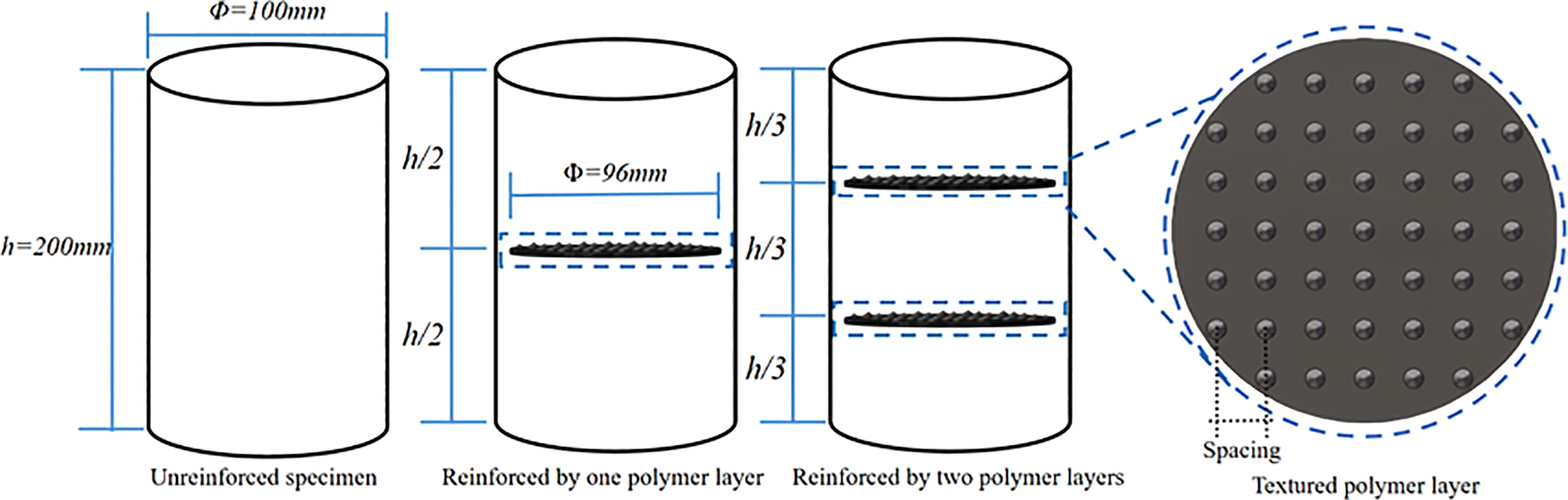
To minimize the impact of water content on experimental results, dry marine coral sand and kaolin clay are used for sample preparation, with a dry mass ratio of 58.8% marine coral sand to 41.2% kaolin clay (Xu et al., 2020; Zhao et al., 2025). Before sample preparation, marine coral sand and kaolin clay are blended in the specified proportions. The sample is prepared in six layers using a custom sand mold, with each layer compacted to a designated position. The reinforcement position diagram of the polymer layer is illustrated in Figure 4.
Figure 4
Polymer layer reinforcement position diagram.
After sample preparation, a triaxial compression test is conducted. The software automatically records axial force and strain data during the test and stops once the axial strain reaches 12%. Following the test, the MCCM undergoes cleaning, separation, drying, and screening. The gradation curve of marine coral sand particles after the test is obtained.
3 Methodology
3.1 Machine learning algorithms
In this study, a machine learning approach using a Back Propagation Neural Network (BPNN) is employed. To improve the model’s performance, various optimization techniques, such as Genetic Algorithm (GA), Particle Swarm Optimization (PSO), and Logical Development Algorithm (LDA), are integrated into the framework. These techniques provide several advantages, with three key benefits standing out in particular:
-
Each algorithm was developed using a consistent and systematic framework (Kardani et al., 2020).
-
These algorithms have been widely applied to address various challenges in the field of ocean engineering (Zhou et al., 2017).
-
They are highly effective in identifying complex nonlinear relationships between a variety of contributing variables (Liu et al., 2015).
3.1.1 BPNN
The Back Propagation Neural Network (BPNN) is an artificial neural network that processes data through multiple layers by iteratively adjusting weights and biases (Hecht-Nielsen, 1992). It takes input variables through the input layer, which are then propagated to the hidden layer, where weighted calculations and nonlinear transformations are performed using activation functions. The final output is the predicted result. In this study, the BPNN model is configured with five input parameters—Asperity spacing, Asperity height, confining pressure, number of reinforcement layers, and strain—and one output parameter: stress. The model uses the Log-Log Sigmoid function as the activation function and is built with the Newff function. Initial weights and biases are optimized to improve prediction accuracy. The BPNN model is shown in Figure 5.
Figure 5
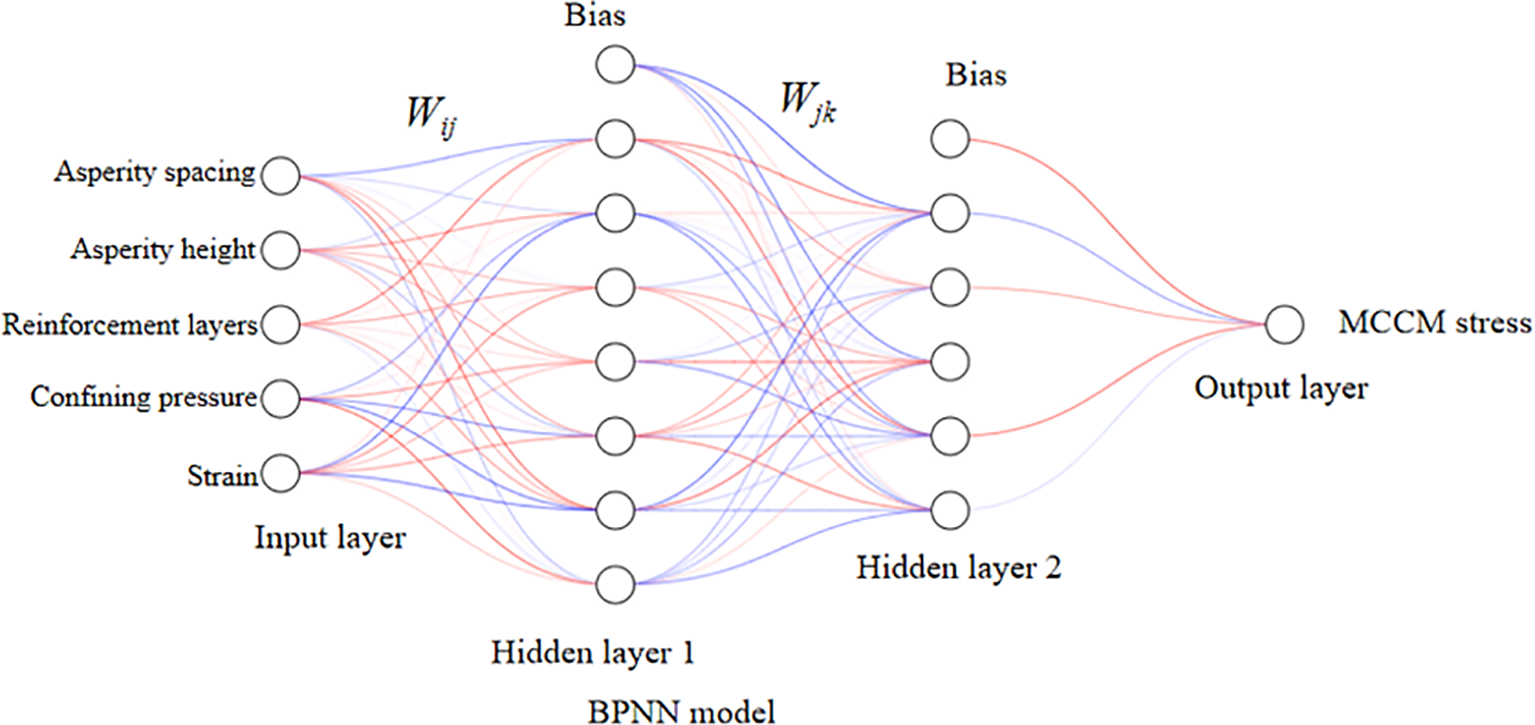
The typical structure of BPNN.
3.1.2 GA and PSO
The Genetic Algorithm (GA) is a population-based optimization method inspired by the principles of natural selection (Lambora et al., 2019). It seeks optimal or near-optimal solutions by simulating evolutionary processes like selection, crossover, and mutation. The process starts with a randomly initialized population, where each individual is evaluated using a fitness function. High-performing individuals are selected for reproduction, and genetic diversity is introduced through crossover and mutation. This iterative process continues until a stopping criterion, such as a maximum number of iterations or an acceptable fitness level, is met. GA is particularly effective in solving complex optimization problems due to its strong global search capability and adaptability in nonlinear, high-dimensional spaces.
Particle Swarm Optimization (PSO) is a population-based heuristic algorithm inspired by the coordinated behavior of swarming organisms, such as birds and fish (Wang et al., 2018). In PSO, each potential solution is represented as a particle that moves through the search space, adjusting its velocity and position based on both its personal best performance and the best result found by the entire swarm. This process allows the swarm to collectively converge on optimal solutions. PSO offers several advantages, including a simple structure, ease of implementation, no need for gradient information, and strong global optimization capabilities. It has been successfully applied in various optimization tasks, such as function optimization and neural network training.
3.1.3 LDA
The Logical Development Algorithm (LDA) is a supervised dimensionality reduction technique that reduces the dimensionality of input features by maximizing the ratio of between-class variance to within-class variance (Chao et al., 2024b). In regression tasks, LDA is used as a preprocessing step to extract the most relevant and uncorrelated features, which enhances model stability, reduces overfitting, and improves prediction accuracy. When integrated with neural networks, LDA simplifies the input space while preserving essential discriminative information, leading to more efficient and robust learning. The LDA-BPNN model is shown in Figure 6.
Figure 6
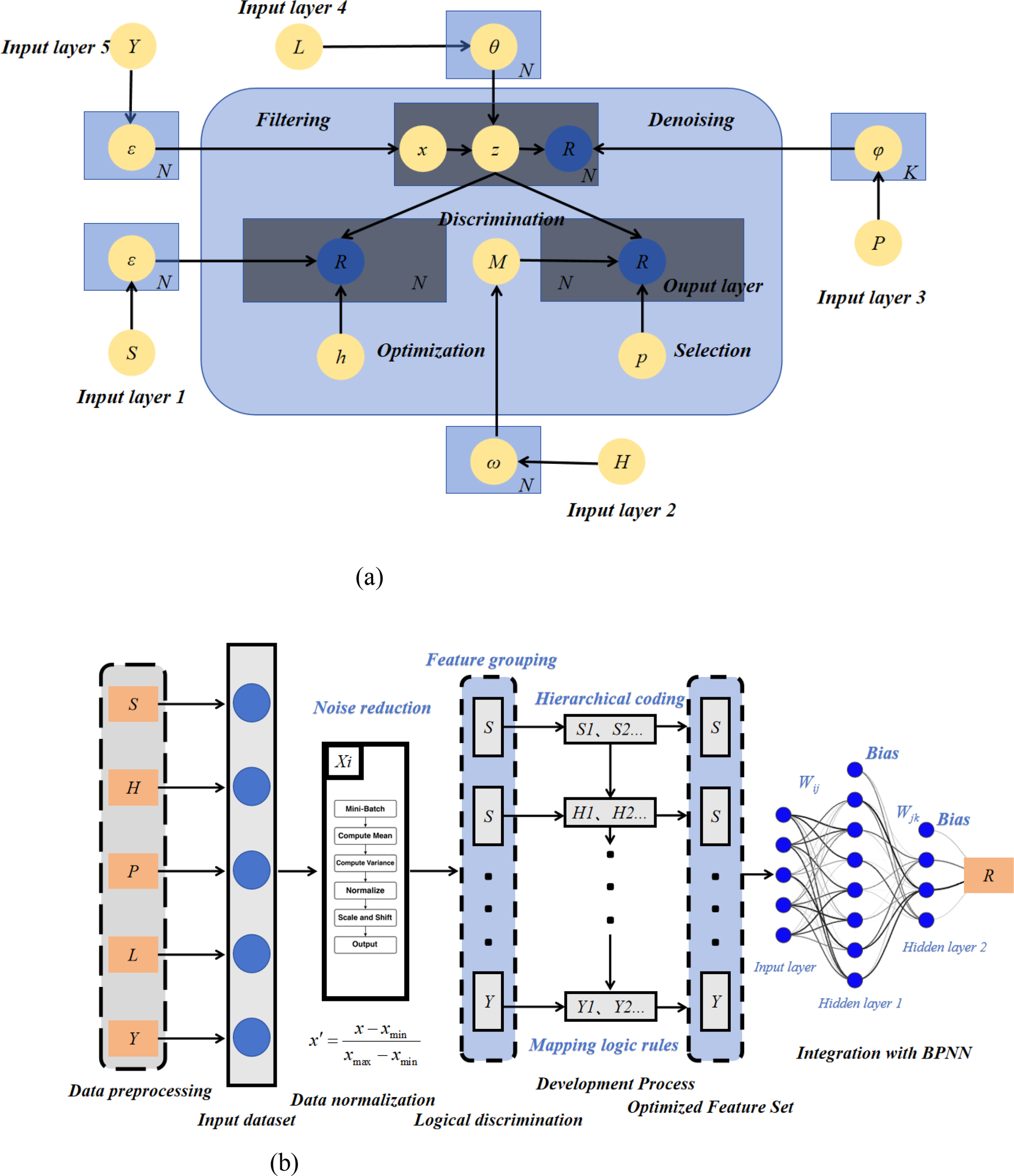
LDA-BPNN model workflow. (a) LDA structure diagram (b) The operation flow for LDA-BPNN.
3.2 Model parameter setting
3.2.1 Hyperparameter optimization
Optimizing hyperparameters is essential for improving the performance of machine learning models, as varying settings can greatly influence training efficiency and prediction accuracy. In this study, Genetic Algorithm (GA), Particle Swarm Optimization (PSO), and Logical Development Algorithm (LDA) were employed to enhance the hyperparameter tuning of a Backpropagation Neural Network (BPNN), thereby boosting its overall effectiveness.
To enhance convergence efficiency and prediction accuracy, key hyperparameters for each optimization algorithm were strategically configured, as detailed in Table 4. For the Genetic Algorithm (GA), the population size (pop_num) was set to 10 to balance computational cost with exploration capability. The number of generations (gen) was fixed at 80, allowing sufficient evolution without excessive runtime. The selection probability parameter (normGeomSelect) was adjusted to 0.1, increasing the likelihood of choosing high-fitness individuals. The crossover rate (arithXover) was defined as 2, promoting genetic diversity, while the mutation setting (nonUnifMutation) was specified as [0.3, 40, 2] to improve the algorithm’s global search behavior and prevent local optima entrapment. The convergence tolerance (maxGenTerm) was set at 1e-5, enabling continued refinement near optimal solutions. In the Particle Swarm Optimization (PSO) framework, cognitive and social learning factors (c1, c2) were each assigned a value of 2.0, ensuring a balanced influence between personal and group experiences on particle motion. The position search space was restricted to the interval [-2.0, 2.0], maintaining solution feasibility. A swarm size (sizepop) of 20 and a maximum iteration count (maxgen) of 120 were chosen to achieve a good compromise between search depth and computational load. The BPNN was trained with 200 epochs to provide adequate learning capacity. For the LDA approach, a population size of 25 and a maximum iteration count of 60 were selected. The mutation factor (F) was set at 0.6 to encourage robust global search, and the crossover probability (CR) was set at 0.85 to maintain population diversity during recombination. These settings allowed the model to better exploit class discriminative features during dimensionality reduction, thereby enhancing classification performance. Overall, the refined hyperparameter configurations for GA, PSO, and LDA significantly improved the BPNN’s performance by accelerating convergence, mitigating overfitting, and increasing predictive accuracy. These enhancements demonstrated strong applicability in tasks such as strength prediction of reinforced MCCM.
Table 4
| Hyperparameter | Parameter name | Range of values |
|---|---|---|
| GA | Population size(pop_num) | 10 |
| Genetic generations(gen) | 80 | |
| Selection function parameter(normGeomSelect) | 0.1 | |
| Crossover function parameter (arithXover) | 2 | |
| Mutation function parameter(nonUnifMutation) | [0.3,40,2] | |
| Optimal solution tolerance(maxGenTerm) | 1e-5 | |
| PSO | Learning factors (c1, c2) | 2 |
| Maximum position (popmax) | 2.0 | |
| Minimum position (popmin) | -2.0 | |
| Population size (sizepop) | 20 | |
| Population updates times (maxgen) | 120 | |
| Training iterations (epochs) | 200 | |
| LDA | Population size(pop_num) | 25 |
| Maximum number of iterations (max_iter) | 60 | |
| Mutation factor (F) | 0.6 | |
| Crossover probability (CR) | 0.85 |
Parameter settings for GA, PSO and LDA optimized BPNN.
Figure 7 presents a comparative analysis of RMSE trends for GA, PSO, and LDA throughout the optimization process. The horizontal axis denotes the number of iterations (0–50), while the vertical axis reflects RMSE values, representing the prediction error of the model. As observed, all three algorithms progressively reduce RMSE with increasing iterations, highlighting their capability to minimize prediction error effectively. Among them, PSO exhibits the fastest convergence, achieving lower RMSE values within fewer iterations, which indicates greater efficiency in navigating the solution space. However, after an initial sharp decline, PSO’s improvement rate slows and eventually plateaus at an RMSE of around 3. In comparison, GA also experiences a rapid early decrease in RMSE, followed by a steadier decline that levels off near 1.5 after roughly 20 iterations. LDA, meanwhile, begins with a slower reduction but accelerates in the later stages, ultimately converging to an RMSE close to 1. Overall, while PSO leads in early-stage convergence speed, LDA demonstrates superior final accuracy and stability, outperforming both GA and PSO in the long-term optimization performance.
Figure 7
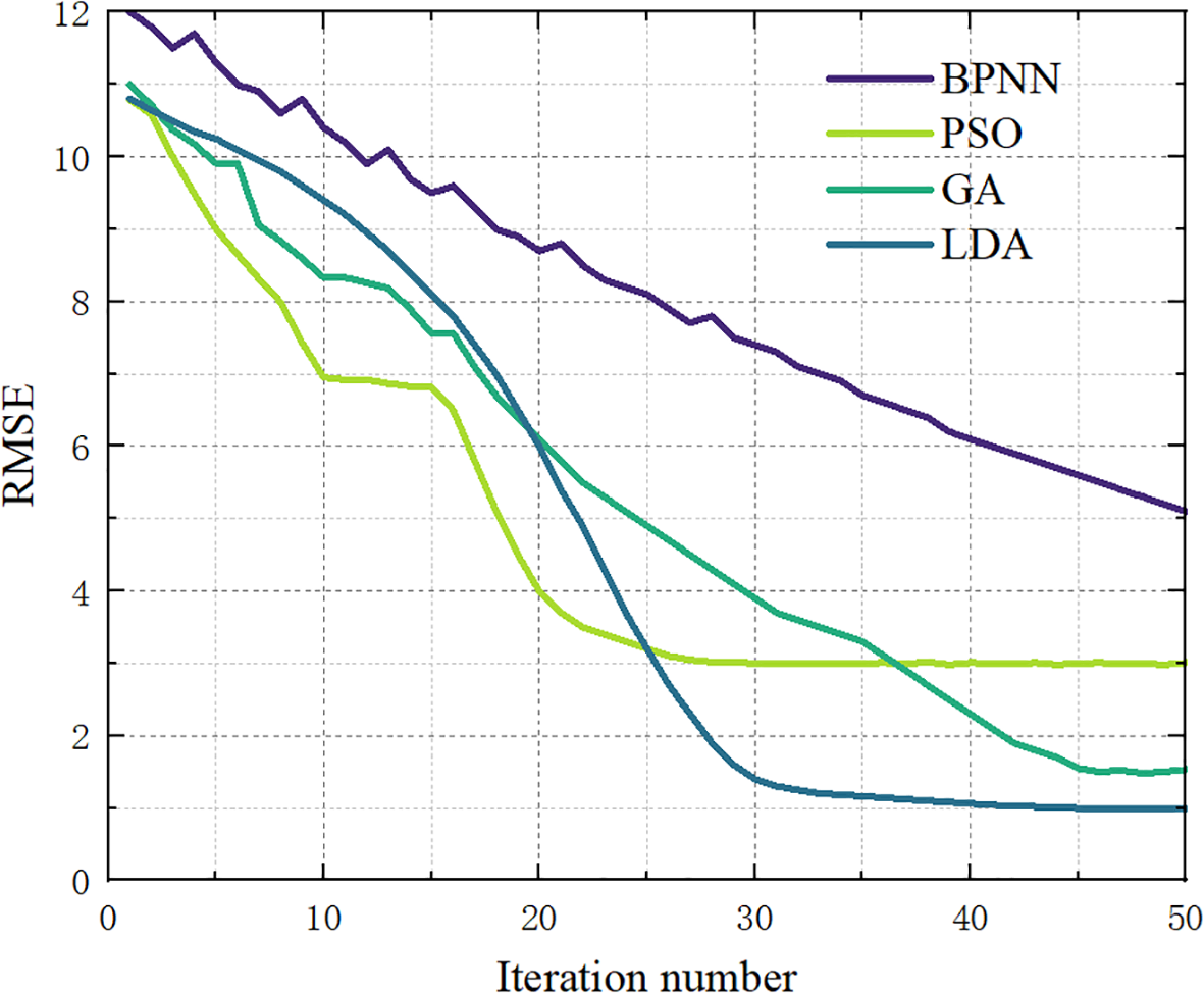
Number of RMSE iterations for GA, PSO and LDA.
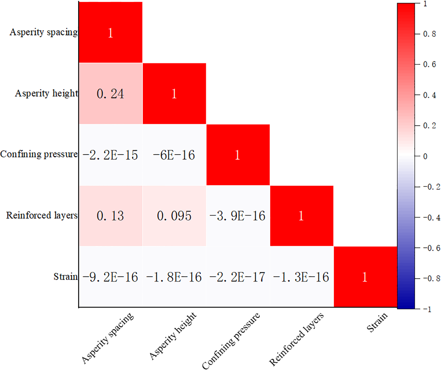
3.2.2 Establishment of database and data processing
To analyze the strength behavior of MCCM under varying conditions, a dataset of 2436 samples was developed. It includes five essential variables: asperity spacing, asperity height, confining pressure, number of reinforcement layers, and strain. To enhance the modeling efficiency and ensure consistency in data scale, all input and output variables were normalized prior to training. This normalization process helps accelerate model convergence and improves the overall predictive performance of the proposed machine learning model:
The summary statistics of the variables in the dataset are presented in Table 5. Asperity spacing ranges from 10 to 20 mm, while asperity height is categorized into three levels: 1 mm, 2 mm, and 3 mm. The number of reinforcement layers includes three levels: 0, 1, and 2. Confining pressure varies between 10 kPa and 50 kPa. The strain values span from 1% to 12%. To ensure data quality and the suitability for machine learning modeling, data preprocessing procedures were applied, including data cleaning, normalization, and dataset partitioning.
Table 5
| Argument | Type | Minimum value | Maximum value | Mean value | Standard deviation |
|---|---|---|---|---|---|
| Asperity spacing | Numerical type | 10 | 20 | 15 | 5 |
| Asperity height | 1 | 3 | 2 | 1 | |
| Confining pressure(Kpa) | 10 | 50 | 30 | 20 | |
| Number of reinforcement layers | 0 | 2 | 1 | 1 | |
| Strain(mm) | 1 | 12 | 7.27 | 3.26 |
Statistical table of factors affecting the stress of the MCCM.
3.2.3 Establishment of data sets
In this study, the dataset creation serves as the foundation for training the machine learning algorithms. A dataset with 5 input parameters and 1 output parameter was developed to train and validate the performance of BPNN, GA-BPNN, PSO-BPNN, and LDA-BPNN, as illustrated in Figure 8. The dataset was randomly divided into a training set (80%) and a testing set (20%) to ensure fair evaluation and minimize partitioning bias.
Figure 8
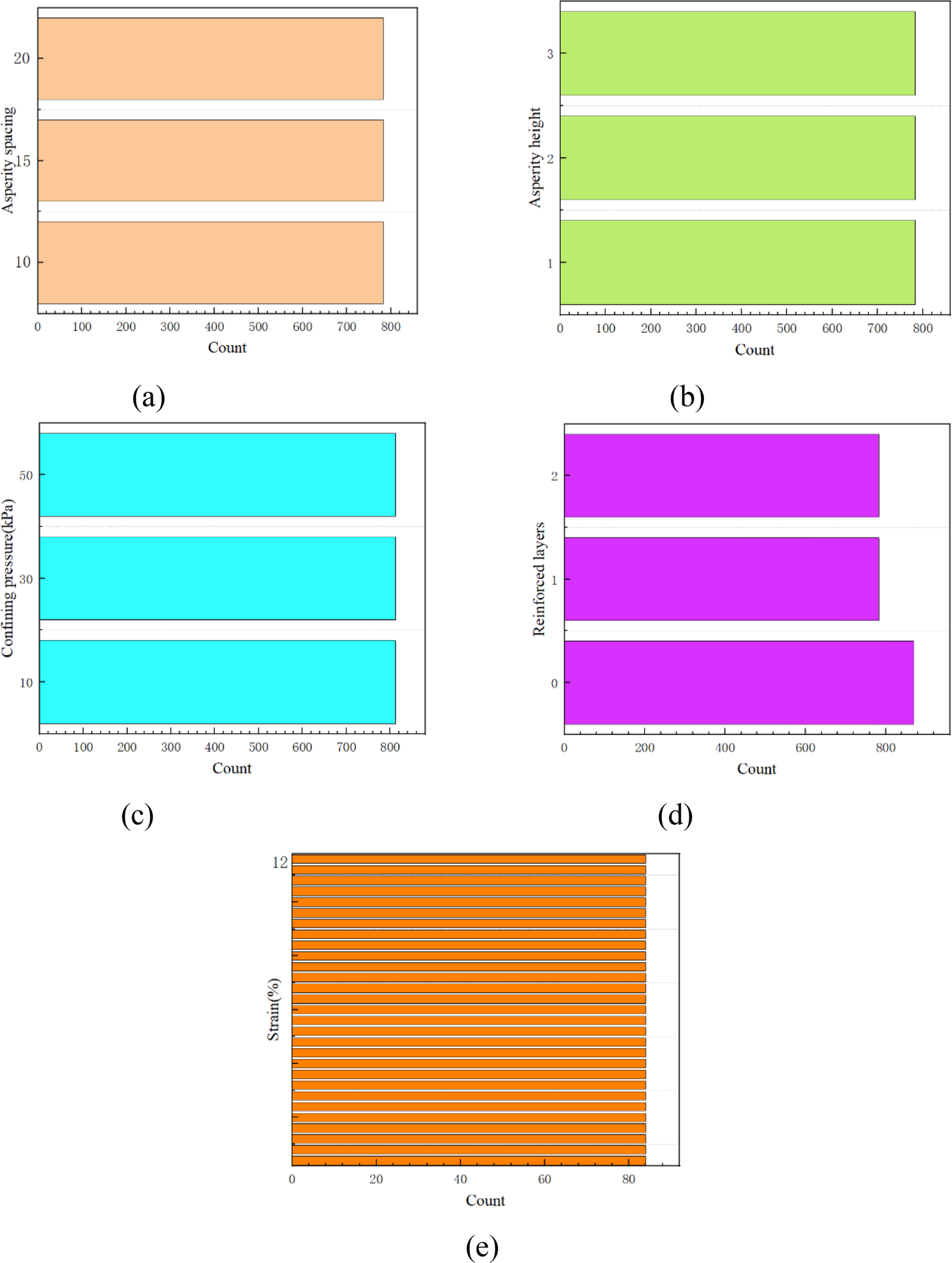
Distribution for data in the constructed database. (a) Asperity spacing (b) Asperity height (c) Confining pressure (d) Reinforced layers (e) Strain.
A total of 2,436 data samples were compiled, each comprising five critical input variables: asperity spacing, asperity height, confining pressure, number of reinforcement layers, and strain. To evaluate the model’s ability to generalize, the dataset was partitioned into two subsets: a training set and a testing set. The model was developed using the training data, while the test data was reserved for final performance validation. Specifically, 80% of the data was allocated for training and the remaining 20% for testing, enabling a reliable evaluation of the model’s predictive capability and real-world applicability. The parametric analysis diagram is shown in Figure 9.
Figure 9
Parametric analysis diagram.
3.3 Predictive performance assessment index
During model development and optimization, selecting suitable evaluation metrics is crucial for assessing predictive performance. In this study, two primary evaluation indicators are employed:
1, Root Mean Square Error (RMSE): This metric quantifies the standard deviation of the residuals between predicted and actual values. A lower RMSE signifies reduced prediction error, indicating higher model accuracy and reliability (Hodson, 2022). The RMSE calculation formula is shown in Equation 1.
Where n is the number of samples, yi is the observed value, and fi is the predicted value.
2, Mean Absolute Percentage Error (MAPE): This indicator measures the average absolute difference between predicted and actual values, expressed as a percentage of the actual values. A lower MAPE reflects smaller prediction deviations, indicating improved model accuracy and effectiveness (Chicco et al., 2021). The MAPE calculation formula is shown in Equation 2.
Where n is the number of samples, yi is the observed value, and is the predicted value.
4 Results and analysis of the experiment
4.1 Examination of sample failure patterns
After each test, the pressure chamber was disassembled, and the typical morphologies of the specimens with varying reinforcement layers after the test were recorded, as illustrated in Figure 10. Overall, the marine coral sand-clay mixture (MCCM) specimens did not show distinct shear planes and exhibited a bulging behaviour. In the unreinforced specimen, lateral bulging was most pronounced. With one layer of reinforcement, the bulging was reduced, primarily occurring above and below the reinforced area, where the textured polymer layer acted as a “belt” to restrain lateral bulging. With two layers of reinforcement, the bulging decreased further and became more evenly distributed across the top, middle, and bottom parts of the specimen, where the textured polymer layer acted like two ‘belts,’ further restricting the bulging. The phenomenon is similar to the one examined by some scholars (Ding et al., 2022). This phenomenon clearly shows that as the number of textured polymer layer reinforcement layers increases, the lateral bulging of the MCCM specimens is notably reduced.
Figure 10
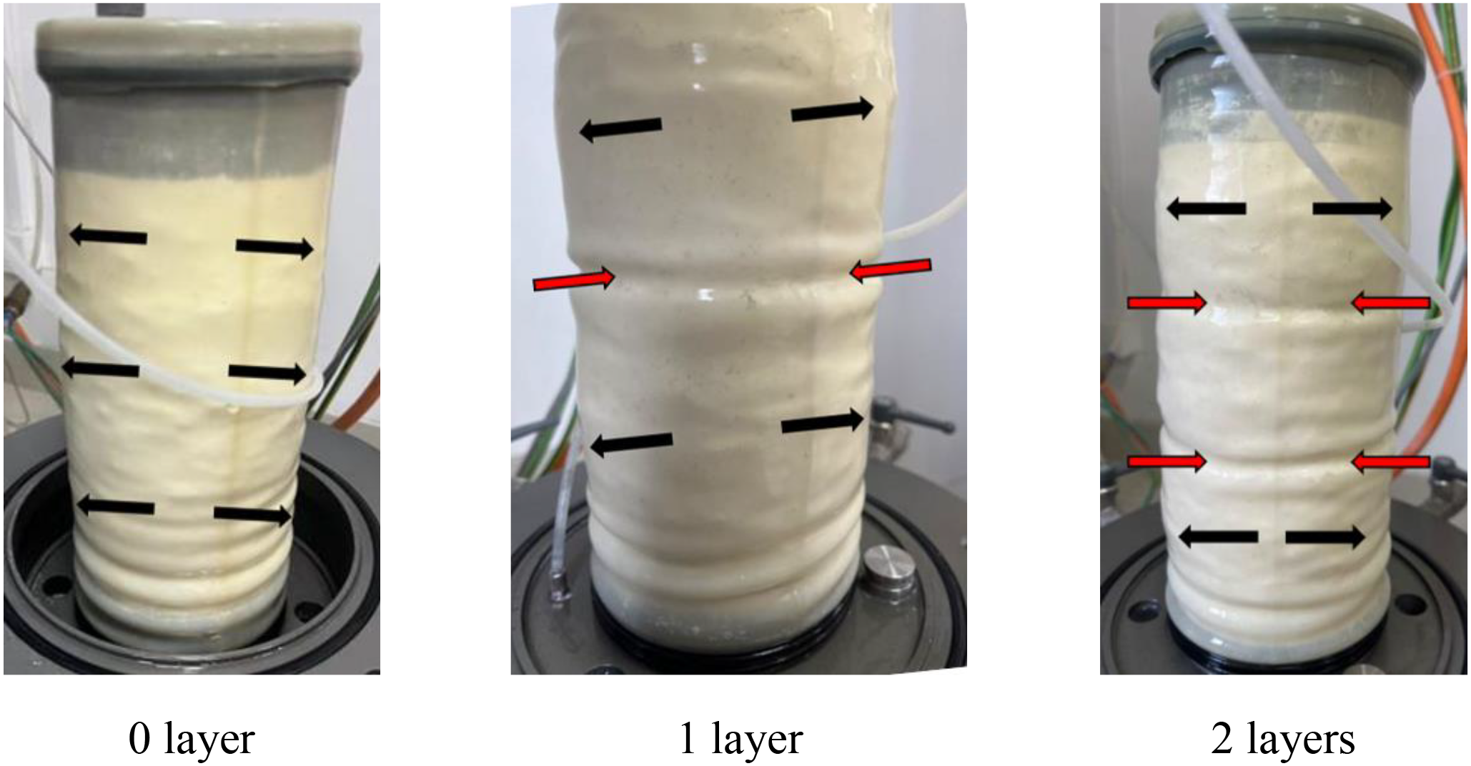
The failure modes of specimens with different numbers of reinforcement layers.
4.2 Deviatoric stress-strain relationship
Based on the experimental data, deviator stress-strain relationship curves were obtained for each experiment. Figure 11a presents the curves for plain MCCM under different confining pressures, which shows that the sample strength steadily rises with increased confining pressures. The deviator stress-strain curves exhibit a strain-hardening behaviour, which becomes more evident with increasing confining pressure. The maximum axial deviator stresses are 44.84 kPa, 110.44 kPa, and 214.70 kPa, respectively. Figures 11b–j present the deviator stress-strain curves for different types of textured polymer layers, various numbers of reinforcement layers, and confining pressures. As confining pressure and the number of reinforcement layers increase, the deviator stress-strain curves shift upward, the hardening trend becomes more evident, and shear strength steadily improves. When the confining pressure is 10 kPa, the deviator stress increases by up to 92.51%. At lower axial strains, the deviator stress-strain curves of reinforced and unreinforced MCCM samples almost overlap at the same confining pressure. With the increase in axial strain, the curves of the reinforced samples start to separate, clearly showing the reinforcement effect. With different types of textured polymer layers, the deviator stress-strain curves of the reinforced MCCM show only slight improvements, with minimal variations. The strength variations are not easily distinguishable from the deviator stress-strain curves. Section 4.3 analyses the impact of polymer layer surface texture size on MCCM strength by evaluating the strength enhancement rates of the reinforced samples.
Figure 11
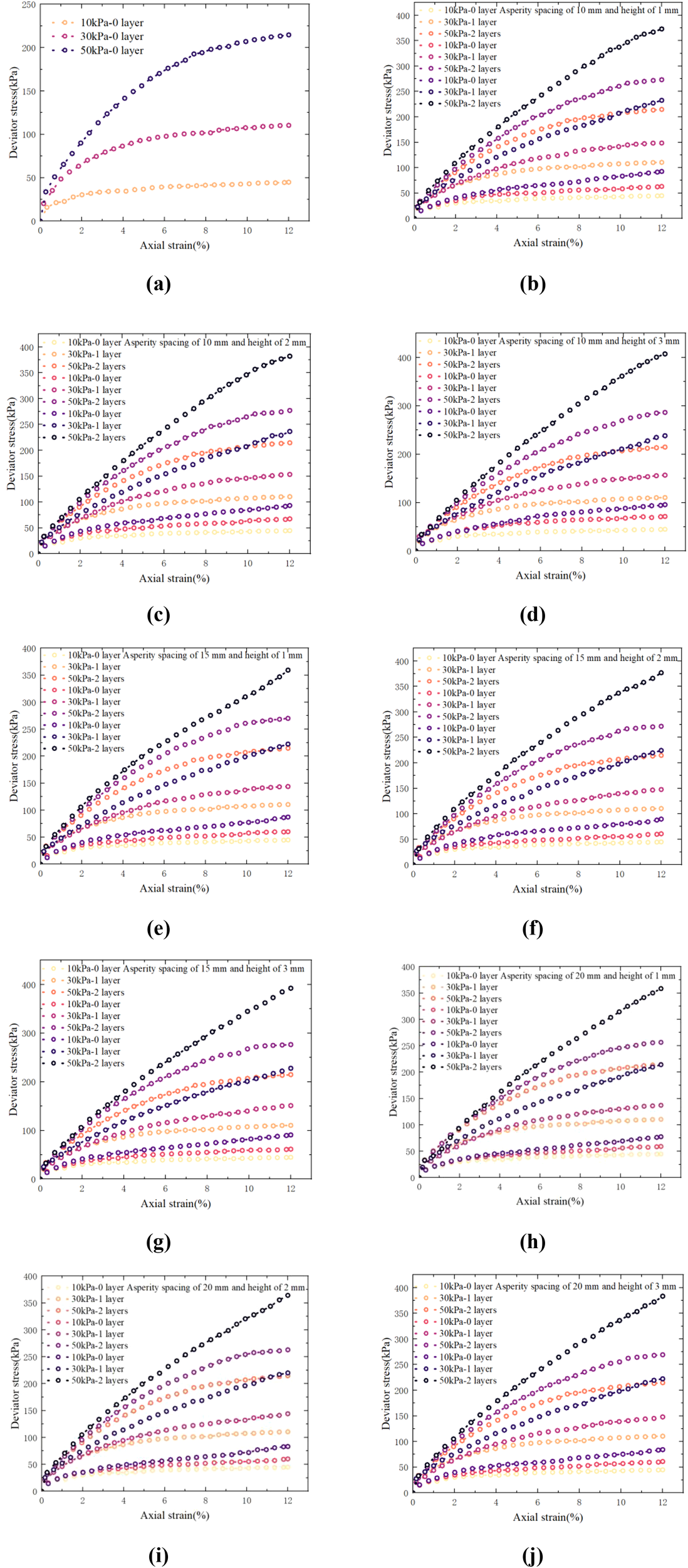
Deviator stress-strain curve: (a) T1; (b) T2; (c) T3; (d) T4; (e) T5; (f) T6; (g) T7; (h) T8; (i) T9; (j) T10.
4.3 Strength impact analysis
To better analyse the effects of different roughness types of polymer layers, confining pressure, and reinforcement layer numbers on the strength of MCCM, this study introduces the strength enhancement rate (Rs) and the Mohr-Coulomb failure criterion for quantitative analysis (Luo et al., 2024). According to the data shown in Figure 12, the strength enhancement rates under both reinforced and unreinforced conditions are observed. Figures 12a–c illustrate the strength enhancement rates under different types of polymer layers, confining pressures, and reinforcement layer numbers. The analysis indicates that polymer layer reinforcement can improve the strength of the MCCM to varying degrees. With an increase in reinforcement layers, the strength enhancement rate rises, while the strength enhancement rate generally decreases as the confining pressure increases. Under one and two reinforcement layers, the average strength enhancement rates increased by 26.92% and 74.39%, respectively. The three confining pressures (10kPa, 30kPa, 50kPa) showed average strength enhancement rates of 55.87%, 54.62%, and 41.47% under one and two reinforcement layers. Under different confining pressures and reinforcement layers, as the height of the asperity on the rough polymer layer surface increases and the spacing between them decreases, the strength enhancement rate slightly changes, with an overall increasing trend. In conclusion, under low confining pressures and multiple reinforcement layers, the reinforcement effect of rough polymer layers is optimal. The reinforcement effect is positively correlated with the increase in the height of asperity and the reduction in their spacing.
Figure 12
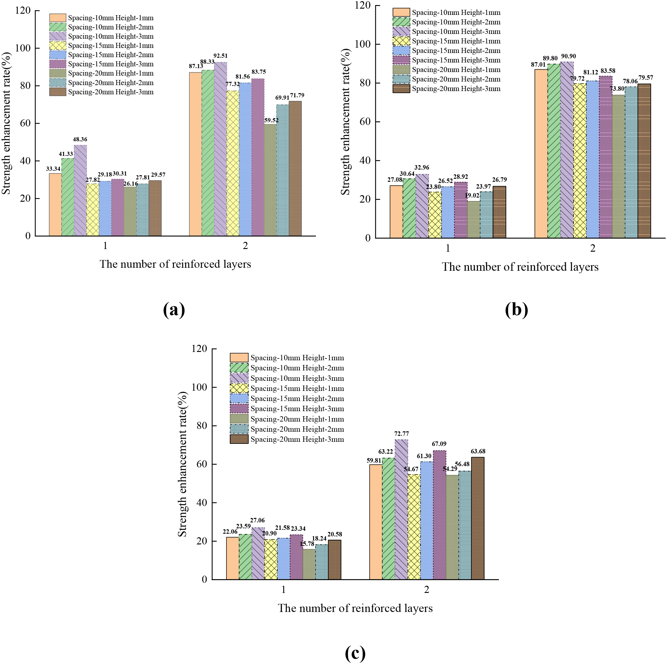
Strength enhancement ratio (a) 10kPa;(b) 30kPa;(c) 50kPa.
Additionally, the cohesion and internal friction angle of the MCCM specimens under various conditions were calculated, with results presented in Table 6 and Figure 13. From the table and image, it can be observed that the cohesion of MCCM under different conditions is very small, with similar values and no obvious pattern. Therefore, the average cohesion under different reinforcement layer numbers was calculated, showing a slight increase in cohesion with reinforcement. The internal friction angle of the MCCM specimens exhibits a more significant trend, increasing with the number of reinforcement layers. Under one and two reinforcement layers, the average internal friction angle increased by 6.77% and 15.58%, respectively, compared to the unreinforced samples. The larger the height of the asperity on the rough polymer layer surface, the larger the internal friction angle. However, the spacing between the asperity has little to no effect on the internal friction angle. It is evident that these nonlinear relationships are difficult to accurately describe using traditional methods, so this study will further explore these patterns using machine learning in section 4.5.
Table 6
| Number | 0 layer | 1 layer | 2 layers | |||
|---|---|---|---|---|---|---|
| c(kPa) | φ(°) | c(kPa) | φ(°) | c(kPa) | φ(°) | |
| T1 | 3.11 | 44.92 | – | – | – | – |
| T2 T3 |
– | – | 4.49 | 48.08 | 4.00 | 51.07 |
| – | – | 5.26 | 48.00 | 3.80 | 51.61 | |
| T4 | – | – | 6.05 | 48.62 | 4.35 | 53.47 |
| T5 | – | – | 4.09 | 48.21 | 3.54 | 50.67 |
| T6 | – | – | 3.88 | 48.07 | 4.05 | 52.01 |
| T7 | – | – | 3.69 | 48.30 | 4.07 | 53.00 |
| T8 | – | – | 4.57 | 47.25 | 1.71 | 51.36 |
| T9 | – | – | 4.05 | 47.39 | 2.68 | 51.35 |
| T10 | – | – | 3.90 | 47.74 | 2.86 | 52.76 |
| Average value | 3.11 | 44.92 | 4.44 | 47.96 | 3.45 | 51.92 |
Strength parameters of different test cases.
Figure 13
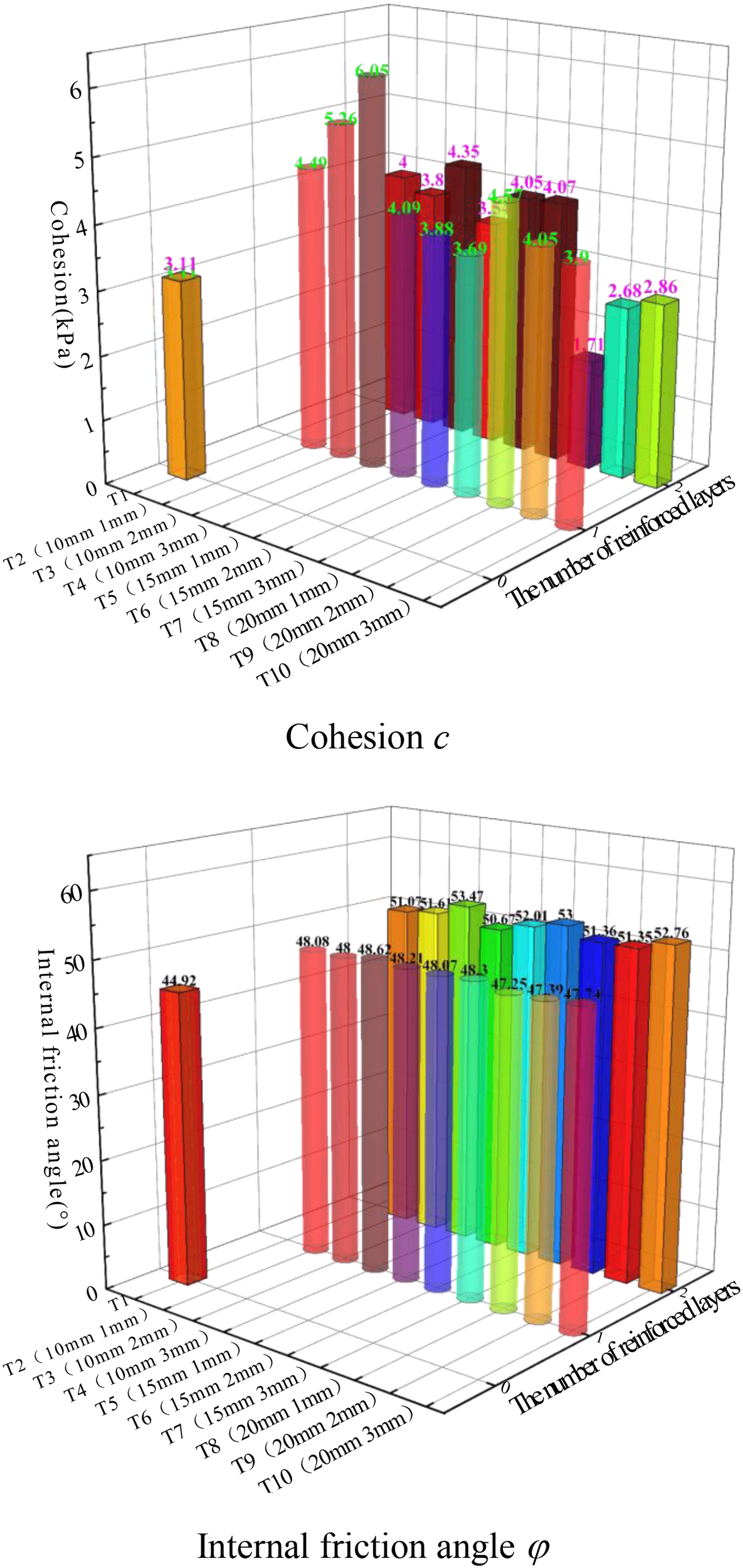
Cohesion c and internal friction angle φ.
4.4 Particle breakage analysis
The particle gradation data before and after the experiments (T1-T10) were obtained through sieving tests, and the corresponding curves were plotted. Figure 14 shows the particle gradation curves under different conditions. In Figure 14a, with an increase in confining pressure, the particle gradation curve gradually shifts upward, indicating an increase in the degree of particle breakage. Upon zooming in on the local curves, the particle breakage is concentrated between 2-2.5 mm. In Figures 14b–d, the degree of particle breakage increases with both the number of reinforcement layers and the confining pressure. However, due to the overlap of the particle gradation curves, the influence of different rough polymer layer types on particle breakage is not clearly discernible from the gradation curves. In all conditions, the particle breakage zone is concentrated between 2-2.5 mm.
Figure 14
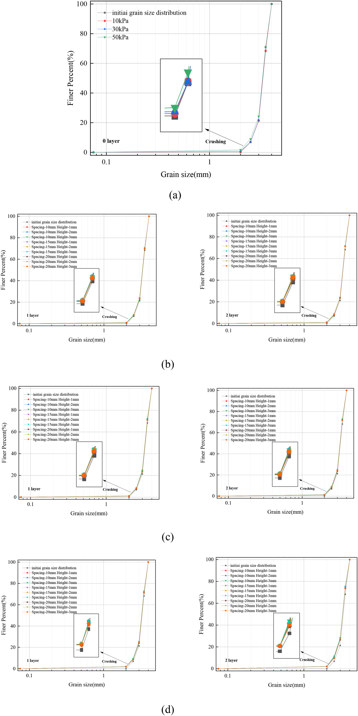
Particle grading curves before and after the experiment (a) 0layer;(b) 10kPa;(c) 30kPa;(d) 50kPa.
In conclusion, an increase in confining pressure and reinforcement layers leads to a greater degree of particle breakage, but the influence of different rough polymer layer types on particle breakage is not significant. Therefore, an attempt was made to analyse the particle breakage using the relative breakage rate (Br) (Hardin, 1985). The relative breakage rate Br diagram is shown in Figure 15. The Br values for all conditions (T1-T10) were calculated, as shown in Figure 16. The analysis indicates that the increase in reinforcement and confining pressure has a significant impact on particle breakage. As both confining pressure and the number of reinforcement layers increase, the relative breakage rate of MCCM significantly increases, with the maximum value of 3.84% occurring under two reinforcement layers and 50 kPa confining pressure. However, the effect of different polymer layer types on the particle breakage of marine coral sand is minimal. The general trend is that as the height of the asperities on the rough polymer layer surface increases and the spacing between them decreases, the particle breakage rate increases, but this effect is not pronounced.
Figure 15
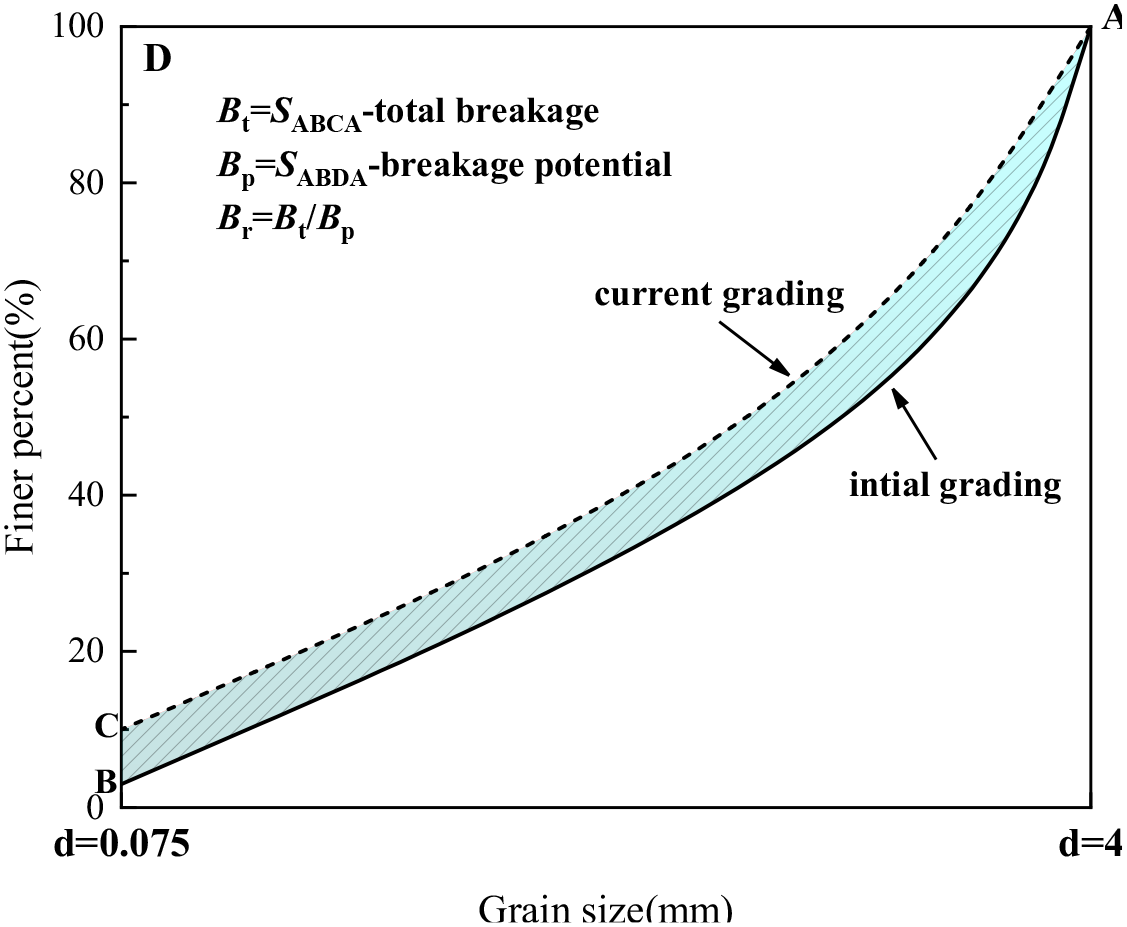
Relative breakage rate Br diagram.
Figure 16
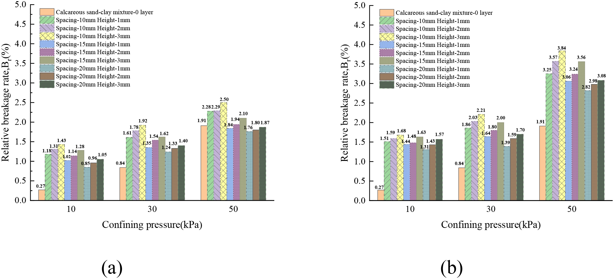
The relative breakage rates(Br) (a) 1 layer;(b) 2 layers.
In summary, particle breakage occurs in MCCM under all conditions, and the degree of particle breakage significantly increases with the increase in confining pressure and reinforcement layers. However, the change in the roughness of the rough polymer layer surface has a minimal effect on particle breakage. Therefore, particle breakage alone cannot accurately describe the pattern of MCCM strength variation. Its characteristics will be further detailed in the subsequent fractal dimension analysis and in Section 4.5 through machine learning.
To better quantify the state of particle breakage, the fractal model is used to characterize the particle breakage behaviour. Tyler and Wheatcraft (1992) introduced a fractal model for particle size distribution curves, representing the relationship between the cumulative mass of soil particles and particle size. The calculation formula is as follows:
Where d represents the size of the selected particle; M(d<di) represents the cumulative mass of particles with a diameter less than di; MT is the total mass of particles; di is the diameter of the ith layer of sieve, and the maximum particle size of marine coral sand is dmax; the slope α of the particle size distribution curve at the particle diameter di is given by α=3−D, where D is the fractal dimension of the particle material.
Taking the logarithm of both sides of (Equation 3) yields (Equation 4):
Based on equation (12), the slope k of the linear relationship between lg[M(d<di)/MT] and lg(di/dmax) is 3−D. Therefore, the fractal dimension D can be determined by calculating the slope of the curve on a log-log plot. A larger fractal dimension indicates a greater extent of particle fragmentation. The above equation is employed to describe the fractal behaviour of reinforced marine coral sand during triaxial compression tests. By examining the fractal dimension, we can conduct an in-depth study of the fractal breakage behaviour during the experimental process. Due to the relatively low confining pressure and other external loads, as well as the weakening effect of clay in this experiment, the breakage of marine coral sand particles was limited. Consequently, the particle size distribution curve does not reach the ultimate limit state of particle breakage. The final fractal dimension does not fall within the range specified by Equations 3 and 4. Therefore, the particle breakage characteristics of marine coral sand can only be quantitatively described by the specific variation patterns of the fractal dimension under different working conditions.
The particle sieving data from different experimental conditions were substituted into Equation 4, and the fractal dimension fitting curves, along with the fractal dimensions and fitting coefficients, were obtained through software, as shown in Figure 17 and Tables 7 and 8. Although the fractal behaviour is weak, the development of particle breakage can still be described by the gradually increasing fractal dimension. Upon analysis, it was found that the variation of the fractal dimension follows the same trend as the particle breakage rate. As the confining pressure and the number of reinforcement layers increase, the fractal dimension also increases. The effect of different rough polymer layer types on the fractal dimension is minimal. As the height of the asperities on the rough polymer layer surface increases and the spacing between them decreases, the fractal dimension also increases, but the increase is very small.
Figure 17
![Six scatter plots labeled (a) to (f), each showing the relationship between “lg(d/d_max)” on the x-axis and “lg[N(d<d)M^−1]” on the y-axis. Each plot features overlapping lines and markers with a legend indicating various object sizes and fitted curves, suggesting analysis of particle size distributions.](https://www.frontiersin.org/files/Articles/1653741/xml-images/fmars-12-1653741-g017.webp)
The fractal dimension curves under different conditions. (a) 10kPa 1layer (b) 10kPa 2layer (c) 30kPa 1layer (d) 30kPa 2layer (e) 50kPa 1layer (f) 50kPa 2layer.
Table 7
| Confining pressure (kPa) | D | R2 |
|---|---|---|
| 10 | -5.517 | 0.9601 |
| 30 | -4.513 | 0.9781 |
| 50 | -3.415 | 0.9853 |
The fractal dimension curves D&R2 under unreinforced conditions.
Table 8
| Confining pressure (kPa) | Asperity spacing (mm) | Asperity height (mm) | D | R 2 | ||
|---|---|---|---|---|---|---|
| 1 layer | 2 layer | 1 layer | 2 layer | |||
| 10 | 10 | 1 | -4.478 | -4.262 | 0.9722 | 0.9749 |
| 10 | 2 | -4.437 | -4.177 | 0.9720 | 0.9752 | |
| 10 | 3 | -4.347 | -4.058 | 0.9728 | 0.9763 | |
| 15 | 1 | -4.687 | -4.305 | 0.9697 | 0.9753 | |
| 15 | 2 | -4.582 | -4.261 | 0.9711 | 0.9756 | |
| 15 | 3 | -4.433 | -4.137 | 0.9719 | 0.9755 | |
| 20 | 1 | -4.994 | -4.442 | 0.9651 | 0.9747 | |
| 20 | 2 | -4.803 | -4.349 | 0.9675 | 0.9743 | |
| 20 | 3 | -4.630 | -4.264 | 0.9702 | 0.9738 | |
| 30 | 10 | 1 | -4.270 | -4.155 | 0.9742 | 0.9738 |
| 10 | 2 | -4.119 | -3.931 | 0.9746 | 0.9767 | |
| 10 | 3 | -4.082 | -3.839 | 0.9760 | 0.9779 | |
| 15 | 1 | -4.345 | -4.274 | 0.9753 | 0.9748 | |
| 15 | 2 | -4.263 | -4.071 | 0.9741 | 0.9765 | |
| 15 | 3 | -4.180 | -4.005 | 0.9748 | 0.9759 | |
| 20 | 1 | -4.184 | -4.351 | 0.9730 | 0.9759 | |
| 20 | 2 | -4.341 | -4.181 | 0.9745 | 0.9766 | |
| 20 | 3 | -4.208 | -4.144 | 0.9764 | 0.9754 | |
| 50 | 10 | 1 | -3.306 | -3.164 | 0.9851 | 0.9808 |
| 10 | 2 | -3.284 | -3.136 | 0.9856 | 0.9794 | |
| 10 | 3 | -3.225 | -3.084 | 0.9855 | 0.9785 | |
| 15 | 1 | -3.340 | -3.174 | 0.9873 | 0.9817 | |
| 15 | 2 | -3.291 | -3.183 | 0.9871 | 0.9804 | |
| 15 | 3 | -3.179 | -3.158 | 0.9878 | 0.9794 | |
| 20 | 1 | -3.391 | -3.226 | 0.9873 | 0.9845 | |
| 20 | 2 | -3.341 | -3.205 | 0.9875 | 0.9836 | |
| 20 | 3 | -3.326 | -3.186 | 0.9879 | 0.9831 | |
The fractal dimension curves D&R2 under reinforced conditions.
4.5 Machine learning predicting performance
The predictive performance of the machine learning model, trained and evaluated on 2,436 samples, is illustrated in Figures 18 and 19. All training sets are shown in Figures 18a, c, e, g; all test sets are shown in Figures 18b, d, f, h.
Figure 18
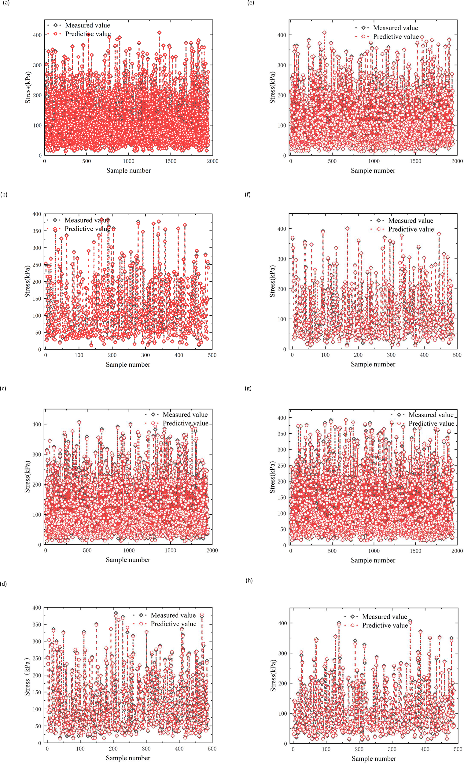
Prediction results of training set and test set on test data. (a) BPNN training dataset (b) BPNN test dataset (c) GA training dataset (d) GA test dataset (e) PSO training dataset (f) PSO test dataset (g) LDA training dataset (h) LDA test dataset.
Figure 19
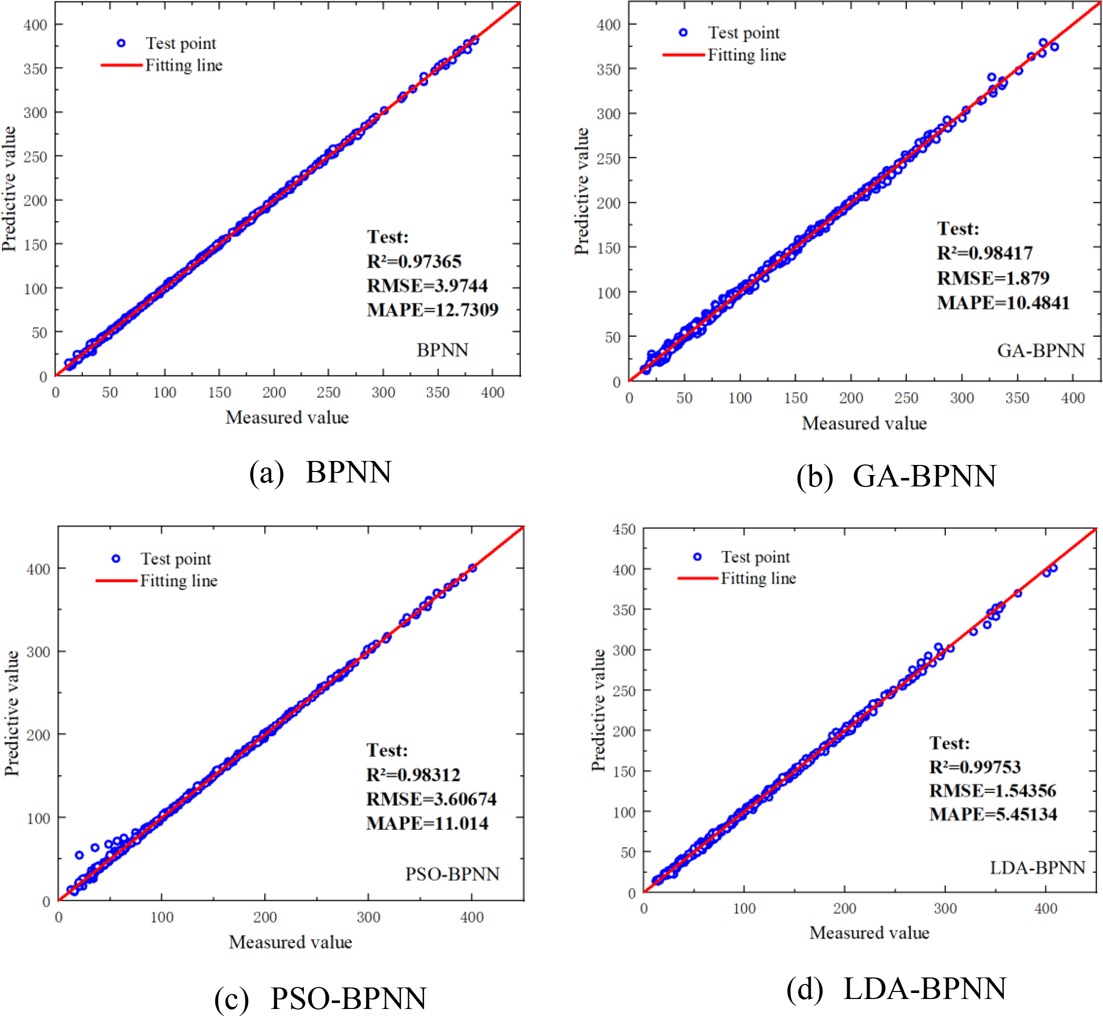
Fitting lines of different models.
Overall, the predicted outputs (represented by red hollow circles) generated by each model exhibit a generally good agreement with the actual values (black hollow diamonds), suggesting that all models are capable of capturing the underlying nonlinear relationships between the input features and the target variable to a certain extent. This alignment indicates their effectiveness in fitting the training data. However, noticeable discrepancies in prediction accuracy exist among the models, highlighting differences in their learning capabilities. Among the models evaluated, the LDA-BPNN model (Figure 18h) demonstrates the highest predictive accuracy, with its outputs showing minimal deviation from the observed values. This suggests that the LDA-BPNN model not only achieves precise fitting but also maintains a strong capacity to model complex interactions in the data. In contrast, the standard BPNN model (Figure 18b) exhibits larger prediction errors, especially in samples with high peak values. These deviations imply that the shallow architecture of the BPNN lacks the representational power required to fully capture intricate data patterns, leading to underfitting in more complex regions of the dataset. Improvements are observed in the GA-BPNN (Figure 18d) and PSO-BPNN (Figure 18f) models, both of which integrate optimization techniques—Genetic Algorithm and Particle Swarm Optimization, respectively—to enhance the baseline BPNN. These hybrid models yield predictions that more closely follow the actual trends, indicating better parameter tuning and improved model robustness. Nonetheless, signs of mild overfitting are apparent in certain samples, particularly in regions with relatively high data variance, which suggests the need for further regularization or cross-validation to enhance generalization.
In summary, the LDA-BPNN model consistently outperforms the other approaches across both training and testing datasets. Its strong fitting accuracy, combined with stable generalization to unseen data, underscores its effectiveness in modeling the complex relationships present in the input space, making it the most robust and reliable choice among the models evaluated in this study.
As illustrated in Figure 19, the LDA-BPNN model consistently outperforms the other three machine learning models when evaluated on the testing dataset. Specifically, LDA-BPNN model achieves the highest prediction accuracy, recording the lowest RMSE values of 1.54356 for the testing set and 1.23474 for the training set. Additionally, it yields the minimum MAPE values—5.45134% for the testing set and 7.22231% for the training set—demonstrating strong generalization capability. The model also achieves the highest correlation coefficient (R) of 0.99753 on the test data, indicating a very strong linear relationship between the predicted and actual values.
In comparison, although the GA-BPNN model benefits from genetic algorithm optimization and shows improved performance over the base model, it still lags behind LDA-BPNN. The GA-BPNN model reports RMSE values of 1.5397 and 1.879 for the test and training sets, respectively, and MAPE values of 5.9479% and 10.4841%. Its test set R value of 0.98417 suggests a moderately strong correlation, but the model exhibits limitations in fully capturing the underlying data patterns.
The PSO-BPNN model performs relatively poorly, with larger prediction errors and more dispersed residuals. This indicates that the integration of particle swarm optimization does not significantly enhance the predictive power of the base BPNN. For this model, the RMSE values for the test and training sets are 3.60674 and 3.85794, respectively, while the corresponding MAPE values are 9.451% and 11.014%. The test set correlation coefficient (R) is 0.98312, reflecting reduced predictive consistency.
The original BPNN model exhibits the weakest performance among all four models. It produces the highest RMSE values of 3.81524 and 3.9744, and MAPE values of 9.2679% and 12.7309% for the test and training datasets, respectively. With an R value of 0.97365, coupled with a noticeable deviation between predicted points and the regression line, the results suggest that the shallow architecture of BPNN lacks the capacity to effectively represent the complex, nonlinear interactions in the dataset.
In summary, the LDA-BPNN model demonstrates superior performance in both training and testing phases compared to GA-BPNN, PSO-BPNN, and BPNN. It offers higher predictive accuracy, stronger generalization, and more robust model stability—especially on unseen data. Even under similar optimization strategies, the LDA-BPNN approach delivers significantly better predictive capabilities than the other models.
4.6 Sensitivity analysis
Understanding the internal mechanisms of machine learning models is essential for enhancing model transparency, interpretability, and practical trustworthiness. A key component of this understanding lies in analyzing feature importance, which helps to reveal how different input variables influence the model’s predictions and provides valuable insights into the decision-making process (Yang et al., 2025). Among the various interpretability techniques available, the Shapley Additive Explanations (SHAP) method has emerged as one of the most effective and widely adopted tools. Rooted in cooperative game theory, SHAP systematically considers all possible combinations of input features to evaluate how each one contributes to a given prediction. For each individual prediction, SHAP assigns a numerical value—referred to as the SHAP value—to every input feature. This value quantifies the marginal contribution of that feature to the model’s output. A positive SHAP value indicates that the feature increases the predicted output, while a negative value suggests a reducing effect (Lundberg and Lee, 2017). By aggregating SHAP values across multiple samples, researchers and practitioners can identify which features have the most influence on the model across the entire dataset, as well as understand local variations in individual predictions. This level of interpretability is particularly valuable for complex models such as neural networks or ensemble methods, where traditional coefficient-based explanations fall short. SHAP thus not only supports technical validation and model refinement, but also helps promote the responsible and informed deployment of machine learning in real-world applications.
Figure 20 presents the five most influential features affecting the output of the LDA-BPNN model and provides a quantitative assessment of their individual contributions. The pie chart illustrates the mean SHAP values for each feature, where a higher SHAP value indicates a greater contribution to the model’s prediction. On the left, the swarm plot offers a more detailed visualization of feature effects: the x-axis represents SHAP values, indicating the direction and magnitude of each feature’s impact on the prediction, while the y-axis corresponds to the feature values. A high SHAP value combined with a high feature value typically suggests a positive correlation—larger feature values lead to increased predicted outputs. Conversely, negative SHAP values imply a suppressive influence on the model’s output within certain value ranges. Among all the features, Asperity spacing emerges as the most dominant factor, contributing 32.7% to the overall prediction. This highlights its critical role in governing the stress-strain behavior of MCCM, likely due to its influence on shear resistance at the contact interface—wider spacing enhances interfacial friction, thereby improving the composite strength. Asperity height ranks second in importance, with a contribution of 27.5%. Its impact is attributed to enhanced mechanical interlocking; greater asperity heights intensify particle interlock, promoting energy dissipation and increasing shear resistance during deformation.
Figure 20
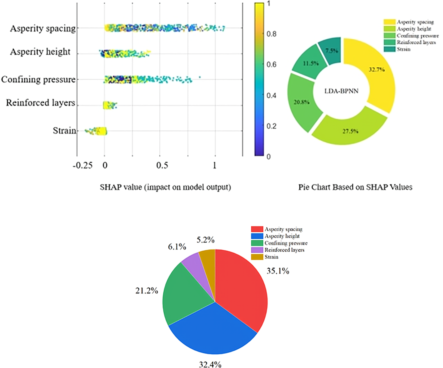
Feature importance analysis plot. (a) All of the sample (b) A single sample.
In contrast, strain itself shows the lowest average SHAP value at only 7.5%, suggesting it has limited direct influence on the model output. This may indicate that strain is more a response variable dependent on other input features rather than a primary predictor. The SHAP-based interpretability analysis clearly identifies Asperity spacing as the leading determinant in the model’s predictive performance. This finding underscores the importance of carefully controlling and optimizing asperity spacing in the engineering design of MCCM-based materials. Likewise, the substantial influence of Asperity height signifies its role in enhancing interfacial mechanical behavior.
In summary, the results reveal considerable variation in the contributions of different features to the prediction accuracy. Therefore, targeted optimization strategies should prioritize high-impact parameters—particularly asperity spacing and height—to ensure the structural stability, safety, and durability of marine infrastructure constructed with MCCM under complex environmental conditions.
4.7 Empirical formulas
Previous modeling results demonstrate that the developed LDA-BPNN model is capable of accurately predicting the strength of MCCM. Nevertheless, the inherent complexity of machine learning models can pose practical challenges, particularly for engineers and practitioners lacking expertise in artificial intelligence. To enhance usability and facilitate broader application, this section introduces an analytical empirical expression that replicates the predictive behavior of the LDA-BPNN model. This formulation provides a straightforward and efficient means for estimating MCCM strength. The BPNN employed follows a standard feedforward architecture with a single hidden layer. Its output can be represented by a mathematical expression derived from the trained connection weights and node biases, as shown below (Goh et al., 2005):
The normalized predicted output Yn, ranging from -1 to 1, is calculated based on the normalized input variables Xi, which includes asperity spacing (mm),asperity height(mm), number of reinforcement layers, confining pressure (kPa), and strain (%), through the connection weights Wik between the ith input node and the kth hidden node, hidden layer biases bk, weights Wk connecting the hidden nodes to the output node, output layer bias b0, and the hyperbolic tangent sigmoid transfer function , where h and m denote the numbers of hidden nodes and input variables, respectively.
The normalized output Yn can be converted into the actual predicted strength τ using the following denormalization formula (Equation 6):
Here, τmax and τmin represent the maximum and minimum MCCM strength values in the dataset, respectively.
To facilitate engineering applications, the neural network structure described above can be further expressed in the following simplified form. As shown in Equations 7–9.
All connection weights in the model (Wik, Wk) and bias parameters (bk, b0) are automatically optimized during training using the Differential Evolution algorithm. The complete set of parameters, which can be directly applied in ocean engineering calculations, is provided in Table 9.
Table 9
| Hidden layer node number | Weight | Bias | ||||||
|---|---|---|---|---|---|---|---|---|
| Input parameter | Output parameter | Hidden layer | Output layer | |||||
| S | H | P | L | Y | R | |||
| 1 | 0.42 | -0.44 | 0.21 | 0.44 | -0.27 | 0.23 | 1.05 | 0.51 |
| 2 | 1.18 | 1.16 | -0.14 | 1.03 | 0.15 | -0.18 | -0.72 | |
| 3 | 0.91 | -1.32 | 1.05 | -1.15 | 0.57 | 0.12 | 0.45 | |
| 4 | -1.12 | 0.34 | -1.17 | 1.78 | -0.93 | 0.03 | 0.84 | |
| 5 | 1.24 | 1.45 | 0.92 | -1.67 | 1.23 | -0.01 | 1.09 | |
Connected weights and biases for the constructed LDA-BPNN algorithm.
This analytical empirical model offers strong interpretability and enables rapid prediction of MCCM strength without relying on machine learning platforms, making it well-suited for practical engineering scenarios where model transparency and computational efficiency are critical.
The input variables S, H, P, L, and Y correspond to asperity spacing, asperity height, confining pressure, number of reinforced layers, and strain, respectively. The output variable R represents the strength of the MCCM, as detailed in Table 9.
4.8 Experimental verifications
To assess the applicability and accuracy of the machine learning model and the analytical formula, the proposed empirical model was used to predict the strength of MCCM under various conditions. A total of 30 representative test cases were selected, as detailed in Table 10. Based on the specific experimental setups, Equation 5 was employed to estimate the strength of MCCM under different scenarios. The predicted results were then compared with experimental data from previous studies, as illustrated in Figure 21. This comparison served to evaluate the predictive performance and practical value of the developed model across a range of conditions.
Table 10
| Asperity spacing | Asperity height | Confining pressure (kPa) | Reinforced layers | Strain (%) |
|---|---|---|---|---|
| 0 | 0 | 10 | 0 | 5 |
| 30 | 0 | 8 | ||
| 50 | 0 | 12 | ||
| 10 | 1 | 10 | 1 | 1 |
| 2 | 30 | 2 | 3 | |
| 3 | 50 | 1 | 5 | |
| 10 | 1 | 50 | 2 | 7 |
| 2 | 10 | 1 | 9 | |
| 3 | 30 | 2 | 12 | |
| 10 | 1 | 30 | 1 | 10 |
| 2 | 50 | 2 | 8 | |
| 3 | 10 | 1 | 4 | |
| 15 | 1 | 10 | 1 | 1 |
| 2 | 30 | 2 | 3 | |
| 3 | 50 | 1 | 5 | |
| 15 | 1 | 50 | 2 | 7 |
| 2 | 10 | 1 | 9 | |
| 3 | 30 | 2 | 12 | |
| 15 | 1 | 30 | 1 | 10 |
| 2 | 50 | 2 | 8 | |
| 3 | 10 | 1 | 4 | |
| 20 | 1 | 10 | 1 | 1 |
| 2 | 30 | 2 | 3 | |
| 3 | 50 | 1 | 5 | |
| 20 | 1 | 50 | 2 | 7 |
| 2 | 10 | 1 | 9 | |
| 3 | 30 | 2 | 12 | |
| 20 | 1 | 30 | 1 | 10 |
| 2 | 50 | 2 | 8 | |
| 3 | 10 | 1 | 4 |
30 sets of data selected for the experiment.
Figure 21
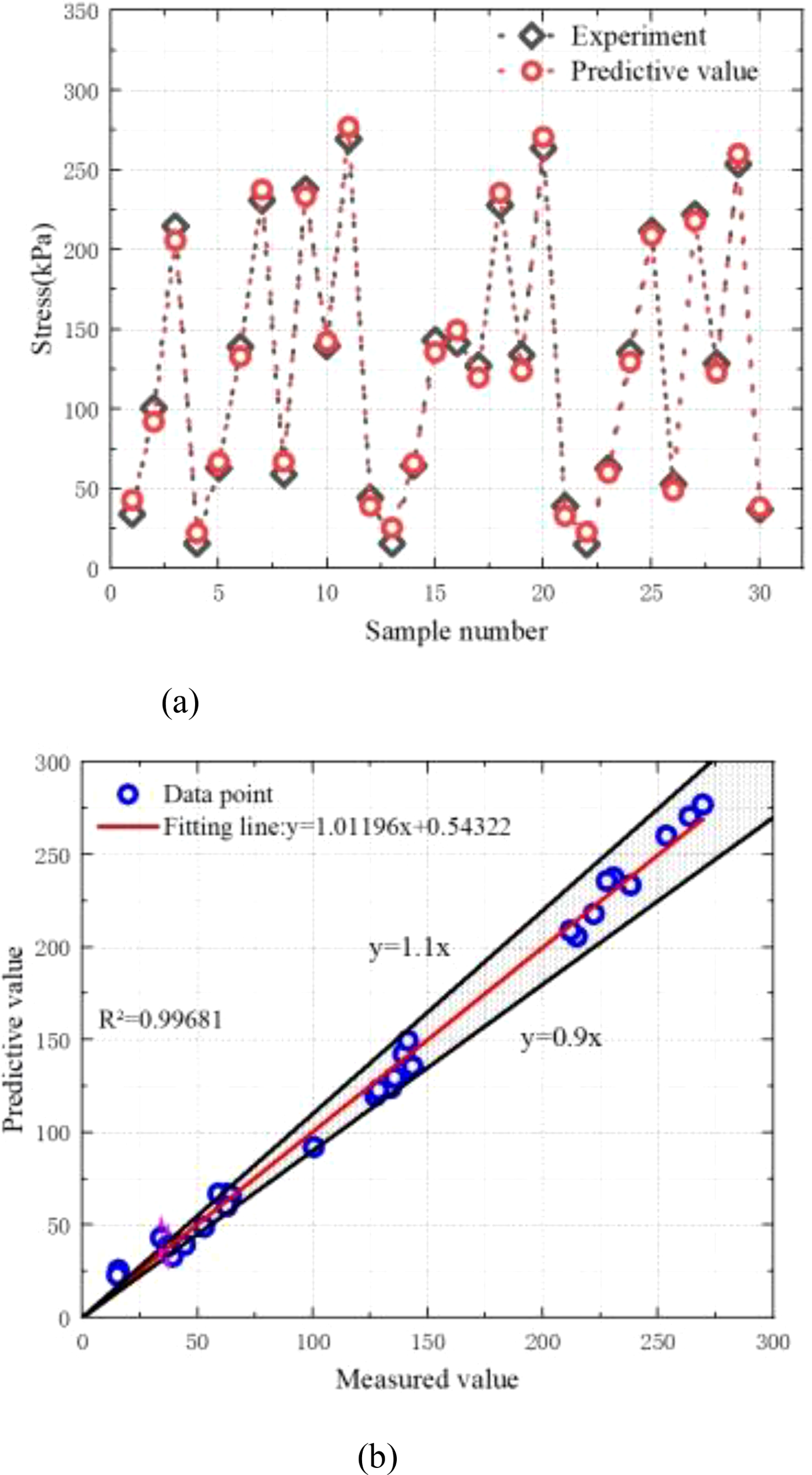
Performance evaluation of MCCM strength prediction based on empirical equations (a) The predicted value and experiment data (b) The R2 value.
As illustrated in Figures 21, the developed empirical prediction formula demonstrates excellent performance in estimating the strength of marine coral sand–clay mixtures (MCCM) under various conditions. The model yields a root mean square error (RMSE) of 1.112, a mean absolute percentage error (MAPE) of 5.65%, and a coefficient of determination (R²) of 0.99681, indicating exceptional predictive accuracy and robustness. These results confirm the model’s capability in effectively capturing the strength behavior of MCCM across different scenarios.
Compared with more complex machine learning-based approaches, the proposed formula offers enhanced practicality and accessibility, particularly for engineering professionals without backgrounds in programming or algorithm development. Its transparent structure and interpretable parameters make it a straightforward and efficient alternative for rapid strength estimation. This approach not only reduces technical barriers in modeling and analysis but also serves as a reliable tool for engineering design, construction planning, and safety evaluation. Overall, it holds significant promise for broader application and dissemination in marine engineering practice.
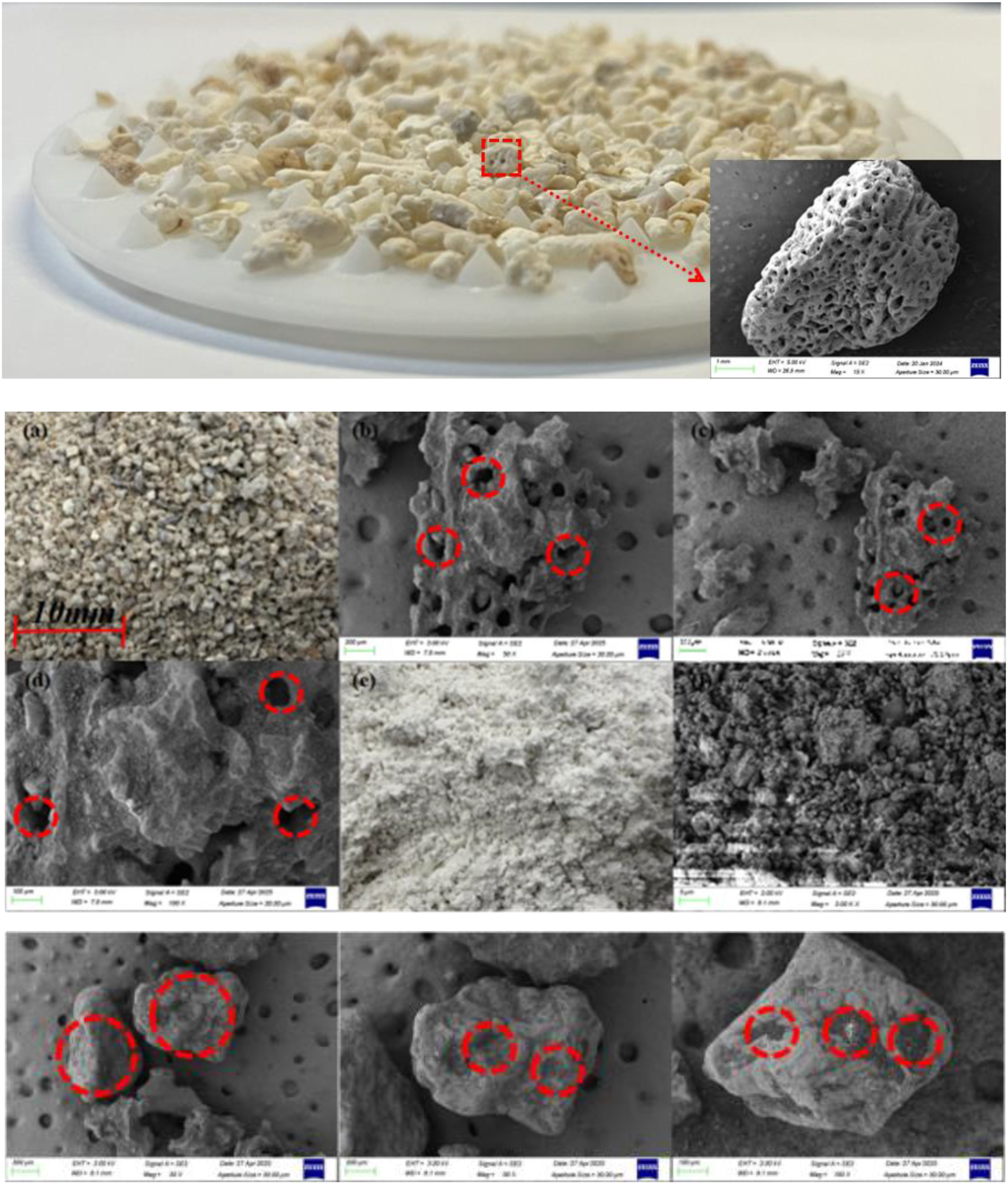
5 Discussion of the interface properties
Figure 22 presents scanning electron microscope (SEM) images that reveal the complex interface interaction mechanism between the marine coral sand-clay mixture (MCCM) and the polymer layer reinforcement. MCCM consists of angular marine coral sand particles with high porosity and flaky clay minerals. This unique composition creates a more complex and mechanically robust interlocking interface with the polymer layer. The rough polymer layer primarily acts as a constraint through its asperities, which limit the lateral movement of the marine coral sand. Additionally, the polymer layer, with its membrane-like, non-perforated structure, also restricts the longitudinal movement of the sand.
Figure 22
The interface diagram and SEM image.
As shown in Figure 22, fine clay particles infiltrate the voids between the marine coral sand particles, forming a denser skeletal structure. This “filling and coating” effect not only reduces the overall porosity of the mixture but also significantly increases the effective bonding area between the MCCM and the polymer layer. Especially on the surface of the polymer layer, clay particles exhibit strong adhesion, further enhancing the interface contact. In summary, the microscopic interaction mechanisms at the interface between the polymer layer and MCCM include:
-
Clay filling and coating the pores of the marine coral sand;
-
Adhesion between the clay and the polymer layer surface;
-
Mechanical interlocking between the angular sand particles and the asperity structure.
These synergistic effects collectively enhance the interface strength and overall stability of the reinforced MCCM system, providing a solid microstructural foundation for its application in the reinforcement of marine soft soils and island and reef engineering.
6 Conclusion
This study investigates the mechanical behaviour of marine coral sand-clay mixtures (MCCM) reinforced with 3D-printed textured polymer layers through a series of laboratory tests, including unconsolidated undrained triaxial compression tests, particle size distribution analysis, and SEM observations. The effects of asperity height (1-3 mm), spacing (10-30 mm), number of reinforcement layers (1-2), and confining pressure (10-50 kPa) on stress-strain response, strength, and particle breakage were systematically evaluated. Based on the test results, a comprehensive database was established, and an LDA-BPNN model was developed to predict the strength of MCCM using key variables such as asperity spacing, asperity height, confining pressure, reinforcement layers, and strain. To assess model performance, three benchmark models (BPNN, GA-BPNN, PSO-BPNN) were developed for comparison. A sensitivity analysis was conducted to quantify the influence of each input variable, and an empirical formula was derived to support engineering applications without requiring machine learning expertise. The main findings are summarized as follows:
-
As reinforcement layers and confining pressure increase, MCCM strength improves, with deviatoric stress-strain curves shifting upward and hardening more pronounced. Reinforced samples show a 15%–92% strength increase over unreinforced ones, with maximum gains of 48.36% for single-layer and 92.51% for double-layer reinforcement. The reinforcing effect is minimal at low axial strains but becomes more significant as strain increases.
-
The strength enhancement rate increases with the number of reinforcement layers, asperity height, and reduced asperity spacing. The highest rate, 92.51%, occurs at 10 kPa confining pressure with two reinforcement layers. Reinforced samples show higher cohesion (up to 4.44 kPa) and internal friction angles (up to 51.92°) than unreinforced ones.
-
Particle breakage in MCCM under triaxial compression is minor, mainly occurring in the 2–2.5 mm range. Confining pressure and reinforcement layers significantly influence breakage, peaking at 3.84% under 50 kPa with two layers.
-
The study identifies asperity spacing, asperity height, confining pressure, reinforcement layers, and strain as the primary factors influencing MCCM strength, with asperity spacing and height showing the most significant strengthening effects. The LDA-BPNN model demonstrated superior predictive accuracy and generalization. Sensitivity analysis confirmed asperity spacing as the most influential parameter. Furthermore, the derived empirical formula offers clear interpretability and practical utility, enabling reliable strength predictions without the need for advanced machine learning tools—an efficient solution for data-limited engineering applications.
-
The interface characteristics of textured polymer layer-reinforced MCCM are mainly governed by frictional constraints within the asperities. SEM reveals diverse marine coral sand shapes with porous, textured surfaces, increasing friction and enhancing interaction with the polymer layer.
Statements
Data availability statement
The original contributions presented in the study are included in the article/Supplementary Material. Further inquiries can be directed to the corresponding author.
Author contributions
DS: Conceptualization, Formal Analysis, Funding acquisition, Investigation, Methodology, Project administration, Resources, Supervision, Validation, Visualization, Writing – review & editing. KX: Conceptualization, Data curation, Formal Analysis, Methodology, Project administration, Software, Validation, Visualization, Writing – original draft. XY: Conceptualization, Formal Analysis, Methodology, Software, Supervision, Validation, Writing – original draft. ZC: Conceptualization, Data curation, Formal Analysis, Methodology, Resources, Validation, Visualization, Writing – review & editing. PC: Conceptualization, Formal Analysis, Funding acquisition, Methodology, Project administration, Resources, Software, Supervision, Validation, Visualization, Writing – review & editing.
Funding
The author(s) declare financial support was received for the research and/or publication of this article. The authors would like to acknowledge the consistent support of National Natural Science Foundation of China: No 52471290, No 52301327; Project funded by China Postdoctoral Science Foundation: No 2024T170217, No 2023M730929; Failure Mechanics and Engineering Disaster Prevention, Key Lab of Sichuan Province: No FMEDP202209; Shanghai Sailing Program: No 22YF1415800, No 23YF1416100; Shanghai Natural Science Foundation: No 23ZR1426200, No 24ZR1427900; The Shanghai Soft Science Key Project: No 23692119700; Funded by Key Laboratory of Ministry of Education for Coastal Disaster and Protection, Hohai University, No 202302; Funded by Key Laboratory of Estuarine & Coastal Engineering, Ministry of Transport, No KLECE202302.
Conflict of interest
The authors declare that the research was conducted in the absence of any commercial or financial relationships that could be construed as a potential conflict of interest.
Generative AI statement
The author(s) declare that no Generative AI was used in the creation of this manuscript.
Publisher’s note
All claims expressed in this article are solely those of the authors and do not necessarily represent those of their affiliated organizations, or those of the publisher, the editors and the reviewers. Any product that may be evaluated in this article, or claim that may be made by its manufacturer, is not guaranteed or endorsed by the publisher.
References
1
Bacas B. M. Konietzky H. Berini J. C. Sagaseta C. (2011). A new constitutive model for textured geomembrane/geotextile interfaces. Geotext. Geomembr.29, 137–148. doi: 10.1016/j.geotexmem.2010.10.014
2
Chao Z. Fowmes G. (2021). Modified stress and temperature-controlled direct shear apparatus on soil-geosynthetics interfaces. Geotext. Geomembr.49, 825–841. doi: 10.1016/j.geotexmem.2020.12.011
3
Chao Z. Fowmes G. (2022). The short-term and creep mechanical behaviour of clayey soil-geocomposite drainage layer interfaces subjected to environmental loadings. Geotext. Geomembr.50, 238–248. doi: 10.1016/j.geotexmem.2021.10.004
4
Chao Z. Li Z. Dong Y. Shi D. Zheng J. (2024a). Estimating compressive strength of coral sand aggregate concrete in marine environment by combining physical experiments and machine learning-based techniques. Ocean Eng.308, 118320. doi: 10.1016/j.oceaneng.2024.118320
5
Chao Z. Liu H. Wang H. Dong Y. Shi D. Zheng J. (2024b). The interface mechanical properties between polymer layer and marine sand with different particle sizes under the effect of temperature: Laboratory tests and artificial intelligence modelling. Ocean Eng.312, 119255. doi: 10.1016/j.oceaneng.2024.119255
6
Chao Z. Ma G. He K. Wang M. (2021). Investigating low-permeability sandstone based on physical experiments and predictive modeling. Undergr. Space6, 364–378. doi: 10.1016/j.undsp.2020.05.002
7
Chao Z. Shi D. Fowmes G. Xu X. Yue W. Cui P. et al . (2023). Artificial intelligence algorithms for predicting peak shear strength of clayey soil-geomembrane interfaces and experimental validation. Geotext. Geomembr.51, 179–198. doi: 10.1016/j.geotexmem.2022.10.007
8
Chao Z. Shi D. Zheng J. (2024c). Experimental research on temperature–Dependent dynamic interface interaction between marine coral sand and polymer layer. Ocean Eng.297, 117100. doi: 10.1016/j.oceaneng.2024.117100
9
Chao Z. Wang H. Hu S. Wang M. Xu S. Zhang W. (2024d). Permeability and porosity of light-weight concrete with plastic waste aggregate: Experimental study and machine learning modelling. Construct. Building Mater.411, 134465. doi: 10.1016/j.conbuildmat.2023.134465
10
Chao Z. Wang M. Sun Y. Xu X. Yue W. Yang C. et al . (2022). Predicting stress-dependent gas permeability of cement mortar with different relative moisture contents based on hybrid ensemble artificial intelligence algorithms. Construct. Building Mater.348, 128660. doi: 10.1016/j.conbuildmat.2022.128660
11
Chao Z. Wang H. Zheng J. Shi D. Li C. Ding G. et al . (2024e). Temperature-dependent post-cyclic mechanical characteristics of interfaces between geogrid and marine reef sand: experimental research and machine learning modeling. J. Mar. Sci. Eng.12, 1262. doi: 10.3390/jmse12081262
12
Chen X. Dai G. Liu H. Ouyang H. Gong W. (2024). A microstructural investigation on hydraulic conductivity of calcareous clay. Appl. Ocean Res.150, 104133. doi: 10.1016/j.apor.2024.104133
13
Chen Q. Yu R. Tao G. Zhang J. Nimbalkar S. (2021). Shear behavior of polyurethane foam adhesive improved calcareous sand under large-scale triaxial test. Mar. Georesour. Geotechnol.39, 1449–1458. doi: 10.1080/1064119X.2020.1849473
14
Cheng L. Hossain M. Hu Y. Kim Y. Ullah S. N. (2022). A simple breakage model for calcareous sand and its FE implementation. J. Geotech. Geoenviron. Eng.148, 04022065. doi: 10.1061/(ASCE)GT.1943-5606.0002834
15
Chicco D. Warrens M. J. Jurman G. (2021). The coefficient of determination R-squared is more informative than SMAPE, MAE, MAPE, MSE and RMSE in regression analysis evaluation. Peerj Comput. Sci.7, e623. doi: 10.7717/peerj-cs.623
16
Ding X.-M. Luo Z.-G. Ou Q. (2022). Mechanical property and deformation behavior of geogrid reinforced calcareous sand. Geotext. Geomembr.50, 618–631. doi: 10.1016/j.geotexmem.2022.03.002
17
Giroud J. Han J. Tutumluer E. Dobie M. (2023). The use of geosynthetics in roads. Geosynth. Int.30, 47–80. doi: 10.1680/jgein.21.00046
18
Goh A. T. Kulhawy F. H. Chua C. (2005). Bayesian neural network analysis of undrained side resistance of drilled shafts. J. Geotech. Geoenviron. Eng.131, 84–93. doi: 10.1061/(ASCE)1090-0241(2005)131:1(84)
19
Han S. Jung S. Na W.-B. (2020). Estimation of seabed settlement during initial installation of a box-type artificial reef considering different seabed soil compositions and incident angles. Ocean Eng.218, 108269. doi: 10.1016/j.oceaneng.2020.108269
20
Hardin B. O. (1985). Crushing of soil particles. J. Geotech. Eng.111, 1177–1192. doi: 10.1061/(ASCE)0733-9410(1985)111:10(1177)
21
Hecht-Nielsen R. (1992). Theory of the backpropagation neural network, Neural networks for perception. Elsevier, 65–93. doi: 10.1016/B978-0-12-741252-8.50010-8
22
Hodson T. O. (2022). Root mean square error (RMSE) or mean absolute error (MAE): When to use them or not. Geosci. Model. Dev. Discuss.2022, 1–10. doi: 10.5194/gmd-15-5481-2022
23
Jie J. Zeng J. Ren Y. (2004). Improved mind evolutionary computation for optimizations, Fifth World Congress on Intelligent Control and Automation (IEEE Cat. No. 04EX788). IEEE, 2200–2204. doi: 10.1109/WCICA.2004.1341978
24
Jin H. Guo L. Sun H. Shi L. Cai Y. (2022). Undrained cyclic shear strength and stiffness degradation of overconsolidated soft marine clay in simple shear tests. Ocean Eng.262, 112270. doi: 10.1016/j.oceaneng.2022.112270
25
Kalpakcı V. Bonab A. Özkan M. Y. Gülerce Z. (2018). Experimental evaluation of geomembrane/geotextile interface as base isolating system. Geosynth. Int.25, 1–11. doi: 10.1680/jgein.17.00025
26
Kardani N. Zhou A. Nazem M. Shen S.-L. (2020). Estimation of bearing capacity of piles in cohesionless soil using optimised machine learning approaches. Geotech. Geol. Eng.38, 2271–2291. doi: 10.1007/s10706-019-01085-8
27
Kermani B. Xiao M. Stoffels S. M. Qiu T. (2018). Reduction of subgrade fines migration into subbase of flexible pavement using geotextile. Geotext. Geomembr.46, 377–383. doi: 10.1016/j.geotexmem.2018.03.006
28
King D. J. Bouazza A. Gniel J. R. Rowe R. K. Bui H. H. (2017). Serviceability design for geosynthetic reinforced column supported embankments. Geotext. Geomembr.45, 261–279. doi: 10.1016/j.geotexmem.2017.02.006
29
Kumar R. Choudhury D. Bhargava K. (2016a). Determination of blast-induced ground vibration equations for rocks using mechanical and geological properties. J. Rock Mechanics Geotech. Eng.8, 341–349. doi: 10.1016/j.jrmge.2015.10.009
30
Kumar R. Krishna A. M. Dey A. (2016b). Journal of rock mechanics and geotechnical engineering. J. Rock Mechanics Geotech. Eng.8, 341e349.
31
Lambora A. Gupta K. Chopra K. (2019). Genetic algorithm-A literature review 2019 international conference on machine learning, big data, cloud and parallel computing (COMITCon). IEEE, 380–384. doi: 10.1109/COMITCon.2019.8862255
32
Liu H. Tian H. Liang X. Li Y. (2015). New wind speed forecasting approaches using fast ensemble empirical model decomposition, genetic algorithm, Mind Evolutionary Algorithm and Artificial Neural Networks. Renewable Energy83, 1066–1075. doi: 10.1016/j.renene.2015.06.004
33
Luciani A. Todaro C. Martinelli D. Peila D. (2020). Long-term durability assessment of PVC-P waterproofing geomembranes through laboratory tests. Tunn. Undergr. Space Technol.103, 103499. doi: 10.1016/j.tust.2020.103499
34
Lundberg S. M. Lee S.-I. (2017). A unified approach to interpreting model predictions. Advances in neural information processing systems (Red Hook, NY: Curran Associates, Inc.), Vol. 30.
35
Luo Z.-G. Ding X.-M. Ou Q. Lu Y.-W. (2024). Macro-microscopic mechanical behavior of geogrid reinforced calcareous sand subjected to triaxial loads: Effects of aperture size and tensile resistance. Geotext. Geomembr.52, 526–541. doi: 10.1016/j.geotexmem.2024.01.006
36
Lv Y. Li X. Fan C. Su Y. (2021). Effects of internal pores on the mechanical properties of marine calcareous sand particles. Acta Geotech.16, 3209–3228. doi: 10.1007/s11440-021-01223-8
37
Nhu V.-H. Shirzadi A. Shahabi H. Singh S. K. Al-Ansari N. Clague J. J. et al . (2020). Shallow landslide susceptibility mapping: A comparison between logistic model tree, logistic regression, naïve bayes tree, artificial neural network, and support vector machine algorithms. Int. J. Environ. Res. Public Health17, 2749. doi: 10.3390/ijerph17082749
38
Peng Y. Ding X. Yin Z.-Y. Wang P. (2022). Micromechanical analysis of the particle corner breakage effect on pile penetration resistance and formation of breakage zones in coral sand. Ocean Eng.259, 111859. doi: 10.1016/j.oceaneng.2022.111859
39
Pham H. Guan M. Zoph B. Le Q. Dean J. (2018). Efficient neural architecture search via parameters sharing, International conference on machine learning. PMLR, 4095–4104.
40
Prakasha K. Chandrasekaran V. (2005). Behavior of marine sand-clay mixtures under static and cyclic triaxial shear. J. Geotech. Geoenviron. Eng.131, 213–222. doi: 10.1061/(ASCE)1090-0241(2005)131:2(213)
41
Qi W. Qifei L. Haiyang Z. Chengshun X. Guoxing C. (2022). Experimental investigation of dynamic shear modulus of saturated marine coral sand. Ocean Eng.264, 112412. doi: 10.1016/j.oceaneng.2022.112412
42
Shahnazari H. Rezvani R. (2013). Effective parameters for the particle breakage of calcareous sands: An experimental study. Eng. Geol.159, 98–105. doi: 10.1016/j.enggeo.2013.03.005
43
Shen J. Wang X. Wang X. Yao T. Wei H. Zhu C. (2021). Effect and mechanism of fines content on the shear strength of calcareous sand. Bull. Eng. Geol. Environ.80, 7899–7919. doi: 10.1007/s10064-021-02398-w
44
Tavakoli S. Khojasteh D. Haghani M. Hirdaris S. (2023). A review on the progress and research directions of ocean engineering. Ocean Eng.272, 113617. doi: 10.1016/j.oceaneng.2023.113617
45
Tetteh G. M. (2016). Blast induced ore movement prediction using rock strength parameters–a case study. J. Environ. Earth Sci.6, 18–24.
46
Tyler S. W. Wheatcraft S. W. (1992). Fractal scaling of soil particle-size distributions: Analysis and limitations. Soil Sci. Soc. America J.56, 362–369. doi: 10.2136/sssaj1992.03615995005600020005x
47
Van Eekelen S. Han J. (2020). Geosynthetic-reinforced pile-supported embankments: state of the art. Geosynth. Int.27, 112–141. doi: 10.1680/jgein.20.00005
48
Wang Q. Cui Y.-J. Tang A. M. Barnichon J.-D. Saba S. Ye W.-M. (2013). Hydraulic conductivity and microstructure changes of compacted bentonite/sand mixture during hydration. Eng. Geol.164, 67–76. doi: 10.1016/j.enggeo.2013.06.013
49
Wang W. Tang R. Li C. Liu P. Luo L. (2018). A BP neural network model optimized by mind evolutionary algorithm for predicting the ocean wave heights. Ocean Eng.162, 98–107. doi: 10.1016/j.oceaneng.2018.04.039
50
Wu Q. Liu Q. Zhuang H. Chen G. Du X. (2023). Liquefaction characteristics of saturated marine coral sand with different non-plastic fines content subjected to complex cyclic stress paths. Ocean Eng.281, 114794. doi: 10.1016/j.oceaneng.2023.114794
51
Xu D.-s. Huang M. Zhou Y. (2020). One-dimensional compression behavior of calcareous sand and marine clay mixtures. Int. J. Geomech.20, 04020137. doi: 10.1061/(ASCE)GM.1943-5622.0001763
52
Xu G. Shi J. Li Y. (2023a). Change pattern of geomembrane surface roughness for geotextile/textured geomembrane interfaces. Geotext. Geomembr.51, 88–99. doi: 10.1016/j.geotexmem.2022.09.009
53
Xu L. Wang R. Liu Q. Chen J. Wang X. Meng Q. (2023b). Effect of particle size distribution on monotonic direct shear characteristics of geotextile/geogrid-calcareous sand interface. Appl. Ocean Res.137, 103601. doi: 10.1016/j.apor.2023.103601
54
Yang H. Li H. Zhao Z. (2025). Modeling prediction of bond strength between rebar and recycled aggregate concrete by deep learning approach based on attention mechanism. Construct. Building Mater.471, 140753. doi: 10.1016/j.conbuildmat.2025.140753
55
Yang Z. Qin Y. Xue C. Xiao X. Ding J. Chen G. (2024). Experimental study on the generalized dynamic modulus of saturated marine coral sand subjected to different cyclic loading patterns. Ocean Eng.310, 118507. doi: 10.1016/j.oceaneng.2024.118507
56
Zeng H. Yin L.-Y. Tang C.-S. Zhu C. Cheng Q. Li H. et al . (2021). Tensile behavior of bio-cemented, fiber-reinforced calcareous sand from coastal zone. Eng. Geol.294, 106390. doi: 10.1016/j.enggeo.2021.106390
57
Zhang J. Li P. Yin X. Wang S. Zhu Y. (2022). Back analysis of surrounding rock parameters in pingdingshan mine based on BP neural network integrated mind evolutionary algorithm. Mathematics10, 1746. doi: 10.3390/math10101746
58
Zhao H. Gao Y. Lin F. Zheng J. Jeng D.-S. Han S. et al . (2025). Transitional behavior of calcareous sand with different clay contents. Front. Mar. Sci.12, 1549597. doi: 10.3389/fmars.2025.1549597
59
Zhou J. Shi X. Du K. Qiu X. Li X. Mitri H. S. (2017). Feasibility of random-forest approach for prediction of ground settlements induced by the construction of a shield-driven tunnel. Int. J. Geomech.17, 04016129. doi: 10.1061/(ASCE)GM.1943-5622.0000817
Summary
Keywords
textured polymer layer reinforcement, marine coral sand-clay mixture, 3D printing technology, triaxial shear tests, machine learning
Citation
Shi D, Xu K, Yu X, Cui P and Chao Z (2025) Strength estimation of textured polymer layer-reinforced materials in practical marine engineering based on physical experiments and artificial intelligence modelling. Front. Mar. Sci. 12:1653741. doi: 10.3389/fmars.2025.1653741
Received
25 June 2025
Accepted
17 July 2025
Published
11 August 2025
Volume
12 - 2025
Edited by
Wb Cheng, National Science and Technology Center for Disaster Reduction, Taiwan
Reviewed by
Yiliang Tu, Chongqing Jiaotong University, China
Zhi Yu, Fuzhou University, China
Wenbao Yang, Chongqing University, China
Updates
Copyright
© 2025 Shi, Xu, Yu, Cui and Chao.
This is an open-access article distributed under the terms of the Creative Commons Attribution License (CC BY). The use, distribution or reproduction in other forums is permitted, provided the original author(s) and the copyright owner(s) are credited and that the original publication in this journal is cited, in accordance with accepted academic practice. No use, distribution or reproduction is permitted which does not comply with these terms.
*Correspondence: Zhiming Chao, zmchao@shmtu.edu.cn; Peng Cui, cui.peng@umu.se
Disclaimer
All claims expressed in this article are solely those of the authors and do not necessarily represent those of their affiliated organizations, or those of the publisher, the editors and the reviewers. Any product that may be evaluated in this article or claim that may be made by its manufacturer is not guaranteed or endorsed by the publisher.