Abstract
Precise prediction of coastal tidal current is essential for the efficient operation of tidal power generation, coastal engineering and maritime activities. To excavate the useful information in coastal current movement thus improving the accuracy of coastal current prediction, a real-time sequential mechanism for coastal current prediction is proposed based on a data reconstruction scheme. The reconstruction decomposes the coastal current time series by taking both advantage of the autonomy of the empirical mode decomposition and the arbitrariness of the discrete wavelet transformation, and the decomposed components are identified and predicted respectively by radial basis function networks with variable structure whose hidden units’ locations can be adjusted in real-time. To improve the adaptivity and rapidity of the prediction mechanism, the Lipschitz quotients method is employed to determine the prediction system structure, with a sliding data window serving as system dynamics observer. Coastal current prediction simulation is conducted using the measurement data of the tidal gauge of Cumberland Sound, USA and the results validated the effectiveness of the proposed mechanism in respect of prediction accuracy and processing speed.
1 Introduction
The prediction of coastal tidal currents represents a pivotal domain within the realms of sustainable energy and oceanographic studies. Precise prediction of coastal current plays an essential role in efficient operation of booming tidal power generation as well as the convergence of tidal current energy into the electrical grid system (Jahromi et al., 2010; Chen et al., 2021; Liu et al., 2021). Moreover, it stands as a critical factor influencing maritime safety protocols and operational efficiency (Davidson et al., 2009; Chang et al., 2013; Shu et al., 2024). Furthermore, the tidal current prediction also involves the processes of fishery, recreational activities, and the protection of coastal and marine resources (Huang et al., 2023).
Tidal movement is generated by the interplay of the orbital dynamics of celestial entities and the axial rotation of the terrestrial sphere, and affected by the shape of continental shelf and coastlines. In addition to the astronomical and geographical factors, the fluctuations in tidal currents are also influenced by a complex array of meteorological and hydrological parameters, encompassing variables such as wind velocity, atmospheric pressure gradients, water salinity concentrations, thermal profiles of the water column, precipitation rates, and the presence of ice formations, etc (Jahromi et al., 2010). The variations in tidal currents exhibit intricate characteristics, such as nonlinearity, uncertainty, and temporal variability dynamics. The tidal current also follows three dimensional motions, which make it more complex than tide prediction in one vertical direction (Hu et al., 2023). Therefore, it is hard to construct a prediction model with high precision for tidal current attributing to the complexities of environmental factors and their inherent attributes of tidal currents, such as nonlinearity, temporal variability dynamics, and uncertainties (Li and Zhu, 2023).
The harmonic analysis technique is traditional approach for analyzing and forecasting tidal currents, analogous to its application in tide analysis and prediction (Kumar and Kumar, 2010; Jin et al., 2018; Liu et al., 2023). It constructs the tidal current model through the superposition of harmonic components, each associated with distinct frequencies and amplitudes that correspond to specific influences. However, the determination of harmonic parameters need systematic measurement of tidal current data which is not available for most of the coastal locations. Furthermore, this approach fails to incorporate meteorological and hydrological variables, potentially leading to significant discrepancies between the predicted and actual tidal currents, particularly under extreme weather conditions.
Progress in information processing and intelligent computational methodologies, including neural networks, intelligent optimization algorithms, and probabilistic modeling techniques, present the potential for attaining precise real-time ocean current predictions driven by measured data (Hu et al., 2023; Li et al., 2023). These methods exhibit their superiorities over the conventional harmonic method in terms of handling of nonlinear and noisy signal, expressing uncertainty message, and representing non-harmonic or non-sinusoidal fluctuations. Uncertainty is a key factor affecting the precision of the tidal current prediction. The prediction performance of the deterministic methods could degrade for dynamic current regions. Kavousi-Fard (2017) proposed a probabilistic tidal prediction model by modeling the uncertainty effects of tidal current with optimal prediction intervals, and the method could lead to high prediction accuracy for real tidal current data. To process the tidal current spatiotemporal datasets effectively and represent the inherent uncertainty and noise within such data, Sarkar (Sarkar et al., 2019) introduced a Bayesian machine learning (ML) framework, which is capable of describing the spatiotemporal characterization. In implementing intelligent optimization techniques, Remya et al. (2012) employ genetic algorithm (GA) for the dominant principal components (PC) time series prediction, with the empirical orthogonal function (EOF) method being utilized to compress the spatial heterogeneity into a limited set of principal eigenmodes. The ensemble methodology has demonstrated considerable efficacy in the prediction of tidal currents. Neural networks play important roles in representing nonlinear systems attributing to its nonlinear nature and adaptive learning mode. A back propagation (BP) neural network technique was employed for tidal current prediction taking into consideration of meteorological parameters and surface elevations (Aydog et al., 2010). Bradbury and Conley (2021) employ a recurrent neural network (RNN) trained with Bayesian regularization to simulate unobserved subsurface current velocities. This method surpasses traditional harmonic analysis by identifying non-celestial influences with a reduced number of input data. Qiao et al. (2020) proposed a GA-BP network with the genetic algorithm being adopted to select optimal connections and thresholds, and the historical temporal sequence data and temporal factors are utilized to improve the precision of tidal current forecasting.
The integration of deep learning methodologies in prediction mechanism has emerged as research hot spot. Advanced deep learning architectures, such as convolutional neural networks (CNNs), long short-term memory (LSTM) networks, gated recurrent units (GRUs), and recurrent neural networks (RNNs), have gained considerable attention for their capacity to model complex systems. These techniques excel at extracting salient features from original signal through multi-layered processing, thereby identifying various aspects from the input data (Mishra et al., 2021). Li et al. (2023) constructed a deep learning architecture based on the transformer model to estimate non-stationary semidiurnal internal tides. Most of the temporal and spatial variability inherent in baroclinic currents was effectively predicted using this framework. Aly (2020a) developed hybrid models involving various combinations of wavelet, neural networks, and Fourier series based on recurrent Kalman filters and least squares, and the efficacy of these models was validated based on measured tidal current dataset. Aly (2020b) also proposed hybrid methodologies for forecasting the harmonic constituents of tidal currents, with clustering techniques being leveraged to enhance the prediction accuracy. The validation of this hybrid model was conducted based on the prediction simulation for the current magnitude and the tidal currents direction. Jalali et al. (2022) introduced a deep learning-based CNN-LSTM predictive strategy based on deep learning to represent the uncertainties of tidal current dynamics, which was evaluated using practical tidal current datasets collected from the Bay of Fundy, Canada. The CNN component of the framework is adept at extracting spatial features from the data, while the LSTM component is designed to capture temporal dependencies. The combination of these two architectures allows for a more nuanced understanding of the complex dynamics involved in tidal current dynamics, thereby enhancing the accuracy and reliability of the prediction. Qian et al. (2022) presented an ensemble machine learning approach to enhance prediction accuracy through the integration of a long short-term memory (LSTM) networks and hierarchical extreme learning machine (H-ELM). Kavousi-Fard and Su (2017) propose another tidal current prediction method with high accuracy by combining wavelet transform and SVR, with bat algorithm being used to optimize the SVR.
Hybrid mechanisms that ensemble a variety of approaches can leverage the advantages of individual methodologies, thereby tend to attain more Interpretability and superior predictive accuracy compared to singular models such as numerical models, analytic models, and time series models. Kavousi-Fard (2016) introduced a hybrid predictive method for forecasting the direction and velocity of tidal currents. This hybrid predictive framework utilizes the autoregressive integrated moving average (ARIMA) model to characterize the linear characteristics of tidal currents, while employing support vector regression (SVR) to capture the complex residual components. The combination of traditional analytical model with intelligent computation techniques can bring their superiorities of the stability and interpretability of analytical model as well as the adaptivity and model-free capability of the data-driven techniques. Zhang et al. (2022) applied rescaled range analysis to construct the tidal current analytic model and utilized the least squares support vector machine (LS-SVM) for learning in high-dimensional space. The dragonfly algorithm was employed for optimizing the parameters of the LS-SVM, thereby obtaining the optimal prediction solution. For incorporating the deep learning model, Zhang et al. (2023) introduced an ensemble tidal current forecasting model that integrates numerical simulation techniques with advanced deep learning algorithms. The model demonstrated superior performance in predicting both the meridional and zonal components of tidal currents, showcasing its efficacy in capturing the complex dynamics of oceanic flows. Likely, Zhang et al. (2024) proposed a hybrid model that integrates mechanism processes with advanced deep learning techniques. This approach aims to address the limitations of high computational burden in traditional numerical models and the lack of interpretability in deep learning methods driven by pure data. The model demonstrates improved predictive capabilities for sea surface tidal currents, particularly in high-magnitude currents prediction applications. Zhang et al. (2023) developed a hybrid deep learning model that integrates a physical model of nonstationary harmonic analysis (NSHA) with the machine learning approach of LSTM, which is adapted to compensate errors by using NSHA. The results indicated a significant improvement in the prediction of extremely high-level tidal currents.
The variations of tidal current present typical time-varying characteristics. The adaptability of neural networks enables their nonlinear identification implementations, but it present challenges for conventional neural networks with fixed structure to model the time-varying dynamics attributing their static dimension and static structure (Schuman and Birdwell, 2013). The sequential variable structure networks are designed to adapt to the time-varying characteristics of by establishing and reconstruct the network by adjusting the network dimension and hidden units’ locations in real-time (Hong et al., 2021). Meanwhile, the adjustment of the network scale can also restrain the adverse effects of under-fitting or over-fitting phenomenon, thus improving the generalization result of the constructed network. Locally response radial basis function (RBF) network is a generally-used network for sequential learning owing to its features such as local response, compact structure, fast convergence speed, and free of local minima (Yin et al., 2025).
To represent the complex characteristics of tidal currents such as uncertainty, nonlinearity, and time-varying dynamics, one solution is to reduce the complexity of the object system thus facilitate its practical applications. The decomposition method is an effective approach to reconstruct the data thus alleviate the identification difficulty and the computation burden. In the decomposition method, the original signal is disassembled into sub-series with multi-resolution to enable further insight into the target process. The decomposition and reconstruction processes facilitate the identification and prediction of complex systems. There are a variety of time series decomposition approaches such as wavelet packet decomposition (WPD) (Liu et al., 2018), empirical mode decomposition (EMD), and discrete wavelet transform (DWT) (Huang et al., 2018) (Huang et al., 2018). DWT arbitrarily decomposes original signal into subseries with similar homogeneity components within one subseries, which facilitate the identification of the dynamics of subseries (Yin et al., 2018). However, the application of the DWT transform necessitates the a priori manual configuration of parameters, including the selection of the wavelet basis type and the decomposition order. In contrast, the methods like EMD can adaptively decompose the time series without the need of manual adjustment of decomposition order, which ensures its practical applications (Özger et al., 2020). Adaptability is a critical issue for any predictive framework, particularly in real-time application contexts. The efficacy of identification and prediction models is contingent not only on the employed nonlinear approximation methodologies but also on the architectural model design, such as the input-output order and the dimension of the model. Another aspect of adaptability in a predictive scheme is the adaptability in parameter tuning, as manual parameter adjustment is laborious and seldom yields optimal solutions (Huang et al., 2019). The adaptability of prediction schemes can be enhanced in respect of the predictive model input order (Feil et al., 2004). Approaches for determining the input order of prediction models encompass the Lipschitz quotients (He and Asada, 1993; Wang and Chen, 2006), the false nearest neighbors (FNN) method (Wallot and Mønster, 2018) and the eigensystem realization algorithm (ERA) (Almunif et al., 2020), etc. Among these, the Lipschitz quotients method stands out as a straightforward and effective data-driven technique that immune to any a priori knowledge of the object process and is resilient to the laborious parameter tuning process (Wang et al., 2009).
As stated above, most of the tidal current prediction schemes, especially the ensemble schemes, involves too much coefficients and most of them have to be decided manually. Furthermore, the relatively large system dimensions retard the computational speed. In this study, a real-time prediction strategy for tidal current is presented by ensemble EMD and DWT transformation methods for deciding the decomposition scale, with a variable RBF network being employed for online identification and prediction. The approach is featured by its adaptability and flexibility, which are achieved by combining the decomposition methods of EMD and DWT, with the Lipschitz quotients method being employed for automatically determining the input orders of neural prediction models. In addition to the adaptability, the prediction mechanism is also featured by the rapidity which is realized by the sliding window observer. The effectiveness of the proposed adaptive prediction scheme is validated using the prediction simulation with data being collected from the tidal current station of Cumberland Sound, USA. Comparative simulations were also performed to validate the effectiveness of the proposed tidal current predictive strategy.
The remainder of this manuscript is structured as follows. In Section 2, related methods of empirical mode decomposition (EMD), Lipschitz quotients and variable RBF network are presented. Section 3 introduces the tidal current neural prediction strategy based on hierarchical multi-stage EMD-DWT decomposition. The simulation of real-time prediction for tidal current is delineated in Section 4. Discussion is finally concluded in Section 5.
2 Methodologies
2.1 Empirical mode decomposition
As a data-driven information processing technique, empirical mode decomposition is extensively utilized for the analysis of nonlinear and nonstationary signals by adaptively transforming such signals into components with multi-resolution amplitude and frequency modulated (Huang et al., 2018). It dissects the signal in accordance with its inherent time-scale attributes, obviating the necessity for a priori assumptions regarding the signal’s intrinsic characteristics. Attributing its merits such as adaptivity and data-driven nature, it has been widely applied for signal identification, de-noising, de-trending, compression and feature extraction in areas of earth, atmosphere, ocean, and astronomical observation analysis, it has found extensive application in the realms of earth, atmospheric, oceanic, and astronomical information analysis for tasks such as identification, noise reduction, trend analysis, data compression, and feature extraction etc.
The EMD method decomposes original signal into a composite of intrinsic oscillatory constituents, which are denoted as intrinsic mode functions (IMFs). As shown in Equation 1, the EMD generates n IMFs and a residual series r(k) from an original signal x(k), and we get
To attain plausible intrinsic oscillations, the IMFs are organized to encompass symmetric upper and lower envelopes, with the count of zero crossings and extrema varying by zero or one. The iterative procedure of EMD is shown as follows.
For a given original signal, the iterative procedure of standard EMD method is outlined as follows:
-
Ascertain all the extremum points of x(k).
-
Compose all the maxima and all the minima to form the upper and lower envelopes, which is denoted as emin(k) and emax(k), respectively.
-
Compute the mean of the upper envelope and lower envelope: m(k) =(emin(k) + emax(k))/2.
-
Achieve the detail component by extracting the mean envelope from the original signal: s(k) = x(k)−m(k).
-
If s(k) meets the termination criteria, then set d(k) = s(k) as a component of IMF, otherwise set x(k) = s(k) and reiterate the procedure on the residual signal from step 1).
Once an initial IMF has been ascertained, the iterations is conducted iteratively on the residual signal r(k) = x(k)−d(k) to extract the subsequent IMFs. When the criteria for IMFs are satisfied for S consecutive iterations, the sifting procedure would be terminated.
2.2 Discrete wavelet decomposition
The wavelet decomposition serves as a signal processing methodology which is adept at decomposing both stationary and nonstationary data, and providing higher resolution for both time and frequency information, which is not available using the conventional transformations such as Fourier transformation.
The wavelet decomposition dissects the original signal into a set of wavelets, derived through scaling and translation of a mother wavelet. The DWT procedure deconstructs the original signal into a finite array of components, which can be reassembled to reconstruct the original signal, ensuring no information is lost in the process.
Within the framework of the DWT multi-resolution decomposition, signals are examined across a range of scales utilizing filters with varying limit frequencies. The original signal x(t) is passed through a set of high-and low-pass filters and generate detail coefficients (D1, D2, …, DK) and approximation coefficients (AK), respectively.
The logarithmic uniform spacing facilitates the construction of allows the complete orthogonal wavelet basis. It employs N transformation coefficients to comprehensively delineate a signal of length N, with a redundancy-free representation. The discrete wavelets are characterized by their specification at discrete temporal points rather than being defined continuously along the time axis. The resulting DWT is amenable to discrete-time translations and dilations. For a function f across the entire scope of real line, a mother wavelet function ψ can be employed to expand f as Equation 2
where the functions ψ(2jt−k) are orthogonal to each other. The coefficient wjk provides insights into the behavior of the function f, specifically highlighting the scale effects around 2−j and the temporally around k×2−j. The discrete wavelet transform is applicable for the decomposition and reconstruction of time series data.
2.3 Lipschitz quotients method
The Lipschitz quotients method (He and Asada, 1993) offers a dependable and straightforward data-driven methodology for identifying input-output mapping of unknown nonlinear dynamic systems. The Lipschitz quotients algorithm (Wang et al., 2009) provides a straightforward and reliable data-driven approach for representing the relationships between inputs and outputs for systems with complex nonlinear dynamic systems, facilitating a deeper understanding of the underlying dynamics. It does not require mechanistic knowledge of the system under study and circumvents the laborious process of parameter adjustment (Wang et al., 2009). Precise and mechanistic descriptions are often unattainable for real-world systems due to their inherent nonlinearities, uncertainties, and complexities. The Lipschitz quotients method is independent of any a priori knowledge, making it particularly suitable for constructing black-box models. For representing an input-output mapping with continuity and smoothness across certain regions, as shown in Equation 3, the Lipschitz quotients method can be applied to facilitate a deeper understanding of the underlying dynamics:
The Lipschitz quotients algorithm capitalizes on the continuity attributes inherent in nonlinear continuous dynamic systems. As shown in Equation 4, the method assumes that the partial derivatives of the mapping with respect to its inputs are constrained within finite bounds:
where M denotes positive and the Lipschitz quotient qnij is represented as Equation 5:
where |xi− xj| represents the distance between two samples within the input space, while |yi− yj| denotes the distance between their output mappings, with n being the appropriate value for representation purpose. It has been noticed that the omission of an input variable results in a significantly reduced Lipschitz quotient q(n) compared to q(n−1). the inclusion of a superfluous input variable leads to a marginal difference between q(n) and q(n−1). Consequently, Accordingly, the Lipschitz quotient algorithm can ascertain the optimal number of input variables by performing analysis based purely on input-output samples.
The Lipschitz quotient, employed for the estimation of the optimal system order, is delineated as Equation 6
where q(n)(r) denotes the r-th largest quotient in the set of q(n)ij; g represents a positive integer within the interval [0.01N, 0.02N], N represents the total count of samples. The appropriate n will be chosen when the setting is satisfied the Equation 7:
2.4 Variable-structure neural network
In this research, an adaptive prediction framework is utilized to model the intricate dynamics of tidal currents. A neural network with adjustable structure is employed to capture the complex unmodeled residual information resulting from disturbances. To monitor the real-time status of studied system, a first-in-first-out (FIFO) sequence is used to construct a sequentially updated sliding data window (SDW), and the network structure is dynamically tuned in accordance with the SDW. The dimension of network is modified by incorporating the new sample in the hidden layer and eliminating obsolete units that fails to reflect the current system dynamics detected using the SDW observer. Upon the establishment of the network architecture, the connecting weights linking the hidden and output layers are correspondingly optimized. The sequential learning process is outlined as follows.
At time t, when a new input sample and corresponding output is received, The SDW is updated as Equation 8
where N represents the SDW width, while x is the input and y represent the output. SDW consists of X=[xk,…, xk−N+1]∈Rn×N as input and Y=[yk, …, yk−N+1]T ∈Rm×N as output. And the n and m denote the input and output dimensions, respectively. The hidden layer of network is initially constructed by incorporating the updated data in the hidden layer.
There is only one hidden layer in the RBFN, and the j-th output is achieved by Equation 9
where M represents the hidden units’ number; θkj denotes the parameters linking the k-th hidden layer unit and the j-th output layer unit; ‖⋅‖ represent the Euclidean distance metric; ck denotes the center corresponding to the k-th hidden layer unit; ϕi represent the Gaussian function of the k-th hidden layer unit. The output can be achieved by Equation 10
where Φ denotes the response matrix of the hidden layer, it is calculated from Equation 11, and Θ represents the parameters matrix linking the hidden layer and output layer. The Gram-Schmidt algorithm is employed to orthogonalize the response matrix (Chen and Chng, 1991)
where A represents the yielded upper- triangular matrix, and W denotes the achieved matrix consisting of mutually orthogonal unit vectors, as shown in Equation 12
The index of error reduction ratio (err) is used to measure the individual hidden unit’s contribution to the output it is calculated by Equation 13.
where wk denotes the k-th vector in the matrix W.
The SDW serves as a dynamic observer to detect changes in system status. However, the numbers of samples N is usually not the same as number of hidden units M, the orthogonalized W∈RN×M is usually not square matrix. Therefore, the sum of err cannot directly evaluate individual unit’s contribution to the output. To address this, a modified index called the normalized error reduction ratio (nerr) is used to assess individual hidden unit’s contribution to the output, as shown in Equation 14
At each step, the nerr values of existing units are arrayed in an ascending order and sum the values of nerr one by one. As shown in Equation 15, the selection process is terminated once the cumulative sum reaches a threshold value ρ:
where p is the count of selected hidden units. This units-selection procedure is executed step by step, and if certain units are chosen for l consecutive iterations, they are identified as obsolete units and would be pruned from network.
Subsequent to the pruning and expansion processes of the hidden layer, the connecting parameters are determined employing the pseudo-inverse method, as shown in Equation 16:
The prediction process is conducted once the learning process is finished, and the two processes are processed in one single step. Driven by the data in the SDW which serves as system dynamic observer, the network is sequentially tuned to adapt to the current status of studied system.
3 Neural prediction using hierarchical decomposition
The tidal current time series contains extensive information regarding tidal variation dynamics and environmental disturbances. To extract useful underlying dynamics from the complex tidal current time series ϕ, as shown in the following Equation 17, the original signal R is decomposed into IMFs and a residual component using EMD approach:
The original series is subsequently converted into a set of components with multi-resolution. Then the components IMFj are identified and predicted respectively using the variable network.
The EMD dissect original signal into a set of IMFs based on the signal’s inherent characteristics, with some resulted components often reflecting physical meaning. However, the IMF components may contain aliasing frequencies that represent the signal components across different frequency bands (Feng and Chai, 2020), which hinders the prediction accuracy of tidal currents. The energy of tidal current variations is predominantly contained in the initial IMFs, which also contribute significantly to prediction errors. The DWT is a robust tool for processing nonstationary signals into components with fixed frequency bands. In this study, the DWT is employed as a complementary approach to optimize the data organization produced by EMD, thus alleviates the difficulties associated with predictions.
In this research, the first IMF component, characterized by its high frequency, is decomposed using the DWT algorithm. The resulting detail and approximation components, along with the original IMFs, are utilized for prediction. The predictions for each individual component are then aggregated to produce the final prediction: Equations 18–23 is the mathematical schematic diagram of the entire prediction process.
In the q-step-ahead prediction process, the variable networks are employed to conduct the procedures of identification and prediction in a single step, where p represents the model’s input order. For prediction of q steps ahead, a network with p inputs and single output is utilized for identification purposes. Regarding a specific residual and IMF component, such as IMFj (j≠1):
For the approximation and detail components derived from IMF1 by DWT, such as DiI1:
where pj represents the network input order in processing the j-th IMF, whose value is achieved according to (6). The prediction is performed consequently with the trained network:
and
The first component of IMFs typically contains the highest energy and contributes the most to the errors of prediction. Consequently, only the first IMF is decomposed using DWT to maintain simplicity. The prediction of ϕ is obtained by aggregating the prediction outcomes of IMFs:
where n denotes the IMFs number obtained using EMD method, and K represents the detail components number derived from DWT decomposition. The sub-series of the IMF1 obtained through EMD method contains high frequency signals, but it is not pure stochastic and may include valuable information related to the impacts of hydrometeorological factors and other unmodeled factors, whose influences are intertwined thus make it a complex process. To extract the maximum amount of useful information, the DWT is applied to IMF1 based on a randomness test. Specifically, the parameter of K is decided upon the randomness test to optimize the use of measurement data. The schematic of the identification process is presented in Figure 1.
Figure 1
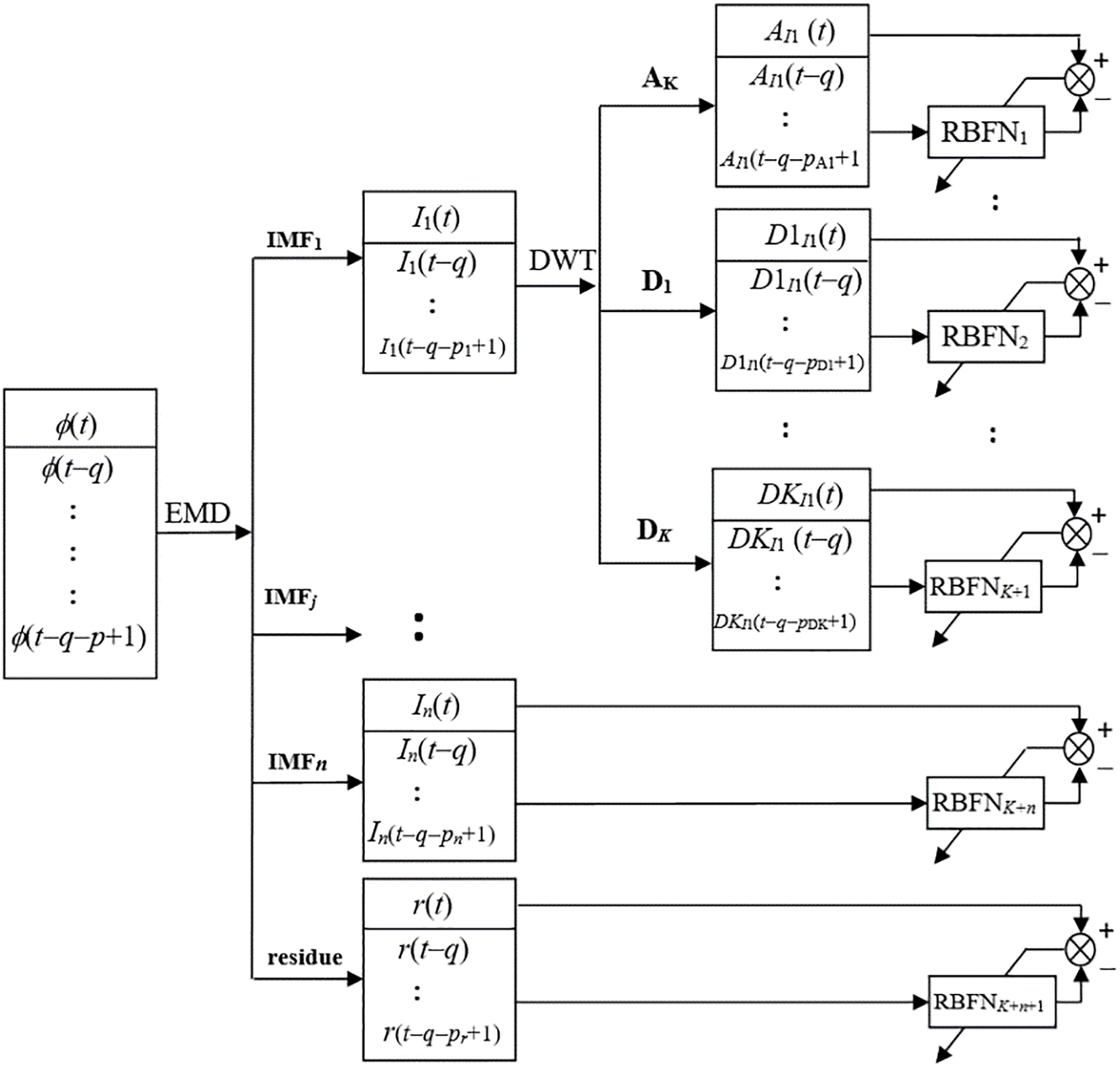
Identification procedure of the prediction scheme using EMD-DWT (q-steps-ahead).
During the identification process, variable networks are dynamically constructed for components generated by EMD and DWT in real time. In a sequential learning scheme, both processes of identification and prediction are carried out consecutively within each step with the prediction being executed immediately following the completion of the identification. The schematic of the prediction process is depicted in Figure 2.
Figure 2
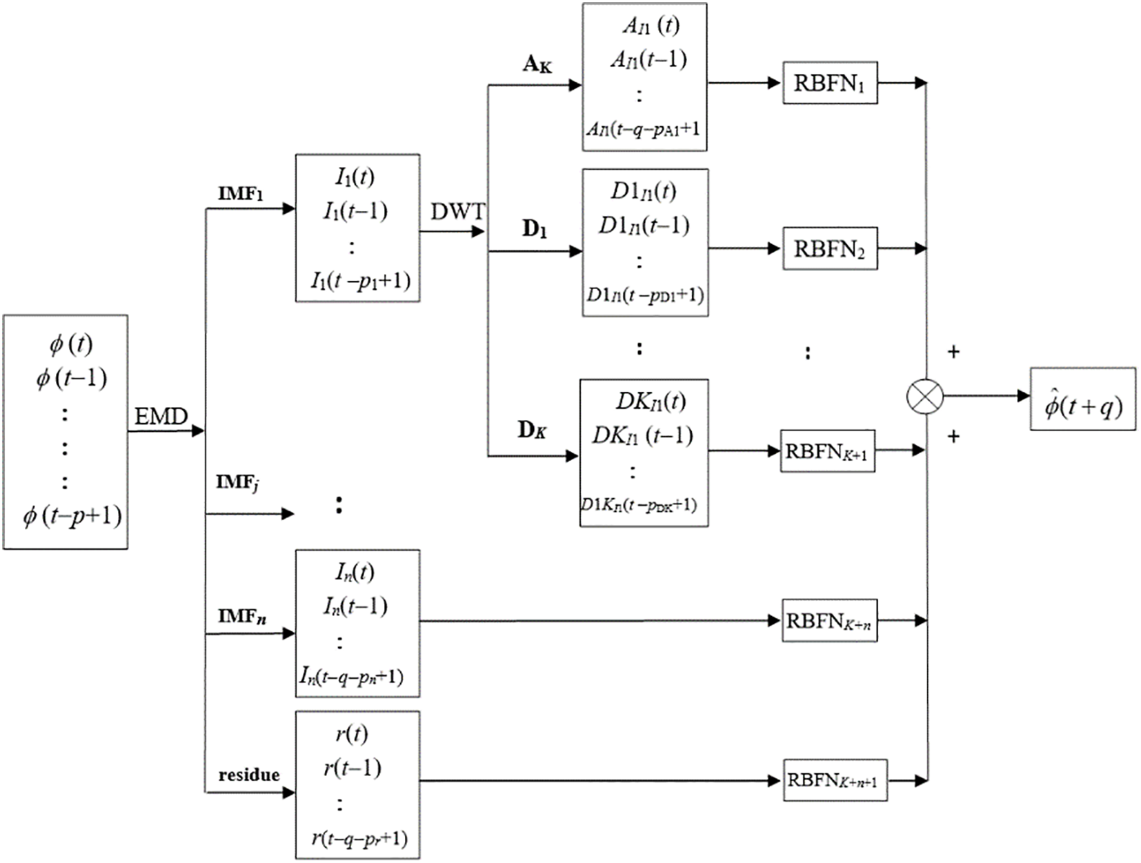
Prediction procedure based on EMD-DWT method.
The final prediction result is obtained by combining the prediction outputs of the individual IMFs and residue component, along with the detailed information and approximate information decomposed by the DWT.
4 Real-time tidal current prediction simulation
4.1 Simulation dataset
The data were sourced from the PORTS system of the United States National Oceanic and Atmospheric Administration (NOAA) to evaluate the effectiveness of the proposed mechanism. The tidal current station at Range A2, LB 29 Cumberland Sound (30°43.489’N, 81°29.067’W) is chosen as the target station for this study. Its near surface tidal current data were collected from July 1 GMT 0000, to Sept. 30 GMT 2359, 2024. This location was selected due to its position at the convergence of flows from Cumberland Sound, Cumberland Island Fry, St. Marys River, Beach Creek, and Jolly River, as depicted in Figure 3. In addition to hydrological and meteorological factors such as wind, air pressure, precipitation, and evaporation, the dynamics of tidal current at this site is also affected by the runoff flows, which add to the complexity of the tidal current variations.
Figure 3
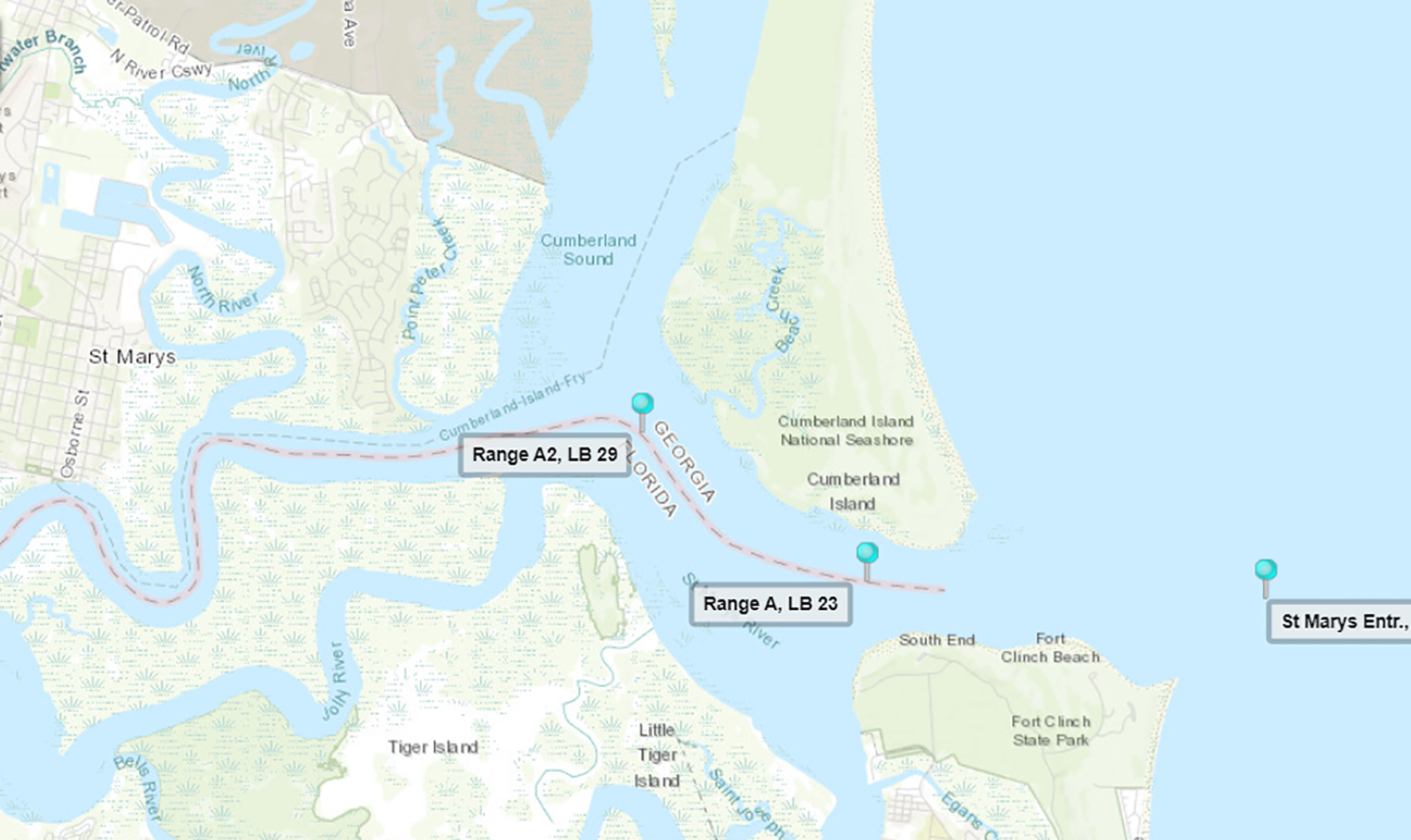
Location of the Cumberland sound (Source: https://tidesandcurrents.noaa.gov/).
The speed and direction of tidal current in Cumberland Sound are illustrated in Figure 4 and Figure 5, respectively. It is clearly shown in Figure 4 that the tidal speed displays periodic characteristics, and the tidal current direction also exhibits clustering effects at certain thresholds, as shown in Figure 5. To establish an appropriate prediction model, the tidal current was analyzed, and the statistical histogram based on the tidal current direction measurements from the Cumberland Sound station in 2022 is presented in Figure 6.
Figure 4
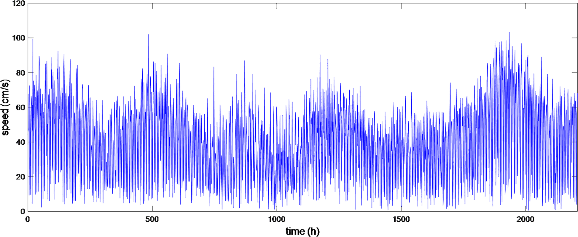
Tidal current speed of Cumberland sound.
Figure 5
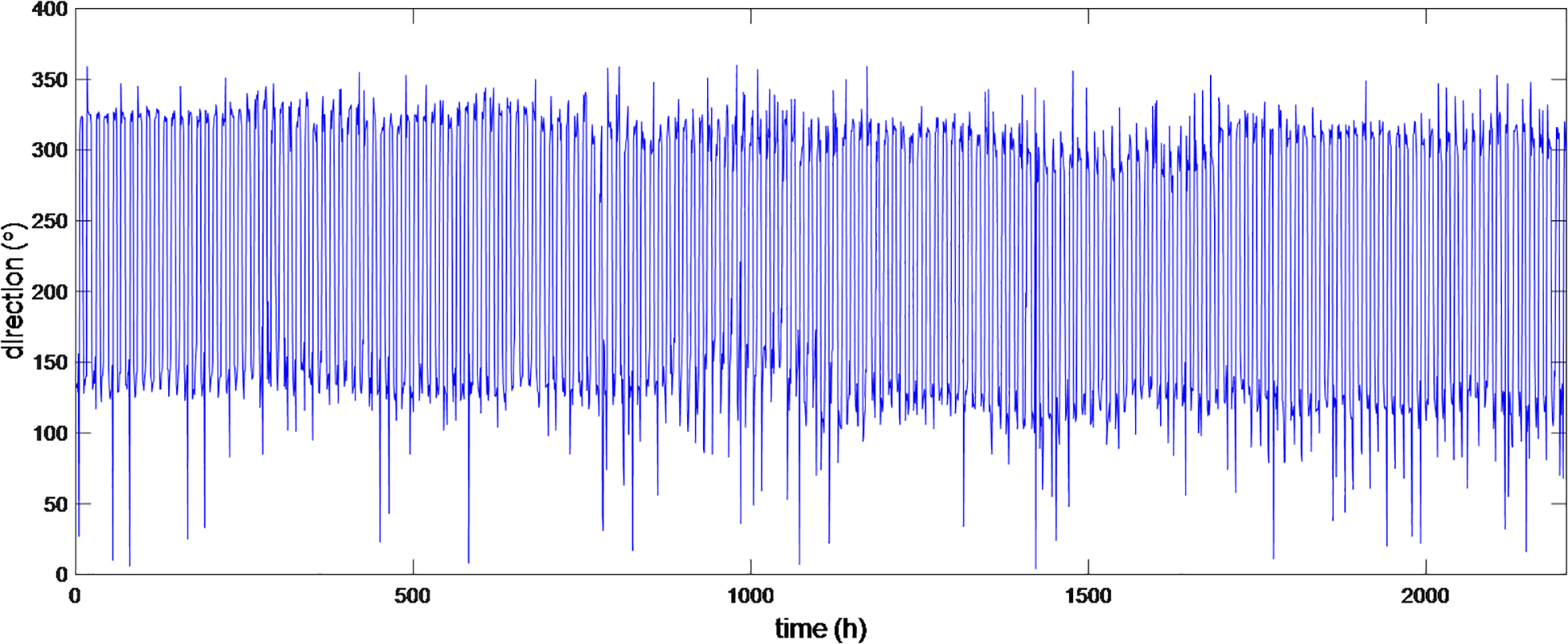
Tidal current direction of Cumberland sound.
Figure 6
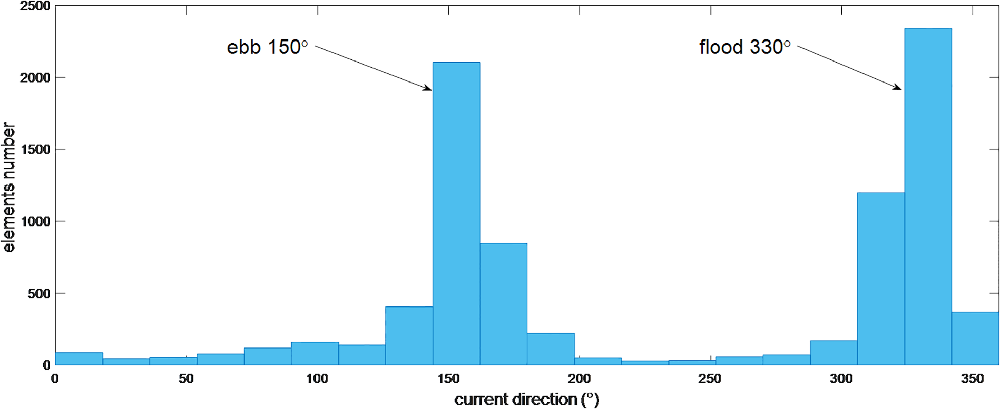
Statistics histogram of tidal current direction.
As depicted in Figure 6, the current exhibits a typical reciprocal pattern with a flood direction of 330° and an ebb direction of 150°. Consequently, to align with the needs of tidal power, the current measurements are represented and predicted as longitudinal current along 330° and lateral current along 60°. The current speeds along the longitudinal and lateral directions are illustrated in Figures 7 and 8, respectively.
Figure 7
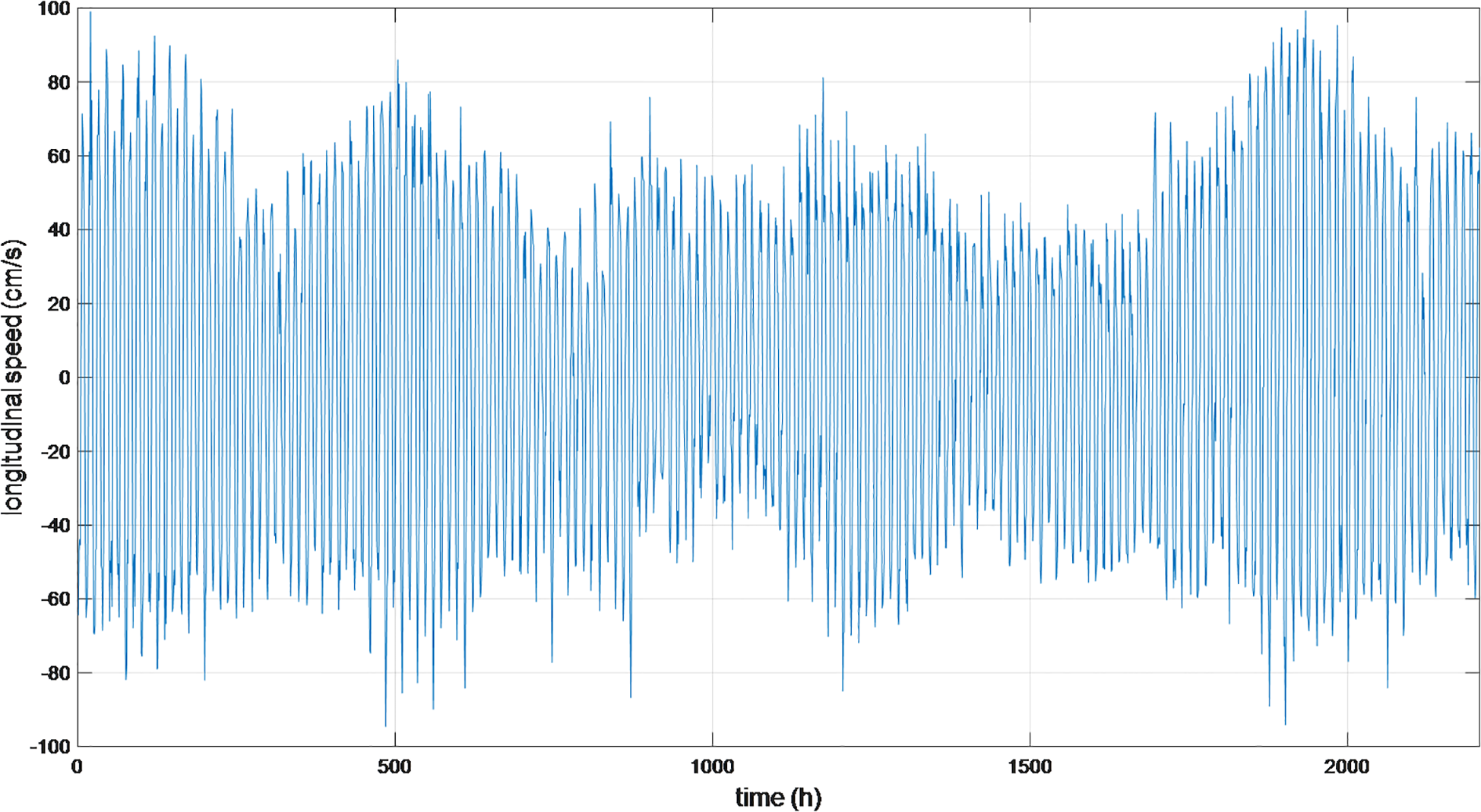
Longitudinal speed of tidal current of Cumberland sound (July 1 to Sept. 30, 2024).
Figure 8
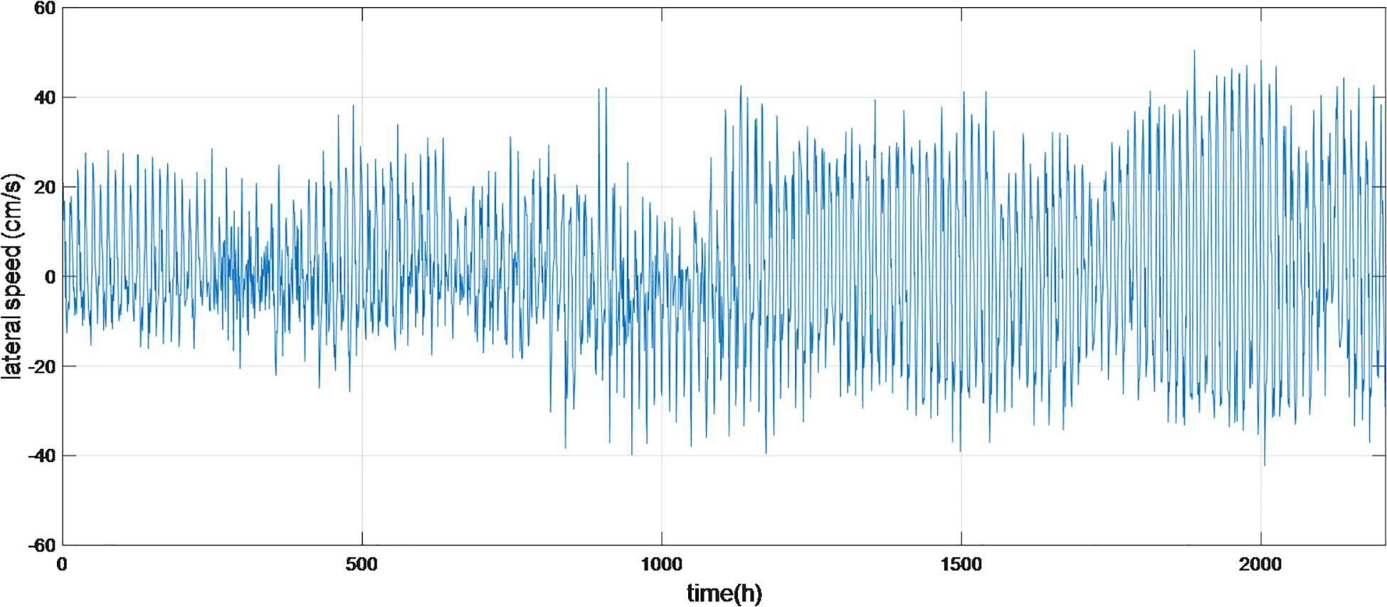
Lateral speed of tidal current of Cumberland sound (July 1 to Sept. 30, 2024).
It is demonstrated in Figures 7 and 8 that the variations of longitudinal and lateral currents are complex processes, posing challenges for identification and prediction. A single-step-ahead prediction experiment was conducted for 2000 steps with a time interval of 1 hour. The experiments were performed under Win10 system using computation platform of MATLAB R2009b, with the computation configuration of 11th Gen Intel(R) Core(TM) i7-1165G7 and the CPU at dual 2.80 GHz and RAM of 16.0 GB memory. The predictive efficacy of the proposed framework is assessed utilizing the quantitative metrics of root mean square error (RMSE)and the correlation coefficient (CC). The mathematical principle of the root mean square error is as shown in Equation 24
where y(t+q) and (t+q) represent the measured tidal current velocity and predicted ones at time of t+q, respectively.
The variations of tidal current can be attributed to the complex influences of external and internal factors. The EMD method is used to dissect the original signal into a series of components of IMFs which possess respective homogenous features. Initially, only the EMD decomposition was applied, resulting in the adaptive decomposition of 8 IMFs and 1 residual component, as shown in Figure 9.
Figure 9
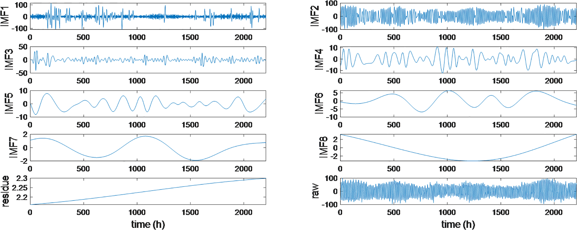
Decomposition of longitudinal speed by EMD.
It is illustrated in Figure 9 that the EMD decomposition can determine the order of decomposition automatically and transform non-stationary time series to substantially stationary signals. Moreover, obtaining a series of IMF components with distinct features can aid in revealing hidden mechanistic features within the time series, as an individual IMF component may explain a specific practical process.
Adaptive networks are utilized to predict individual IMFs in real time, and the Lipschitz quotients approach serves to ascertain the number of input variables for the neural predictive model. Consequently, the model input orders are determined for individual IMFs and the residual using the Lipschitz quotients approach, as illustrated in Figure 10.
Figure 10
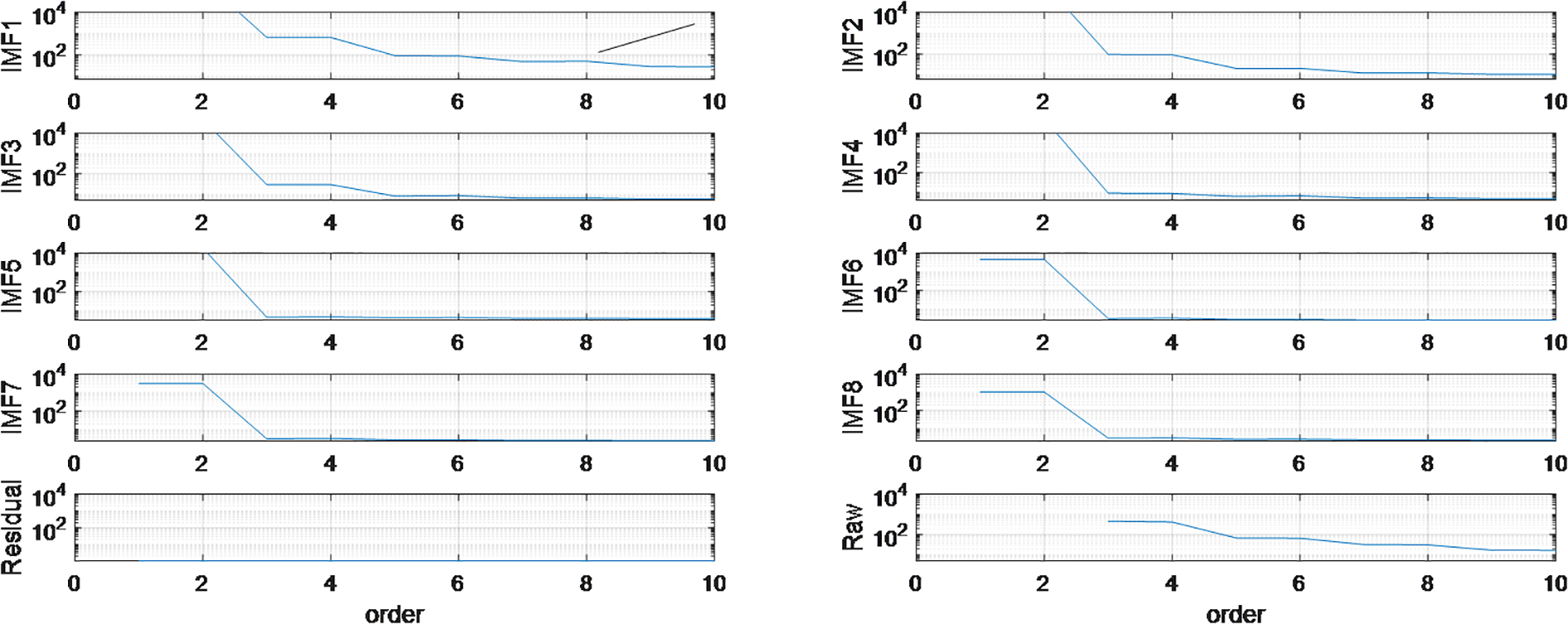
The Lipschitz quotients for IMFs and residual components of longitudinal current.
It is noticed in Figure 10 that in determining the Lipschitz quotients values corresponding to IMF1∼ IMF8, the quotients at order 3 q(3) are significantly declined compared to those at order 2 q(2); moreover, the corresponding q(4) exhibits only a marginal difference from q(3). Consequently, for components of IMF1∼ IMF8, the prediction model input orders are set as 3. The model input order for residual component cannot be determined using the Lipschitz quotients method directly, and it is set to 3 attributing to its approximately linear characteristics. For the residual component, the model input order cannot be explicitly decided via the Lipschitz quotients approach. Owing to its near-linear nature, the order is set to 3 consequently. For neural prediction in multi steps ahead, the input order are determined in a similar manner.
4.2 EMD-based neural network prediction
Since the data within each IMF exhibit homogeneous characteristics, individual networks are utilized for each IMF. The real-time tidal current prediction experiment for one step ahead is conducted with variable-structure networks being constructed and adjusted sequentially based on GOMS algorithm. The variable neural networks are utilized for all decomposed components, and the overall prediction results are sum of individual prediction results. The overall prediction result is depicted in Figure 11.
Figure 11
Neural prediction result for longitudinal speed result based on EMD decomposition.
The index of RMSE for the longitudinal tidal current prediction experiment is 9.412990 cm/s over 2000 steps. The prediction results align closely with the measured ones, exhibiting a CC of 0.976348, as depicted in Figure 12.
Figure 12
Prediction scatter diagram for longitudinal speed result based on EMD decomposition.
It is indicated from Figures 11 and 12 that the prediction results for longitudinal tidal speed can accurately track the variations of the real-measured data. Results exhibit the satisfactory holistic agreement of predicted longitudinal tidal speed with measured ones, demonstrating the adaptability of the proposed prediction strategy.
Data-driven techniques, such as neural networks, are extensively employed for handling complex systems due to their merits such as inherent nonlinearity and adaptability. Attributing to the inherent data-driven nature, the generalization ability of the neural network is significantly influenced by the complexity underlying samples. To optimize the data space thus alleviate the computation burden, the EMD method is firstly utilized to transforms the original time series into subseries with homogenous natures, which reduces the identification burden for the identification and enhances the efficiency of the neural prediction scheme.
Variable-structure neural networks are established and adjusted sequentially for individual components to accommodate their specific features. The prediction results for the components are presented in Figure 13, respectively.
Figure 13
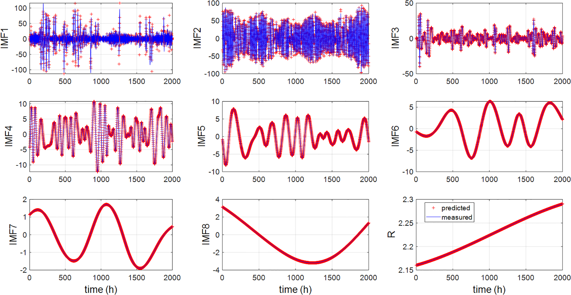
Prediction results for components by using the EMD-based neural prediction model.
It is noticed that the predicted values for IMFs 2-8 exhibit minimal deviations from the actual ones, indicating that the neural network with variable structure can effectively identify the time-varying dynamics of these components and produce accurate predictions. For the component of IMF1, the predicted values predominantly fall within the envelope curve of the original IMF1 signal, as further illustrated in Figure 14.
Figure 14
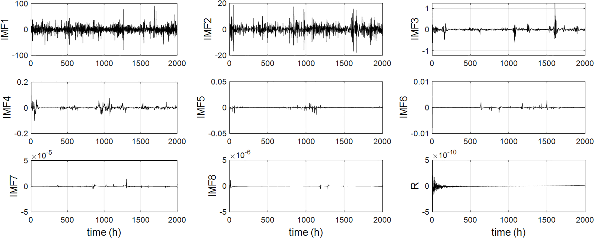
Prediction errors for components by using the EMD-based neural prediction model.
Significant deviation occurs in the prediction result of IMF1, with the index of RMSE reaching 8.5459 cm/s over 2000 steps. This is relatively high compared to the overall prediction errors. This discrepancy may be attributed to the presence of highly noisy signals and other unmodeled dynamics within the IMF1 component. Additionally, the decomposed IMF1 component contains signals with varying frequencies and amplitudes, which complicates prediction and degrades the performance of neural prediction approaches.
The improve the generalization ability of the neural networks, the networks are tuned not only in the parameters but also in the number of hidden units and their locations. For each IMF, the evolution history of hidden units’ number is depicted in Figure 15.
Figure 15
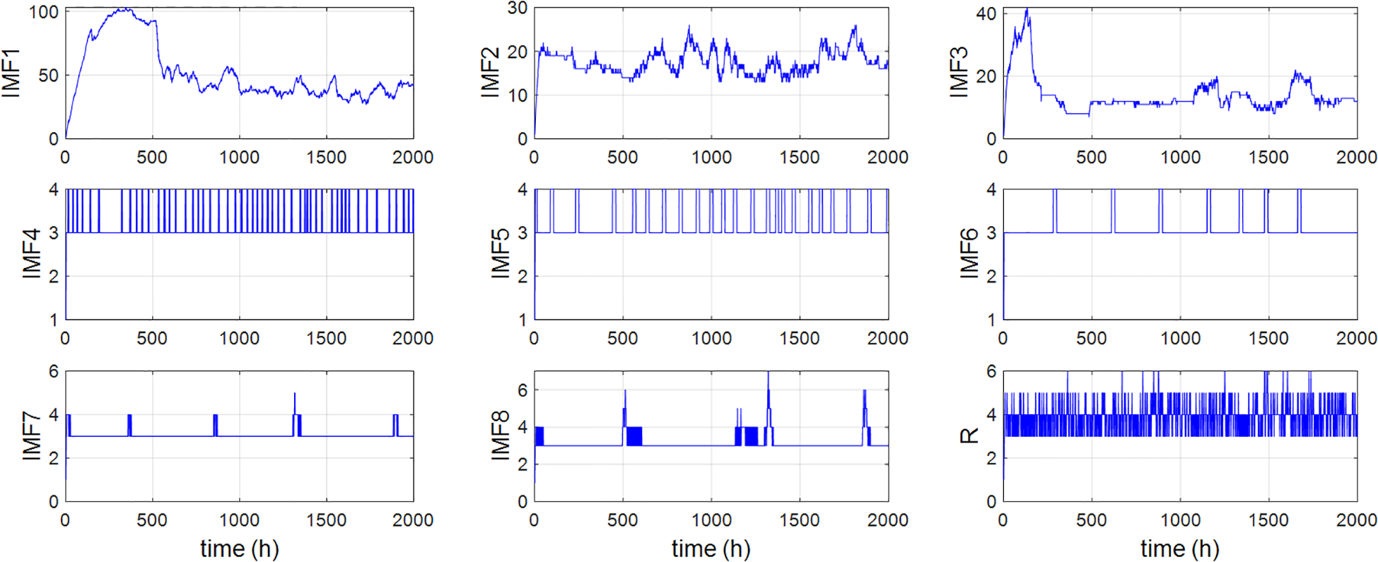
Evolution of hidden units number by the EMD-based neural prediction.
It is shown in Figure 15 that there exist vibrations at the initial stage of curves. This is because that the GOMS algorithm constructs the variable RBF network sequentially, starting from an empty network with no hidden units. The initial few samples in SDW are employed to construct hidden layer directly, then the hidden units are adjusted sequentially through the identification process. The number of hidden units (HUN) is variant, indicating that the hidden units are dynamically adjusted according to the identification of the time-varying SDW.
The total time consumed for 2000 steps is 26.6018 seconds, which is considerably fast because that only the samples within the SDW are processed. Despite the need to process 8 IMFs and 1 residual component, the fast processing speed, along with the adaptive determination of the EMD decomposition order and model input order, facilitates the practical online application of the prediction scheme.
4.3 Hierarchical EMD-SDW-based neural prediction scheme
It is indicated from Figures 13 and 14 that the prediction error decreases from IMF1 to IMF7 and to residual series. This trend can be attributed to the reduction in complexity and energy, which in turn simplifies the identification and prediction processes. The energy of the tidal current time series is predominantly concentrated in the first few IMFs, which also contribute significantly to the overall prediction error. To enhance prediction accuracy, one approach is to optimize the data structure in the time series of IMF1, thereby reducing the prediction burden. Therefore, in this study, the high-frequency component of IMF1 is further decomposed by using the DWT algorithm. The DWT decomposition order is set to 1 for simplicity, t, and ‘db4’ wavelet is used as the basis. The Lipschitz quotients method is employed to determine the model input orders for both the approximation and detail components, with both orders set to 3 for the predictions.
The resulting detail and approximation components are utilized for prediction, and the prediction outputs for all decomposed components are aggregated to produce the final prediction. The prediction results and the corresponding errors are illustrated in Figure 16.
Figure 16
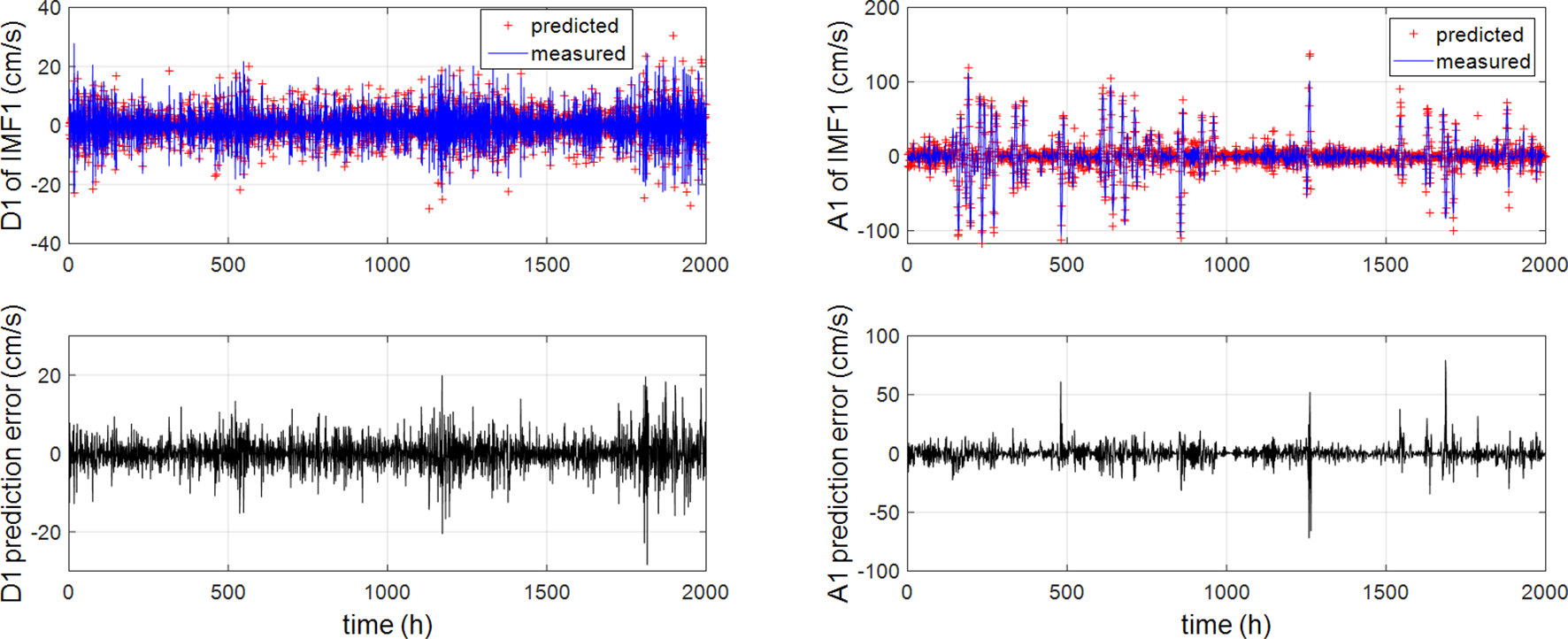
Prediction results by the proposed EMD-DWT-based neural prediction model.
It is shown in Figure 16 that the frequency aliasing is mitigated through the DWT decomposition. The prediction results show a good overall agreement with the tidal current measurements, indicating that the proposed prediction scheme based on hierarchical multi-stage decomposition can serve as a feasible approach for forecasting current profiles in strait areas.
The detail component contains a signal that resembles noise, while the approximation component exhibits a certain degree of regularity. The DWT decomposes IMF1 into two components, each with a homogeneous nature, which facilitates prediction using the neural model. The evolution history of the hidden units’ number during the prediction for the detail and approximation components of IMF1 are illustrated in Figure 17.
Figure 17
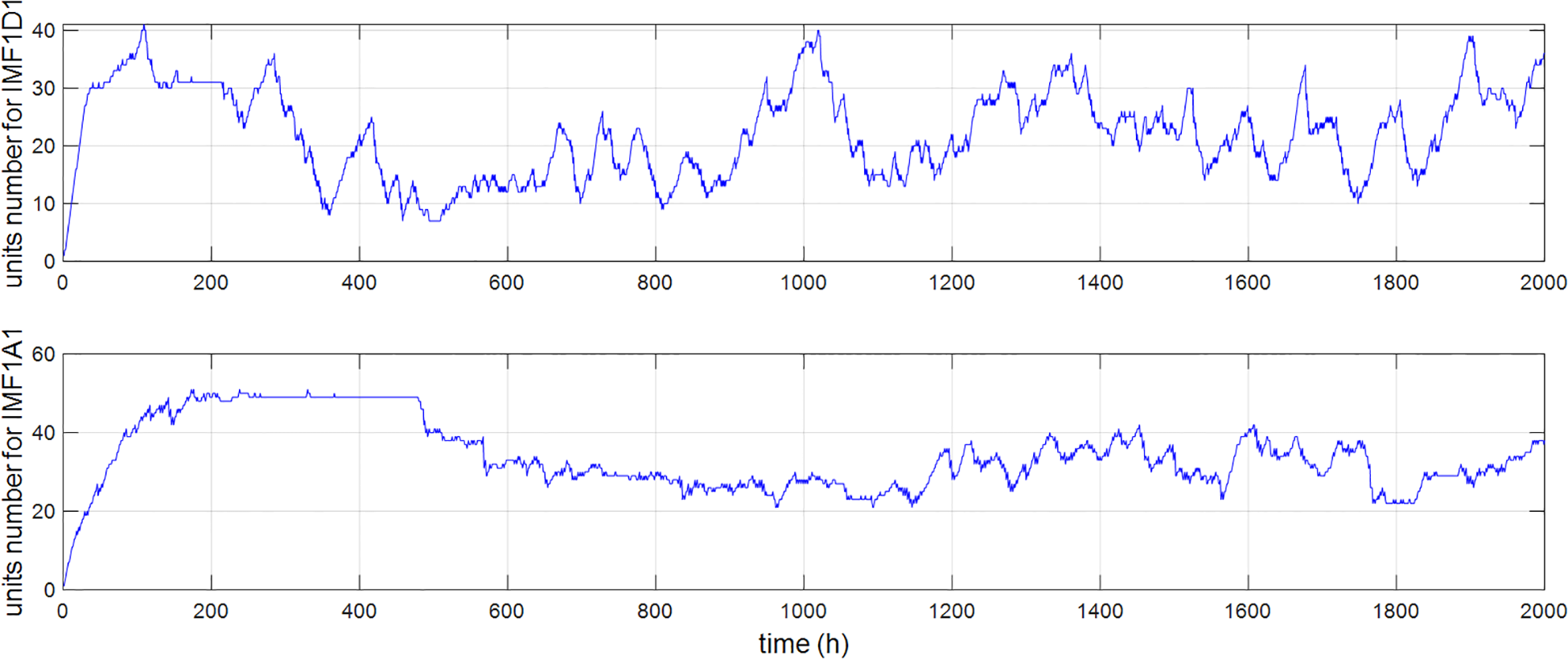
Evolution of hidden units’ number for detail and approximation components.
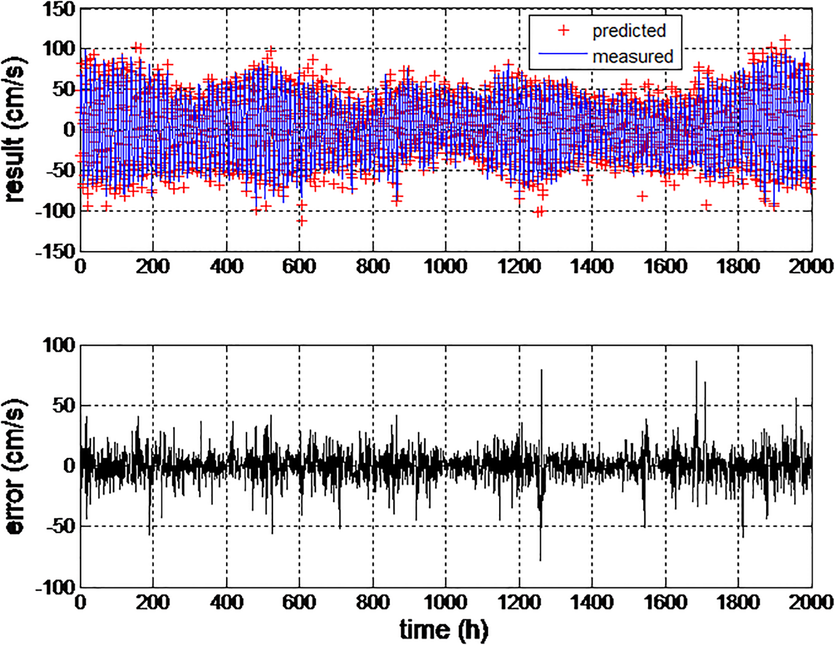
The predictions for the approximation and detail components are summed to generate the prediction of IMF1. This prediction is then added to the predictions of the other IMFs to obtain the overall longitudinal tidal current prediction. The overall prediction generated by the hierarchical EMD-DWT-based neural prediction scheme is depicted in Figure 18.
Figure 18
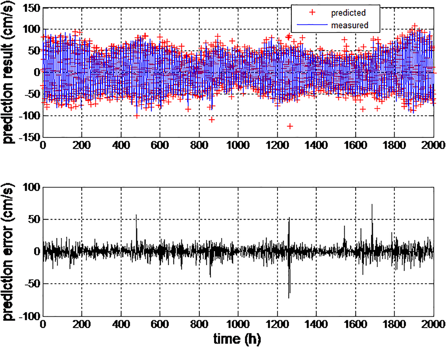
Prediction result by the EMD-DWT-based prediction.
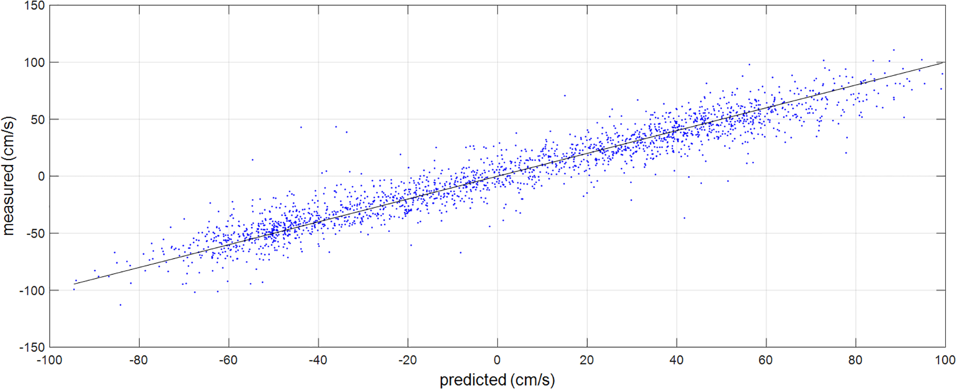
It is evident that the predicted longitudinal speed of the tidal current closely aligns with the actual measurements. The prediction RMSE has decreased to 8.886484 cm/s compared to the 9.412990 cm/s using the EMD-based prediction scheme. This reduction demonstrates the enhanced prediction accuracy of the EMD-DWT-based prediction configuration. The prediction results closely match the measured values, with a correlation coefficient of 0.978893, as illustrated in Figure 19.
Figure 19
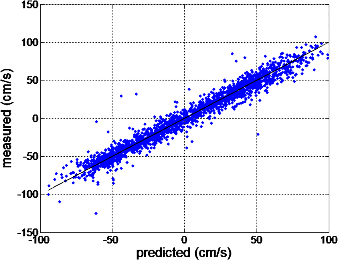
Scatter diagram based on hierarchical decomposition.
To evaluate the efficacy of the proposed scheme over an extended temporal spectrum, simulations were also conducted for various prediction lead times, and the prediction results are presented in Table 1.
Table 1
| Schemes | EMD-DWT | EMD | ||||
|---|---|---|---|---|---|---|
| lead time | RMSEPre (cm/s) | CC | time/step (s) | RMSEPre (cm/s) | CC | time/step (s) |
| 1 hour | 8.8865 | 0.9789 | 0.01331 | 9.4130 | 0.9763 | 0.01319 |
| 6 hours | 9.2483 | 0.9771 | 0.01522 | 11.656 | 0.9631 | 0.01427 |
| 12 hours | 10.4601 | 0.9706 | 0.01700 | 12.866 | 0.9554 | 0.01128 |
| 24 hours | 10.7163 | 0.9691 | 0.01971 | 13.1110 | 0.9532 | 0.01760 |
| 48 hours | 11.6365 | 0.9638 | 1.00152 | 13.4795 | 0.9505 | 0.01943 |
Prediction results for longitudinal tidal current.
It can be noticed from Table 1 that the prediction accuracy decreases as the increase of the prediction lead time. This is because that the prediction is generated based on the temporal data in the sliding window, which make the approach suitable for short-term predictions of time-varying systems.
As the tidal current incorporates the longitudinal and lateral current, its lateral part is also predicted with the prediction approaches based on decomposition parts of EMD and EMD-DWT, and the results are depicted in Table 2.
Table 2
| Schemes | EMD-DWT | EMD | ||||
|---|---|---|---|---|---|---|
| lead time | RMSEPre (cm/s) | CC | time/step (s) | RMSEPre (cm/s) | CC | time/step (s) |
| 1 hour | 5.8491 | 0.9388 | 0.01837 | 6.5685 | 0.9202 | 0.01122 |
| 6 hours | 7.0200 | 0.9091 | 0.02210 | 8.8865 | 0.9789 | 0.01760 |
| 12 hours | 7.3738 | 0.8984 | 0.02214 | 9.6604 | 0.8185 | 0.01625 |
| 24 hours | 9.4130 | 0.9763 | 0.01997 | 10.025 | 0.8027 | 0.10217 |
| 48 hours | 10.71623 | 0.9691 | 0.01839 | 11.656 | 0.9631 | 0.01327 |
Prediction results for lateral tidal current.
It is evident that the EMD-DWT-based neural prediction scheme produces relatively stable predictions for lead times ranging from 1 hour to 48 hours. This stability can be a result of the hierarchical multi-stage decomposition strategy, which optimize the data space and converts the original tidal current time series into more detailed multi-resolution subseries with homogeneous characteristics. This alleviate the system identification burden by using variable neural networks. Generally, prediction accuracy decreases as the lead time increases, showing the existence of time-varying dynamics of tidal currents. The scheme’s computation speed is considerably fast because the variable network’s learning scheme processes only a limited number of samples in the SDW, comparing to the entire dataset in a batch learning strategy. This merit also facilitates the practical applications in real time of the proposed scheme.
The comparison validated the satisfactory overall performance of the EMD-DWT-based neural model with respect to prediction accuracy and processing speed. The design of the SDW enables fast processing and adaptability to time-varying dynamics, while the EMD-DWT transform ensures the accuracy and reliability of the predictions. The hierarchical-decomposition-based sequential prediction scheme offers a potential solution for online identification and prediction of a set of complex systems.
5 Conclusion
To accurately model the complex characteristics of tidal currents, which are influenced by environmental disturbances, an adaptive tidal current prediction scheme based on hierarchical decomposition is proposed. This scheme ensembles hierarchical multi-resolution decomposition techniques with a variable RBF network. The coefficients of decomposition order and the model input order of the neural prediction model are both autonomously decided by the approaches of EMD composition and the Lipschitz quotients algorithm, respectively. To alleviate the computational burdens of identification of complex processes, the tidal current time series is hierarchically decomposed into a set of IMFs, with the highest-energy IMF1 being further decomposed using the DWT decomposition. The achieved components from hierarchical decomposition are identified by the variable RBF network. The overall tidal current prediction is obtained by recombining the predicted values of the IMFs from EMD, as well as the detail and approximation components from DWT. Simulations of real-time tidal current prediction were performed and the results validate the viability and efficacy of the proposed prediction framework, featured by its high precision and rapid computational efficiency. The self-adaptive nature of the prediction framework coefficients enhances its practical feasibility. By analyzing the potential physical significance of different IMF or DWT components in relation to coastal ocean dynamics would improve the transparency and interpretability of the model outputs. However, the proposed strategy is driven by the data in the SDW and is hard to capture the long-term system variations. Our future research work will focus on the insight of the interpretability of the hierarchically decomposed components as well as the combination with mechanism model of tidal current variations with long-term dynamic tidal current features.
Statements
Data availability statement
The original contributions presented in the study are included in the article/supplementary material. Further inquiries can be directed to the corresponding author.
Author contributions
NW: Conceptualization, Data curation, Formal Analysis, Funding acquisition, Investigation, Methodology, Project administration, Resources, Software, Supervision, Validation, Visualization, Writing – original draft, Writing – review & editing.
Funding
The author(s) declare that financial support was received for the research and/or publication of this article. This work was supported by the National Natural Science Foundation of China under Grants 52271361 and 52231014, the Special Projects of Key Areas for Colleges and Universities in Guangdong Province under Grant 2021ZDZX1008, the Natural Science Foundation of Guangdong Province of China under Grant 2023A1515010684, and the Program for Scientific Research Start-Up Funds of Guangdong Ocean University.
Conflict of interest
The author declares that the research was conducted in the absence of any commercial or financial relationships that could be construed as a potential conflict of interest.
Generative AI statement
The author(s) declare that no Generative AI was used in the creation of this manuscript.
Any alternative text (alt text) provided alongside figures in this article has been generated by Frontiers with the support of artificial intelligence and reasonable efforts have been made to ensure accuracy, including review by the authors wherever possible. If you identify any issues, please contact us.
Publisher’s note
All claims expressed in this article are solely those of the authors and do not necessarily represent those of their affiliated organizations, or those of the publisher, the editors and the reviewers. Any product that may be evaluated in this article, or claim that may be made by its manufacturer, is not guaranteed or endorsed by the publisher.
References
1
Almunif A. Fan L. Miao Z. (2020). A tutorial on data-driven eigenvalue identification: Prony analysis, matrix pencil, and eigensystem realization algorithm. Int. Trans. Electr. Energy Syst.30, 12283. doi: 10.1002/2050-7038.12283
2
Aly H. H. H. (2020a). Intelligent optimized deep learning hybrid models of neuro wavelet, Fourier Series and Recurrent Kalman Filter for tidal currents constitutions forecasting. Ocean Eng.218, 108254. doi: 10.1016/j.oceaneng.2020.108254
3
Aly H. H. H. (2020b). A novel approach for harmonic tidal currents constitutions forecasting using hybrid intelligent models based on clustering methodologies. Renew. Energy147, 1554–1564. doi: 10.1016/j.renene.2019.09.107
4
Aydog B. Ayat B. Öztürk M. N. (2010). Current velocity forecasting in straits with artificial neural networks, a case study: Strait of Istanbul. Ocean Eng.37, 443–453. doi: 10.1016/j.oceaneng.2010.01.016
5
Bradbury M. C. Conley D. C. (2021). Using artificial neural networks for the estimation of subsurface tidal currents from high-frequency radar surface current measurements. Remote Sens.13, 3896. doi: 10.3390/rs13193896
6
Chang Y. C. Tseng R. S. Chen G. Y. (2013). Ship routing utilizing strong ocean currents. J. Navig.66, 825–835. doi: 10.1017/S0373463313000441
7
Chen S. Chng E. S. Alkadhimi K. (1991). Orthogonal least squares learning algorithm for radial basis function networks. IEEE Trans. Neural Netw.64, 829–837. doi: 10.1109/72.80341
8
Chen H. Li Q. Benbouzid M. (2021). Development and research status of tidal current power generation systems in China. J. Mar. Sci. Eng.9, 1286. doi: 10.3390/jmse9111286
9
Davidson F. J. M. Allen A. Brassington G. B. (2009). Applications of GODAE ocean current forecasts to search and rescue and ship routing. Oceanography22, 176–181. doi: 10.5670/oceanog.2009.76
10
Feil B. Abonyi J. Szeifert F. (2004). Model order selection of nonlinear input–output models—-a clustering based approach. J. Process Control14, 593–602. doi: 10.1016/j.jprocont.2004.01.005
11
Feng S. W. Chai K. (2020). An improved method for EMD modal aliasing effect. Vibroeng. Proc.35, 76–81. doi: 10.21595/vp.2020.21778
12
He X. Asada H. (1993). “A new method for identifying orders of input-output models for nonlinear dynamic systems,” in Proc. IEEE 1993 Am. Control Conf. 2520–2523.
13
Hong L. Li H. Peng K. (2021). A combined radial basis function and adaptive sequential sampling method for structural reliability analysis. Appl. Math. Modell.90, 375–393. doi: 10.1016/j.apm.2020.08.042
14
Hu Z. Li H. Wang D. (2023). Characterizing tidal currents and Guangdong coastal current over the northern South China Sea shelf using Himawari-8 geostationary satellite observations. Earth Space Sci.10, e2023EA003047. doi: 10.1029/2023EA003047
15
Huang C. Li Y. Yao X. (2019). A survey of automatic parameter tuning methods for metaheuristics. IEEE Trans. Evol. Comput.24, 201–216. doi: 10.1109/TEVC.4235
16
Huang Z. Xu H. Bai Y. (2023). Coastline changes and tidal current responses due to the large-scale reclamations in the Bohai Bay. J. Oceanol. Limnol.41, 2045–2059. doi: 10.1007/s00343-022-2235-6
17
Huang B. G. Zou Z. J. Ding W. W. (2018). Online prediction of ship roll motion based on a coarse and fine tuning fixed grid wavelet network. Ocean Eng.160, 425–437. doi: 10.1016/j.oceaneng.2018.04.065
18
Jahromi M. Maswood A. I. Tseng K. J. (2010). Long term prediction of tidal currents. IEEE Syst. J.5, 146–155. doi: 10.1109/JSYST.2010.2090401
19
Jalali S. M. J. Ahmadian S. Noman M. K. Khosravi A. Islam S. M.S. Wang F. et al (2022). Novel uncertainty-aware deep neuroevolution algorithm to quantify tidal forecasting. IEEE Trans. Ind. Appl.58, 3324–3332. doi: 10.1109/TIA.2022.3162186
20
Jin G. Pan H. Zhang Q. Zhang Y. Dong X. Wang Y. et al . (2018). Determination of harmonic parameters with temporal variations: An enhanced harmonic analysis algorithm and application to internal tidal currents in the South China Sea. J. Atmos. Oceanic Technol.35, 1375–1398. doi: 10.1175/JTECH-D-16-0239.1
21
Kavousi-Fard A. (2016). A hybrid accurate model for tidal current prediction. IEEE Trans. Geosci. Remote Sens.55, 112–118. doi: 10.1109/TGRS.2016.2596320
22
Kavousi-Fard A. (2017). A novel probabilistic method to model the uncertainty of tidal prediction. IEEE Trans. Geosci. Remote Sens.55, 828–833. doi: 10.1109/TGRS.2016.2615687
23
Kavousi-Fard A. Su W. (2017). A combined prognostic model based on machine learning for tidal current prediction. IEEE Trans. Geosci. Remote Sens.55, 3108–3114. doi: 10.1109/TGRS.2017.2659538
24
Kumar V. S. Kumar K. A. (2010). Waves and currents in tide-dominated location off Dahej, Gulf of Khambhat, India. Mar. Geod.33, 218–231. doi: 10.1080/01490419.2010.492299
25
Li B. Wang Y. Wei Z. Pan H. Xu T. Lv X. et al (2023). Changing the unpredictable nature of internal tides through deep learning. Geophys. Res. Lett.50, e2022GL102227. doi: 10.1029/2022GL102227
26
Li L. Wu W. Zhang W. Zhu Z. Li Z. Wang Y. et al . (2023). Storm surge level prediction based on improved NARX neural network. J. Comput. Electron.22, 783–804. doi: 10.1007/s10825-023-02005-z
27
Li G. Zhu W. (2023). Tidal current energy harvesting technologies: A review of current status and life cycle assessment. Renew. Sustain. Energy Rev.179, 113269. doi: 10.1016/j.rser.2023.113269
28
Liu X. Chen Z. Si Y. Qian P. Wu H. Cui L. et al . (2021). A review of tidal current energy resource assessment in China. Renew. Sustain. Energy Rev.145, 111012. doi: 10.1016/j.rser.2021.111012
29
Liu H. Mi X. Li Y. (2018). Smart deep learning based wind speed prediction model using wavelet packet decomposition, convolutional neural network and convolutional long short term memory network. Energy Convers. Manage.166, 120–131. doi: 10.1016/j.enconman.2018.04.021
30
Liu X. Yuan D. Wang X. (2023). Discussion on the method for tidal current quasi-harmonic analysis. Coast. Eng.42, 88–98. doi: 10.12362/j.issn.1002-3682.20220302001
31
Mishra R. K. Reddy G. S. Pathak H. (2021). The understanding of deep learning: A comprehensive review. Math. Probl. Eng.1, 5548884. doi: 10.1155/2021/5548884
32
Özger M. Başakın E. E. Ekmekcioğlu Ö. (2020). Comparison of wavelet and empirical mode decomposition hybrid models in drought prediction. Comput. Electron. Agric.179, 105851. doi: 10.1016/j.compag.2020.105851
33
Qian P. Feng B. Liu X. Zhang D. Yang J. Ying Y. et al . (2022). Tidal current prediction based on a hybrid machine learning method. Ocean Eng.260, 111985. doi: 10.1016/j.oceaneng.2022.111985
34
Qiao X. Guo F. Zhang R. (2020). “Short-term tidal current prediction based on GA-BP neural network,” in IOP Conf. Ser.: Earth Environ. Sci, vol. 513. (IOP Publishing), 012061.
35
Remya P. G. Kumar R. Basu S. (2012). Forecasting tidal currents from tidal levels using genetic algorithm. Ocean Eng.40, 62–68. doi: 10.1016/j.oceaneng.2011.12.002
36
Sarkar D. Osborne M. A. Adcock T. A. A. (2019). Spatiotemporal prediction of tidal currents using Gaussian processes. J. Geophys. Res. Oceans124, 2697–2715. doi: 10.1029/2018JC014471
37
Schuman C. D. Birdwell J. D. (2013). Variable structure dynamic artificial neural networks. Biol. Inspired Cogn. Arch.6, 126–130. doi: 10.1016/j.bica.2013.05.001
38
Shu Y. Han B. Song L. Yan T. Gan L. Zhu Y. et al . (2024). Analyzing the spatio-temporal correlation between tide and ship behavior at estuarine port for energy-saving purposes. Appl. Energy367, 123382. doi: 10.1016/j.apenergy.2024.123382
39
Wallot S. Mønster D. (2018). Calculation of average mutual information (AMI) and false-nearest neighbors (FNN) for the estimation of embedding parameters of multidimensional time series in matlab. Front. Psychol.9, 1679. doi: 10.3389/fpsyg.2018.01679
40
Wang J. S. Chen Y. P. (2006). A fully automated recurrent neural network for unknown dynamic system identification and control. IEEE Trans. Circuits Syst. I Reg. Papers53, 1363–1372. doi: 10.1109/TCSI.2006.875186
41
Wang J. S. Hsu Y. L. Lin H. Y. (2009). Minimal model dimension/order determination algorithms for recurrent neural networks. Pattern Recognit. Lett.30, 812–819. doi: 10.1016/j.patrec.2008.05.007
42
Yin J. C. Perakis A. N. Wang N. (2018). A real-time ship roll motion prediction using wavelet transform and variable RBF network, “. Ocean Eng.vol, 10–19. doi: 10.1016/j.oceaneng.2018.04.058
43
Yin J. C. Wang N. N. Shu Y. Q. (2025). An adaptive real-time ship roll motion prediction scheme based on two-stage multi-resolution decomposition. Ocean Eng.325, 120741. doi: 10.1016/j.oceaneng.2025.120741
44
Zhang L. Duan W. Y. Cui X. M. (2024). Surface current prediction based on a physics-informed deep learning model. Appl. Ocean Res.148, 104005. doi: 10.1016/j.apor.2024.104005
45
Zhang A. Lin Y. Sun Y. Yuan H. Wang M. Liu G. et al . (2022). Tidal current prediction based on fractal theory and improved least squares support vector machine. IET Renew. Power Gener.16, 389–401. doi: 10.1049/rpg2.12335
46
Zhang K. Wang X. Wu H. Zhang X. Fang Y. Zhang L. et al . (2023). Study of the performance of deep learning methods used to predict tidal current movement. J. Mar. Sci. Eng.11, 26. doi: 10.3390/jmse11010026
47
Zhang Z. Zhang L. Yue S. (2023). Correction of nonstationary tidal prediction using deep-learning neural network models in tidal estuaries and rivers. J. Hydrology622, 129686. doi: 10.1016/j.jhydrol.2023.129686
Summary
Keywords
coastal current prediction, hierarchical decomposition, sequential learning, time series prediction, time series decomposition
Citation
Wang N (2025) A sequential coastal current prediction approach based on hierarchical decomposition. Front. Mar. Sci. 12:1668178. doi: 10.3389/fmars.2025.1668178
Received
17 July 2025
Accepted
19 August 2025
Published
09 September 2025
Volume
12 - 2025
Edited by
Chengbo Wang, University of Science and Technology of China, China
Reviewed by
Guoshuai Li, Dalian Maritime University, China
Xiaolie Wu, Wuhan University of Technology, China
Updates
Copyright
© 2025 Wang.
This is an open-access article distributed under the terms of the Creative Commons Attribution License (CC BY). The use, distribution or reproduction in other forums is permitted, provided the original author(s) and the copyright owner(s) are credited and that the original publication in this journal is cited, in accordance with accepted academic practice. No use, distribution or reproduction is permitted which does not comply with these terms.
*Correspondence: Nini Wang, wangnini@gdou.edu.cn
Disclaimer
All claims expressed in this article are solely those of the authors and do not necessarily represent those of their affiliated organizations, or those of the publisher, the editors and the reviewers. Any product that may be evaluated in this article or claim that may be made by its manufacturer is not guaranteed or endorsed by the publisher.