Abstract
The challenges of high computational complexity as well as the corresponding long time consumption are like the Achilles’ Heel in the traditional numerical methods for solving the large-scale underwater acoustic field. An efficient solution method for the parabolic equation model based on the Fourier Neural Operator was proposed in this work. This method enables efficient global feature extraction through spectral convolution, thereby effectively establishing robust correlations between physical field parameters and the target sound pressure field. A continuous mapping was constructed in this model, which ensures that this algorithm could effectively adapt to various marine scenarios through the self-adjustment function. Experimental results demonstrate that the model achieves an average coefficient of determination R2> 0.95 and a relative Root Mean Square Error (RMSE) < 0.04 dB in the predicted sound pressure field, which represents various complex ocean conditions, including the scenarios with non-uniform sound speed profiles, broadband sound sources, and sloped bathymetry, among others. Compared to the conventional RAM approach, the model proposed in this study achieves the equivalent accuracy while reducing the computational latency, with a demonstrated decrease ranging from 25% to 35%. This superior performance could be attributed to the adopted grid-independent O(nlogn) spectral convolution architecture. These results demonstrate the robustness and applicability of the framework, highlighting the potential for broader application in underwater sound field prediction in the future.
1 Introduction
The parabolic equation (PE) serves as a fundamental methodology for modeling underwater acoustic propagation. The computational efficiency of this approach derives from the far-field approximation of the Helmholtz equation (Ivansson, 2017; Collins and Dacol, 2000; Collins, 2012). However, time-varying sound speed profiles and complex seabed topography in real-world marine environments induce multipath interference effects. These effects pose three principal challenges to the conventional Split-Step Padé algorithm:(1) Strong coupling among iteration step size, grid resolution, and computational domain extent results in a cubic increase in computational complexity related to sea area scale; (2) The phase-sensitive characteristics of acoustic fields requires subwavelength-scale spatial discretization (Collins, 1993), which substantially increases the memory resource requirements; (3) The environmental parameter perturbations–particularly the sound velocity gradient variations of ±5%, require the regeneration of computational meshes, thereby constraining the real-time forecasting capabilities.
In response to the aforementioned computational challenges, machine learning approaches in the underwater acoustic field modeling have progressed through three stages of development. (Appendix Table A1 in Supplementary Material systematically outlines the three developmental stages of machine learning (ML)-driven underwater acoustic field modeling, serving as a critical technical backdrop to address the computational inefficiencies of conventional parabolic equation (PE) methods. For Traditional ML approaches (e.g., multilayer feedforward networks), they are rooted in Hornik’s Universal Approximation theorem, yet inherent grid dependency impairs their ability to accurately represent the acoustic field’s global coherent structure, limiting applications to simple scenarios (e.g., uniform sound speed, flat seabeds) (Hornik et al., 1989; Lagaris et al., 1998; Dissanayake and Phan-Thien, 1994; Berg and Nyström, 2018; Psichogios and Ungar, 1992; Hinze et al., 2009). Physics-Informed Neural Networks (PINNs) eliminate grid reliance by integrating wave equation constraints, but their high computational cost (requiring extensive iterations per scenario) and poor generalization restrict use in large-scale acoustic propagation simulations (Raissi et al., 2019; Du et al., 2023).In contrast, Neural Operators (with Fourier Neural Operator, FNO, as a representative) innovate via function-space mapping—establishing generalized links between environmental parameters (e.g., sound speed profiles) and acoustic solutions (e.g., sound pressure fields). Notably, FNO inherently aligns with acoustic wave propagation mechanisms through spectral convolution, making it advantageous for complex marine environments (Lu et al., 2021; Li et al., 2021).This table clarifies trade-offs among existing methods: Traditional ML and PINNs fail to balance accuracy, efficiency, and generalization for large-scale underwater acoustics, while FNO’s unique attributes highlight its potential to optimize PE solvers. This forms the core motivation for developing the FNO-enhanced PE framework in this study.
Data-driven agent models originate from Hornik’s 1989 theoretical foundation, which established multilayer feedforward networks as universal approximators (Hornik et al., 1989). Based on this foundation, subsequent studies developed neural network methodologies for approximating partial differential equations (PDEs) (Hornik et al., 1989; Lagaris et al., 1998; Dissanayake and Phan-Thien, 1994; Berg and Nyström, 2018; Psichogios and Ungar, 1992; Hinze et al., 2009). Among the notable approaches, Lagaris’ method (Lagaris et al., 1998), parametrizes PDE solutions directly through neural networks by constructing boundary-compliant initial solutions and embedding both governing equations and boundary conditions within the loss function during the optimization process. In contrast, Berg and Nyström (Berg and Nyström, 2018) employ the neural network forward propagation to generate solution predictions, utilizing gradient-based optimization to minimize residuals between predicted and reference solutions.
However, these pioneering methods are still limited by the high costs associated with generating training data and the inherent constraints posed by grid dependency.
Furthermore, these methods remain constrained by problem-specific assumptions and exhibit limited adaptability to complex marine environments characterized by abrupt bathymetry and heterogeneous sound speed fields. While effective for applications such as noise analysis and reverberation prediction, their computational efficiency in large-scale simulations remains unresolved.
Physics-Informed Neural Networks (PINNs) eliminate grid dependency via embedded PDE constraints but face limitations in underwater acoustics: high computational cost (> 103 iterations/scenario), poor generalization requiring retraining for new conditions, and noise sensitivity (2 dB error increase at 10% SNR). Although machine learning has advanced beyond grid dependency, the conflict between real-time prediction and large-scale computation persists. Neural operators overcome dimensional limitations by learning mappings between function spaces (Lu et al., 2021). Their key innovation lies in constructing generalized mappings from parameter spaces to solution spaces during a single training cycle, enabling solutions for entire PDE families and significantly enhancing generalization. Among these, the Fourier Neural Operator (FNO) achieves efficient global feature extraction via spectral convolution. This confers sublinear time complexity during evaluation, providing a foundation for large-scale underwater acoustic computations. As a spectral-domain framework, FNO excels in multidisciplinary modeling, demonstrating advantages in: (1) Accelerating physical field solutions (e.g (Sun et al., 2023; Zhu et al., 2021; Xiao et al., 2024; Du et al., 2023; Yoon et al., 2024; Xi et al., 2023)); (2) Data-driven parametric modeling substitutes (e.g (Zhong et al., 2023; Lake et al., 2024; Yin et al., 2024)); (3) Complex dynamical system modeling (e.g (Collins, 2012; Mangeleer and Louppe, 2023; Zhong et al., 2023)), combining multiscale capture with robust generalization. Empirical evidence consistently shows FNO accelerates computation while preserving accuracy, offering a novel paradigm for high-dimensional PDEs and the potential to supplant conventional methods. Nevertheless, FNO’s application to underwater acoustic parabolic equations remains unexplored.
This study establishes an FNO-based parabolic equation solver to address limitations in training data demands and generalization. The proposed framework maintains robust performance under variations in environmental parameters and source configurations.
Subsequent sections systematically detail the FNO-PE solver architecture (Section 2), multiphysics validation datasets and evaluation metrics (Section 2.5), comparative analyses with benchmark methods across diverse marine conditions (Section 3), and principal conclusions with prospective research directions (Section 4).
2 Methodology
This section presents the construction of deep networks through multi-input FNOs, introduces the PE formulation, and simulates the solution process based on FNO theory. The extended multi-input FNO architecture is subsequently analyzed.
2.1 Fourier neural operator
The neural operator is formulated as an iterative architecture (Zhang et al., 2022): , where vj, j = 0,1,…T-1 is a sequence of functions, each in the range of .
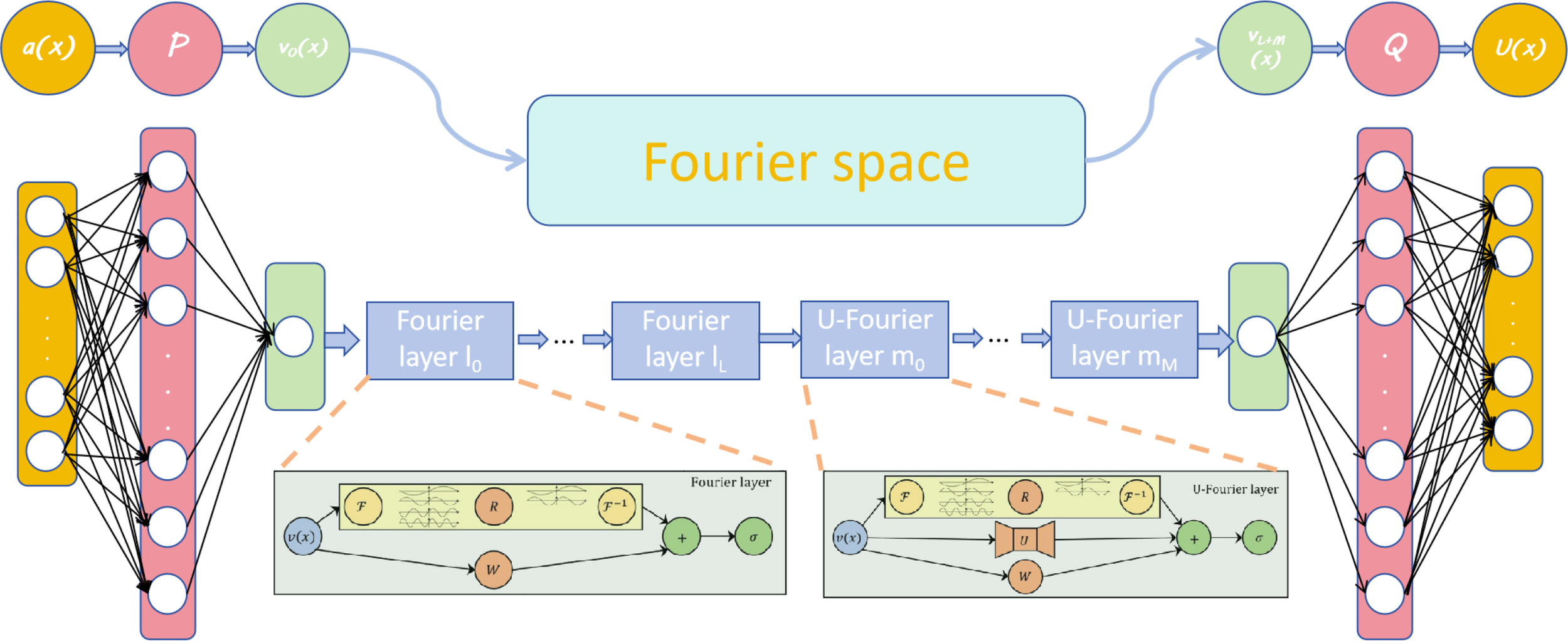
As shown in Figure 1a, the network input is first elevated to a higher dimension through a local transformation P (typically parameterized by a fully connected neural network):
Figure 1
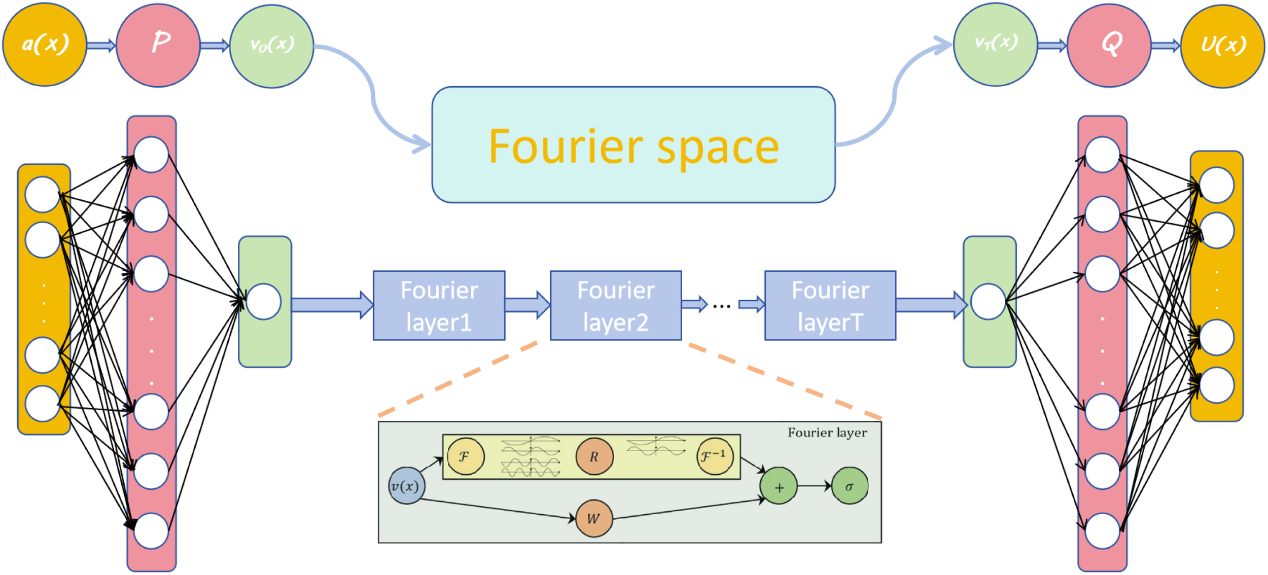
FNO network architecture diagram.
Then define each layer iteration update as:
The network output is
is the projection of Q achieved through local transformation .
Select as the kernel integral transformation parameterized by the neural network, defined as:
Where is a neural network parameterized by
The main idea behind FNOs is to choose a translation-invariant kernel function, which allows for efficient integration of the kernel using the fast Fourier transform (FFT) through convolution (Cooley and Tukey, 2023), multiplication in the feature space of fourier coefficients. is the Fourier transform and is the inverse Fourier transform. According to the Fourier convolution theorem, the integral function 2 is transformed into a Fourier space product form: .
Define the Fourier integral operator
where is the Fourier transform of a periodic function parameterized by .
constitutes the fundamental learnable component for extracting physical information from partial differential equations within Fourier space. The FNO methodology initiates by applying the Fourier transform to kernel functions, thereby replacing integration operations with spectrally efficient convolution. This transformation permits the representation of convolution as simple multiplication in Fourier coefficient space. To enhance generalization capacity and computational efficiency, high-order Fourier modes are truncated through a prescribed filtering strategy R, which retains the four dominant low-order modes.
In two-dimensional fourier transforms the primary energy concentration manifests within the four quadrants of the coefficient matrix—corresponding to low-frequency spectral regions. High-order modes, containing minimal energy contributions, predominantly encode structural details. The strategic elimination of these high-order modes consequently enhances model generalization performance and computational efficiency. The operational sequence culminates with an inverse Fourier transform to reconstruct spatial-domain representations. This spectral-spatial transformation demonstrates stronger congruence with physical governing equations than conventional convolution and recursive approaches (Tang and Fu, 2021; Li et al., 2021; Kovachki et al., 2023).
The time complexity of each layer of a CNN is , where N is the edge length of the feature graph, K is the edge length of the convolution kernel, Cin is the number of input channels and Cout is the number of output channels (Zhou et al., 2017; Dou et al., 2024). The time complexity of the FFT layer is , which is much faster than CNN.
2.2 Theory of parabolic equations in a two-dimensional cylindrical coordinate system
PEs are effective tools for simulating various phenomena in marine acoustics and can be used as effective numerical methods for range-related problems. Predicting pressure at one location based on complex pressure data at another location requires a model that accurately establishes the correlation between different spatial locations and environmental parameters.
When the time factor is exp(−iωt), the complex pressure function (r,z) and the frequency domain under the two-dimensional cylindrical coordinate P(r,z) satisfies the equation.
Where U(r,z) is the complex pressure after removing the forward column wave expansion term, then the complex pressure P(r,z) is expressed as
Where k0 is the reference wave number. In the far-field approximation k0r ≫ 1 it satisfies the equation:
Let the operators P and Q be
Equation 1 simplifies to the following:
The result after factorization is
Retaining the forward scattering term in the above equation, ignoring the backward scattering term, and ignoring the interaction term [P,Q], we obtain the general two-dimensional cylindrical coordinate acoustic field parabolic equation,
Where the operator be
The function satisfies the equations for
Starting from the initial field, in the weak distance-dependent case, for all range segments, let there be a pressure-releasing surface at z = zb. At each range segment the pressure field U(r,z) can be expressed as (Ivansson, 2017).
According to the Split-Step Padé (Collins, 1993) wide-angle parabolic equation algorithm, for r and r + Δr within the same range segment, the solution can be obtained analytically using the following equation:
We apply the Padé approximation,
We obtain the split-step Padé solution
2.3 Operator theory of sound field propagation
This study adapts the neural operator learning framework to the domain of underwater acoustic parabolic equation propagation. The deep architecture incorporates four cascaded Fourier integral operator layers, incorporating differential activation functions and batch normalization mechanisms.
Commencing from the initial acoustic field and invoking the weak range-dependence assumption, a pressure-release boundary condition is imposed at a depth of z = zbacross all range segments. In each range segment, the pressure field can be expressed as
kmis the modal wave number of the upper half-plane, corresponding to the corresponding modal function Zm and coefficients am.
According to Sturm-Liouville theory, the modal functions Zm from a complete set and are mutually orthogonal, with their norm defined as (Xu et al., 2023):
Where f is an analytic function in the space of square-integrable continuous functions on 0 ≤ z ≤ zb, with pressure-release boundaries at z = 0 and z = zb as well as the weight function ρ−1(z).
The space described by the above equation is the Banach space induced by this norm. It is not difficult to prove that, under this norm-induced metric, square-integrable functions form a complete metric space.
The proposed FNO-PE hybrid framework achieves integration with the traditional stepwise Padé algorithm through a three-stage collaborative process:
• Discrete field propagation. The computational domain employs a discrete grid with vertical resolution Δz = 1m, and range increment Δr = 10m. The sound speed profile c(z), density ρ(z), and spatial coordinates (r,z) are normalized to [-1, 1] per channel to mitigate feature scale divergence.
• Operator Learning Mechanism. The network input tensor integrates six physical fields: complex pressure amplitude components (ur,ui), wave number k, density ρ, and spatial coordinates r,z. The FNO architecture learns the mapping:
Replacing the conventional Padé expansion of . The Fourier layers explicitly resolve long-range dependencies through spectral convolutions, while local nonlinearities are captured via activated channel mixing.
• PML. A boundary treatment technique widely used in numerical acoustics to absorb incident acoustic waves at the computational domain boundary, eliminating spurious reflections that would interfere with the internal sound field simulation and ensuring accurate boundary conditions (Jensen, 2011).Here, PML is implemented through complex coordinate stretching beneath the seafloor interface zb(r). The absorption coefficient γ(z) is parameterized as:
This adaptive impedance matching minimizes spurious reflections while preserving trainset compatibility.
The framework expands channel dimensionality to accommodate multiparameter acoustic representations, with its input-output structure explicitly defined as follows: Input xi:A single input sample, forming an overall fourth-order input tensor . Here, N is the number of training samples, κ × κ is the wavenumber-space grid size (ensuring spatial discretization consistency), and the 6 channels correspond to 6 core physical fields: complex pressure amplitude(real part ur, imaginary part ui), wave number k, seawater density ρ, radial coordinate r, and vertical coodinate z. Each channel is normalized to [−1,1] to eliminate feature scale bias, with raw data derived from the RAM v1.5 platform.
Output yi: A single output sample, forming an overall fourth-order output tensor . Here, N matches the input sample count, κ × κ is consistent with the input wavenumber grid (spatial alignment), and Ty denotes the number of temporal evolution steps———i.e., the model predicts the complex sound pressure field at Ty consecutive radial ranges (e.g., to ). The reference values of yi are also obtained from RAM v1.5, serving as the target for model training.
This approach demonstrates enhanced numerical stability over traditional PE methods through continuous operator learning, enabling large-scale scalable simulations of acoustic propagation over complex bathymetric features.
2.4 Origin of time complexity
The computational efficiency of the proposed FNO-PE framework stems from its grid-independent spectral convolution architecture. To clarify the superiority of this design over the conventional RAM method (split-step Padé parabolic equation solver), the time complexity of both methods and the core advantage of FNO—grid invariance—are systematically elaborated below.
The FNO module in the hybrid framework achieves O(nlogn) time complexity, which originates from its spectral convolution mechanism. FNO approximates the acoustic propagation operator by converting the input complex pressure field U(r, z) between the spatial and wavenumber domains using Fast Fourier Transform (FFT) and Inverse FFT (IFFT)—operations with mathematically proven O(n log n) complexity.
After FFT, FNO retains only low-frequency Fourier modes (kmax = 12 in this study) to capture dominant physical features (e.g., modal interference in shallow-water acoustics), while the complexity of mode truncation and subsequent linear transformation (via the weight tensor R) is , where dvis the fixed feature channel dimension). Since kmax ≪ n and dvdoes not scale with grid size, this overhead is negligible, leaving FFT/IFFT as the dominant contributor to the scaling.
The traditional RAM method exhibits theoretical linear time complexity (O(n), derived from its split-step Padé core. RAM decomposes acoustic propagation into discrete range steps, and at each step, it solves tridiagonal linear systems using the Thomas algorithm—a specialized Gaussian elimination method that leverages matrix sparsity to achieve (O(n) complexity per step. The number of range steps in RAM is determined by the total propagation distance and fixed adaptive step size, resulting in a constant number of steps independent of n; thus, the overall complexity scales linearly with n.
While RAM achieves theoretical (O(n) complexity, its practical efficiency is severely constrained by grid dependence—a limitation that FNO overcomes via inherent grid invariance. This property is the key to FNO’s superiority in underwater acoustic applications.
RAM is a grid-bound numerical method. For any change in spatial resolution, RAM requires full reinitialization of the computational mesh, adjustment of the split-step Padé step size, and re-solving of tridiagonal systems from scratch—introducing “resolution-switching overhead” that is not reflected in its theoretical (O(n) complexity. Furthermore, for complex marine environments, RAM demands manual grid refinement, which increases the effective n and elevates practical computational costs far beyond the theoretical linear scaling.
FNO’s grid invariance originates from its spectral-domain parameter learning: the Fourier modes kmax and weight tensor R (learned in the wavenumber domain) are resolution-independent—they remain unchanged regardless of grid size. Consequently, the FNO-PE framework requires only one-time training and can be directly applied to other resolutions without retraining or parameter tuning. For complex scenarios, FNO maintains stable scaling and inference time, avoiding the additional overhead of RAM’s grid refinement.
2.5 Data description
This chapter outlines the data generation methodology using the MATLAB-based RAM v1.5 acoustic modeling platform, which involves constructing both training and multi-condition test datasets. The primary objective involves rigorously validating the FNO framework’s robustness and computational efficiency across diverse marine environmental parameters.
For the 2D underwater acoustic computational domain (radial distance r × vertical depth z), n is uniformly defined as the total number of spatial grid points(i.e., n = Nr × Nz, where Nr and Nz denote the number of grid points along the range and depth dimensions, respectively). This definition aligns with the foundational FNO theory (Li et al., 2021) and ensures consistent complexity comparison.
2.5.1 Data preparation
The Pekeris waveguide configuration comprises a uniform seawater layer (z1 = 200m, c1 = 1500m/s, ρ = 1.0g/cm3) overlying a semi-infinite sediment layer (c2 = 1600m/s, ρ = 1.8g/cm3). The computational domain spans (r0,z0) = (0,0) to (rmax, zmax) = (10km, 400m) with sediment absorption neglected. A perfectly matched layer (PML) boundary condition terminates the domain at z = 400m, as illustrated in Figure 2.
Figure 2
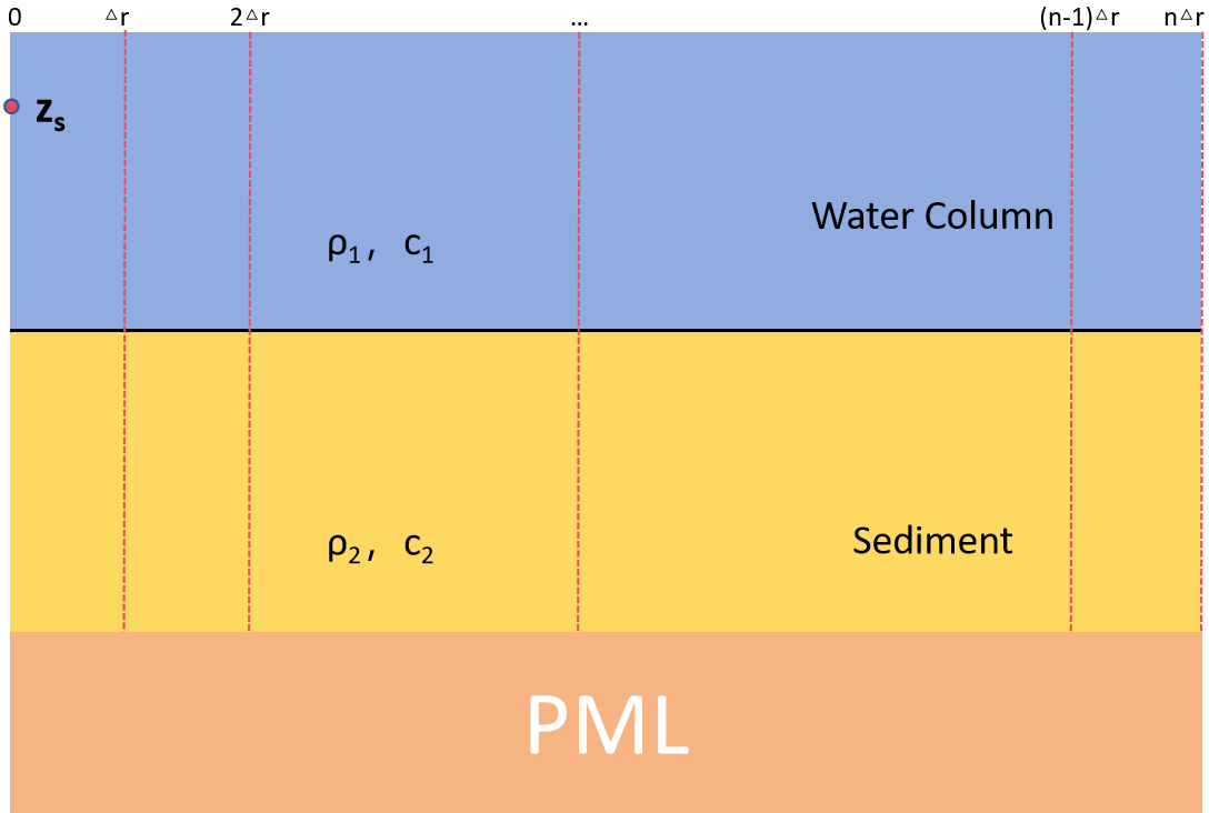
Computational domain.
The verification framework systematically examines two critical dimensions: sound source variability and environmental heterogeneity. For source parameter analysis, six frequencies (40–100 Hz) at 50 m depth assess frequency response characteristics spanning 40% to 160% of standard shallow-water sonar frequencies (50 Hz reference). Vertical adaptability is evaluated through six source depths (10–100 m) using a 50 Hz reference, with specific emphasis on near-surface (< 30m depth) and shallow-water (< 200m depth) configurations. This methodology reveals the depth-dependent effects of sound field distribution on model generalization.
Environmental variability testing incorporates three critical elements: (1) Sound velocity profile effects assessed through uniform, positive-gradient, and negative-gradient structures; (2) Seabed terrain impacts evaluated via 5°− 15° slope geometries simulating reflection path distortions; (3) Deep-sea adaptability validated through domain extension to 4000 m depth (2000 m seawater and 2000 m sediment) with preserved PML conditions. This multivariate test matrix—spanning source parameters, medium properties, and geometric boundaries—establishes a rigorous evaluation benchmark, ranging from shallow to deep marine environments, enabling a quantitative assessment of model robustness, accuracy, and computational efficiency.
2.5.2 Model evaluation
Model performance is quantified through two primary metrics: the relative root mean square error (RMSE error) and the coefficient of determination (R2 Score). These measure divergence between FNO predictions and RAM-generated reference solutions, with R2 → 1 indicating optimal regression fidelity.
Where n is the number of spatial grid points in the water column; denotes the FNO-predicted complex pressure (real/imaginary part) at grid point i; yi denotes the RAM-generated reference pressure (real/imaginary part) at the same grid point; is the L2-norm, and the result is converted to decibel (dB) units to align with acoustic field measurement conventions.
Where is the mean value of the RAM reference pressure over the spatial grid. An indicates the FNO prediction fully captures the variability of the true acoustic field.
2.5.3 Performance comparison protocol
Performance is compared against the conventional RAM method (the gold standard for parabolic equation based acoustic simulation) across all validation scenarios, with two core comparison dimensions: accuracy comparison and efficiency comparison.
For each scenario, compute R2(real/imaginary parts) and RMSE (dB) of the FNO and RAM solutions. To mitigate randomness from network initialization, statistical significance is ensured by averaging metrics over 3 independent runs. Measure the average inference time of FNO and RAM under the same hardware. For large-scale scenarios, record the absolute computation time and relative acceleration ratio to quantify efficiency gains.
2.6 Benchmark model validation
2.6.1 Network construction and hyperparameter optimization
Based on the rigorous optimization of pre-training and systematic ablation experiments, this work employs the following hyperparameter configuration to construct a Fourier neural operator architecture. The model features a six-layer structure comprising an input/output linear transformation layer and a four-layer Fourier spectral convolution. The weight matrix is initialized by a proportional hyperbolic tangent function with parameter θ = 1.0001 to maintain gradient stability. The original high-resolution ocean sound field data is input into the network using a 2:1 downsampling strategy to achieve an effective balance between sound field detail retention and memory consumption. In the optimization process, the first-order moment estimation β1 = 0.9 and the second-order moment estimation β2 = 0.999 of the fixed Adam algorithm are fixed to ensure the mathematical completeness of the bias correction in the gradient update process.
The FNO’s function space mapping operates on Banach subspaces bounded by waveguide interfaces, with sub-bottom data treated as environmental noise. Consequently, all visualizations in this section exclusively depict water column sound field distributions, excluding interactions with the seabed.
2.6.2 Model performance evaluation under different nonlinear transfer mechanisms
Activation functions are a critical component in neural networks, applied to individual neurons to introduce non-linearity into the input signals before propagating the transformed outputs to subsequent layers. In neural network training, several commonly used activation functions stand out, including the hyperbolic tangent function (Tanh(x)), rectified linear unit (ReLU(x)), sigmoid function (Sigmoid(x)), and leaky rectified linear unit (Leaky ReLU(x)). Visualizations of these four functions are provided in Figure 3. Under controlled Pekeris waveguide conditions (f=50 Hz, z=50 m), ReLU achieved superior complex pressure reconstruction (R2Re = 0.9662, R2Im = 0.9676) compared to Tanh (△R2 = ±9.56%) and Leaky ReLU (△R2 = ±8.73%). As shown in Figure 4, the result indicates ReLU’s advantage for parabolic equation solvers requiring long-range waveform fidelity.
Figure 3
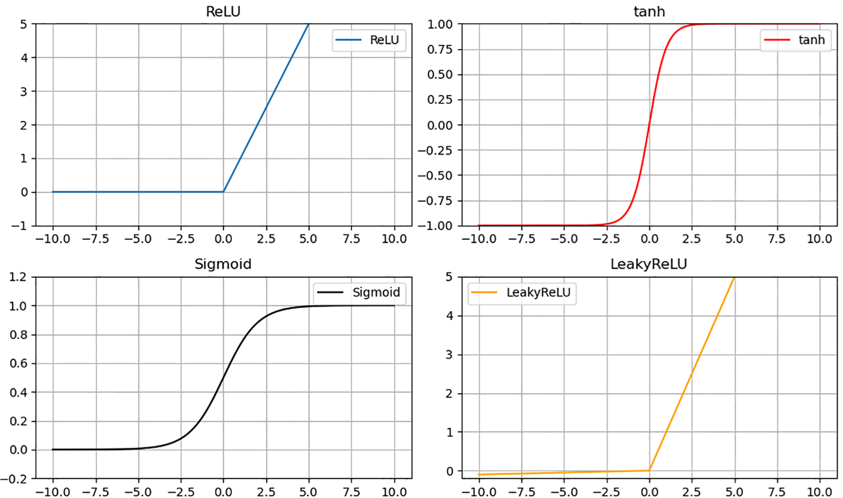
Activation functions.
Figure 4
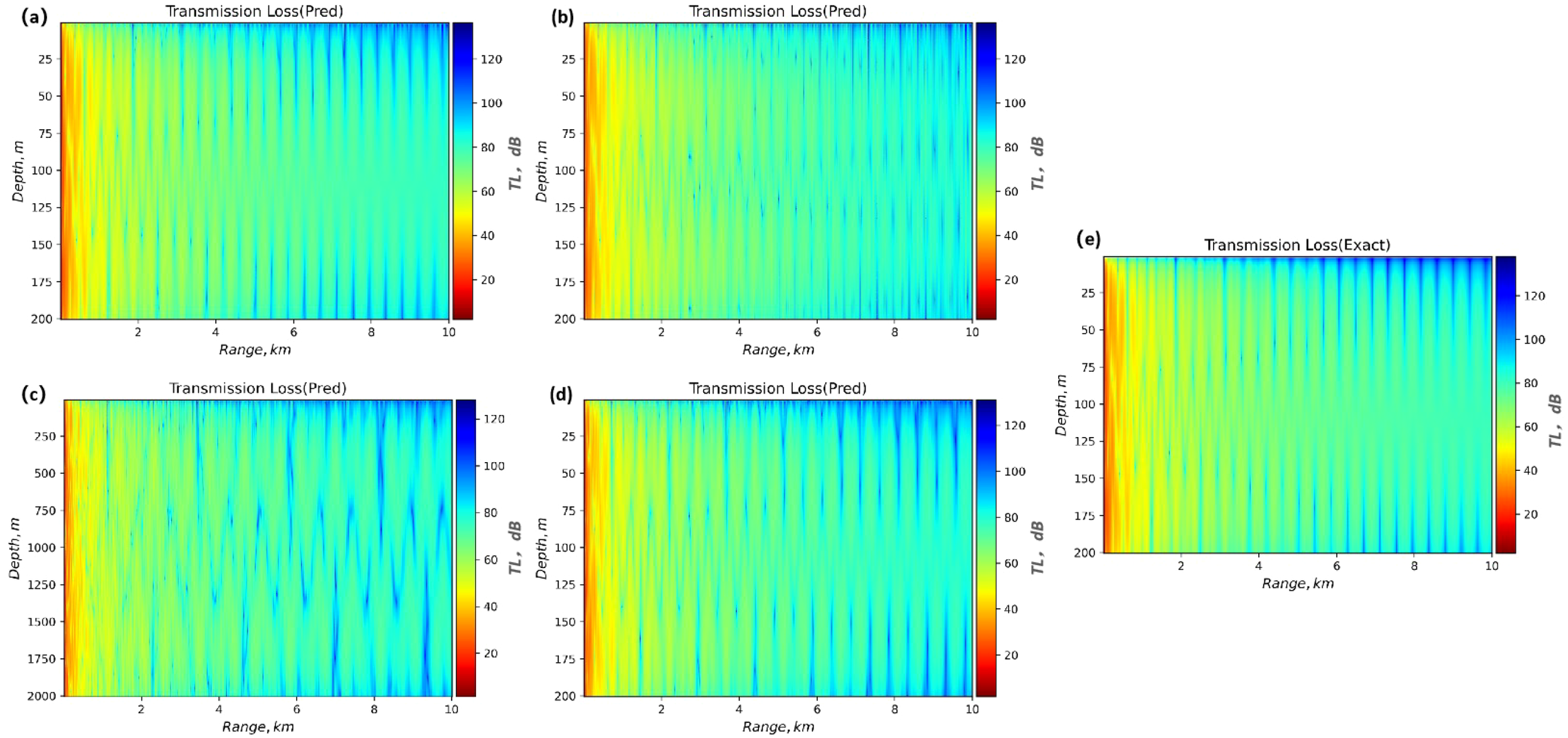
Comparison of predicted transmission loss by different activation functions with RAM results. (A) ReLU-Predicted Transmission Loss. (B) Tanh-Predicted Transmission Loss. (C) SigmoidPredicted Transmission Loss. (D) Leaky ReLU-Predicted Transmission Loss. (E) RAM-Exact Transmission Loss.
3 Results and discussion
3.1 Robustness verification experiment of sound source disturbance
3.1.1 Performance evaluation of different sound source frequency
The frequency generalization capability was rigorously tested using a model trained at 40 Hz and evaluated across five discrete frequencies (50, 60, 70, 80 and 100 Hz). To quantify the frequency-dependent energy attenuation of acoustic waves in seawater, we introduced the seawater acoustic absorption coefficient alpha(f) (dB/km)). This coefficient integrates three dominant attenuation mechanisms in seawater and follows the classical Thorp absorption model (Jensen, 2011).
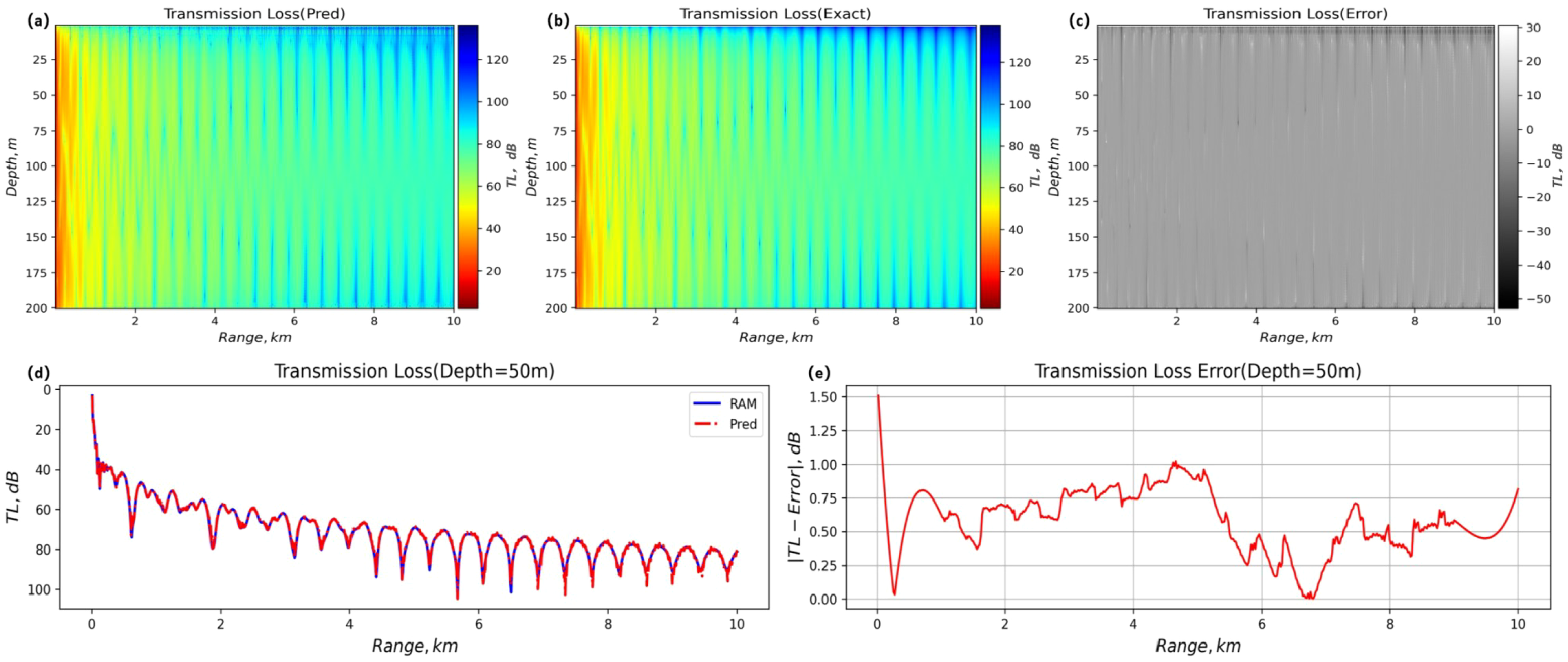
The evaluation results of the model’s frequency generalization ability show that the model exhibits stable generalization in the frequency range of 50–100 Hz. As shown in Appendix Table A3 in Supplementary Material, the prediction accuracy decays gradually with the increase of frequency, but the model always maintains RMSE < 0.042dB through the core features captured by the Fourier space convolution kernel. It is found that there is approximately 2.8 − 3.1% R2 attenuation in every 10 Hz band, which is closely related to the high-order Fourier mode stage. FNO completes the prediction in 2.89 ± 0.16s, which is 25% − 35% faster than RAM. This study demonstrates that the framework can offer technical support for the trial sound field prediction of broadband sonar systems and can be applied to multi-source detection scenarios in complex marine environments. Figure 5 shows the propagation loss at the test frequency of 50 Hz.
Figure 5
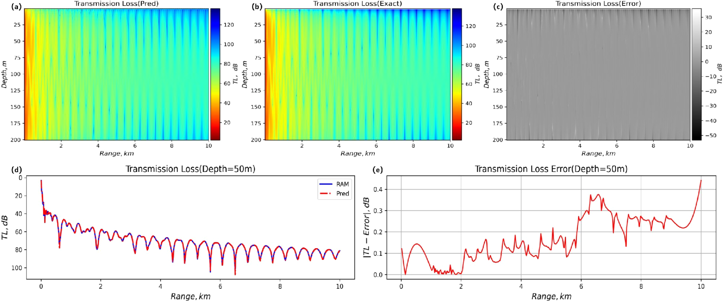
Comparison of sound transmission loss, error diagrams, and two-dimensional curves between FNO and RAM at a test frequency of 50 Hz. (A) Predicted transmission loss. (B) Exact transmission loss. (C) Transmission loss error. (D) Two-dimensional propagation loss curve. (E) Transmission error plot.
3.1.2 Performance evaluation of different sound source positions
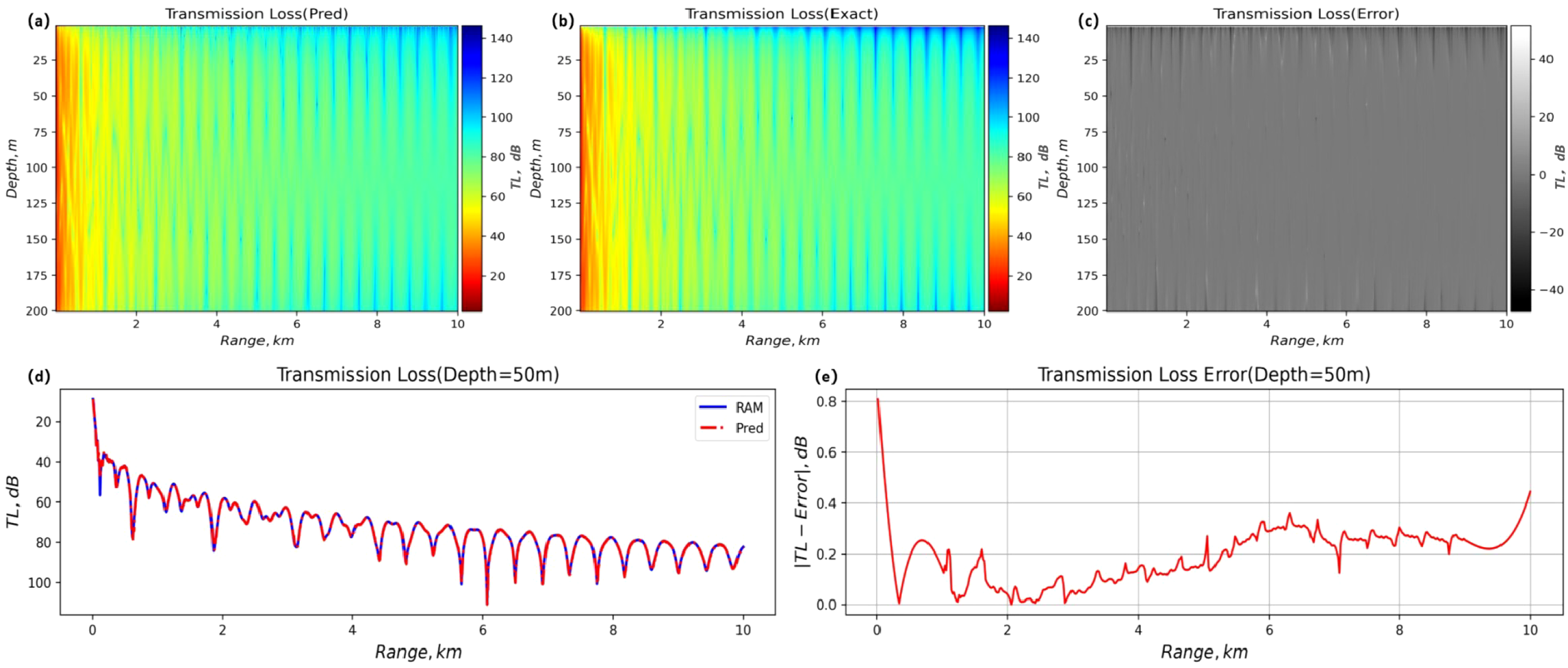
This section is based on the zs= 60m sound source (f = 50Hz) training model, and the generalization performance test is carried out in the depth range of [10, 30, 40, 50, 100 m] sound sources. As shown in Appendix Table A4 in Supplementary Material, the framework exhibits strong generalization robustness to the vertical localization of sound sources, with a determination coefficient (R2) of the complex sound pressure component exceeding 0.89 under all verification conditions. The optimal prediction performance is obtained at a depth of zs= 50m: the real part R2 = 0.9462, the imaginary part R2 = 0.9476, and the corresponding root mean square error , , which is significantly better than the shallow and deep sound source configuration. Figure 6 is the propagation loss at a test source position of 50 m. When the sound source depth is z = 10 m and the receiving depth is 50 m, the error converges to approximately 0.3 dB within 1 km of propagation, and the calculation time remains stable at 2.81 ± 0.16s, which is 25.3% lower than the RAM reference method. The indiscriminate acceleration characteristics of sound source depth verify the technical adaptability of this operator method in the application of a vertical receiving array.
Figure 6
Comparison of sound transmission loss, error diagrams, and two-dimensional curves between FNO and RAM at a test source position of 50 m. (A) Predicted transmission loss. (B) Exact transmission loss. (C) Transmission loss error. (D) Two-dimensional propagation loss curve. (E) Transmission error plot.
3.2 Generalization ability assessment of non-uniform marine environment
3.2.1 Performance evaluation of different sound velocity profiles
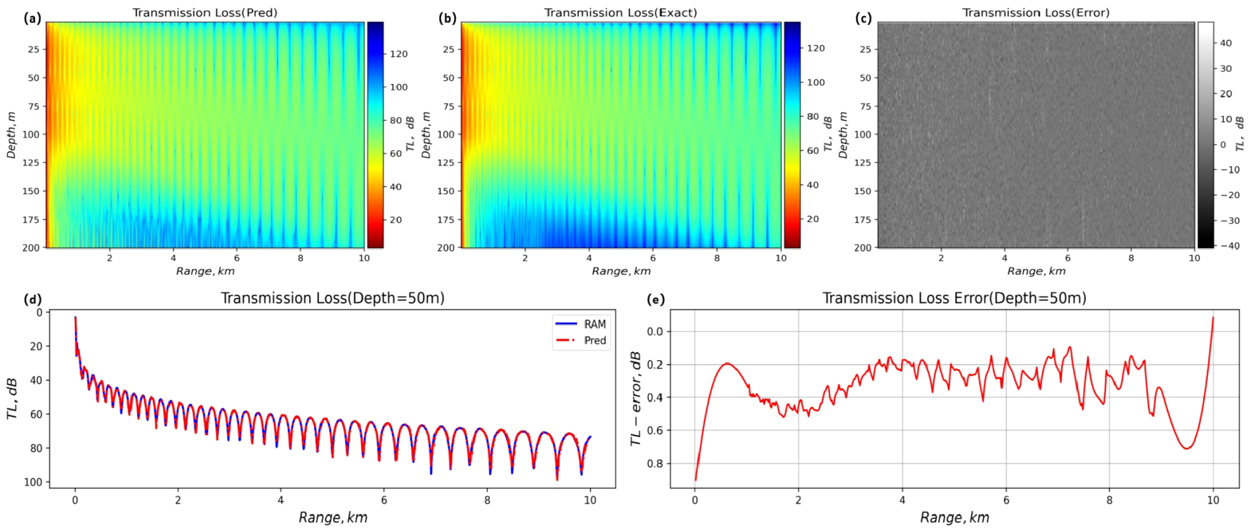
As the core influencing factor of underwater acoustic propagation law, the spatial heterogeneity of the sound velocity profile is the key consideration for constructing a sound field prediction model. In this study, the FNO network trained under uniform sound velocity conditions is utilized for transfer learning verification in two typical non-uniform sound velocity fields: positive gradient and negative gradient. The experimental data are generated based on the sound source with zs= 40 m and f = 50 Hz. Figure 7 clearly shows the two-dimensional distribution and propagation curve characteristics of sound field propagation loss under uniform sound velocity.
Figure 7
Comparison of sound transmission loss, error diagrams, and two-dimensional curves between FNO and RAM under uniform sound velocity profiles. (A) Predicted transmission loss. (B) Exact transmission loss. (C) Transmission loss error. (D) Two-dimensional propagation loss curve. (E) Transmission error plot.
The numerical results show that the model’s prediction accuracy, as measured by the RMSE, is less than 0.016 dB in the uniform sound velocity scene, which verifies the effective analysis of the steady-state waveguide multimode interference characteristics using the Fourier convolution kernel. However, the non-uniform sound velocity condition significantly increases the training complexity. The negative gradient sound velocity field requires 2400 iterations to converge, which is three times more training time than the uniform scene, and the verification loss value increases by two orders of magnitude. The positive gradient sound velocity field yields a negative value of the determination coefficient (R2< 0), indicating that the model’s prediction result is inferior to the uniform sound velocity condition and significantly differs from the exact value. This phenomenon arises from the inherent limitations of the isotropic Fourier convolution kernel under refraction conditions: it is challenging to analyze the direction-dependent acoustic scattering path, leading to the failure of spectral space parametric mapping. This finding reveals the sensitivity of the existing architecture to the strong vertical sound velocity gradient. In the next step, the empirical orthogonal function (EOF) expansion of the finite term will be used to approximate the changing sound velocity profile, thereby improving the modeling ability of the non-uniform sound field.
3.2.2 Performance evaluation of different slope terrain
To evaluate the influence mechanism of slope topography on sound field propagation, this study constructs a slope seabed model to simulate the propagation process of acoustic oblique incidence. Figure 8 shows the distribution and curve of two-dimensional propagation loss under this condition. The experimental results show that, with the fluctuation of seabed terrain slope, the sound propagation loss value predicted by the model exhibits obvious terrain-dependent characteristics, and its cumulative attenuation rate is 12.7 ± 3.5dB/km higher than that of flat seabed conditions. The propagation loss curve shows a significant time-domain interference fringe enhancement phenomenon in the depth-distance domain space. This phenomenon can be attributed to the multi-modal coupling effect caused by the increase in the number of bottom-contact reflections (shortened bottom-contact period) at the wave level. The physical mechanism is that the acoustic phase delay caused by the sudden change of terrain is , which leads to the multipath effect.
Figure 8
Comparison of sound transmission loss, error diagrams, and two-dimensional curves between FNO and RAM at a slope angle of 15°. (A) Predicted transmission loss. (B) Exact transmission loss. (C) Transmission loss error. (D) Two-dimensional propagation loss curve. (E) Transmission error plot.
3.2.3 Performance evaluation of deep-sea region
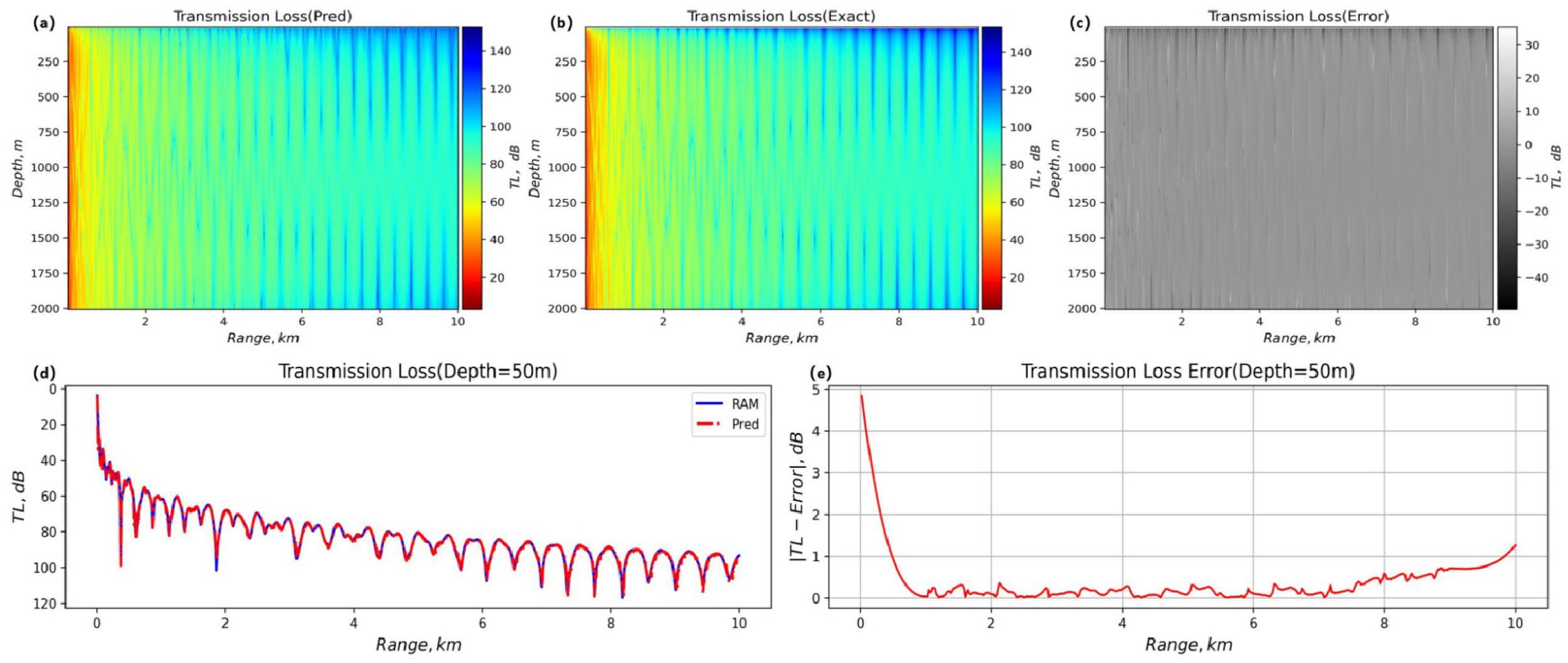
This study extends the computational domain to 4000 meters of deep-sea space for systematic verification, aiming to assess the model’s generalization performance in the complex deep-sea environment. Based on the FNO network trained by the sound source with zs= 200 m and f = 50 Hz, the sound field prediction of the extended domain under the conditions of zs = 500 m and zs = 100 m is successfully realized (Figure 9).
Figure 9
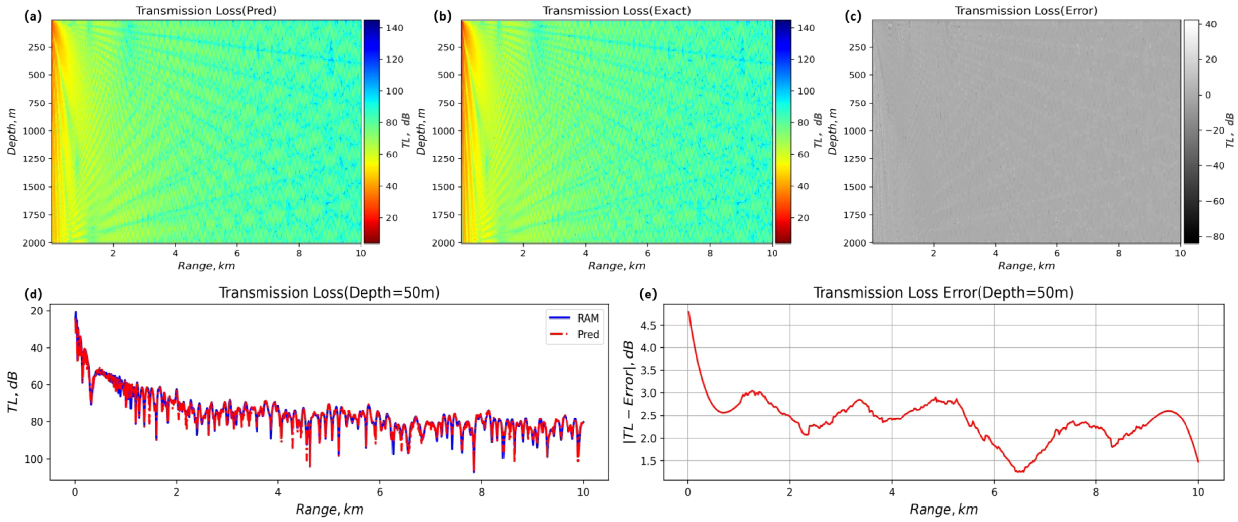
Comparison of sound transmission loss, error diagrams, and two-dimensional curves between FNO and RAM under deep-sea conditions. (A) Predicted transmission loss. (B) Exact transmission loss. (C) Transmission loss error. (D) Two-dimensional propagation loss curve. (E) Transmission error plot.
The numerical verification data show that (Appendix Table A7 in Supplementary Material): In the sound field range of 100 m sound source depth, the average determination coefficients of the complex sound compaction part and the imaginary part reach R2Re = 0.9058 and R2Im = 0.8879, respectively, and the relative root mean square error is stable at = 0.0408 dB and = 0.0456 dB. The two-dimensional loss distribution of sound field propagation and the two-dimensional propagation loss curve further reveal that the error distribution of the model in the deep-sea water area is uniform (Figure 9). This feature is due to the efficient feature extraction ability of the FNO spectral convolution kernel, which effectively captures the low-frequency modal interference and energy diffusion effects in deep-sea channels through an adaptive frequency-domain filtering mechanism. The experimental results demonstrate that the framework achieves sub-decibel-level sound field reconstruction in the kilometer-level depth domain, providing an efficient computing paradigm for deep-sea cross-scale acoustic modeling, such as predicting deep-sea channel convergence zones and inverting seabed acoustic parameters.
3.3 Computational efficiency analysis
The chart system of numerical calculation efficiency analysis reveals the computational superiority of FNO in five types of marine acoustic scenarios. Taking the trend analysis presented in Figure 10 as an example, compared with the traditional RAM method, the proposed method achieves an average delay reduction of 28.4 ± 6.7%, and the acceleration effect reaches a peak of 38.7% under typical uniform sound speed profile conditions, even in complex deep-sea environments. It still maintains a baseline acceleration ratio of 25.3%. This phenomenon verifies the spectral convolution operator’s theoretical characteristics from the engineering practice perspective: through the time complexity of O(nlogn), the computational efficiency is significantly better than the time complexity strategy of the traditional finite difference method.
Figure 10
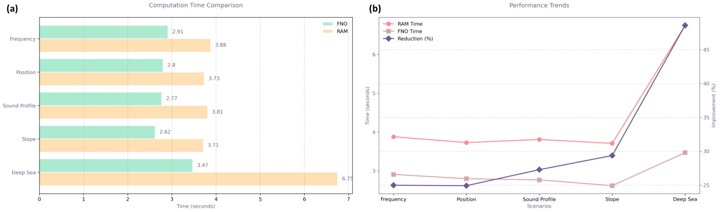
Computation time comparison. (A) Average duration of FNO and RAM under different experimental conditions. (B) Changes in the average duration of FNO and RAM under different experimental conditions and improvement efficiency.
The time series evolution characteristics further reveal the stable acceleration mechanism of the algorithm: the model achieves a 32.8% delay reduction under the benchmark condition (the calculation time is 2.77 seconds vs. 3.68 seconds) in the face of environmental perturbations such as sound source frequency/position changes, it can still maintain a robust performance of 29.1 ± 1.2%. In particular, it is worth noting that the model continues to demonstrate a stable acceleration capability of 27.5% for complex hydrodynamic scenarios with sloping terrain and deep-sea cross-scale conditions. When extended to deep-sea conditions with a water depth of 4000 meters, the FNO deduction time is strictly controlled within 3.5 seconds. Compared with the 6.75 seconds of the RAM method, the absolute acceleration ratio is 2.95 times. The improvement can be attributed to the theoretical avoidance of the iterative solution process of the Helmholtz equation by the Fourier space projection mechanism in the framework, and the model’s low sensitivity to sound source parameters is mathematically verified at the L2(D) solution space continuity level.
The empirical results are in strict agreement with the theoretical expectations of Section 2.3: the invariance of spatial discretization ensures the stability advantage of the algorithm in the variable grid system, which is particularly important in the three-dimensional extended scene.
Although RAM exhibits theoretical linear complexity, its grid dependence makes it inefficient in practical underwater acoustic prediction—especially for multi-resolution tasks (e.g., shallow-to-deep sea extrapolation) and complex environments. In contrast, FNO’s complexity, when combined with grid invariance, delivers three critical advantages: (1) eliminating resolution-switching costs; (2) avoiding manual grid tuning for heterogeneous scenarios; (3) enabling rapid generalization across a family of acoustic propagation problems (e.g., 40–100 Hz broadband sources). As validated in Section 3.2.3, even for 4000 m deep-sea simulation, FNO’s inference time remains < 3.5s—25%–35% faster than RAM—while maintaining sub-decibel accuracy (RMSE < 0.045,dB). This confirms that the FNO-PE framework is a more efficient and robust solution for large-scale underwater acoustic field prediction than the traditional RAM method.
3.4 Multi-scale sound field fusion enhancement mechanism of U-FNO architecture
The enhanced U-FNO architecture addresses spectral regularization limitations by integrating U-Net modules after Fourier layers in the baseline FNO framework (Wen, 2022).
While standard FNO demonstrates exceptional test accuracy, its spectral regularization effects hinder training convergence. To resolve this, we propose the U-Fourier layer with the mathematical formulation:
Where denotes the kernel integral transform in Fourier space, represents the U-Net convolutional path for local refinement, and W corresponds to linear projection. This hierarchical design enables Fourier transforms to capture global wavefield patterns while subsequent U-Net modules resolve boundary-induced local distortions.
The network architecture is shown in Figure 11 by extending the network channel dimension to be compatible with six-dimensional input features: sound pressure complex amplitude component (ur, ui), wave number k, density ρ, and spatial coordinates (r, z), and configuring four layers of U-Fourier layer with spectral mode truncation strategy.
Figure 11
U-FNO network architecture diagram.
Experimental results demonstrate U-FNO’s superior accuracy over standard FNO across marine environments. In shallow-water scenarios with a 60 Hz source, the hybrid architecture achieves R2Re = 0.9850 and R2Im = 0.9842, with RMSE stabilized at R2Re = 0.0103 dB and R2Im = 0.0119 dB. For 4,000m deep-sea conditions (consistent with Section 3.2.3), it maintains R2Re = 0.9824 and R2Im = 0.9833 in upper layers and full-depth predictions—significantly outperforming the baseline FNO. The two-dimensional propagation loss distribution and axial attenuation curves under these conditions are detailed in Figure 12 respectively, highlighting U-FNO’s efficacy in suppressing seabed multipath artifacts.
Figure 12
Comparison of sound transmission loss, error diagrams, and two-dimensional curves between FNO and RAM. (A) Predicted transmission loss. (B) Exact transmission loss. (C) Transmission loss error. (D) Two-dimensional propagation loss curve. (E) Transmission error plot.
4 Conclusion and summary
This study establishes an FNO-enhanced framework for solving underwater acoustic parabolic equations, effectively resolving the accuracy-efficiency trade-off inherent in conventional Split-Step Padé methods. The proposed approach achieves grid-independent solutions by integrating spectral convolution with acoustic propagation physics while maintaining rigorous physical consistency. The framework introduces a multi-channel input mechanism incorporating the acoustic field U(r,z), wavenumber k, and density ρ, replacing iterative Padé expansions with Fourier domain projections. This design exploits FNO’s spectral invariance to establish global sound field correlations through wavenumber-domain mode truncation mechanisms, demonstrating a coefficient of determination exceeding 0.95 across multipath-dominant shallow water and deep-sea environments.
The spectral convolution scheme reduces computational latency by 25%–35% compared to conventional RAM methods, consistently maintaining inference times below 3.5 seconds in kilometer-scale deep-sea simulations. In complex marine environments, the framework demonstrates robust adaptability to slope bathymetry (5–15°), exhibiting propagation loss attenuation rates elevated by 12.7 ± 3.5dB/km relative to planar bathymetries, with post-reflection cumulative errors converging below 0.3 dB. When extended to 4,000-m deep-sea conditions, it maintains sub-decibel reconstruction accuracy (RMSE < 0.045dB) for complex pressure fields. These results confirm the FNO’s capability to resolve low-frequency modal interference and energy diffusion phenomena.
However, performance degradation occurs under non-uniform sound speed gradient profiles, where isotropic convolutional kernels fail to capture refraction-induced acoustic paths, yielding negative R2 coefficients. Regarding the model’s prediction failure under non-uniform sound speed gradient profiles, the decomposition of sound speed profiles based on EOF can serve as a core improvement direction. EOF is capable of decomposing complex and inhomogeneous positive-gradient sound speed fields into a small number of principal modes that dominate energy (typically the first 3–5 orders can explain over 90% of sound speed variation), effectively stripping redundant information and highlighting the key structure of gradient directions. This characteristic has been widely applied in underwater acoustics for the characterization of sound speed in stratified media such as surface ducts and thermoclines. For instance, in shallow-water positive-gradient scenarios, the first two EOF orders can respectively describe the average sound speed baseline and gradient change rate, accurately capturing the directional dependence of sound ray refraction.
The specific technical pathway can be designed as follows: the principal mode parameters (modal coefficients, eigenvalues) obtained from EOF decomposition are used as supplementary input features for the FNO, replacing the original sound speed profile data. Combined with an adaptive spectral mode truncation strategy, the Fourier convolution kernel can focus on the refraction path information corresponding to the EOF principal modes, overcoming the limitation that the current isotropic kernel cannot resolve direction-dependent scattering.
These advancements will establish next-generation intelligent ocean acoustic computation frameworks, providing critical theoretical foundations for deep-sea exploration systems. Subsequent research will develop hybrid FNO-FEM solvers using the South China Sea experimental datasets, targeting balanced performance metrics: acoustic reconstruction accuracy (RMSE< 0.02dB) and computational efficiency (35% acceleration relative to conventional finite element methods under complex boundary conditions).
Statements
Data availability statement
The raw data supporting the conclusions of this article will be made available by the authors, without undue reservation.
Author contributions
XZ: Investigation, Writing – original draft, Writing – review & editing, Formal analysis, Methodology, Conceptualization, Data curation. HX: Supervision, Writing – review & editing. HW: Software, Supervision, Writing – original draft, Visualization, Validation. CZ: Data curation, Visualization, Writing – review & editing. JD: Investigation, Validation, Writing – review & editing. JL: Project administration, Writing – review & editing, Funding acquisition, Resources. ST: Validation, Supervision, Conceptualization, Writing – original draft.
Funding
The author(s) declared that financial support was received for this work and/or its publication. This work was supported by the National Natural Science Foundation of China (52501427), the National Basic Research Program of China (50916060703, 2024-JCJQ-QT-006).
Acknowledgments
The authors would like to acknowledge the use of the FNO model.
Conflict of interest
The authors declared that this work was conducted in the absence of any commercial or financial relationships that could be construed as a potential conflict of interest.
Generative AI statement
The author(s) declared that generative AI was not used in the creation of this manuscript.
Any alternative text (alt text) provided alongside figures in this article has been generated by Frontiers with the support of artificial intelligence and reasonable efforts have been made to ensure accuracy, including review by the authors wherever possible. If you identify any issues, please contact us.
Publisher’s note
All claims expressed in this article are solely those of the authors and do not necessarily represent those of their affiliated organizations, or those of the publisher, the editors and the reviewers. Any product that may be evaluated in this article, or claim that may be made by its manufacturer, is not guaranteed or endorsed by the publisher.
Supplementary material
The Supplementary Material for this article can be found online at: https://www.frontiersin.org/articles/10.3389/fmars.2025.1692899/full#supplementary-material
References
1
Berg J. Nyström K. (2018). A unified deep artificial neural network approach to partial differential equations in complex geometries. Neurocomputing317, 28–41. doi: 10.1016/j.neucom.2018.06.056
2
Collins M. D. (1993). A split-step padé solution for the parabolic equation method. J. Acoustical Soc. America93, 1736–1742. doi: 10.1121/1.406739
3
Collins M. D. (2012). A single-scattering correction for the seismo-acoustic parabolic equation. J. Acoustical Soc. America131, 2638–2642. doi: 10.1121/1.3689557
4
Collins M. D. Dacol D. K. (2000). A mapping approach for handling sloping interfaces. J. Acoustical Soc. America107, 1937–1942. doi: 10.1121/1.428476
5
Cooley J. W. Tukey J. W. (2023). An algorithm for the machine calculation of complex fourier series. Mathematics Comput.
6
Dissanayake M. W. M. G. Phan-Thien N. (1994). Neural-network-based approximations for solving partial differential equations. Commun. Numerical Methods Eng.10, 195–201. doi: 10.1002/cnm.1640100303
7
Dou H. Zhang L. Han F. Shen F. Zhao J. (2024). Review of studies on interpretability of convolutional neural networks. J. Software35, 159–184. doi: 10.13328/j.cnki.jos.006758
8
Du L. Wang Z. Lv Z. Wang L. Han D. (2023). Research on underwater acoustic field prediction method based on physics-informed neural network. Front. Mar. Sci.10. doi: 10.3389/fmars.2023.1302077
9
Hinze M. Pinnau R. Ulbrich M. Ulbrich S. (2009). Optimization with PDE Constraints Vol. 23 Mathematical Modelling: Theory and Applications (Dordrecht: Springer Netherlands). doi: 10.1007/978-1-4020-8839-1
10
Hornik K. Stinchcombe M. White H. (1989). Multilayer feedforward networks are universal approximators. Neural Networks2, 359–366. doi: 10.1016/0893-6080(89)90020-8
11
Ivansson S. (2017). “ Chapter 3 - sound propagation modeling,” in Applied Underwater Acoustics. Eds. NeighborsT. H.BradleyD. (Amsterdam, Netherlands: Elsevier), 185–272. doi: 10.1016/B978-0-12-811240-3.00003-5
12
Jensen F. B. (2011). Computational Ocean Acoustics. Modern Acoustics and Signal Processing. 2nd ed (New York: Springer).
13
Kovachki N. Li Z. Liu B. Azizzadenesheli K. Bhattacharya K. Stuart A. et al . (2023). Neural operator: learning maps between function spaces. arXiv preprint arXiv:2108.08481.
14
Lagaris I. Likas A. Fotiadis D. (1998). Artificial neural networks for solving ordinary and partial differential equations. IEEE Trans. Neural Networks9, 987–1000. doi: 10.1109/72.712178
15
Lake L. Johns R. T. Rossen W. R. Pope G. A. (2024). Fundamentals of Enhanced Oil Recovery (Richardson, TX, USA: Society of Petroleum Engineers). doi: 10.2118/9781613993286
16
Li Z. Kovachki N. Azizzadenesheli K. Liu B. Bhattacharya K. Stuart A. et al . (2021). Fourier neural operator for parametric partial differential equations. arXiv preprint arXiv:2010.08895.
17
Lu L. Jin P. Pang G. Zhang Z. Karniadakis G. E. (2021). Learning nonlinear operators via DeepONet based on the universal approximation theorem of operators. Nat. Mach. Intell.3, 218–229. doi: 10.1038/s42256-021-00302-5
18
Mangeleer V. Louppe G. (2023). Robust ocean subgrid-scale parameterizations using fourier neural operators. arXiv preprint arXiv:2310.02691.
19
Psichogios D. C. Ungar L. H. (1992). A hybrid neural network-first principles approach to process modeling. AIChE J.38, 1499–1511. doi: 10.1002/aic.690381003
20
Raissi M. Perdikaris P. Karniadakis G. (2019). Physics-informed neural networks: A deep learning framework for solving forward and inverse problems involving nonlinear partial differential equations. J. Comput. Phys.378, 686–707. doi: 10.1016/j.jcp.2018.10.045
21
Sun A. Y. Li Z. Lee W. Huang Q. Scanlon B. R. Dawson C. (2023). Rapid flood inundation forecast using fourier neural operator. arXiv preprint arXiv:2307.16090.
22
Tang Z. Fu Z. (2021). Physics-informed neural networks for elliptic partial differential equations on 3D manifolds. arXiv preprint arXiv:2103.02811.
23
Wen G. (2022). U-FNO—An enhanced Fourier neural operator-based deep-learning model for multiphase flow. Adv. Water Resour. doi: 10.1016/j.advwatres.2022.104180
24
Xi Q. Fu Z. Xu W. Xue M.-A. Zheng J. (2023). FEM-PIKFNNs for underwater acoustic propagation induced by structural vibrations in different ocean environments. arXiv preprint arXiv:2306.08972.
25
Xiao W. Gao T. Liu K. Duan J. Zhao M. (2024). Fourier neural operator based fluid-structure interaction for predicting the vesicle dynamics. arXiv preprint arXiv:2401.02311.
26
Xu L. Zhang H. Zhang M. (2023). Training a deep operator network as a surrogate solver for two-dimensional parabolic-equation models. J. Acoustical Soc. America154, 3276–3284. doi: 10.1121/10.0022460
27
Yin M. Ban E. Rego B. V. Zhang E. Cavinato C. Humphrey J. D. et al . (2024). Simulating progressive intramural damage leading to aortic dissection using DeepONet: An operator–regression neural network. arXiv preprint arXiv:2402.11345564
28
Yoon S. Park Y. Gerstoft P. Seong W. (2024). Predicting ocean pressure field with a physics-informed neural network. J. Acoust. Soc Am. doi: 10.1121/10.0025235
29
Yin M. Ban E. Rego B. V. Zhang E. Cavinato C. Humphrey J. D. et al . (2024). Simulating progressive intramural damage leading to aortic dissection using DeepONet: an operator–regression neural network. arXiv preprintarXiv:2402.11345564.
30
Zhang K. Zuo Y. Zhao H. Ma X. Gu J. Wang J. et al . (2022). Fourier neural operator for solving subsurface oil/water two-phase flow partial differential equation. SPE J. doi: 10.2118/209223-PA
31
Zhong M. Yan Z. Tian S.-F. (2023). Data-driven parametric soliton-rogon state transitions for nonlinear wave equations using deep learning with fourier neural operator. Commun. Theor. Phys.75, 025001. doi: 10.1088/1572-9494/acab55
32
Zhou F. Jin L. Dong J. (2017). A review of convolutional neural network research. J. Computing1229–1251. doi: 10.1109/ic-ETITE47903.2020.049
33
Zhu C. Ye H. Zhan B. (2021). Fast solver of 2D maxwell’s equations based on fourier neural operator. arXiv preprint arXiv:2105.09876.
Summary
Keywords
underwater acoustic, Fourier Neural Operator, computational acoustics, parabolic equation, deep learning
Citation
Zheng X, Xia H, Wang H, Zhang C, Duan J, Liu J and Tang S (2025) A Fourier Neural Operator-enhanced parabolic equation framework for highly efficient underwater acoustic field prediction. Front. Mar. Sci. 12:1692899. doi: 10.3389/fmars.2025.1692899
Received
26 August 2025
Revised
12 November 2025
Accepted
26 November 2025
Published
19 December 2025
Volume
12 - 2025
Edited by
Chengbo Wang, University of Science and Technology of China, China
Reviewed by
Hyoung Sul La, Korea Polar Research Institute, Republic of Korea
Zeguo Zhang, Guangdong Ocean University, China
Updates
Copyright
© 2025 Zheng, Xia, Wang, Zhang, Duan, Liu and Tang.
This is an open-access article distributed under the terms of the Creative Commons Attribution License (CC BY). The use, distribution or reproduction in other forums is permitted, provided the original author(s) and the copyright owner(s) are credited and that the original publication in this journal is cited, in accordance with accepted academic practice. No use, distribution or reproduction is permitted which does not comply with these terms.
*Correspondence: Shuai Tang, etang123@126.com
Disclaimer
All claims expressed in this article are solely those of the authors and do not necessarily represent those of their affiliated organizations, or those of the publisher, the editors and the reviewers. Any product that may be evaluated in this article or claim that may be made by its manufacturer is not guaranteed or endorsed by the publisher.