Abstract
Ecological interactions, such as predation, are fundamental events that underlie the flow and distribution of energy through food webs. Yet, directly measuring interaction rates in nature and how they vary across space and time remains a core challenge in ecology. To address this, we developed a machine learning pipeline that combines object detection, tracking, behavioral classification, and bias correction to quantify feeding rates of the planktivorous reef fish Chromis multilineata in situ. We show that the pipeline generates precise, unbiased estimates of planktivory at fine temporal and spatial scales, and use it to reveal how feeding rate changes in response to predator presence and proximity to refuge. While developed and tested in the context of planktivory, we expect this approach can be adapted to quantify a wider array of ecological interactions in situ.
Introduction
The dynamics of ecological systems emerge from vast numbers of individual interactions among predators and prey, competitors, and mutualists. However, directly quantifying the rates of these interactions and how they vary across environmental conditions in natural systems remains a major challenge. This difficulty stems largely from the logistical and methodological constraints of observing interactions as they happen: they are often fleeting or cryptic, making them hard to capture using traditional field techniques (Robinson et al., 2024).
As a result, ecologists have relied on a range of time-limited or indirect methods to estimate interaction rates. In some systems, such as coral reefs, direct visual counts of feeding events by planktivorous and herbivorous fishes have been used to estimate feeding rates and trophic fluxes (e.g. Kingsford and MacDiarmid, 1988; Fox and Bellwood, 2007). While these observations provide valuable measures of ecological function, they remain constrained in duration and spatial extent because they depend on human observers. Tethering and exclosure experiments (Forbes et al., 2019) have similarly been used to document interactions, but are also limited in spatial or temporal scale. Stable isotope analysis (Post, 2002), gut content examination (Symondson, 2002), and DNA metabarcoding (Clare, 2014) can identify trophic links, but offer only coarse, time-averaged measurements that do not resolve the frequency or context of interactions. Species removal experiments (Brown et al., 2001) and co-occurrence-based network inference (Harris, 2016) similarly infer interactions from outcomes or associations, rather than direct measurements of interactions. These approaches have advanced our understanding of who interacts with whom, but have limited capacity to quantify how often interactions occur, how they are distributed in space and time, or how they respond to changing environmental conditions.
One promising avenue for directly quantifying the rate of ecological interactions in the field is the use of machine-learning-based computer vision tools. In particular, deep-learning-based computer vision allows for automated detection, classification, and tracking of objects in both images and video (Villon et al., 2022; Belcher et al., 2023), opening the door to continuous, high-throughput observation of ecological processes. Although deep-learning has already been applied in species detection, individual identification, and trait estimation, its use for detecting interactions between organisms, especially quantifying their frequency over time, remains limited (Desjardins-Proulx et al., 2017; Christin et al., 2019). Developing tools that leverage computer vision to directly and continuously measure interaction rates offers a powerful opportunity to overcome long-standing challenges in ecological field studies.
In this study, we develop, test, and apply a machine-learning-based computer vision pipeline to quantify feeding rates of Chromis multilineata (brown chromis), a common, planktivorous damselfish on Caribbean reefs (Myrberg et al., 1967), and investigate how these rates are modulated by predator presence and proximity to refugia. Planktivorous fishes, such as brown chromis, play a critical role within coral reefs, capturing allochthonous, current-derived zooplankton and converting it into reef-based biomass and metabolic byproducts that contribute to nutrient cycling, and support coral, invertebrates, and other fish (Hamner et al., 1988; Morais and Bellwood, 2019; Skinner et al., 2021; Rempel et al., 2022). Although factors that influence planktivory rates, and, hence, pelagic subsidy influxes into coral reefs, are not fully resolved (Hamner et al., 1988; Morais and Bellwood, 2019; Skinner et al., 2021), behavioral trade-offs planktivores experience in response to predation risk, known as non-consumptive effects (NCEs) (Lima, 1998; Brown et al., 1999; Lima and Bednekoff, 1999; Laundré et al., 2001; Laundre et al., 2010; Bleicher, 2017), may significantly alter the rate and spatial distribution of planktivory (Morais and Bellwood, 2019). Such NCEs can cause prey to reduce foraging or increase refuge use in response to real or perceived threats (Lima and Bednekoff, 1999; Laundré et al., 2001; Creel, 2011, Creel, 2018; Orrock et al., 2013), with ecosystem-scale consequences (Lima, 1998; Peacor and Werner, 2001; Preisser et al., 2005; Laundre et al., 2010; Sheriff et al., 2011; Zanette et al., 2011; Matassa and Trussell, 2014; Creel, 2018). Understanding behavioral controls on planktivory may be especially important for degraded reefs, where external energy subsidies could help maintain fish biomass and ecosystem function in the absence of high coral cover (Morais and Bellwood, 2019). More broadly, our approach demonstrates how machine-learning-based tools can help overcome long-standing challenges in field ecology by enabling direct, scalable, and behaviorally explicit measurements of species interactions, offering new insights into how ecological processes are structured across space, time, and environmental gradients.
Methods
Ethics statement
All fieldwork was conducted under the Curaçaoan Government’s Permit # 2022/21467 to CARMABI. Because no animals were handled, this research was determined not to require a license from the Head Animal Welfare Body of the University of Amsterdam, as set out in the Dutch Experiments on Animals Act.
Collection of brown chromis footage in the field
The data used for analysis comprised underwater videos of site-attached aggregations of brown chromis from four coral-head sites in a shallow reef flat off the coast of Cas Abao beach, Curacao (12.2331°N, -69.0972°W, at 3-4m depth), all within 200 meters of each other, taken with GoPro 9 cameras (4K, 60fps, wide-angle setting). These videos were recorded from a custom-made underwater frame with a two-by-two-meter base placed directly on the seafloor around a coral-head site. Each frame was equipped with eight cameras, aimed inwards towards the coral head from the outer corners, with two cameras each, recording 50cm from the seafloor. For our analysis, we only used data from one camera per site, the one with the most comprehensive view of the chromis aggregation. As we only use a single camera for behavioral observations, we could not reconstruct the 3D positions of fish or feeding events, however, the approach could be easily extended to 3D through the use of calibrated stereo camera (Engel et al., 2021). Between November 15th and December 6th, 2023, 12 diurnal deployments were made for approximately one hour each, two to four times per site. In addition, we used videos from short-term (5–10 minute) supplemental deployments at these coral colonies to generate additional images of chromis to train the object detection model.
Overview of machine learning pipeline to estimate planktivory rate
Our machine learning pipeline was designed to detect and count the number of predatory strikes made by brown chromis aggregations per unit of time, to estimate per capita feeding rates of brown chromis (strikes s-1fish-1). To do this, we took advantage of the fact that brown chromis, like many other planktivorous damselfishes, rapidly extend their jaws to capture evasive zooplankton, primarily copepods (Coughlin and Strickler, 1990). Importantly, such jaw extensions are visible from videos of chromis taken at close range (1–2 meters) with a high-resolution camera.
The pipeline works in several steps. First, raw videos of brown chromis aggregations are fed into an object-detection and tracking algorithm to identify individual brown chromis in a video and track their position over time. This tracking information is then used to generate cropped videos of each detected and tracked chromis in a chromis aggregation video (see Supplementary Video 1), which we refer to as “tracked chromis video clips”. Each of these tracked chromis video clips is then fed to a frame-by-frame behavioral classification model trained to detect predatory strikes. The average per-capita feeding rate of a brown chromis aggregation over a particular time period can then be calculated by dividing the number of feeding strikes at zooplankton by the amount of time chromis were oriented such that their strikes could be detected. In addition, we evaluated our model for biases in strike detection due to the apparent size, position or background colors of tracked chromis video clips, and then corrected for these to generate unbiased strike rate estimates.
Model training – object detection
To train a model to recognize brown chromis, bounding box annotations were made of individuals within still images of videos collected in the field during the deployment period, using CVAT – Computer Vision Annotation Tool (Creators CVAT. ai Corporation, 2023). A “YOLOv8 large” model was trained on the annotated dataset, comprising 1 036 images, for 400 epochs (Redmon et al., 2016).
Model training – image classification
The trained object detection model described above was used with bot-sort, a tracking algorithm (Aharon et al., 2022), to track the movement of individual brown chromis over time. This resulted in a dataset with the locations of each tracked chromis across the frames in which they were tracked. We used this dataset to extract video clips of individual chromis, i.e. “tracked chromis video clips”, cropped into 220x220 pixels and centered on the midpoint of their respective bounding box pixel coordinates (see Figure 1, Supplementary Video 1). In cases where the bounding boxes of tracked chromis video clips were larger than the cropped region dimensions, the bounding box image was downsized so that the dimensions of all tracked chromis videos were identical.
Figure 1
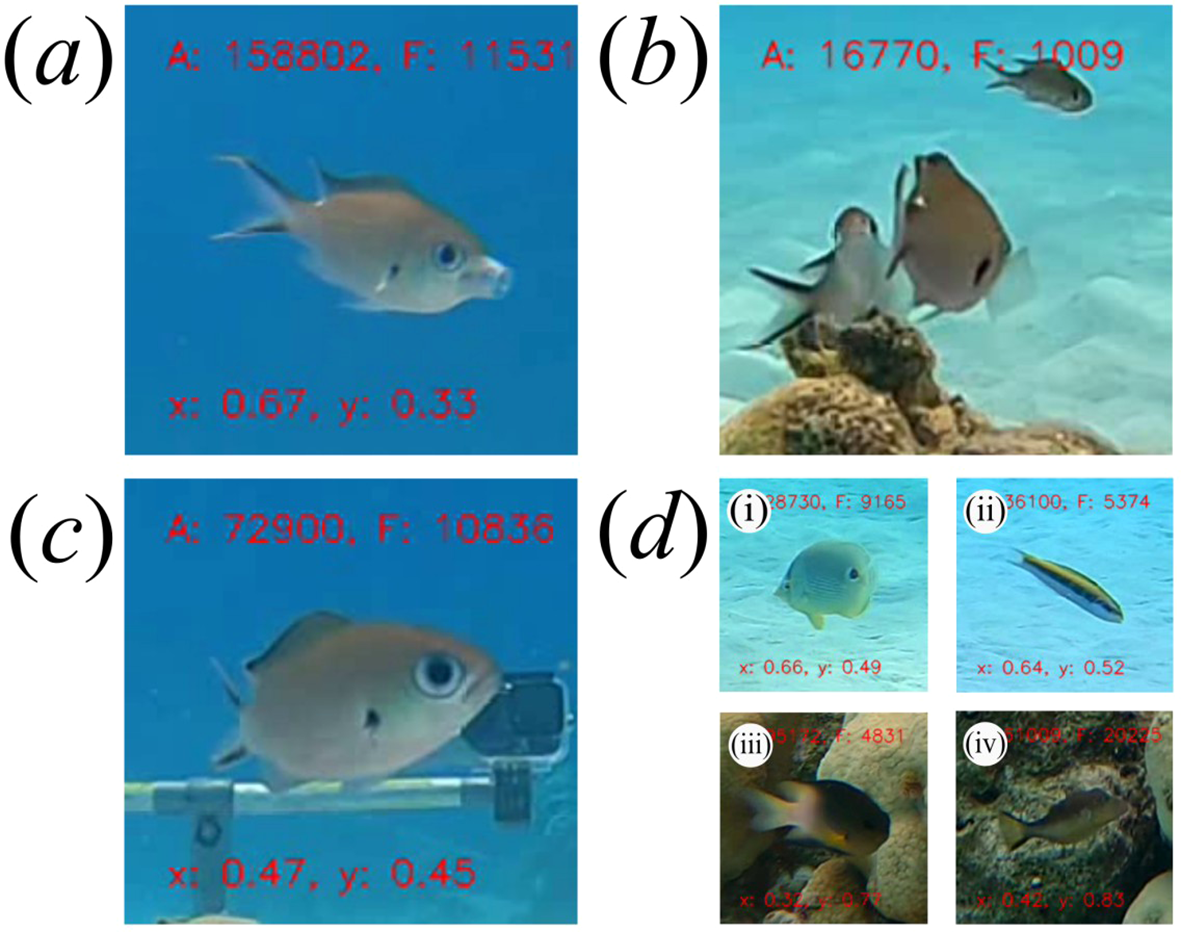
Individual brown chromis behaviour classes used for training the image classification model. (a) Feeding, (b) mouth not visible, (c) not feeding mouth visible, (d) (i-iv) non-chromis.
We wanted to calculate mean per-capita feeding rates of brown chromis aggregations as a function of time. However, whether or not a brown chromis is striking at prey can only be determined in periods when the chromis is oriented such that its mouth is visible. Additionally, in some instances, due to errors in the object detection model, non-chromis fish were tracked, which are not of interest to our study. Therefore, each frame of the tracked chromis video clips was annotated as one of four classes: “feeding”, “not feeding mouth visible”, “mouth not visible” and “non-chromis” (see Figure 1). We labelled each frame of the tracked chromis video clips using a custom annotation tool created in MATLAB (The MathWorks Inc., 2022). To generate a training database for the frame-by-frame behavioral classification model, we extracted all “feeding” frames from the annotated tracked chromis video clips, and one of every five frames for each of the other classes. This resulted in a dataset comprising 173 813 images, divided within each class into training, validation and testing datasets under a 70%, 20%, 10% split, which was used to train the image classification model (“YOLOv8 large” classification model) for 100 epochs (Redmon et al., 2016).
Generating feeding-rate estimates for brown chromis aggregations
To generate per-capita feeding rate estimates for a brown chromis aggregation, we applied the detection, tracking, and behavioral classification steps described above. These model inference steps, as well as model training, were implemented in Python using Google Colab notebooks, executed on an NVIDIA A100 GPU. The model output at this stage provides predictions of the most likely behavioral class for each frame of each tracked chromis video clip. To convert this to estimates of per-capita feeding rates, several post-processing steps were applied. First, tracked chromis video clips shorter than or equal to 20 frames were excluded, as tracked chromis video clips at or below this frame length are often part of the “non chromis” class, and we also excluded any tracked chromis video clips that had 10% or more of its frames with “non-chromis” labelled as the most likely class. This threshold was determined to exclude nearly all non-chromis tracks, while excluding relatively few true chromis tracks.
Secondly, because feeding strikes by chromis species typically last ~30–60 milliseconds (Coughlin and Strickler, 1990), we often observed 2–4 consecutive frames where the most likely class was “feeding”. We therefore counted such consecutive detections of feeding behaviors as one feeding event. Additionally, in rare cases, we observed prolonged jaw extensions, which appeared to be a form of stretching behavior unrelated to feeding. We therefore treated periods of prolonged jaw extensions (> 5 frames) as non-feeding events, and relabeled these frames from “feeding” to “not feeding mouth visible”. After these post-processing steps, we calculate the per-capita feeding rate of chromis as the number of detected feeding events per amount of time when the mouths of chromis were labelled as visible i.e., sum of feeding frames and not feeding mouth visible frames.
Model evaluation and bias correction
We evaluated the precision and recall of the brown chromis detection model on the “test” object detection dataset, comprising 149 images. We also evaluated the precision and recall of the behavior classification model as described by Belcher et al. (2023) on the classification test dataset comprising 24 837 images (557 “feeding”, 5 507 “mouth not visible”, 584 “non-chromis”, and 18 189 “not feeding mouth visible”).
In addition, we generated a dataset of 1 998 tracked chromis video clips for which each frame’s behavior was manually annotated, randomly selected from all 12 deployments and not used for model training or validation. For each video, we labelled each frame as one of the four behavioral classes. This dataset was used to assess bias in feeding rate estimates and evaluate the accuracy of feeding rate estimates. Classification errors (precision and recall< 1) can bias estimates; for example, recall of 0.5 for feeding events with perfect precision would lead to feeding rate estimates 50% lower than the true rate. Moreover, if model performance varies systematically across image features (e.g. bounding box size, background color), it may bias comparisons of feeding rates across contexts. We therefore evaluated how recall and precision for the two behavioral classes relevant to feeding rate, “feeding” and “not feeding mouth visible”, varied with frame-level characteristics affecting image quality or visibility. These included bounding box area (larger for fish closer to the camera), x–y coordinates (higher image quality near the center of the frame), and the median red, green, and blue (RGB) pixel values of the image background (see Supplementary Figure 2). Median RGB values for each frame were calculated from the outer row of pixels from the cropped images to capture background color while excluding the fish.
To assess these sources of bias, we generated classification predictions for each frame in the 1 998 manually annotated tracked chromis video clips and examined how precision and recall varied with the image-level covariates above. Full results are presented in Supplementary Table 1. The most important factor affecting recall was bounding box area: recall approached zero for small boxes and one for large bounding boxes. To avoid high error rates in feeding estimates, we excluded data with bounding box areas below the threshold where feeding recall dropped below 0.5 (<1 451 pixels). Thus, fish that are too far away from the camera, appearing too small in the image to reliably detect feeding events, are excluded from feeding rate calculations.
We then fit logistic regression models to predict precision and recall for the “feeding” and “not feeding mouth visible” classes as a function of frame-level variables, using the dredge function in the MuMIn package in R (Bartoń, 2024) and AIC to select the best models (Supplementary Table 1). These predictions were used to correct per-capita feeding rate estimates according to Equation 1:
where nf and nnfmv are the number of predicted “feeding” and “not feeding mouth visible” frames, respectively, and P and R represent the average precision and recall for each class (indicated by subscripts) over the period in which feeding rate is calculated.
Finally, we evaluated the accuracy of corrected feeding rates as a function of the amount of data used in their calculation. We randomly sampled 10 000 subsets of the 1 998 manually annotated tracked chromis video clips, ranging from 1 to 200 tracks. For each sample, we compared the corrected estimate to the ground-truth feeding rate and calculated the standard deviation of these differences across samples, binned by total duration (in 10-second intervals). This analysis allowed us to quantify how the precision of feeding rate estimates improves with increasing data.
Applying the machine-learning tool
To demonstrate the utility of the pipeline, we used it to investigate predators’ influence on the feeding behavior of brown chromis, in reactive and proactive predator avoidance contexts (Creel, 2018). In the case of reactive predator avoidance behaviors, triggered by the presence of predators, we identified periods from the footage collected in the 12 deployments in which a predator, Caranx ruber (bar jack), swam through the video-recording quadrat set-up, and observed how chromis groups reacted to this. The collective response of chromis to predator encounters was fairly stereotyped, allowing us to categorize chromis group behavior into five states (“feeding normally” before and after predator disturbance, as well as “moving towards”, “hiding in”, and “moving away from” a coral refuge, see Figure 2). For each predator approach, we quantified the mean per-capita feeding rate in each of the five states. Differences in feeding rate among behavioral states were tested using a linear mixed-effects model (function “lmer()” in R) with group behavior category as a fixed effect and deployment as a random intercept, followed by Tukey-adjusted pairwise comparisons to assess differences among states. Feeding rate estimates per behavioral phase for each predator encounter event were treated as independent data points. To compare overall feeding rates during disturbed (“moving towards,” “hiding in,” “moving away”) versus undisturbed (“feeding normally”) periods, we grouped states accordingly and tested for differences using a mixed model with the same random structure. We hypothesized that chromis would feed at reduced rates during predator disturbances relative to undisturbed periods.
Figure 2
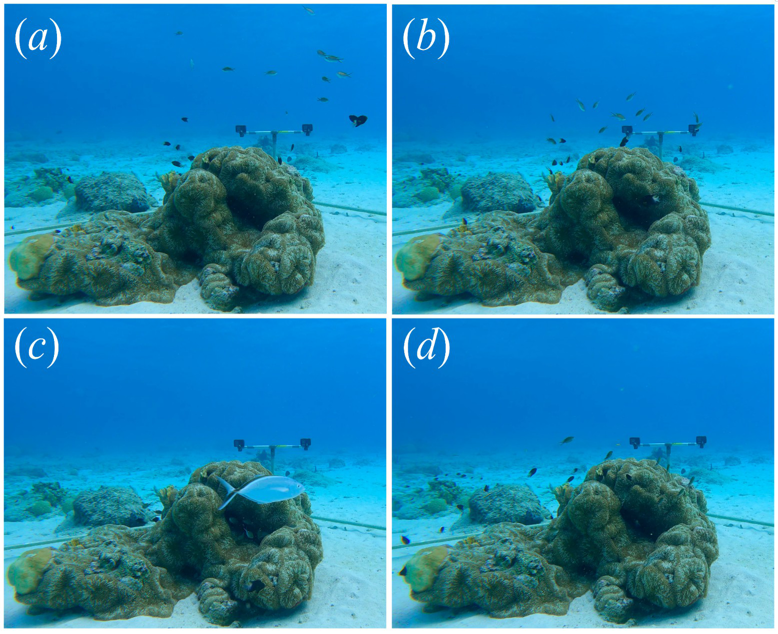
Brown chromis group behaviour categories. (a) Feeding normally (before or after a predator disturbance); (b) moving towards refuge; (c) hiding in refuge (with bar jack predator in view); (d) moving away from refuge.
In the case of proactive predator avoidance (i.e., behavioral responses related to proximity to refuge), we applied the machine-learning pipeline to all 12 one-hour deployments. We evaluated how feeding rates varied along the vertical axis of the water column, hypothesizing that chromis feed more when positioned farther from the coral refuge (i.e., higher in the water column). To test this, we grouped chromis detections within each deployment into quartiles based on their y-pixel (vertical) coordinates and estimated feeding rates for each quartile. To assess systematic variation in feeding activity across depths, we scaled the feeding rate in each quartile by dividing it by the mean feeding rate across all quartiles for that deployment. Thus, values greater than 1 indicate above-average feeding activity at a given depth, while values less than 1 indicate below-average feeding. These deployment-scaled feeding rates for each depth quartile were treated as raw data points. Scaled feeding rates were analyzed using a mixed-effects model with depth quantile as a fixed effect and deployment as a random intercept, followed by Tukey-adjusted post hoc comparisons to test for systematic variation across depths. All data analysis was conducted in R version 4.3.1 (R Core Team, 2023).
Results
Model performance
Bounding box precision and recall values for the object detection model were 0.955 and 0.943, respectively, indicating most chromis in a video are detected and tracked. Errors in the chromis detection model generally only impact estimates of feeding rate by reducing the amount of data used for feeding rate calculations, as undetected and non-tracked chromis are excluded from these calculations.
Performance of the behavioral classification model was high overall. On the 1 998 manually annotated tracked chromis video clips dataset, the precision and recall for feeding events was 0.858 and 0.605, respectively. However, after excluding data with chromis bounding box sizes lower than 1 451 pixels, these values increased to 0.865 and 0.761. Consequently, most feeding events are successfully detected by the model with relatively few false positives. A full description of model performance for all behavioral classes is given in Supplementary Tables 2–4.
After applying the bias correction functions for precision and recall of the “feeding” and “not feeding mouth visible” eq. 1, we found that the precision of the feeding rate estimates scaled with the inverse square root of the amount of seconds of data used in the feeding rate calculation (Figure 3), such that standard deviation of feeding rate estimation error (SDEFR) was, as per Equation 2:
Figure 3
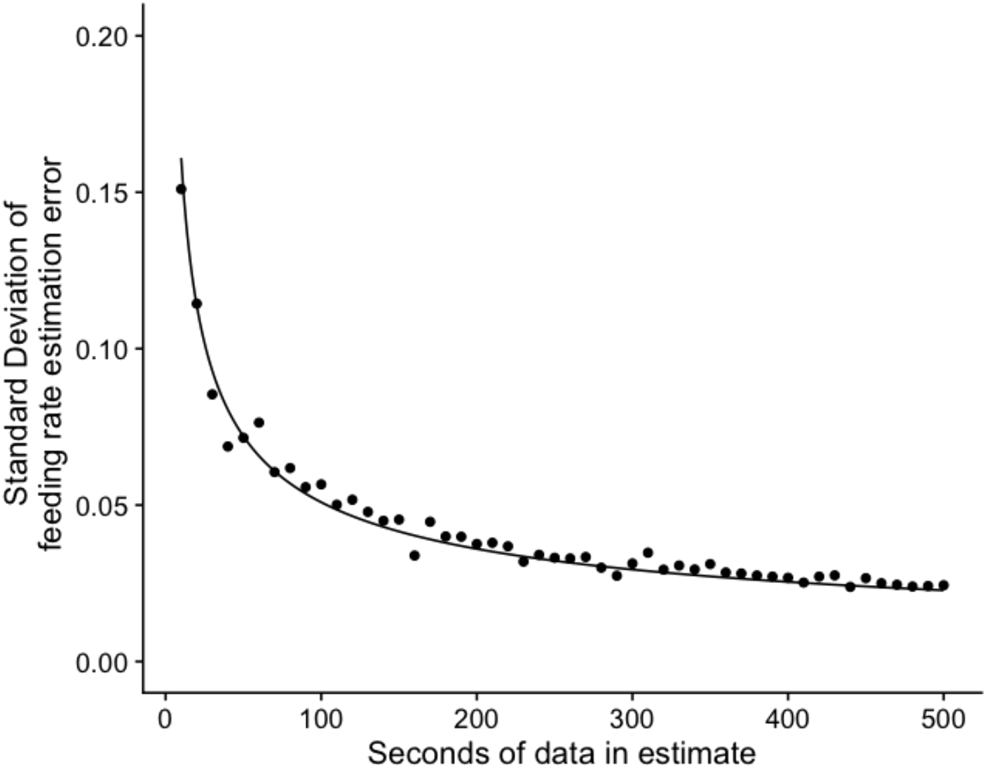
Precision of feeding rate estimates as a function of dataset size. Points depict the standard deviation of the differences between predicted and ground truth feeding rate estimates (SDEFR) as a function of dataset size (number of seconds of tracked fish in the estimate), binned into 10-second intervals (see “Model Evaluation and Bias Correction”). SDEFR scaled with the inverse square root of dataset size (fitted line). For reference, the average per-capita feeding rate of brown chromis in our study was 0.54 (strikes s-1 fish-1).
where n is the number of seconds of data ((“feeding” + “not feeding mouth visible frames”)/60) used in the feeding rate estimate. Thus, our model allows for accurate estimates of chromis strike rates at relatively high temporal resolution (10s to 100s seconds).
Feeding behavior of brown chromis
A total of 31 predator encounters were observed in the field-collected footage, 2.58 ± 2.02 (SD) times per deployment, and were used for analysis. The average total time of disturbance per predator encounter, or the total time spent “moving towards refuge”, “hiding in refuge” and “moving away from refuge”, was 22.71 ± 15.93 (SD) seconds. An example of model predictions of individual brown chromis fish detections and their behaviors, as well as the feeding rate through time of a brown chromis aggregation across the different collective behaviors in a single predator encounter event, is shown in Figure 4.
Figure 4
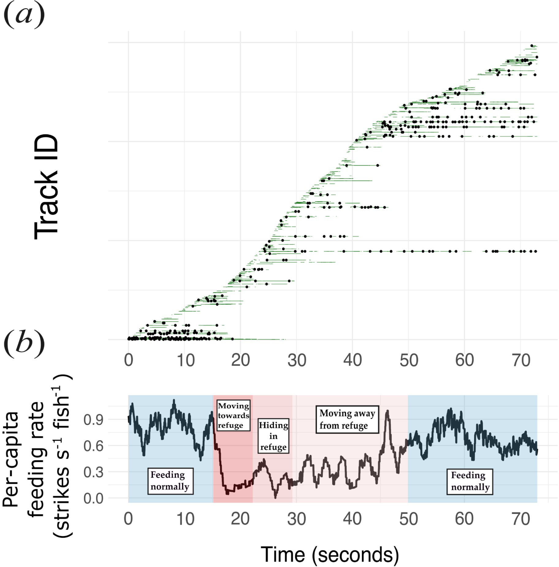
Feeding rates and behaviour of a brown chromis group and its individually tracked members within a predator encounter video. (a) Individually tracked chromis within a single predator-approach video. Each horizontal line represents the full duration of one track, ordered vertically by the first frame in which the track was detected. Tracks do not necessarily correspond to unique fish: new tracks are initiated whenever an existing track is interrupted due to occlusion or temporary detection failure. The symbols and colours along each line indicate the behavioural state assigned at each frame: black dots denote predicted feeding events; green segments indicate frames in which the mouth is visible but not feeding; and white segments indicate frames in which the mouth is not visible and therefore excluded from feeding-rate estimates. (b) Average feeding rate per second (using an 8-second moving window) of a chromis aggregation through time across the five group behaviour phases.
Feeding rate during predator approaches
Feeding rates of Chromis multilineata declined sharply in the presence of predators (Figure 5a). Estimated marginal means from the mixed-effects model (including deployment as a random intercept) showed that feeding rates were highest when fish were feeding normally, both before (0.57 ± 0.05 SE strikes s−1 fish−1) and after (0.54 ± 0.05 SE) predator approaches, and markedly lower when fish were moving away from (0.36 ± 0.05 SE) or towards (0.33 ± 0.05 SE) the refuge, or hiding within it (0.21 ± 0.05 SE). Pairwise comparisons (Tukey-adjusted) indicated that feeding rates during all disturbed behaviors were significantly lower than during normal feeding (p < 0.005 in all cases), while rates before and after predator approaches did not differ (p = 0.98). Feeding rates while hiding were significantly lower than those while moving away from the refuge (p = 0.015), but not significantly different from those while moving towards it (p = 0.066). Overall, mean feeding rates across disturbed stages were roughly half those observed during undisturbed periods (Figure 5b).
Figure 5
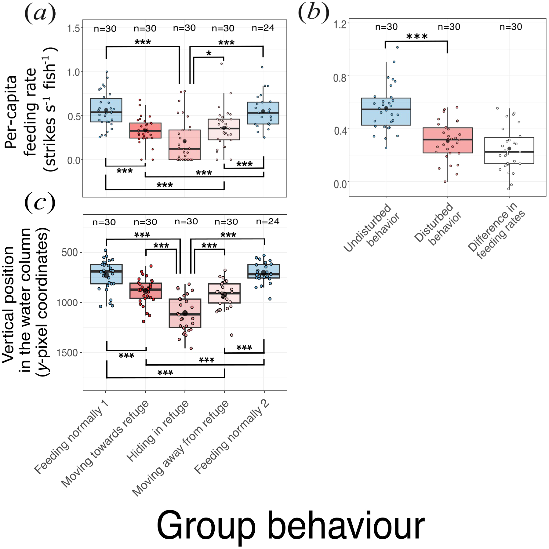
Feeding rate of brown chromis in response to predators. (a) Feeding rate of brown chromis aggregations per group behaviour phase during predator approaches. (b) Feeding rate during disturbed vs. undisturbed behaviours. (c) Vertical position (y-pixel coordinates) of brown chromis aggregations per group behaviour phase during predator approaches. Boxes (coloured by group behaviour) represent the interquartile range, horizontal black lines within correspond to medians, black dots to means, coloured dots to raw data points (coloured by group behaviour), sample size per group is displayed after “n=“ above each box. Raw data points correspond to (within a predator encounter video): (a) average feeding rate for each behavioral phase; (b) average feeding rate for disturbed and undisturbed behaviours, and the difference between these; (c) average y-pixel coordinates for each behavioral phase. Whiskers extend to the maximum and minimum values within 1.5*IQR. Significant differences are indicated by “*” and “***” at p=0.01-0.05 and p=0.000-0.001 level, respectively.
The reductions in feeding rate observed during predator approaches coincided with chromis descending deeper in the water column (Figure 5c). Because the videos were recorded with a single camera, we used the y-pixel coordinate of each chromis detection as a proxy for depth, where higher y-pixel values correspond to lower (deeper) positions within the field of view. On average, chromis occupied the highest positions in the water column during the “feeding normally” stages, both before and after predator approaches (mean y-pixel coordinates: 750 ± 40 SE and 729 ± 42 SE, respectively). They were deepest when “hiding in refuge” (1 134 ± 40 SE), and at intermediate depths when “moving towards” or “moving away from” refuge (908 ± 40 SE and 939 ± 42 SE, respectively). Thus, the depth distribution of chromis closely paralleled the changes in feeding activity observed during predator encounters, with individuals descending towards refuge and reducing feeding when predators approached.
Feeding rate of brown chromis across a vertical profile
Feeding rates of Chromis varied across the vertical depth profile (Figure 6). Deployment-scaled feeding rate (the feeding rate within a depth bin divided by the average feeding rate for that deployment) was substantially higher in the three upper quartiles of the water column than in the lowest quartile (Tukey post-hoc: p < 0.0001). Feeding rates among the three lower depth quantiles (25th–75th) did not differ significantly (p > 0.05). On average, fish in the lowermost portion of the aggregation fed 25–30% less frequently than those at shallower depths.
Figure 6
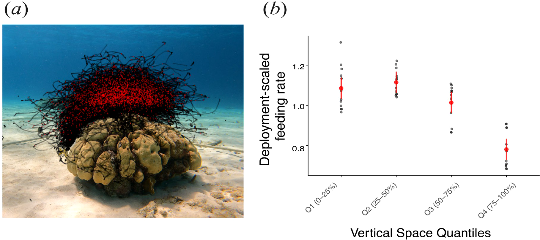
Feeding behaviour of individual brown chromis fish across a vertical profile. (a) Still image of coral-head site 2, with superimposed red and black points corresponding to x and y-axis coordinates of feeding and non-feeding events, respectively, of individual brown chromis within a one-hour deployment. (b) Deployment-scaled feeding rates (feeding rate of each quartile divided by the mean feeding rate across all depth quartiles for the deployment) across the depth quartiles (grey points), where Q1, Q2, Q3 and Q4 correspond to each quartile, ordered from highest to lowest position in the water column; red points and error bars correspond to predicted deployment-scaled means and 95% confidence intervals.
Discussion
Ultimately, understanding how energy flows through ecological systems and predicting how such systems will respond to environmental change depends on knowing the rates at which species interact. While ecological theory often hinges on interaction rates (e.g. feeding, competition, mutualism), these rates are rarely measured directly in the field. Here, we show that automated computer-vision tools can overcome many of the constraints that have long limited behavioral measurements in ecology. By enabling continuous, high-resolution quantification of feeding events, our approach extends the scope of direct behavioral observation to broader spatial and temporal scales, yielding precise, scalable estimates of feeding rates and providing a general framework for quantifying ecological interactions in situ.
Model performance
Importantly, the utility of tools for measuring interaction rates depends on their accuracy. We found that by explicitly modelling and correcting for sources of error in our behavioral classification model, we were able to produce precise and unbiased estimates of feeding rates at fine spatial and temporal scales. Although the classifier was not perfect (recall = 0.76 for feeding events), accounting for how recall and precision varied with frame-level characteristics allowed us to correct for systematic biases in feeding rate estimates. Because individual errors in detecting feeding events tend to average out over time, the accuracy of feeding rate estimates improves with the amount of data used. For example, just 60 seconds of cumulative track data (e.g., 10 fish tracked for 6 seconds each) yielded feeding rate estimates with a standard deviation of errors equivalent to 12% of the mean chromis feeding rate. With 600 seconds of tracked data, this error drops to just 4% of the mean. Thus, even relatively short observation periods can yield precise feeding estimates, and longer periods offer near-ground-truth accuracy, allowing for precise quantification of interaction rates over fine temporal and spatial scales.
Findings from this application
We demonstrated the types of ecological questions that can be addressed with high-resolution measurements of interaction rates by analyzing variation in brown chromis feeding behavior in response to predation risk, both reactive, during predator encounters, and proactive, across vertical gradients of perceived threat. During predator encounters, feeding rates dropped by approximately 50%, consistent with our hypothesis that reactive predator avoidance behavior reduces foraging opportunities. Specifically, chromis feeding rates were significantly higher during undisturbed periods, when fish were dispersed and feeding high in the water column, compared to periods when they were moving towards, hiding in, or moving away from the coral-head refuge. Notably, the reduction in feeding rates in the presence of predators (~50%) was higher than the observed reduction in feeding for chromis distributed in the lowest depth quartile during the full deployments, suggesting the reduction in feeding in periods when a predator is present go beyond the expected reduction in feeding rates due to their proximity to the refuge alone. Perhaps more surprising is that chromis continue to feed at all while actively moving back to the refuge and hiding in close proximity to a predator. This suggests strong selective pressure on planktivores to maintain energy intake even in the face of elevated predation risk.
In addition to reactive responses to predator presence, we observed evidence of proactive risk avoidance, a spatial pattern in feeding behavior that persisted even in the absence of nearby predators. Across all deployments, chromis consistently fed at higher rates when occupying upper regions of the water column. When in the lowest quartile of their distribution (i.e., closest to refuge), chromis fed at rates 20–30% lower than in higher strata. This reduction likely reflects both reduced access to zooplankton, which concentrate higher in the water column due to currents (Hamner et al., 1988; Gove et al., 2016), and increased competition among more tightly aggregated individuals (Alldredge and King, 2009; Orrock et al., 2013). Given that predator approaches were relatively rare and short (~twice per hour, lasting ~20 seconds), this suggests a substantial portion of chromis foraging behavior is constrained by occupying positions in the water column with reduced opportunities for feeding. This pattern is consistent with the concept of a “landscape of fear” (Lima, 1998; Laundré et al., 2001), where prey modify habitat use based on spatial variation in perceived predation risk. While reactive non-consumptive effects result in strong but brief reductions in feeding, proactive responses may exert a more continuous and cumulative influence on energy intake. Chromis may forgo higher foraging rewards higher in the water column in favor of safer, but less productive zones, incurring a steady cost that may outweigh the short-term effects of predator disturbances. Thus, both the frequency of predator encounters and, more importantly, the persistent influence of predators on the spatial distribution of planktivores can reduce the strength of pelagic subsidies to reef communities by altering planktivory rates. These findings underscore the importance of both immediate and anticipatory risk responses in shaping energy transfer from pelagic sources to reef-associated consumers (Morais and Bellwood, 2019; Skinner et al., 2021).
Future applications
Our pipeline opens the door to a wide range of ecological applications where direct measurement of interaction rates has previously been infeasible. Within coral reef ecosystems, it could be used to quantify how rates of planktivory vary across reef zones (e.g., fore reef vs. back reef), between different coral morphologies, or over diel cycles. Such measurements could help test hypotheses about how physical habitat structure modulates foraging behavior and energy flow. When paired with reef-wide surveys of fish abundance, targeted behavioral measurements could also be used to scale up from individual-level feeding to community-level estimates of total planktivory across a reefscape. In addition, by measuring feeding rates across a range of local fish densities, the tool could be used to explore density dependence in planktivory under natural conditions—a question that has been difficult to address in situ. The ram-jaw feeding behavior of Chromis multilineata is widespread among planktivorous damselfishes (Olivier et al., 2017), suggesting that this approach could be readily extended to numerous other species within the Pomacentridae family.
While we implemented the approach for Chromis multilineata, a species whose jaw extensions make feeding events visually distinct, the underlying pipeline is not limited to this behavior or taxon. In essence, the method is transferable to any system where the behavioral classes of interest can be reliably detected by a classification model from static images. In such cases, the same detection, tracking, and bias-correction framework can be directly applied, requiring only retraining of the tracking and classification models on new labelled data. This includes potential applications in laboratory settings or for other visually recognizable behaviors such as courtship or aggression. For interactions that are not visually discernible from single frames and require temporal context, video-based deep learning approaches, such as anchor-free temporal action detection models or transformer-based models, may be required to detect interactions (Vahdani and Tian, 2023). Nonetheless, the core pipeline we present, combining tracking, frame-based classification, and bias correction, offers a robust, generalizable framework for quantifying a diverse range of visually identifiable ecological interactions.
Limitations
An important limitation of our approach in the context of quantifying planktivory is that, due to the large size disparity between planktivorous fish and their zooplankton prey, our pipeline captures only the behavior of the predator, not the identity or size of the prey being consumed. While previous stomach content analyses suggest that brown chromis feed primarily on copepods (comprising ~87% of their diet), copepod species can vary significantly in body size and energy content. This variation makes it difficult to directly convert feeding event rates into biomass or energy flux without additional information on prey identity. To translate behavioral data into estimates of energy transfer or trophic flux, our approach would need to be complemented by concurrent measurements of prey availability and composition, such as paired plankton tows, gut content analysis, or emerging optical tools capable of resolving prey in situ (Lertvilai, 2020; Pollina et al., 2022). Incorporating such data would allow for converting observed feeding rates to biomass or energy fluxes, improving estimates of the ecological consequences of planktivory across reef environments. Importantly, this limitation is specific to predator–prey interactions involving highly size-mismatched species. In other systems, such as mutualisms, competition, or aggression, where interacting species are of comparable size, the identities of both participants may be directly observable, and this constraint may not apply.
Because our classifier detects prey capture attempts rather than successful ingestion, feeding rates may be overestimated if capture success is low. However, for ram-feeding species like Chromis multilineata, prey capture success is generally high (~90%) even against evasive copepods (Coughlin and Strickler, 1990), and is therefore unlikely to introduce substantial bias into feeding rate estimates or comparisons across time or environmental gradients.
Conclusions
Our study demonstrates how machine-learning-based computer vision can be used to directly quantify the rate of ecological interactions in the field, overcoming long-standing challenges in measuring dynamic processes like planktivory. By combining automated detection, tracking, behavioral classification and bias correction, our approach enables scalable, high-resolution estimates of feeding rates in natural conditions. As automated computer vision tools continue to advance, they offer powerful new opportunities to link behavior with ecological function, resolving how individual behaviors scale up to shape ecosystem dynamics.
Statements
Data availability statement
The data presented in the study are deposited in https://figshare.com/articles/dataset/Automated_interaction_rates/29069525, accession number 29069525.
Ethics statement
The requirement of ethical approval was waived by The Head Animal Welfare Body of the University of Amsterdam for the studies involving animals because no animals were handled, as set out in the Dutch Experiments on Animals Act. The studies were conducted in accordance with the local legislation and institutional requirements.
Author contributions
MS: Writing – original draft, Writing – review & editing, Data curation, Formal analysis, Investigation, Methodology, Software, Validation, Visualization. BM: Conceptualization, Data curation, Formal analysis, Funding acquisition, Investigation, Methodology, Project administration, Resources, Software, Supervision, Validation, Visualization, Writing – review & editing.
Funding
The author(s) declared that financial support was received for this work and/or its publication. This research was supported by the Dutch Research Council (NWO grant VI.Vidi.203.085).
Acknowledgments
We thank Lena Faber and Luna Buwalda for their assistance with field work, and Andrew Hein and Abigail Grassick for their feedback on the machine-learning pipeline. The content of this manuscript is available online in the form of a preprint in bioRxiv (Sadde and Martin, 2025; doi: https://doi.org/10.1101/2025.08.05.668677).
Conflict of interest
The authors declared that this work was conducted in the absence of any commercial or financial relationships that could be construed as a potential conflict of interest.
Generative AI statement
The author(s) declared that generative AI was not used in the creation of this manuscript.
Any alternative text (alt text) provided alongside figures in this article has been generated by Frontiers with the support of artificial intelligence and reasonable efforts have been made to ensure accuracy, including review by the authors wherever possible. If you identify any issues, please contact us.
Publisher’s note
All claims expressed in this article are solely those of the authors and do not necessarily represent those of their affiliated organizations, or those of the publisher, the editors and the reviewers. Any product that may be evaluated in this article, or claim that may be made by its manufacturer, is not guaranteed or endorsed by the publisher.
Supplementary material
The Supplementary Material for this article can be found online at: https://www.frontiersin.org/articles/10.3389/fmars.2025.1694767/full#supplementary-material
References
1
Aharon N. Orfaig R. Bobrovsky B.-Z. (2022). BoT-SORT: Robust associations multi-pedestrian tracking ( arXiv). Available online at: http://arxiv.org/abs/2206.14651 (Accessed April 16, 2025).
2
Alldredge A. L. King J. M. (2009). Near-surface enrichment of zooplankton over a shallow back reef: implications for coral reef food webs. Coral Reefs28, 895–908. doi: 10.1007/s00338-009-0534-4
3
Bartoń K. (2024). MuMIn: multi-model inference. Available online at: https://CRAN.R-project.org/package=MuMIn (Accessed April 7, 2025).
4
Belcher B. T. Bower E. H. Burford B. Celis M. R. Fahimipour A. K. Guevara I. L. et al . (2023). Demystifying image-based machine learning: a practical guide to automated analysis of field imagery using modern machine learning tools. Front. Mar. Sci.10. doi: 10.3389/fmars.2023.1157370
5
Bleicher S. S. (2017). The landscape of fear conceptual framework: definition and review of current applications and misuses. PeerJ5, e3772. doi: 10.7717/peerj.3772
6
Brown J. H. Whitham T. G. Morgan Ernest S. K. Gehring C. A. (2001). Complex species interactions and the dynamics of ecological systems: long-term experiments. Science293, 643–650. doi: 10.1126/science.293.5530.643
7
Brown J. S. Laundré J. W. Gurung M. (1999). The ecology of fear: optimal foraging, game theory, and trophic interactions. J. Mammal80, 385–399. doi: 10.2307/1383287
8
Christin S. Hervet É. Lecomte N. (2019). Applications for deep learning in ecology. Methods Ecol. Evol.10, 1632–1644. doi: 10.1111/2041-210x.13256
9
Clare E. L. (2014). Molecular detection of trophic interactions: emerging trends, distinct advantages, significant considerations and conservation applications. Evol. Appl.7, 1144–1157. doi: 10.1111/eva.12225
10
Core Team R. (2023). R: A language and environment for statistical computing (Vienna, Austria). Available online at: https://www.R-project.org/ (Accessed October 13, 2023).
11
Coughlin D. J. Strickler J. R. (1990). Zooplankton capture by a coral reef fish: an adaptive response to evasive prey. Environ. Biol. Fishes29, 35–42. doi: 10.1007/BF00000566
12
Creators C. V. A. T. (2023). ai corporation. Comput. Vision Annotat Tool (CVAT). doi: 10.5281/zenodo.7863887
13
Creel S. (2011). Toward a predictive theory of risk effects: hypotheses for prey attributes and compensatory mortality. Ecology92, 2190–2195. doi: 10.1890/11-0327.1
14
Creel S. (2018). The control of risk hypothesis: reactive vs. proactive antipredator responses and stress-mediated vs. food-mediated costs of response. Ecol. Lett.21, 947–956. doi: 10.1111/ele.12975
15
Desjardins-Proulx P. Laigle I. Poisot T. Gravel D. (2017). Ecological interactions and the netflix problem. bioRxiv, 089771. doi: 10.1101/089771
16
Engel A. Reuben Y. Kolesnikov I. Churilov D. Nathan R. Genin A. (2021). In situ three-dimensional video tracking of tagged individuals within site-attached social groups of coral-reef fish. Limnol Oceanogr Methods19, 579–588. doi: 10.1002/lom3.10444
17
Forbes E. S. Cushman J. H. Burkepile D. E. Young T. P. Klope M. Young H. S. (2019). Synthesizing the effects of large, wild herbivore exclusion on ecosystem function. Funct. Ecol.33, 1597–1610. doi: 10.1111/1365-2435.13376
18
Fox R. J. Bellwood D. R. (2007). Quantifying herbivory across a coral reef depth gradient. Mar. Ecol. Prog. Ser.339, 49–59. doi: 10.3354/meps339049
19
Gove J. M. McManus M. A. Neuheimer A. B. Polovina J. J. Drazen J. C. Smith C. R. et al . (2016). Near-island biological hotspots in barren ocean basins. Nat. Commun.7, 10581. doi: 10.1038/ncomms10581
20
Hamner W. M. Jones M. S. Carleton J. H. Hauri I. R. Williams D. M. (1988). Zooplankton, planktivorous fish, and water currents on a windward reef face: great barrier reef, Australia. Bull. Mar. Sci.42, 459–479. Available online at: https://www.ingentaconnect.com/content/umrsmas/bullmar/1988/00000042/00000003/art00010 (Accessed October 30, 2023).
21
Harris D. J. (2016). Inferring species interactions from co-occurrence data with Markov networks. Ecology97, 3308–3314. doi: 10.1002/ecy.1605
22
Kingsford M. J. MacDiarmid A. B. (1988). Interrelations between planktivorous reef fish and zooplankton in temperate waters. Mar. Ecol. Prog. Ser.48, 103–117. doi: 10.3354/meps048103
23
Laundré J. W. Hernández L. Altendorf K. B. (2001). Wolves, elk, and bison: reestablishing the “landscape of fear” in Yellowstone National Park, U.S.A. Can. J. Zool.79, 1401–1409. doi: 10.1139/z01-094
24
Laundre J. W. Hernandez L. Ripple W. J. (2010). The landscape of fear: ecological implications of being afraid. Open Ecol. J.3. Available online at: http://benthamopen.com/contents/pdf/TOECOLJ/TOECOLJ-3-3-1.pdf (May 13, 2024).
25
Lertvilai P. (2020). The In situ Plankton Assemblage eXplorer (IPAX): An inexpensive underwater imaging system for zooplankton study. Methods Ecol. Evol.11, 1042–1048. doi: 10.1111/2041-210x.13441
26
Lima S. L. (1998). Nonlethal effects in the ecology of predator-prey interactions. Bioscience48, 25–34. doi: 10.2307/1313225
27
Lima S. L. Bednekoff P. A. (1999). Temporal variation in danger drives antipredator behavior: the predation risk allocation hypothesis. Am. Nat.153, 649–659. doi: 10.1086/303202
28
Matassa C. M. Trussell G. C. (2014). Prey state shapes the effects of temporal variation in predation risk. Proc. Biol. Sci.281, 20141952. doi: 10.1098/rspb.2014.1952
29
Morais R. A. Bellwood D. R. (2019). Pelagic subsidies underpin fish productivity on a degraded coral reef. Curr. Biol.29, 1521–1527.e6. doi: 10.1016/j.cub.2019.03.044
30
Myrberg A. A. Brahy B. D. Emery A. R. (1967). Field observations on reproduction of the damselfish, chromis multilineata (Pomacentridae), with additional notes on general behavior. Copeia1967, 819–827. doi: 10.2307/1441893
31
Olivier D. Gajdzik L. Parmentier E. Frédérich B. (2017). Evolution and diversity of ram-suction feeding in damselfishes (Pomacentridae). Org. Divers. Evol.17, 497–508. doi: 10.1007/s13127-017-0329-3
32
Orrock J. L. Preisser E. L. Grabowski J. H. Trussell G. C. (2013). The cost of safety: refuges increase the impact of predation risk in aquatic systems. Ecology94, 573–579. doi: 10.1890/12-0502.1
33
Peacor S. D. Werner E. E. (2001). The contribution of trait-mediated indirect effects to the net effects of a predator. Proc. Natl. Acad. Sci. U S A98, 3904–3908. doi: 10.1073/pnas.071061998
34
Pollina T. Larson A. G. Lombard F. Li H. Le Guen D. Colin S. et al . (2022). PlanktoScope: Affordable modular quantitative imaging platform for citizen oceanography. Front. Mar. Sci.9. doi: 10.3389/fmars.2022.949428
35
Post D. M. (2002). Using stable isotopes to estimate trophic position: models, methods, and assumptions. Ecology83, 703–718. doi: 10.1890/0012-9658(2002)083[0703:USITET]2.0.CO;2
36
Preisser E. L. Bolnick D. I. Benard M. F. (2005). Scared to death? The effects of intimidation and consumption in predator–prey interactions. Ecology86, 501–509. doi: 10.1890/04-0719
37
Redmon J. Divvala S. Girshick R. B. Farhadi A. (2016). You only look once: Unified, real-time object detection. Proc. IEEE Comput. Soc Conf. Comput. Vis. Pattern Recognit., 779–788. doi: 10.1109/CVPR.2016.91
38
Rempel H. S. Siebert A. K. Van Wert J. C. Bodwin K. N. Ruttenberg B. I. (2022). Feces consumption by nominally herbivorous fishes in the Caribbean: an underappreciated source of nutrients? Coral Reefs41, 355–367. doi: 10.1007/s00338-022-02228-9
39
Robinson J. P. W. Benkwitt C. E. Maire E. Morais R. Schiettekatte N. M. D. Skinner C. et al . (2024). Quantifying energy and nutrient fluxes in coral reef food webs. Trends Ecol. Evol.39, 467–478. doi: 10.1016/j.tree.2023.11.013
40
Sadde M. Martin B. T. (2025). Automated quantification of ecological interactions from video. bioRxiv. [Preprint]. doi: 10.1101/2025.08.05.668677
41
Sheriff M. J. Krebs C. J. Boonstra R. (2011). From process to pattern: how fluctuating predation risk impacts the stress axis of snowshoe hares during the 10-year cycle. Oecologia166, 593–605. doi: 10.1007/s00442-011-1907-2
42
Skinner C. Mill A. C. Fox M. D. Newman S. P. Zhu Y. Kuhl A. et al . (2021). Offshore pelagic subsidies dominate carbon inputs to coral reef predators. Sci. Adv.7. doi: 10.1126/sciadv.abf3792
43
Symondson W. O. C. (2002). Molecular identification of prey in predator diets. Mol. Ecol.11, 627–641. doi: 10.1046/j.1365-294x.2002.01471.x
44
The MathWorks Inc (2022). MATLAB version: 9.13.0 (R2022b) (Massachusetts: The MathWorks Inc). Available online at: https://www.mathworks.com (Accessed June 22, 2024).
45
Vahdani E. Tian Y. (2023). Deep learning-based action detection in untrimmed videos: A survey. IEEE Trans. Pattern Anal. Mach. Intell.45, 4302–4320. doi: 10.1109/TPAMI.2022.3193611
46
Villon S. Iovan C. Mangeas M. Vigliola L. (2022). Confronting deep-learning and biodiversity challenges for automatic video-monitoring of marine ecosystems. Sensors, 22. doi: 10.3390/s22020497
47
Zanette L. Y. White A. F. Allen M. C. Clinchy M. (2011). Perceived predation risk reduces the number of offspring songbirds produce per year. Science334, 1398–1401. doi: 10.1126/science.1210908
Summary
Keywords
computer vision, interaction rate, machine learning, non-consumptive effects (NCEs), planktivory, predation
Citation
Sadde M and Martin BT (2026) Automated quantification of ecological interactions from video. Front. Mar. Sci. 12:1694767. doi: 10.3389/fmars.2025.1694767
Received
28 August 2025
Revised
14 November 2025
Accepted
01 December 2025
Published
16 January 2026
Volume
12 - 2025
Edited by
Elva G. Escobar-Briones, National Autonomous University of Mexico, Mexico
Reviewed by
Julian Lilkendey, University of Bremen, Germany
Emily Kane, University of Louisiana, United States
Updates
Copyright
© 2026 Sadde and Martin.
This is an open-access article distributed under the terms of the Creative Commons Attribution License (CC BY). The use, distribution or reproduction in other forums is permitted, provided the original author(s) and the copyright owner(s) are credited and that the original publication in this journal is cited, in accordance with accepted academic practice. No use, distribution or reproduction is permitted which does not comply with these terms.
*Correspondence: Benjamin T. Martin, b.t.martin@uva.nl
Disclaimer
All claims expressed in this article are solely those of the authors and do not necessarily represent those of their affiliated organizations, or those of the publisher, the editors and the reviewers. Any product that may be evaluated in this article or claim that may be made by its manufacturer is not guaranteed or endorsed by the publisher.