Abstract
Phytoplankton are fundamental components of marine ecosystems and play a critical role in global biogeochemical cycles. Efficient monitoring of marine phytoplankton is crucial for assessing ecosystem health, forecasting harmful algal blooms and sustainable marine management. The integration of high-throughput imaging sensors like FlowCam technology with artificial intelligence (AI) for image recognition has revolutionized phytoplankton monitoring, enabling rapid and accurate class identification. This study introduces an automated image classification workflow designed to improve speed, accuracy and scalability of phytoplankton identification. By leveraging convolutional neural networks (CNNs), the system enhances performance while reducing reliance on traditional, labor-manual identification methods.
1 Introduction
Phytoplankton plays a pivotal role in both marine and freshwater ecosystems. They provide over 45 percent of the global net primary production, play a pivotal role in the global carbon and nutrient cycles and they fuel entire aquatic foodwebs through their photosynthetic activity (Ducklow et al., 2001; Hays et al., 2005; Pierella Karlusich et al., 2020). Moreover, phytoplankton has the ability to quickly respond to environmental and anthropogenic disturbances through their short generation times. The Water Directive Framework and the Marine Strategy Framework Directive recognize phytoplankton as an indicator for monitoring aquatic ecosystem health (Tett et al., 2008; European Commission, 1999).
Marine and freshwater plankton represent a highly diverse group of organisms, both taxonomically and morphologically, spanning numerous phyla and tens of thousands of species (Sournia et al., 1991; De Vargas et al., 2015). They are generally small in size, going from less than 1 µm up to 1 mm (Winder and Sommer, 2012). Traditionally, phytoplankton identification has relied on expert taxonomists manually classifying specimens under a microscope. This process is not only time-consuming and resource-intensive but also demands highly skilled specialists to distinguish subtle morphological differences between taxa (Benfield et al., 2007).
To address these issues, researchers are increasingly adopting specially designed high-throughput digital imaging systems. These systems, such as the Video Plankton Recorder (Sournia et al., 1991; Ollevier et al., 2022) and the FlowCam (Sieracki et al., 1998), are employed both in situ and in laboratory settings, respectively. These next-generation imaging systems significantly speed up analysis time in the lab by capturing thousands of particles in a matter of minutes. While these systems generate vast volumes of plankton image data, the lack of automated, reliable classification techniques means that manual image classification is still necessary, creating a bottleneck in the processing workflow (Kerr et al., 2020; Sosa-Trejo et al., 2023). Recent studies have turned to automated methods, particularly Convolutional Neural Networks (CNNs) (LeCun et al., 2015; Krizhevsky et al., 2012), to perform plankton image classification Luo et al. (2018); Dunker et al. (2018); Lumini and Nanni (2019); Guo et al. (2021); Henrichs et al. (2021); Kraft et al. (2022a); Immonen (2025). For instance, models developed using datasets from the Finnish Environment Institute (SYKE) have demonstrated strong performance across multiple phytoplankton taxa (Kraft et al., 2022a). In this study, we further investigate cross-dataset generalization by retraining our model and the SYKE model on each other’s datasets, enabling a direct comparison of performance and transferability across imaging conditions. This approach highlights both the robustness of CNN-based classifiers and their potential for broader applicability in automated plankton monitoring.
Although other methods to classify plankton exist—including traditional feature-engineering approaches using shape, texture, color, or local descriptors combined with classifiers such as SVM or random forests (Blaschko et al., 2005; Sosik and Olson, 2007; Zheng et al., 2017), and hybrid methods that combine handcrafted features with CNN-based features (Orenstein and Beijbom, 2017; Keçeli et al., 2017). A great advantage of CNN vs hand-crafted approaches is that since CNN adopt effective representations of the original image, they require a very small amount of pre-processing Lumini and Nanni (2019). For the past decade, the popularity has rapidly shifted from feature engineering towards feature learning, where instead of finding the features, they are learned for the classification task. This removes the process of crafting and selecting sufficient features entirely.
Furthermore also object detection pipelines for multi-specimen images using models like YOLO or Faster R-CNN (Pedraza et al., 2018; Soh et al., 2018), however because the FlowCam imaging system used in this study produces single-specimen images that are already centered and cropped, there is no need for an object detection step, such as YOLO, simplifying the processing pipeline and allowing direct classification.
In addition to CNNs, transformer-based architectures such as Vision Transformers (ViTs) and Swin Transformers have recently demonstrated state-of-the-art performance in various image recognition tasks, including plankton classification (Kyathanahally et al., 2022; Maracani et al., 2023). However, Immonen (2025) illustrates that the EfficientNetV2-B0 CNN architecture (Tan and Le, 2021) outperforms other CNNs and transformers for plankton recognition from CytoSense Dubelaar et al. (1999). This performance advantage is likely due to the relatively small size and lower visual complexity of plankton images compared to natural image datasets, which reduces the need for the global attention modeling that transformers excel at.
Moreover, CNNs such as EfficientNetV2-B0 are considerably more computationally efficient than transformer-based models, requiring fewer parameters and less memory, making them easier to train on limited hardware resources and faster to deploy for large-scale image processing workflows. Given these considerations, and the strong empirical results reported for plankton data, we opted for a pure CNN approach with the EfficientNetV2-B0 architecture.
Despite the promising performance of deep learning on phytoplankton images, several challenges remain (Lumini and Nanni, 2019; Eerola et al., 2024). First, the amount of labeled data available for training is limited. This limitation is twofold: (a) expert knowledge is required for accurate labeling, as the diversity of phylogenetic groups is large and morphological differences between certain taxa can be minimal; and (b) rare species are underrepresented due to their natural occurrence and sampling bias, leading to substantial class imbalance. In addition, variations in image quality—arising from different instruments, lighting conditions, or focus—can introduce uncertainties in both expert annotation and automated classification.
In this study, we leverage a long-term archive of phytoplankton images from the Belgian Part of the North Sea (BPNS), collected as part of the LifeWatch marine observatory. From this archive, we curated a systematically balanced dataset of 95 common taxa, capturing the natural diversity of the BPNS and minimizing class imbalance and temporal drift. Using this dataset, we developed a high-performance CNN classifier (EfficientNetV2-B0) capable of predicting the five most probable taxa, achieving 86.3% top-1 accuracy and 98.8% top-5 accuracy. The classifier and dataset are fully integrated into the iMagine infrastructure and available as a module in the iMagine Marketplace1, providing flexible tools for training, testing, and deployment.
The key contributions of this work are fourfold. First, the creation of a long-term, balanced, and phylogenetically diverse phytoplankton dataset. Second, the development of an efficient CNN-based classifier that achieves state-of-the-art performance on plankton images. Third, the demonstration of model transferability through retraining on an independent dataset (SYKE), showing strong cross-dataset generalization. Finally, the integration into a modular platform facilitates practical adoption, enabling streamlined workflows for automated plankton image analysis. Collectively, these contributions advance both the methodological and practical capabilities in the field of plankton monitoring.
2 Materials and methods
In this section, we describe the data acquisition and image processing procedures, including preprocessing, segmentation, classification, and postprocessing for the accurate identification of 95 classes of phytoplankton using convolutional neural networks (CNNs).
As illustrated in Figure 1, samples were collected aboard the research vessel Simon Stevin. The pipeline then splits: vessel metadata, including GPS coordinates and sampling times, are recorded, while water samples are analyzed with the FlowCam. The FlowCam generates raw image collages, two.txt files containing laboratory parameters, and one.lst file. These outputs are processed in-house using a Python pipeline to extract individual Regions of Interest (ROIs) and store them in an internal imaging database.
Figure 1
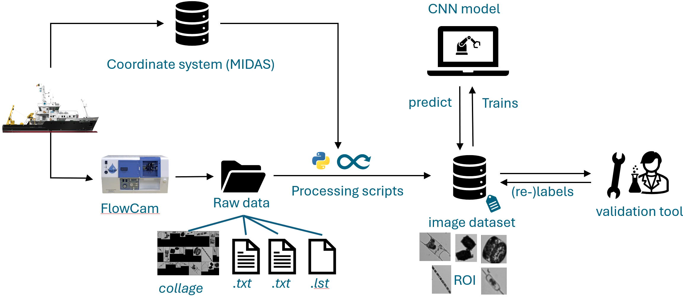
Schematic overview of the FlowCam data acquisition and processing workflow. The process begins with the research vessel Simon Stevin collecting plankton samples. The pipeline then splits: vessel metadata (including GPS coordinates and sampling times) are recorded, while plankton samples are analyzed with the FlowCam. The FlowCam produces raw image collages, two.txt files containing laboratory parameters, and one.lst file. These raw outputs are processed in-house using a Python pipeline to extract individual Regions of Interest (ROIs) and store them in an internal imaging database. Initially, ROIs are manually annotated to create a labelled dataset, which is then used to train a convolutional neural network classifier. The classifier predicts labels for new incoming images, which are subsequently validated, allowing the image dataset to continuously grow over time.
Initially, the ROIs are manually annotated to create a labelled dataset (Figure 1). This dataset is then used to train a CNN classifier, which predicts labels for incoming images. Predicted images are subsequently validated, allowing the dataset to continuously grow over time. This workflow ensures both high predictive accuracy and efficient large-scale processing of FlowCam data.
2.1 Data acquisition
Details of data collection in the field are described in (Lagaisse et al., 2025), and laboratory sample processing protocols and pipelines are described in (Lagaisse, 2024). Briefly, time series are built as part of the LifeWatch marine observatory in the Belgian Part of the North Sea (BPNS), providing a long-term, systematic record of microphytoplankton communities. Sampling is conducted regularly at several fixed stations using the RV Simon Stevin. Specifically, a grid of nine coastal stations is sampled monthly, while eight offshore stations are sampled on a seasonal basis, capturing both spatial and temporal variability in phytoplankton communities.
Samples are collected on board using an Apstein net with a 55 µm mesh size and preserved in Lugol’s iodine solution to maintain cellular integrity. In the laboratory, samples are analyzed using a VS-4 FlowCAM system (Fluid Imaging Technologies) at 4X magnification, targeting particles in the 55–300 µm size range. The FlowCAM is an automated high-throughput imaging system that combines the principles of flow cytometry, microscopy, and digital imaging to generate high-resolution images of individual particles in liquid samples. This technology allows rapid acquisition of thousands of particles per run while preserving morphological details important for taxonomic identification.
Since May 2017, this workflow has generated approximately 300,000–400,000 annotated particle images annually, contributing to a continuously expanding archive of quality-controlled biodiversity data.
2.2 Image and raw output data preprocessing
Raw FlowCam output data consist of image collages and several.txt files containing laboratory-based parameters (e.g., fluid volume imaged, run time, number of images captured, and basic image measurements such as equivalent spherical diameter, ESD). The VisualSpreadsheet software provided by the manufacturer was used solely for FlowCam operation and data acquisition during the laboratory run. Raw and binary images are not stored; instead, only the collages created at the end of each run are retained and used for downstream processing.
As illustrated in Figure 1, the raw data are processed through an in-house developed Python-based pipeline maintained by the Flanders Marine Institute (VLIZ) as part of the LifeWatch observatory. VLIZ is a marine research and data infrastructure institute that coordinates a marine observatory network, data management systems, and computational services for marine science as part of the Belgian contribution to LifeWatch. Within this framework, the LifeWatch programme performs monthly sampling at predefined stations in the Belgian Part of the North Sea (BPNS) to monitor phytoplankton dynamics using the FlowCam VS-4 imaging system, as described in (Lagaisse et al., 2025).
The preprocessing workflow begins by parsing FlowCam run directories containing the image collages and metadata files (.lst,.ctx, and run summaries). Individual Regions of Interest (ROIs) are extracted from the image collages based on pixel coordinates recorded in the raw list files, using custom Python code. Each ROI is cropped while preserving the original background and then subjected to automated integrity checks (e.g., verifying coordinate validity and completeness). Image-level metadata are harmonized with contextual sample information (e.g., sampling station, time, flowcell parameters) retrieved from the MIDAS environmental database.
Processed images and their associated metadata are uploaded to MongoDB, an internal VLIZ database designed for large-scale imaging data. From this database, trained convolutional neural network (CNN) classifiers predict taxonomic labels, which are subsequently validated by experts via the in-house annotation tool. The database maintains a complete history of both machine and human annotations, allowing high-quality, expert-validated classifications to be propagated as ground truth for future training iterations. Aggregated results are automatically converted to taxon densities (cells L−1) and visualized on the LifeWatch FlowCam RShiny data explorer (https://rshiny.vsc.lifewatch.be/flowcam-data/).
Although the VLIZ–LifeWatch infrastructure provides computational advantages and facilitates high-throughput processing, a similar dataflow can be implemented externally using the EcoTaxa platform2 (Irisson et al., 2022; Picheral et al., 2010). However, EcoTaxa currently relies on feature-based classification, whereas the VLIZ pipeline supports full end-to-end CNN training, model iteration, and integration with metadata systems, resulting in higher flexibility and improved predictive accuracy. Nonetheless, the EcoTaxa pipeline can still be used as an annotation and validation tool while CNN-based classification is performed externally.
2.3 Dataset creation
The dataset used for training the classifier comprises 337,567 images of phytoplankton and related particles, grouped into 95 taxonomic classes. Samples were collected within the framework of the Belgian LifeWatch Research Infrastructure, during monthly (coastal) and seasonal (offshore) multidisciplinary campaigns in the Belgian Part of the North Sea (BPNS) aboard the Simon Stevin.
As described in Section 2.2, the raw FlowCam image collages and corresponding metadata files were parsed and processed via the in-house VLIZ Python pipeline to extract individual Regions of Interest (ROIs). The resulting cropped single-object images were stored in an internal imaging database together with metadata such as sampling station, time, and environmental parameters.
Image annotation was performed using in house validation-tool developed at the Flanders Marine Institute. Each image was first predicted by a preliminary CNN classifier and subsequently validated or corrected by trained experts. Annotations were performed at the lowest reliable taxonomic level, typically genus or species, using reference images and the World Register of Marine Species (WoRMS) to ensure taxonomic consistency (AphiaID’s). The final validated labels form the ground truth for model training and ongoing database updates.
To ensure a balanced and practical representation of each class, a minimum of 100 and a maximum of 8,800 images per class were retained. This range ensured sufficient training samples while preventing over-representation of dominant taxa. The resulting dataset was randomly divided into standard splits: 80% for training, 10% for validation, and 10% for testing. An overview of the class distribution is shown in Figure 2.
Figure 2
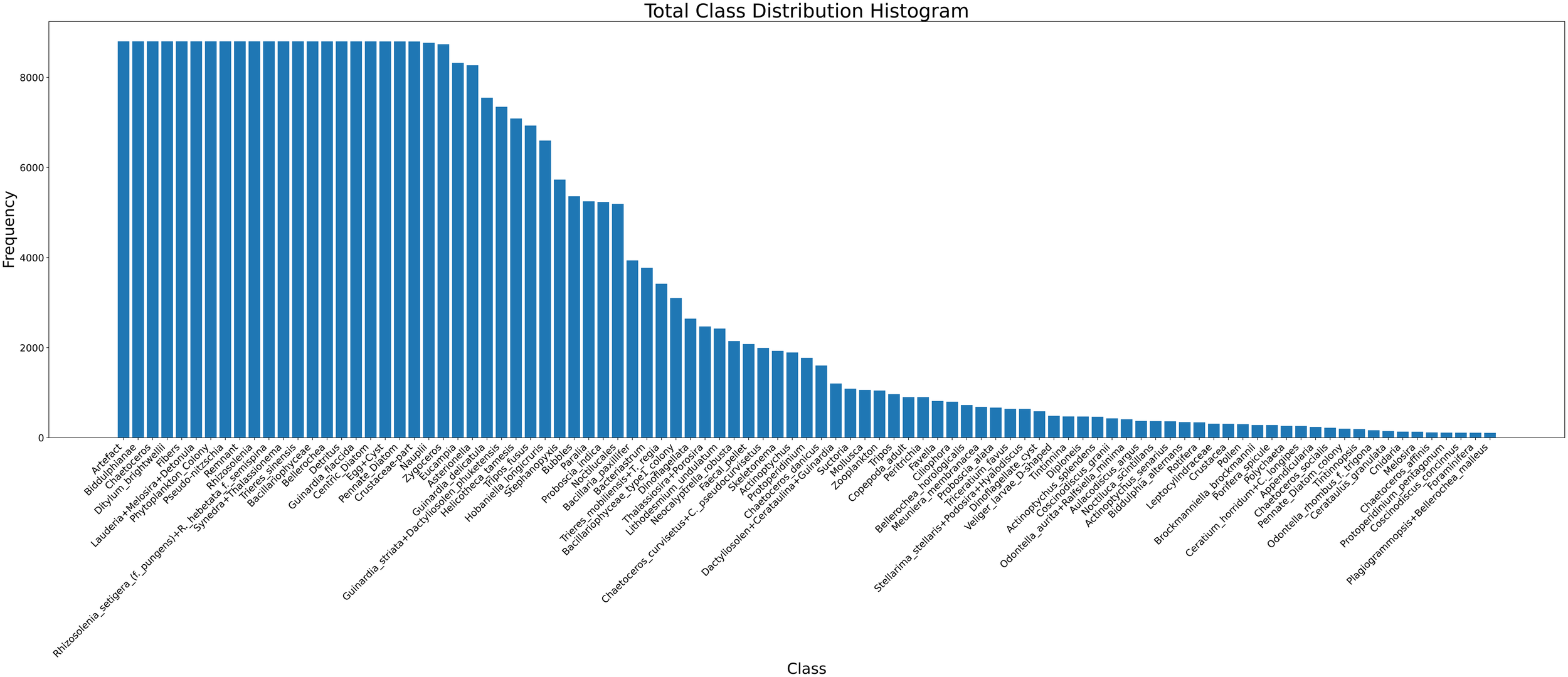
Histogram showing the class distribution across the full phytoplankton dataset.
The fully annotated dataset is openly available on Zenodo (LifeWatch observatory data: phytoplankton annotated training set by FlowCam imaging in the Belgian Part of the North Sea), under the Creative Commons Attribution 4.0 International License (CC BY 4.0).
2.4 Automated image classification
2.4.1 Conceptual overview
The workflow for phytoplankton classification can be divided into two main branches: training a new model or predicting with an existing one (Figure 3). While it is possible to work locally, in this study we leveraged the iMagine platform3, which provides imaging data and AI services for aquatic science. The platform enables scientists to train and deploy AI models for custom use cases, for example, without requiring extensive AI expertise and offering tools that cover the entire machine learning process from image annotation to model monitoring in production.
Figure 3
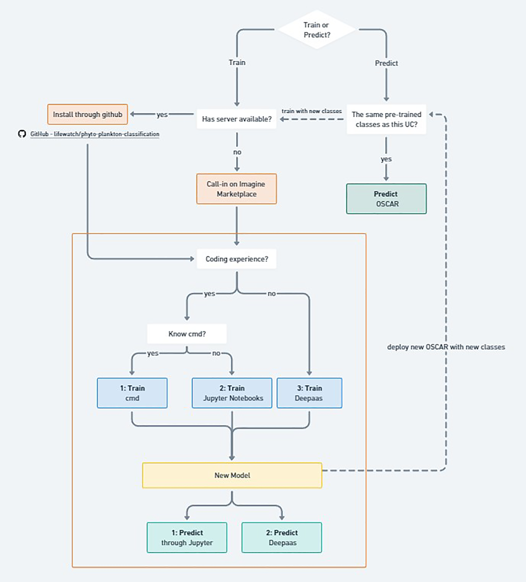
Flowchart illustrating the different methods to (re-)train the model predict phytoplankton classes. Orange square illustrating the part that happens on the iMagine marketplace.
For prediction, the user first checks whether the model’s trained taxa align with the desired set of classes. If they do, predictions can be performed locally by installing the GitHub package4, via the iMagine marketplace using Jupyter or DEEPaaS, or directly through OSCAR (Open Source Serverless Computing for Data-Processing Applications) Pérez et al. (2019), a serverless framework for managing containerized data-processing applications on Kubernetes. If additional classes are required, a new model must be trained and deployed as an updated OSCAR service.
Training can be performed either locally, using the public GitHub repository, or in the cloud via iMagine’s Interactive Development Environments. In both cases, the choice of interface depends on the user’s coding experience: command-line users can train via terminal, intermediate users via Jupyter Notebooks, and those without coding experience via the DEEPaaS API Garcíıa (2019). Regardless of the approach, the result is a trained model ready for prediction through Jupyter, DEEPaaS, or deployment in OSCAR.
The operational pipeline in OSCAR involves three main steps. First, input images are uploaded to an object storage system (based on MinIO MinIO (2020)), which automatically triggers the classifier service. Second, the classifier processes the images using the trained phytoplankton model to identify and categorize taxa from microscope imagery. Finally, the inference results are stored back in the object storage system for retrieval and downstream analyses.
2.4.2 Model architecture
The model architecture of the plankton classifier is based on EfficientNetV2B0, a deep convolutional neural network known for its use of residual connections to facilitate the training of very deep networks. EfficientNetV2B0 is part of the EfficientNetV2 family designed by the Google Brain team (Tan and Le, 2021). We initialized the model with ImageNet weights Deng et al. (2009) and modified the final classification layer to a dense softmax layer matching the number of phytoplankton classes. The full implementation, including training scripts and preprocessing routines, is publicly available on the public GitHub repository.
2.4.3 Network training
Training details are summarized in Table 1. Model training was performed on a Linux system (kernel version 5.15.0-125-generic) equipped with an x86–64 CPU and an NVIDIA Tesla V100-PCIE-32GB GPU (34.07GB VRAM). Training was conducted using TensorFlow 2.19 Chollet et al. (2015) with CUDA 12.1 and cuDNN 8.9.2 in a Python 3.11.11 environment.
Table 1
| Technical information | |
|---|---|
| Operating System | Linux (kernel 5.15.0-125-generic) |
| CPU | x86 64 |
| GPU | NVIDIA Tesla V100-PCIE-32GB (34.07 GB VRAM) |
| Framework | TensorFlow 2.19 Chollet et al. (2015) |
| CUDA/cuDNN | CUDA 12.1, cuDNN 8.9.2 |
| Python | 3.11.11 |
| Training parameters | |
| Dataset size | 337,567 images |
| Train/Validation/Test split | 270,020/33,718/33,829 (80/10/10%) |
| Data handling | Keras Sequence (on-the-fly loading, resizing, normalization) |
| Normalization | RGB mean and std from training set |
| Batch size | 16 |
| Optimizer | Custom Adam |
| Initial learning rate | 0.001 |
| Learning rate schedule | Decay by factor 0.1 at 70% and 90% of epochs |
| Epochs | 20 |
| Regularization | L2 with weight 0.0001 |
AI model training details.
The training pipeline encompasses data preparation, model training, and performance monitoring. The official training, validation, and test splits are included in the Zenodo dataset. This comprises 337,567 images, split into training (270,020; 80.0%), validation (33,718; 10.0%), and test (33,829; 10.0%) sets.
During training, data batches are generated using a custom Keras Sequence that loads, resizes, and normalizes images on the fly. The RGB mean and standard deviation are computed from the training set and used for normalization during training and evaluation. This approach ensures efficient memory use and supports multiprocessing safely during training.
Training was performed using a custom Adam optimizer with an initial learning rate of 0.001 and a batch size of 16 images. The model was trained for 20 epochs with a step-wise learning rate schedule, decaying the learning rate by a factor of 0.1 at 70% and 90% of the total epochs. Additionally, L2 regularization with a weight of 0.0001 was applied to mitigate overfitting.
One possible approach to address class imbalance is to assign class-specific weights to the optimizer (see, e.g., cost-sensitive learning Thai-Nghe et al. (2010)). However, following the approach of Kraft et al. (2022a), this method was not applied here to avoid reducing the model’s generalizability to datasets with different class proportions.
2.5 Model output
The classifier produces a ranked list of the top five predicted phytoplankton classes for each input image, accompanied by their associated confidence scores. These scores represent the model’s certainty in each prediction and are derived from the softmax probabilities of the final classification layer.
Providing the top five predictions allows users to consider multiple plausible identifications rather than relying solely on the highest-probability class. This approach is particularly valuable for ecological datasets, where morphological similarities between taxa can introduce ambiguity.
To improve reliability, a probability threshold can be applied to filter low-confidence classifications, a method widely used in automated plankton analysis Kraft et al. (2022a); Faillettaz et al. (2016); Luo et al. (2018). Only predictions with confidence scores above this threshold are retained, reducing the number of uncertain identifications.
Providing the top five predictions allows users to consider multiple plausible identifications rather than relying solely on the highest-probability class. This is especially useful in ecological datasets where visual similarities between classes can introduce ambiguity. The confidence scores help assess the reliability of each prediction and guide further expert verification or automated downstream analyses.
2.6 Model performance evaluation
The model was compiled using categorical cross-entropy as the loss function, suitable for multi-class classification where each image belongs to a single phytoplankton class. While training accuracy was monitored to track convergence and detect potential overfitting, it alone does not provide a complete picture of performance, particularly for imbalanced ecological datasets.
To obtain a comprehensive evaluation, several complementary analyses were conducted on the independent test set, structured according to global and class-specific performance:
Overall Performance Evaluation
-
Top-K accuracy (K = 1 and 5): Evaluates whether the correct class is among the model’s top-K predicted probabilities. Provides insight into overall ranking behavior and robustness when visually similar taxa are present.
-
Grouped metric breakdown: Precision, recall, and F1-scores were computed using micro-, macro-, and weighted-averaging strategies. This analysis captures both overall trends and the influence of class imbalance.
-
Grouped class frequency analysis: Species were binned according to the number of available training samples. Top-1 and Top-5 accuracies were evaluated within each bin to quantify how sample abundance affects generalization.
-
Overall probability threshold analysis: Assessed the effect of varying the minimum probability threshold on prediction accuracy and coverage, characterizing the trade-off between confidence and inclusiveness.
Class-Specific Performance Evaluation
-
Per-class confusion analysis: Normalized confusion matrices were generated to visualize per-class prediction behavior. Standard and zero-diagonal matrices highlight correct predictions and inter-class misclassifications, respectively.
-
Class-specific metric summary: Precision, recall, and F1-score were calculated individually for each class, providing a detailed overview of reliability across taxa.
-
Probability threshold analysis per class: Explored the effect of confidence thresholds on top1 predictions for each class, showing how increasing the cutoff affects the proportion of correct predictions and retained samples.
This structured approach ensures that both global trends and detailed class-level behaviors are captured, providing a transparent and comprehensive assessment of model performance.
2.7 Model benchmark
To evaluate the generalization ability of our model, we benchmarked it against the publicly available Baltic Sea phytoplankton dataset (Kraft et al., 2022b), originally described in (Kraft et al., 2022a). This dataset contains approximately 63,000 labeled images across 50 phytoplankton classes, along with an evaluation set of about 150,000 images collected from natural communities throughout an annual cycle.
We retrained both architectures on each other’s datasets without changing the model designs, hyperparameters, or preprocessing pipelines. Specifically, we conducted two complementary experiments:
-
External-to-Local Test: Retraining the published model from Kraft et al. (2022b) on our dataset to assess its performance after adaptation.
-
Local-to-External Test: Retraining our model on the Baltic Sea dataset to evaluate whether it can surpass the previously reported F1-score of 95% (Kraft et al., 2022a).
For both experiments, we maintained consistent training procedures, including batch size, optimizer choice, and learning rate schedules, to ensure a fair comparison. Performance metrics (accuracy, precision, recall, and F1-score) were calculated on the respective test sets. Additionally, we recorded training duration and network size (total parameters) for each model to quantify computational efficiency.
These experiments allow us to compare the relative robustness and generalization of the two architectures after retraining and to determine whether our model can outperform existing approaches on external phytoplankton imaging datasets.
3 Results
The phytoplankton classification model demonstrates strong performance across a range of evaluation metrics, indicating its effectiveness in correctly identifying a wide variety of phytoplankton taxa from images.
3.1 Overall performance
3.1.1 Top-K accuracy
The model achieved a Top-1 accuracy of 86.34%, meaning that the correct class was the model’s most confident prediction in the vast majority of cases. The Top-5 accuracy increased substantially to 98.76%, suggesting that for almost all samples, the correct label was among the five most probable predictions. This highlights the model’s reliability, particularly in scenarios where ranking the most likely classes is sufficient.
3.1.2 Grouped metric breakdown
Table 2 provides a comprehensive overview of the Top-K classification metrics, including accuracy, precision, recall, and F1-score, using micro, macro, and weighted averaging strategies.
Table 2
| Group | Metric | Top-1 | Top-2 | Top-3 | Top-4 | Top-5 |
|---|---|---|---|---|---|---|
| Accuracy | Accuracy | 86.34 | 94.59 | 97.12 | 98.19 | 98.76 |
| Precision | Weighted Precision | 86.24 | 94.61 | 97.13 | 98.20 | 98.77 |
| Micro Precision | 86.34 | 94.59 | 97.12 | 98.19 | 98.76 | |
| Macro Precision | 81.08 | 92.91 | 95.93 | 97.44 | 98.18 | |
| Precision | Weighted Recall | 86.34 | 94.59 | 97.12 | 98.19 | 98.76 |
| Micro Recall | 86.34 | 94.59 | 97.12 | 98.19 | 98.76 | |
| Macro Recall | 77.62 | 89.39 | 93.55 | 95.44 | 96.64 | |
| F1 Score | Weighted F1 | 86.25 | 94.57 | 97.11 | 98.19 | 98.76 |
| Micro F1 | 86.34 | 94.59 | 97.12 | 98.19 | 98.76 | |
| Macro F1 | 78.76 | 90.84 | 94.56 | 96.32 | 97.35 |
Grouped classification performance metrics across different Top-K values (percentages).
-
Micro-averaged metrics aggregate contributions from all classes and are generally more influenced by performance of frequent classes. These scores were high across all metrics, with Top-1 micro precision, recall, and F1-score all reaching 86.34%.
-
Macro-averaged metrics compute unweighted means across all classes and are more sensitive to class imbalance. At Top-1, macro precision was 81.08%, macro recall was 77.62%, and macro F1-score was 78.76%, indicating solid generalization to both frequent and infrequent classes.
-
Weighted metrics Weighted metrics fall between the two, accounting for label imbalance while preserving per-class performance. For Top-1 predictions, weighted precision, recall, and F1-score were 86.24%, 86.34%, and 86.25%, respectively—closely tracking the micro scores and indicating balanced overall performance.
As expected, all evaluation metrics improved as the number of considered top predictions (K) increased. For instance, the Top-3 weighted F1-score was 97.11%, and the Top-5 weighted F1-score rose to 98.76%. These results confirm that the model often assigns high probabilities to the correct class, even when it is not ranked first.
3.1.3 Grouped class frequency analysis
To better understand how class representation affects performance, species were grouped into bins based on the number of available training samples (see Table 3). This analysis reveals a clear relationship between data availability and model accuracy.
Table 3
| Sample range | #Species | #Samples | Top-1 acc (%) | Top-3 acc (%) | Top-5 acc (%) |
|---|---|---|---|---|---|
| 10–50 | 31 | 839 | 67.7 | 88.4 | 93.4 |
| 51–200 | 20 | 2,182 | 80.8 | 95.8 | 97.7 |
| 201–800 | 19 | 8,818 | 92.0 | 98.2 | 99.2 |
| 801–880 | 25 | 21,879 | 85.3 | 97.2 | 98.9 |
Classification performance across species groups with different sample count ranges.
Metrics are expressed in percentages.
Species with fewer than 50 samples showed noticeably lower Top-1 accuracy (67.7%), indicating that limited representation hinders the model’s ability to generalize. In contrast, performance steadily improved for better-represented classes, reaching a Top-1 accuracy of 92.0% in the 201–800 sample range. Interestingly, the most abundant classes (801–880 samples) displayed a slight drop in Top-1 accuracy (85.3%), which may reflect label noise or higher intra-class variability.
Top-3 accuracies further highlight the model’s robustness, with all groups achieving above 88% and the most abundant classes reaching 97.2%. This demonstrates that even when the Top-1 prediction is incorrect, the correct class is almost always among the top three predictions. Similarly, Top-5 accuracies remained consistently high across all groups (above 93%), underscoring that the model reliably ranks the true class within its top predictions.
These findings emphasize the importance of class balance in training datasets, suggesting that increasing sample counts for rare taxa could further improve Top-1 performance. Additionally, the strong Top-3 and Top-5 performance indicates that the model is suitable for applications where multiple candidate classes can be considered, such as semi-automated labeling or expert validation pipelines.
3.1.4 Probability threshold analysis
As shown in Figure 4, increasing the probability threshold—which sets the minimum confidence required for a class to be considered a prediction—results in a higher proportion of correct predictions, while also reducing the total number of predictions made. Similarly, evaluating the model across multiple Top-K values demonstrates that allowing more candidate classes per sample increases overall performance metrics, as more true labels are captured within the Top-K predictions. This approach also retains a larger fraction of the dataset for downstream analyses, providing a balance between prediction confidence and data utilization.
Figure 4
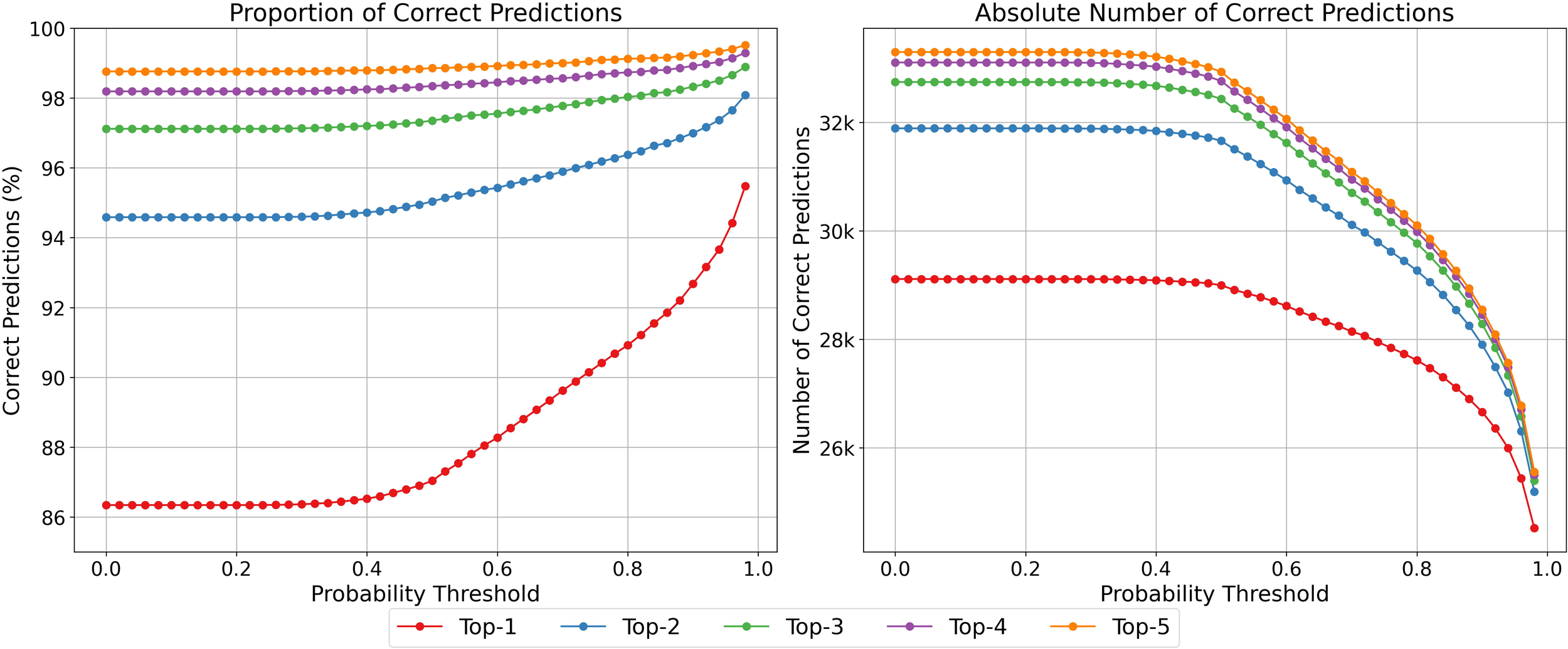
Progression of correct predictions across increasing probability thresholds. Left: Proportion of correct predictions. Right: Absolute number of correct predictions. Each curve corresponds to a different Top-k setting.
3.2 Per-class performance
3.2.1 Confusion matrix insights
Figures 5 and 6 show two versions of the normalized confusion matrix for the 95 phytoplankton classes, providing insight into per-class classification performance for the top-1 prediction.
Figure 5
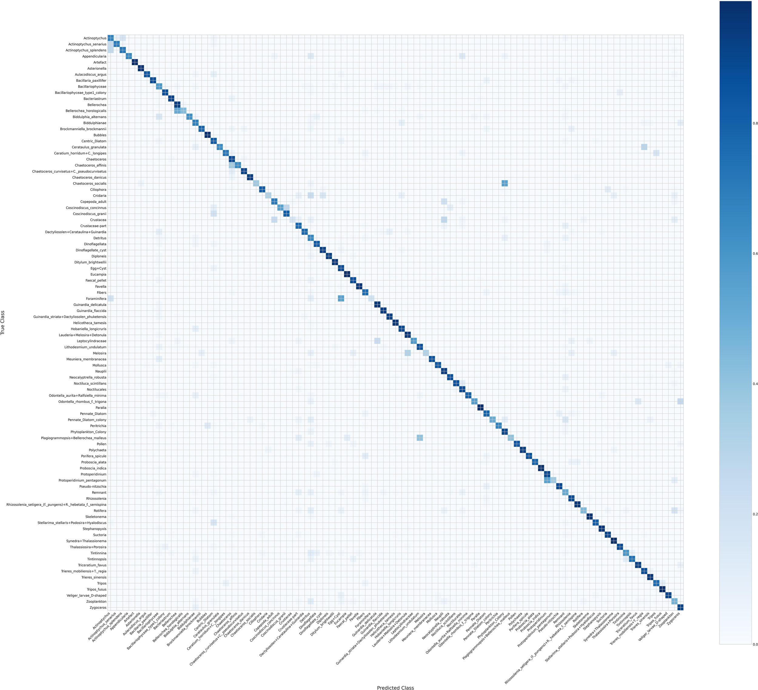
Confusion matrix of 95 phytoplankton classes.
Figure 6
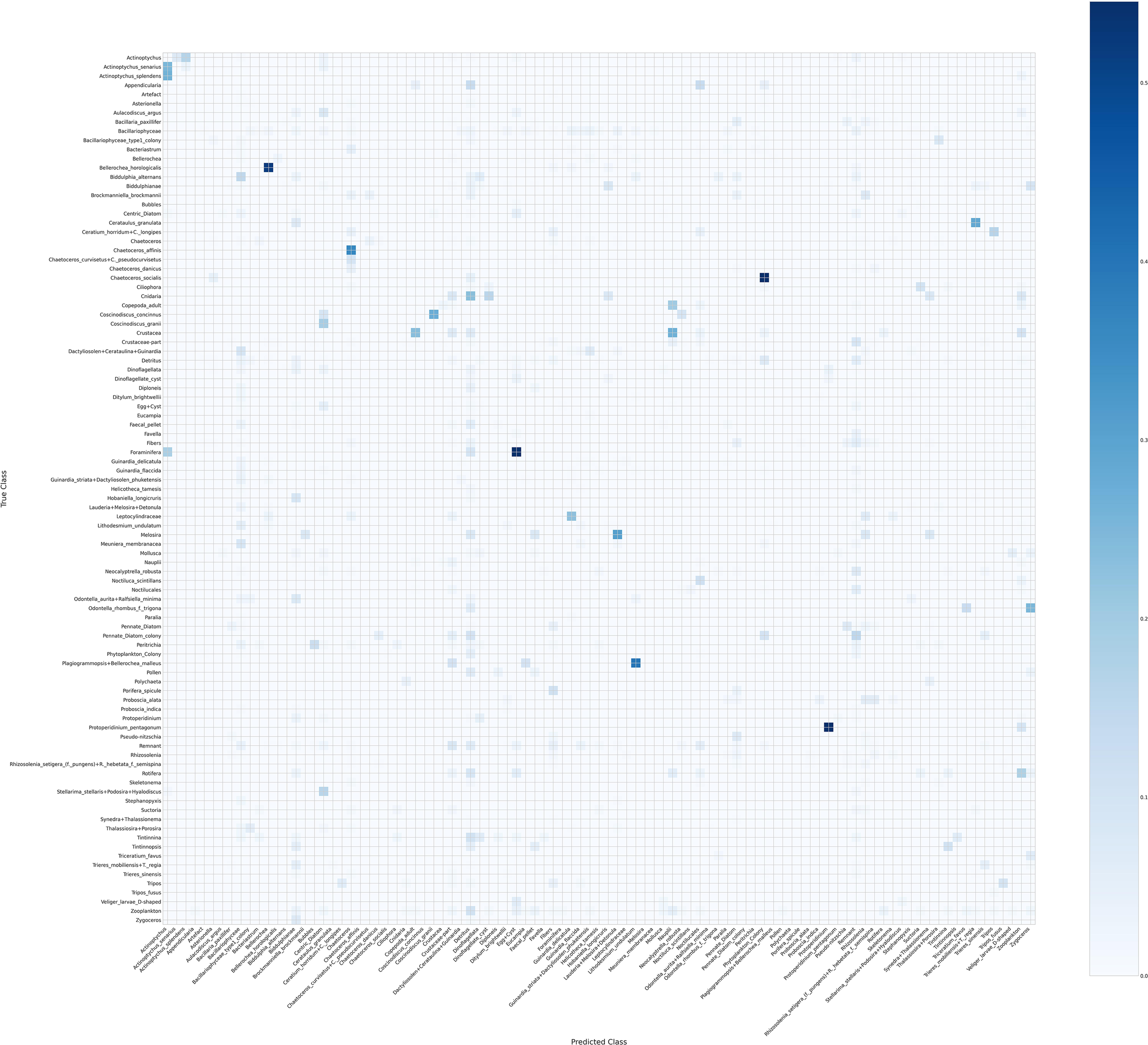
Confusion matrix of the 95 phytoplankton classes with the diagonal entries set to zero.
Figure 5 shows the standard confusion matrix, where diagonal dominance reflects that most predictions were correct. Off-diagonal entries highlight misclassifications, often between morphologically similar species or genera. For example, confusion is observed among species within the genera Actinoptychus and Chaetoceros, which is biologically plausible. Large and distinct taxa, such as Asterionella and bubbles, were classified with high accuracy. Misclassifications between Crustacea and Crustacea-part also appear plausible given their morphological similarities.
Figure 6 shows the same matrix but with diagonal entries set to zero to improve visual contrast and better highlight the misclassifications. Despite the diagonal being zeroed, a faint diagonal-like pattern remains, often corresponding to cases where the predicted genus is correct even if the species is not. Vertical lines in this matrix indicate that the model tends to over-predict certain classes, such as Detritus and Remnant, reflecting systematic biases in the predictions.
Overall, these matrices together provide a clear picture of both the strengths and limitations of the model, highlighting which classes are reliably predicted and where confusion occurs.
3.2.2 Class-specific metric summary
Table 4 summarizes the classification performance across various phytoplankton classes in terms of precision, recall, and F1-score. The results reveal considerable variation in per-class performance, reflecting the confusion patterns observed earlier. Several classes—such as Artefact, Asterionella, Bubbles, Chaetoceros danicus, Ditylum brightwellii, Eucampia, Helicotheca tamesis, the grouped taxa Lauderia–Melosira–Detonula, Paralia, Proboscia indica, Stephanopyxis, Synedra–Thalassionema, and Tripos fusus—are classified with consistently high performance.
Table 4
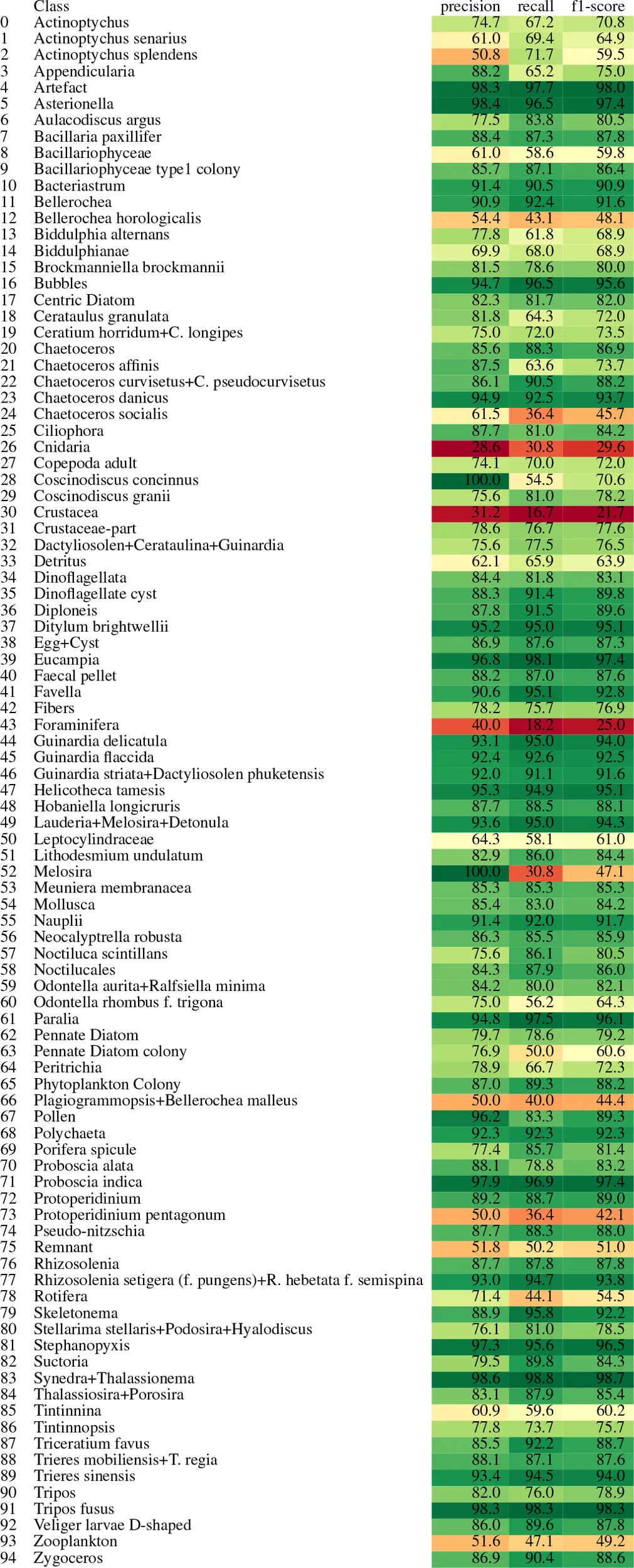
|
Class-wise performance metrics for the plankton classification model.
Each row corresponds to a taxonomic class. The table shows the precision, recall, and F1-score for each class. Cell background colors are used to visually highlight metric values, with greener shades indicating higher scores and yellower shades indicating lower scores. This color encoding helps to quickly identify well-performing versus underperforming classes.
In some of these cases, such as Coscinodiscus concinnus, Melosira, and Pollen, it is worth noting that the number of true positives is relatively low—6, 4, and 25 instances, respectively—all of which were correctly classified. This indicates perfect precision, with no false positives. However, the lower recall and F1 scores suggest that additional instances of these classes were missed by the model, pointing to the presence of false negatives.
Conversely, the model performs poorly on a few classes, most notably Cnidaria, Crustacea, and Foraminifera, where precision, recall, and F1-score are consistently low.
3.2.3 Probability threshold analysis per class
The model not only outputs the top five predicted classes for each image along with their associated confidence scores, but this section specifically analyzes the effect of applying different confidence thresholds on the top-1 predictions, broken down per class.
The results demonstrate that increasing the confidence threshold—i.e., filtering out top-1 predictions below a certain certainty level—generally improves the accuracy of the remaining predictions. However, this improvement comes at the cost of retaining fewer data points. Some illustrative examples are shown in Figure 7.
Figure 7
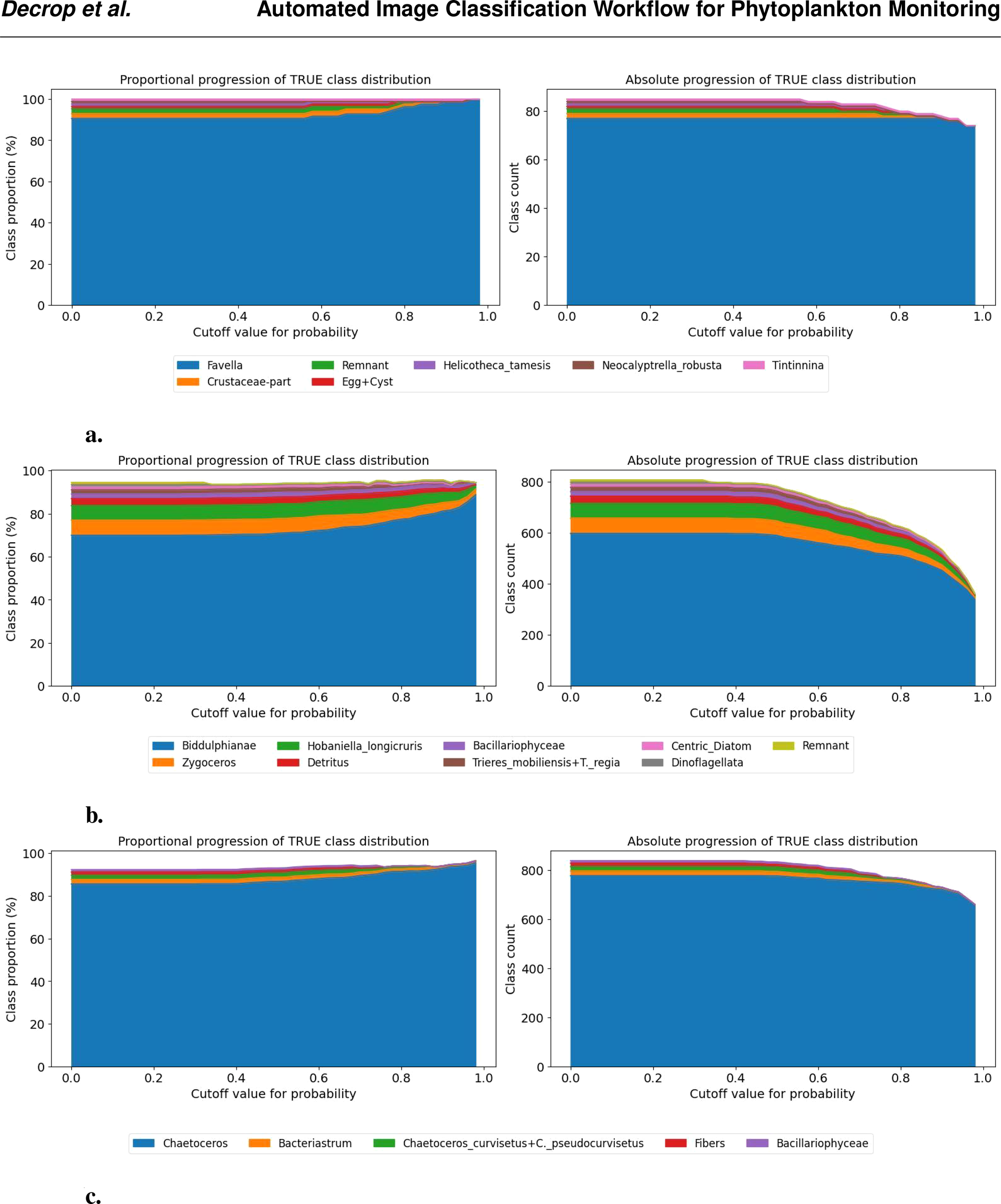
Class-wise progression of the true class distribution for different probability cutoff thresholds. The left panel shows the proportional representation (in %) of each true class among samples predicted as the given class, as the cutoff increases. The right panel shows the corresponding absolute counts. Only classes contributing more than 1% at any threshold are included. This visualization helps assess how class composition evolves as the classifier becomes more confident in its predictions. (A) Progression of Favella (B) Progression of Biddulphianae (C) Progression of Chaetoceros.
For instance, in the case of Favella (Figure 7a), increasing the threshold from 60% to 80% raises the correct-class proportion by 10% while retaining all true positives and filtering out misclassifications. As the threshold increases further, this trend continues. Around a 90% threshold, true positives begin to be filtered out, but the class purity reaches nearly 100% at a 98% threshold. In the examples of Biddulphianae and Chaetoceros (Figures 7b, c), a similar pattern is observed: increasing the cutoff improves the proportion of correct predictions, but some true positives are also lost. This effect is more pronounced in the case of Chaetoceros.
This thresholding approach enables the selection of a confidence level above which predictions can be reliably considered correct, potentially eliminating the need for manual verification. Conversely, for classes with lower model certainty, manual checks remain necessary for low-confidence predictions.
However, in some cases, the increase of cutoff does not correspond to higher performance, as illustrated in Figure 7. In the case of the Tripos fusus class (Figure 8a), performance remains stable and high regardless of the threshold, suggesting that no cutoff is needed. A similar situation occurs for the Asterionella class (Figure 8b), which consistently produces correct predictions after filtering out less than 1% misclassification. Additional examples of classes with near (e.g., Bubbles and Helicotheca tamesis) to very high (e.g., Proboscia indica and Stephanopyxis) accuracy can be found in the Supplementary Material (e.g., Bubbles and Helicotheca tamesis).
Figure 8
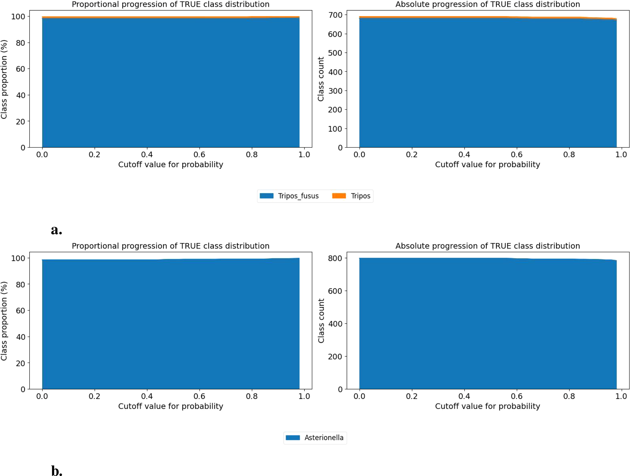
Class-wise progression of the true class distribution for different probability cutoff thresholds. The left panel shows the proportional representation (in %) of each true class among samples predicted as the given class, as the cutoff increases. The right panel shows the corresponding absolute counts. Only classes contributing more than 1% at any threshold are included. This visualization helps assess how class composition evolves as the classifier becomes more confident in its predictions. (A) Progression of Tripos fusus (B) Progression of Asterionella.
These class-specific threshold analyses support tailored post-processing strategies depending on the predicted class and its confidence distribution.
3.3 Benchmark results
3.3.1 External-to-local test
We retrained the published model from Kraft et al. (2022b) on our dataset to evaluate its performance under our imaging conditions and class distributions. After retraining, the model achieved an overall F1-score of 85.14%, slightly lower than the 86.25% obtained by our own model on the same dataset. While the difference is modest—less than 1%—it demonstrates that the external architecture can learn effectively from our data but still falls short of the performance reached by our tailored approach.
A detailed comparison of classification metrics is presented in Table 5. This table shows that our model outperforms SYKE in almost all key metrics, including Accuracy, Weighted Precision, Micro Precision, Weighted Recall, Micro Recall, and corresponding F1-scores. SYKE only slightly exceeds our model in Macro Precision and Macro F1, suggesting that it may perform marginally better on underrepresented classes. Overall, however, our model maintains stronger and more consistent performance across both common and rare classes.
Table 5
| Metric | EfficientNetV2-B0 | ResNet (SYKE) |
|---|---|---|
| Accuracy | 86.34 | 85.32 |
| Weighted Precision | 86.24 | 85.33 |
| Micro Precision | 86.34 | 85.32 |
| Macro Precision | 81.08 | 82.32 |
| Weighted Recall | 86.34 | 85.32 |
| Micro Recall | 86.34 | 85.32 |
| Macro Recall | 77.62 | 77.27 |
| Weighted F1 | 86.25 | 85.14 |
| Micro F1 | 86.34 | 85.32 |
| Macro F1 | 78.76 | 78.77 |
| Training Time (days) | 1.57 | 3.05 |
| Total Parameters | 7.33 M | 11.35 M |
Comparison between previous Top-1 performance and new classification results.
Best value per metric is highlighted in bold. Processing time (in days) and total parameters are also shown.
In addition to higher accuracy, our model is also substantially faster: it was trained in 1.57 days, compared to 3.05 days for the SYKE model, representing a reduction of approximately 50% in processing time. This speedup can be attributed to the more compact architecture of EfficientNetV2-B0, which has fewer parameters (7.33 M) compared to the ResNet-based SYKE model (11.35 M), resulting in reduced computational load per training iteration. This combination of improved accuracy and reduced processing time highlights the practical advantage of our approach for large-scale, high-throughput plankton classification.
Taken together, these results indicate that our model provides a balanced and efficient solution, achieving state-of-the-art performance while also being scalable and suitable for operational use. The consistent improvement across metrics and the marked reduction in computational time underscore the benefits of our architectural and training adjustments, particularly in capturing subtle inter-class differences under our specific imaging setup.µ
3.3.2 Local-to-external test
Similarly, we retrained our model on the Baltic Sea dataset (Kraft et al., 2022b) to assess how well it generalizes to external data after adaptation. Our model achieved an overall F1-score of 98.3%, exceeding the 95% F1-score reported by Kraft et al. (2022a). This shows that our architecture not only generalizes effectively but also delivers state-of-the-art performance without requiring dataset-specific tuning beyond retraining.
4 Discussion
These results indicate that the model is highly reliable in predicting the correct class within its top few guesses and performs especially well when broader prediction tolerance is allowed. The alignment between micro and weighted scores reflects the model’s robustness across the full dataset. The slightly lower macro scores suggest variability in performance among classes, especially those with fewer samples. The balance between precision and recall, as indicated by the F1 scores, confirms that the model maintains a good trade-off between identifying the correct classes and avoiding false positives. This supports the model’s suitability for practical applications, particularly in scenarios where identifying the top few likely classes is sufficient.
Figure 4 illustrates a key trade-off: increasing the probability threshold improves prediction certainty but reduces the number of samples considered. Including more candidate predictions (e.g., Top-2 or Top-3) improves the correct prediction rate while discarding fewer data points. This highlights a practical tuning parameter depending on the intended application—favoring either higher confidence or broader coverage.
Performance depends on both the frequency of classes in the dataset and how visually distinctive they are. This is a typical issue in imbalanced datasets, where trained classifiers often become biased toward the more prevalent classes Johnson and Khoshgoftaar (2019).
To quantify this effect, species were grouped into bins according to the number of samples, as summarized in Table 3. The table shows a clear trend: classification performance depends strongly on class frequency in the test set. Species with fewer than 50 samples exhibit lower Top-1 accuracy (67.7%), while those with 51–200 samples improve to 80.8%, and species with 201–800 samples reach 92.0%. Interestingly, the most abundant species (801–880 samples) show a slight drop in Top-1 accuracy to 85.3%, likely due to intra-class variability or label noise.
Top-3 accuracies further demonstrate the model’s robustness, with all bins exceeding 88% and the most abundant classes reaching 97.2%, indicating that the correct class is almost always among the top three predictions. Top-5 accuracies remain consistently high across all bins (more than 93%), confirming that even rare taxa are generally ranked among the top predictions.
This trend is reflected in specific examples: dominant and well-represented classes such as Artefact (880 samples), Asterionella (826 samples), and Eucampia (832 samples) achieve high performance, whereas underrepresented or morphologically diverse classes, including Cnidaria (13 samples), Crustacea (30 samples), and Foraminifera (11 samples), remain more challenging. These observations highlight the importance of considering class frequency when interpreting performance and reinforce the practical value of Top-K predictions and probability thresholds to balance precision and recall for underrepresented classes, particularly in semi-automated or expert-assisted labeling pipelines.
This underperformance is due to three factors. A first factor is due to methodological constraints, where certain taxa, such as Cnidaria, need alternative collection methods (e.g., plankton nets, vertical hauls, or larger-volume filtration) for sufficient representation. Increasing targeted sampling for these taxa could improve classification accuracy. A second factor is due to morphologically diverse, but rare taxa, such as Crustacea or Foraminifera. These groups are relatively rare and their morphology changes significantly when the angle of the imaged particle changes. Models need training for each of these angles to have representative output. And finally, meroplanktonic taxa, alike many zooplankton, change morphology throughout their life history, making it difficult for a model to recognize more than one life stage, and should be adjusted in the model. However – as flowcam is not designed to measure either of the above, the model excluded these particular cases to keep precision of targeted taxa high. For ecological applications, under-sampled taxa may be omitted or prioritized differently, allowing the model to focus on consistently sampled phytoplankton groups with strong reliability.
This pattern is also evident in borderline cases. For instance, Coscinodiscus concinnus, Pollen, and Melosira show high precision but lower recall due to low sample counts, illustrating how small class sizes can inflate apparent precision while masking recall limitations. These observations highlight the importance of dataset balance and class-specific morphology when interpreting performance and planning future data collection.
The challenges of class imbalance and taxonomic complexity suggest that model improvements—such as data augmentation, hierarchical classification, or targeted sampling—may benefit rare or difficult taxa. While no augmentations were applied in our experiments, a flexible augmentation pipeline is available in the accompanying GitHub notebooks, allowing future users to explore transformations such as flips, rotations, cropping, or color adjustments if needed. The strong performance at Top-3 and Top-5 levels aligns with practical workflows in marine ecology, where model predictions can assist expert taxonomists by presenting multiple likely taxa. This approach accelerates annotation while retaining human oversight. To further contextualize our results, we benchmarked our model against the publicly available Baltic Sea phytoplankton dataset (Kraft et al., 2022b). Both architectures were retrained on each other’s datasets to ensure a fair comparison. The published Kraft model achieved an F1-score of 85.14% on our dataset after retraining, demonstrating that their architecture can adapt to new imaging conditions, though slightly below the 86.25% obtained by our model. Conversely, our model achieved an F1-score of 98.3% on the Baltic Sea dataset, exceeding the 95% reported by Kraft et al. (2022a).
These findings indicate that while both architectures can generalize when retrained, our model exhibits stronger cross-dataset performance and maintains state-of-the-art accuracy across distinct phytoplankton imaging datasets. Beyond overall accuracy, our model also demonstrates consistent performance across both common and rare classes, as indicated by the combined metrics presented in Table 5. In contrast, the SYKE model, while slightly better in Macro metrics, shows reduced overall F1, highlighting that our approach better balances class-specific and global performance.
In addition, our model is significantly faster in training, processing the dataset twice as fast as the SYKE model. The combination of higher accuracy, more balanced class performance, and reduced computational time underscores the robustness and scalability of our approach.
Overall, these results suggest that our CNN-based architecture is not only capable of learning from diverse imaging conditions but also well-suited for operational plankton monitoring, where both accuracy and efficiency are critical. The performance consistency across datasets further reinforces the generalizability of our model, making it a strong candidate for deployment in automated plankton classification pipelines, long-term ecological monitoring, and cross-regional studies.
Integration of the classifier within the iMagine infrastructure further enhances its usability. The platform provides a modular marketplace where the classifier is available alongside complementary tools, including annotation software that can serve as an alternative to internal systems. Labelling tools and recommended workflows are discussed in detail in the iMagine best practices paper Azmi et al. (2025).
This setup promotes Open Science, standardized workflows, and scalable plankton image annotation. The model is accessible to any registered user for testing5 and can also be deployed in production via the OSCAR inference solution provided by the iMagine platform.
Some limitations remain. The current model relies on single-image input, which may be insufficient for taxa with subtle structural differences. Performance may also degrade on images from different optical sensor setups without domain adaptation.
Future work could focus on further mitigating current limitations. The successful retraining of our model on a different phytoplankton dataset demonstrates that transfer learning can effectively generalize to new imaging conditions, suggesting strong potential for broader application. Domain adaptation techniques could further enhance robustness when dealing with subtle differences in optical setups or sampling protocols. Additionally, while our study employed a pure CNN-based architecture (EfficientNetV2-B0), recent work demonstrates that transformer-based and hybrid models, such as Vision Transformers and Swin Transformers, can capture richer spatial–temporal features and may offer performance improvements, particularly for morphologically variable taxa (Kyathanahally et al., 2022; Maracani et al., 2023). Exploring these architectures in future research could help generalize automated plankton classification to even more diverse datasets and imaging conditions.
In conclusion, improved automated classification of phytoplankton images has important ecological implications, enabling faster processing of large datasets and more timely assessments of blooms or biodiversity shifts. While the introduction highlights speed, it is equally important to consider validation strategies. Not all outputs require the same level of validation: some classes (e.g., Tripos fusus) are consistently classified well, while others (e.g., Foraminifera) are more prone to misclassification. Adjusting the probability threshold, as illustrated in Figure 4, can filter out uncertain predictions and improve overall reliability.
Identifying priority classes for validation allows targeted efforts, focusing on challenging categories and reducing unnecessary verification for reliably classified groups. This approach is especially valuable when human validation is a limiting factor due to high data volume. Strategically allocating validation efforts optimizes resources, improves downstream analysis efficiency, and enhances the overall utility of automated classification within marine monitoring platforms.
Statements
Data availability statement
To support reproducibility, transparency, and further research—aligned with the FAIR principles (Wilkinson et al., 2016)—we provide open access to the full image library, the annotated training dataset, and the fully trained classifier model. The FlowCam image collection, containing segmented regions of interest (ROIs) from phytoplankton observations in the Belgian Part of the North Sea (BPNS), is available via the VLIZ Marine Data Archive (Flanders Marine Institute (VLIZ), 2024). The annotated subset used for training has been published on Zenodo LifeWatch observatory data: phytoplankton annotated training set by FlowCam imaging in the Belgian Part of the North Sea (Decrop et al., 2024), together with the final trained classifier (Decrop and Lagaisse, 2025). This accessibility enables other researchers to benchmark and improve upon the classification models, fostering collaboration and accelerating advances in plankton image analysis.
Author contributions
WD: Visualization, Conceptualization, Writing – review & editing, Project administration, Methodology, Writing – original draft. RL: Writing – original draft, Conceptualization, Project administration, Writing – review & editing, Data curation. JM: Writing – review & editing. CM: Writing – review & editing, Supervision, Resources. IH: Writing – review & editing, Software, Resources. AC: Writing – review & editing, Software, Resources. KD: Supervision, Writing – review & editing, Resources.
Funding
The author(s) declare that financial support was received for the research and/or publication of this article. This work has been funded by the European Union’s Horizon Europe research and innovation programme under grant number 101058625 as part of the iMagine project. It also made use of infrastructure provided by VLIZ, funded by the Research Foundation – Flanders (FWO; Grant I002021N) as part of the Belgian contribution to LifeWatch.
Acknowledgments
We extend our sincere gratitude to the iMagine project, funded by the European Union’s Horizon Europe research and innovation programme under grant number 101058625. We thank the project managers and all partners involved for their efforts in fostering the creation of open-access image repositories for AI-based image analysis services. This work was also supported by the Research Foundation - Flanders (FWO) under the framework of the Flemish contribution to LifeWatch, a landmark European Research Infrastructure on the European Strategy Forum on Research (ESFRI) roadmap. Finally, we are grateful to the VLIZ researchers and crew of the RV Simon Stevin for their practical support during the monthly sampling campaigns and to the Flemish Ministry of Mobility and Public Works (DAB VLOOT) for operating the vessel and facilitating the surveys.
Conflict of interest
The authors declare that the research was conducted in the absence of any commercial or financial relationships that could be construed as a potential conflict of interest.
Generative AI statement
The author(s) declare that Generative AI was used in the creation of this manuscript. Generative AI tools ChatGPT by OpenAI was used during the preparation of this manuscript for purposes such as language editing, improving clarity, and checking grammar. The authors reviewed and verified all AI-generated content to ensure its accuracy and appropriateness. No generative AI tools were used for data analysis, interpretation, or drawing scientific conclusions.
Any alternative text (alt text) provided alongside figures in this article has been generated by Frontiers with the support of artificial intelligence and reasonable efforts have been made to ensure accuracy, including review by the authors wherever possible. If you identify any issues, please contact us.
Publisher’s note
All claims expressed in this article are solely those of the authors and do not necessarily represent those of their affiliated organizations, or those of the publisher, the editors and the reviewers. Any product that may be evaluated in this article, or claim that may be made by its manufacturer, is not guaranteed or endorsed by the publisher.
Supplementary material
The Supplementary Material for this article can be found online at: https://www.frontiersin.org/articles/10.3389/fmars.2025.1699781/full#supplementary-material
Footnotes
1.^ https://dashboard.cloud.imagine-ai.eu/catalog/modules/phyto-plankton-classification.
2.^ https://ecotaxa.obs-vlfr.fr/.
3.^ https://dashboard.cloud.imagine-ai.eu/.
4.^ https://github.com/lifewatch/phyto-plankton-classification.
5.^ https://docs.ai4eosc.eu/en/latest/howtos/try/dashboard-gradio.html.
References
1
Azmi E. Alibabaei K. Kozlov V. Krijger T. Accarino G. Ayata S.-D. et al . (2025). Best practices for ai-based image analysis applications in aquatic sciences: The imagine case study. Ecol. Inf.91, 103306. doi: 10.1016/j.ecoinf.2025.103306
2
Benfield M. C. Grosjean P. Culverhouse P. F. Irigoien X. Sieracki M. E. Lopez-Urrutia A. et al . (2007). Rapid: research on automated plankton identification. Oceanography20, 172–187. doi: 10.5670/oceanog.2007.63
3
Blaschko M. B. Holness G. Mattar M. A. Lisin D. Utgoff P. E. Hanson A. R. et al . (2005). “ Automatic in situ identification of plankton,” in 2005 Seventh IEEE Workshops on Applications of Computer Vision (WACV/MOTION’05), vol. 1. (Piscataway, New Jersey, USA: IEEE), 79–86.
4
Chollet F. et al . (2015). Keras. Available online at: https://keras.io (Accessed March 2025).
5
Decrop W. Lagaisse R. (2025). Pre-trained phytoplankton species classifier model. Immonen: Master’s thesis, Lappeenranta, Finland: LUT University. doi: 10.5281/zenodo.15269453
6
Decrop W. Lagaisse R. Jonas M. Muyle J. Amadei Martínez L. Deneudt K. (2024). Lifewatch observatory data: phytoplankton annotated trainingset by flowcam imaging in the belgian part of the north sea (version v1). Immonen: Master’s thesis, Lappeenranta, Finland: LUT University. doi: 10.5281/zenodo.10554845
7
Deng J. Dong W. Socher R. Li L.-J. Li K. Fei-Fei L. (2009). “ Imagenet: A large-scale hierarchical image database,” in 2009 IEEE conference on computer vision and pattern recognition ( Ieee), 248–255.
8
De Vargas C. Audic S. Henry N. Decelle J. Mahé F. Logares R. et al . (2015). Eukaryotic plankton diversity in the sunlit ocean. Science348, 1261605. doi: 10.1126/science.1261605
9
Dubelaar G. B. Gerritzen P. L. Beeker A. E. Jonker R. R. Tangen K. (1999). Design and first results of cytobuoy: A wireless flow cytometer for in situ analysis of marine and fresh waters. Cytometry: J. Int. Soc. Analytical Cytology37, 247–254. doi: 10.1002/(SICI)1097-0320(19991201)37:4<247::AID-CYTO1>3.0.CO;2-9
10
Ducklow H. W. Steinberg D. K. Buesseler K. O. (2001). Upper ocean carbon export and the biological pump. Oceanography14, 50–58. doi: 10.5670/oceanog.2001.06
11
Dunker S. Boho D. Wäldchen J. Mäder P. (2018). Combining high-throughput imaging flow cytometry and deep learning for efficient species and life-cycle stage identification of phytoplankton. BMC Ecol.18, 51. doi: 10.1186/s12898-018-0209-5
12
Eerola T. Batrakhanov D. Barazandeh N. V. Kraft K. Haraguchi L. Lensu L. et al . (2024). Survey of automatic plankton image recognition: challenges, existing solutions and future perspectives. Artif. Intell. Rev.57, 114. doi: 10.1007/s10462-024-10745-y
13
European Commission . (1999). Implementation of Council Directive 91/271/EEC of 21 May 1991 concerning urban waste water treatment, as amended by Commission Directive 98/15/EC of 27 February 1998 : summary of the measures implemented by the member states and assessment of the information received pursuant to Articles 17 and 13 of the directive. Office for Official Publications of the European Communities ; Bernan Associates [distributor].
14
Faillettaz R. Picheral M. Luo J. Y. Guigand C. Cowen R. K. Irisson J.-O. (2016). Imperfect automatic image classification successfully describes plankton distribution patterns. Methods Oceanography15, 60–77. doi: 10.1016/j.mio.2016.04.003
15
Flanders Marine Institute (VLIZ) (2024). Lifewatch observatory data: phytoplankton observations by flowcam imaging in the belgian part of the north sea. Immonen: Master’s thesis, Lappeenranta, Finland: LUT University. doi: 10.14284/650
16
Garcíıa Á.L. (2019). Deepaas api: A rest api for machine learning and deep learning models. J. Open Source Software4, 1517. doi: 10.21105/joss.01517
17
Guo B. Nyman L. Nayak A. R. Milmore D. McFarland M. Twardowski M. S. et al . (2021). Automated plankton classification from holographic imagery with deep convolutional neural networks. Limnology Oceanography: Methods19, 21–36. doi: 10.1002/lom3.10402
18
Hays G. C. Richardson A. J. Robinson C. (2005). Climate change and marine plankton. Trends Ecol. Evol.20, 337–344. doi: 10.1016/j.tree.2005.03.004
19
Henrichs D. W. Anglès S. Gaonkar C. C. Campbell L. (2021). Application of a convolutional neural network to improve automated early warning of harmful algal blooms. Environ. Sci. pollut. Res.28, 28544–28555. doi: 10.1007/s11356-021-12471-2
20
Immonen V. (2025). Cross-modal learning for plankton recognition.
21
Irisson J.-O. Salinas L. Colin S. Picheral M. (2022). Ecotaxa: a tool to support the taxonomic classification of large datasets through supervised machine learning. In. SFEcologie2022.
22
Johnson J. M. Khoshgoftaar T. M. (2019). Survey on deep learning with class imbalance. J. big Data6, 1–54. doi: 10.1186/s40537-019-0192-5
23
Keçeli A. S. Kaya A. Keçeli S. U. (2017). Classification of radiolarian images with hand-crafted and deep features. Comput. Geosciences109, 67–74. doi: 10.1016/j.cageo.2017.08.011
24
Kerr T. Clark J. R. Fileman E. S. Widdicombe C. E. Pugeault N. (2020). Collaborative deep learning models to handle class imbalance in flowcam plankton imagery. IEEE Access8, 170013–170032. doi: 10.1109/ACCESS.2020.3022242
25
Kraft K. Velhonoja O. Eerola T. Suikkanen S. Tamminen T. Haraguchi L. et al . (2022a). Towards operational phytoplankton recognition with automated high-throughput imaging, near-real-time data processing, and convolutional neural networks. Front. Mar. Sci.9, 867695. doi: 10.3389/fmars.2022.867695
26
Kraft K. Velhonoja O. Seppälä J. Hällfors H. Suikkanen S. Ylöstalo P. et al . (2022b). SYKE-plankton IFCB 2022. doi: 10.23728/B2SHARE
27
Krizhevsky A. Sutskever I. Hinton G. E. (2012). Imagenet classification with deep convolutional neural networks. Adv. Neural Inf. Process. Syst.25, 84–90. doi: 10.1145/3065386
28
Kyathanahally S. P. Hardeman T. Reyes M. Merz E. Bulas T. Brun P. et al . (2022). Ensembles of data-efficient vision transformers as a new paradigm for automated classification in ecology. Sci. Rep.12, 18590. doi: 10.1038/s41598-022-21910-0
29
Lagaisse R. (2024). Lifewatch Belgium: Flowcam sampling and lab protocol for imaging microphytoplankton in the belgian part of the north sea ( Flanders Marine Institute). Available online at: https://www.protocols.io/view/lifewatch-Belgium-flowcam-sampling-and-lab-protoco-6qpvr8e6zlmk/v1.
30
Lagaisse R. Dillen N. Bakeev D. Decrop W. Focke P. Mortelmans J. et al . (2025). Advancing long-term phytoplankton biodiversity assessment in the north sea using an imaging approach (London, UK: Manuscript submitted for review to *Scientific Data*).
31
LeCun Y. Bengio Y. Hinton G. (2015). Deep learning. nature521, 436–444. doi: 10.1038/nature14539
32
Lumini A. Nanni L. (2019). Deep learning and transfer learning features for plankton classification. Ecol. Inf.51, 33–43. doi: 10.1016/j.ecoinf.2019.02.007
33
Luo J. Y. Irisson J.-O. Graham B. Guigand C. Sarafraz A. Mader C. et al . (2018). Automated plankton image analysis using convolutional neural networks. Limnology Oceanography: Methods16, 814–827. doi: 10.1002/lom3.10285
34
Maracani A. Pastore V. P. Natale L. Rosasco L. Odone F. (2023). In-domain versus out-of-domain transfer learning in plankton image classification. Sci. Rep.13, 10443. doi: 10.1038/s41598-023-37627-7
35
MinIO (2020). Minio, a leader in high performance object storage, launches the minio subscription network globally. Comput. Technol. J.274. Available online at: https://www.businesswire.com/news/home/20200818005060/en/.
36
Ollevier A. Mortelmans J. Vandegehuchte M. B. Develter R. De Troch M. Deneudt K. (2022). A video plankton recorder user guide: Lessons learned from in situ plankton imaging in shallow and turbid coastal waters in the belgian part of the north sea. J. Sea Res.188, 102257. doi: 10.1016/j.seares.2022.102257
37
Orenstein E. C. Beijbom O. (2017). “ Transfer learning and deep feature extraction for planktonic image data sets,” in 2017 IEEE Winter Conference on Applications of Computer Vision (WACV) ( IEEE), 1082–1088.
38
Pedraza A. Bueno G. Deniz O. Ruiz-Santaquiteria J. Sanchez C. Blanco S. et al . (2018). “ Lights and pitfalls of convolutional neural networks for diatom identification,” in optics, photonics, and digital technologies for imaging applications V, vol. 10679. ( SPIE), 88–96.
39
Pérez A. Risco S. Naranjo D. M. Caballer M. Moltó G. (2019). “ On-premises serverless computing for event-driven data processing applications,” in 2019 IEEE 12th International Conference on Cloud Computing (CLOUD), Piscataway, New Jersey, USA: IEEE (Institute of Electrical and Electronics Engineers)414–421. doi: 10.1109/CLOUD.2019.00073
40
Picheral M. Guidi L. Stemmann L. Karl D. M. Iddaoud G. Gorsky G. (2010). The underwater vision profiler 5: An advanced instrument for high spatial resolution studies of particle size spectra and zooplankton. Limnology Oceanography: Methods8, 462–473. doi: 10.4319/lom.2010.8.462
41
Pierella Karlusich J. J. Ibarbalz F. M. Bowler C. (2020). Phytoplankton in the tara ocean. Annu. Rev. Mar. Sci.12, 233–265. doi: 10.1146/annurev-marine-010419-010706
42
Sieracki C. K. Sieracki M. E. Yentsch C. S. (1998). An imaging-in-flow system for automated analysis of marine microplankton. Mar. Ecol. Prog. Ser.168, 285–296. doi: 10.3354/meps168285
43
Soh Y. Song J. Hae Y. (2018). Multiple plankton detection and recognition in microscopic images with homogeneous clumping and heterogeneous interspersion. J. Institute Convergence Signal Process.19, 35–41. doi: 10.23087/jkicsp.2018.19.2.001
44
Sosa-Trejo D. Bandera A. González M. Hernández-León S. (2023). Vision-based techniques for automatic marine plankton classification. Artif. Intell. Rev.56, 12853–12884. doi: 10.1007/s10462-023-10456-w
45
Sosik H. M. Olson R. J. (2007). Automated taxonomic classification of phytoplankton sampled with imaging-in-flow cytometry. Limnology Oceanography: Methods5, 204–216. doi: 10.4319/lom.2007.5.204
46
Sournia A. Chrdtiennot-Dinet M.-J. Ricard M. (1991). Marine phytoplankton: how many species in the world ocean? J. Plankton Res.13, 1093–1099. doi: 10.1093/plankt/13.5.1093
47
Tan M. Le Q. (2021). “ Efficientnetv2: Smaller models and faster training,” in International conference on machine learning. 10096–10106 (Sweden: PMLR).
48
Tett P. Carreira C. Mills D. K. van Leeuwen S. Foden J. Bresnan E. et al . (2008). Use of a Phytoplankton Community Index to assess the health of coastal waters. – ICES. J Mar Sci. 65:1475–1482. doi: 10.1093/icesjms/fsn161
49
Thai-Nghe N. Gantner Z. Schmidt-Thieme L. (2010). “ Cost-sensitive learning methods for imbalanced data,” in The 2010 International joint conference on neural networks (IJCNN). 1–8 (Barcelona, Spain: IEEE).
50
Wilkinson M. D. Dumontier M. Aalbersberg I. J. Appleton G. Axton M. Baak A. et al . (2016). The fair guiding principles for scientific data management and stewardship. Sci. Data3. doi: 10.1038/sdata.2016.18
51
Winder M. Sommer U. (2012). Phytoplankton response to a changing climate. Hydrobiologia698, 5–16. doi: 10.1007/s10750-012-1149-2
52
Zheng H. Wang R. Yu Z. Wang N. Gu Z. Zheng B. (2017). Automatic plankton image classification combining multiple view features via multiple kernel learning. BMC Bioinf.18, 570. doi: 10.1186/s12859-017-1954-8
Summary
Keywords
convolutional neural network, phytoplankton, image classification, FlowCAM, BPNS, biodiversity monitoring
Citation
Decrop W, Lagaisse R, Mortelmans J, Muñiz C, Heredia I, Calatrava A and Deneudt K (2025) Automated image classification workflow for phytoplankton monitoring. Front. Mar. Sci. 12:1699781. doi: 10.3389/fmars.2025.1699781
Received
05 September 2025
Revised
29 October 2025
Accepted
24 November 2025
Published
15 December 2025
Volume
12 - 2025
Edited by
Jin Zhou, Tsinghua University, China
Reviewed by
Šimon Bilík, VŠB-Technical University of Ostrava, Czechia
Rajmohan Pardeshi, Chandigarh Group of Colleges Jhanjeri, India
Updates
Copyright
© 2025 Decrop, Lagaisse, Mortelmans, Muñiz, Heredia, Calatrava and Deneudt.
This is an open-access article distributed under the terms of the Creative Commons Attribution License (CC BY). The use, distribution or reproduction in other forums is permitted, provided the original author(s) and the copyright owner(s) are credited and that the original publication in this journal is cited, in accordance with accepted academic practice. No use, distribution or reproduction is permitted which does not comply with these terms.
*Correspondence: Wout Decrop, wout.decrop@vliz.be
Disclaimer
All claims expressed in this article are solely those of the authors and do not necessarily represent those of their affiliated organizations, or those of the publisher, the editors and the reviewers. Any product that may be evaluated in this article or claim that may be made by its manufacturer is not guaranteed or endorsed by the publisher.