Abstract
Assessing the spatial distribution of ichthyoplankton populations is crucial for understanding marine ecosystems. However, identifying the factors that influence their abundance and distribution presents a significant challenge, where seasonal change plays an essential role in the environmental variables. In this study, we analyzed abiotic and biotic factors from the eastern Arabian Sea during the early summer monsoon to characterize ichthyoplankton assemblages and examine the impact of physical processes and environmental variables on their spatial abundance and distribution. Although the eastern Arabian Sea (EAS) is one of the most productive fishing areas in the Indian Ocean, information on ichthyoplankton in this region has been limited. Our findings reveal a heterogeneous distribution of ichtyoplankton across the EAS, which was significantly influenced by the upwelling-driven productive environment characterizing the EAS. Statistical analyses, including Generalized Additive Models (GAMs) and Principal Component Analysis (PCA), indicated a strong positive correlation between nutrient levels, chlorophyll-a concentrations, and zooplankton biomass with the abundance of fish eggs and larvae. Conversely, sea surface temperature and salinity were found to have negative relationship with ichthyoplankton abundance and distribution. These findings provide valuable insights into the ecology of ichthyoplankton within a major eastern boundary upwelling ecosystem highlighting the impact of physical processes and varying environmental drivers on ichthyoplankton populations in a productive marine environment.
1 Introduction
Studies on factors influencing the spatial distribution and abundance of ichthyoplankton have increased in recent years, mainly because these studies are crucial for understanding the stock replenishment process and the future productivity of fish stocks (Höffle et al., 2018; Yang et al., 2021). Addressing the challenges related to the early life stages of pelagic fish species can be quite complex due to their variability in distribution. Furthermore, different species have different life cycles and reproductive behaviours and respond uniquely to environmental changes. Finally, our understanding of the mechanisms that determine the suitability of specific habitats for spawning remains limited (Lima et al., 2022; Lowerre-Barbieri et al., 2011). Additionally, the physical processes inherent in the marine ecosystem play a crucial role in modulating reproductive site selection, interacting with the specific preference and responses of fish species (Tiedemann et al., 2017). Consequently, identifying areas critical for early developmental stages becomes increasingly complex and necessitates considerations of multiple interacting factors within the marine ecosystem.
Ichthyoplankton, which includes fish eggs and larvae, serve as valuable indicators for identifying spawning and nursery areas respectively, as well as understanding population replenishment patterns in marine ecosystems. Due to their high susceptibility to predation and mortality - especially when there are mismatches between the timing of fish stock renewal and plankton production (Kripa et al., 2018)- regular monitoring of these early developmental stages is essential for the development of effective fishery resource management policies (Fletcher et al., 2010; Van der Lingen and Huggett, 2003).
The eastern Arabian Sea (EAS), located in the tropical Indian Ocean, is one of the world’s major eastern boundary upwelling ecosystems and is recognized as one of the most productive regions globally (Kumar et al., 2000; Gupta et al., 2016). The biological productivity of the EAS is strongly influenced by the monsoonal wind reversal and associated changes in hydrography, which in turn affect fish behavior, seasonality, distribution, and abundance in this ecosystem (Banse, 1987; McCreary et al., 1996, McCreary et al., 2009; Wiggert et al., 2005, 2006; Shankar et al., 2019). During the summer monsoon, wind-driven upwelling is crucial for sustaining the region’s high productivity (Kusum et al., 2014). This upwelling begins near the southern tip of the west coast around late May and gradually moves northward (Smitha et al., 2008). In contrast, during the winter monsoon, productivity is enhanced by winter cooling and convective overturning (Kumar and Prasad, 1996). As a result, primary productivity and phytoplankton biomass in the EAS exhibit clear seasonality, peaking during both the southwest (summer) monsoon and the northeast (winter) monsoon (Marra and Barber, 2005; Reddy et al., 2024).
The summer monsoon is typically regarded as the most productive period in the EAS, making fisheries during this time critically important (Shankar et al., 2019; Kumar et al., 2000). This period is also considered critical for the replenishment of fish populations through early life stages; however, information regarding the spatial abundance and distribution of ichthyoplankton, along with location-specific spawning periods in this region, remains largely unknown (Rathnasuriya et al., 2021). This lack of information presents a significant challenge for policymakers, particularly in determining appropriate trawl ban periods in specific locations to protect juvenile fish and support sustainable fisheries management (Abdussamad et al., 2013; Ciannelli et al., 2014; Filho et al., 2020; Mohamed et al., 2014).
To address this gap, a comprehensive study was conducted along the EAS during the early summer monsoon (ESM) period. This study aimed to examine the spatial distribution and abundance of ichthyoplankton in the EAS and assess the impact of environmental variables and physical processes on the variability influencing the distribution and abundance patterns. By understanding these factors, this research provides crucial insights into the ecological dynamics of fish population renewal driven by early life stages, contributing to the development of effective fisheries management strategies.
2 Materials and methods
2.1 Study area
An ichthyoplankton survey was undertaken on-board CRV Sagar Tara under the Fisheries Resources and Habitat Assessment (FRHA) program of the Centre for Marine Living Resources and Ecology (CMLRE), Ministry of Earth Sciences (MoES), India. The study was carried out in the eastern Arabian Sea (EAS) spanning a wide geographical area from 8°N to 20°N covering 14 transects, with each transect separated by 1° latitude and depths ranging from 10 to 1000 m (Figure 1). Sampling was done during the early summer monsoon period (ESM) (23rd May, 2023 – 21th June, 2023) and a total of 72 sampling locations were covered. In the present study, to obtain spatially distinct information, the study region EAS was divided into three distinct zones, South Zone (SZ), Central Zone (CZ) and North Zone (NZ), based on physicochemical attributes. The south zone extended from Tuticorin to Calicut (8° - 11°N), the central zone from Kannur to Ratnagiri (12° - 17° N) and the north zone extended from Dapoli to northwards (18° - 20° N). A total of 72 sampling locations were investigated during the study.
Figure 1
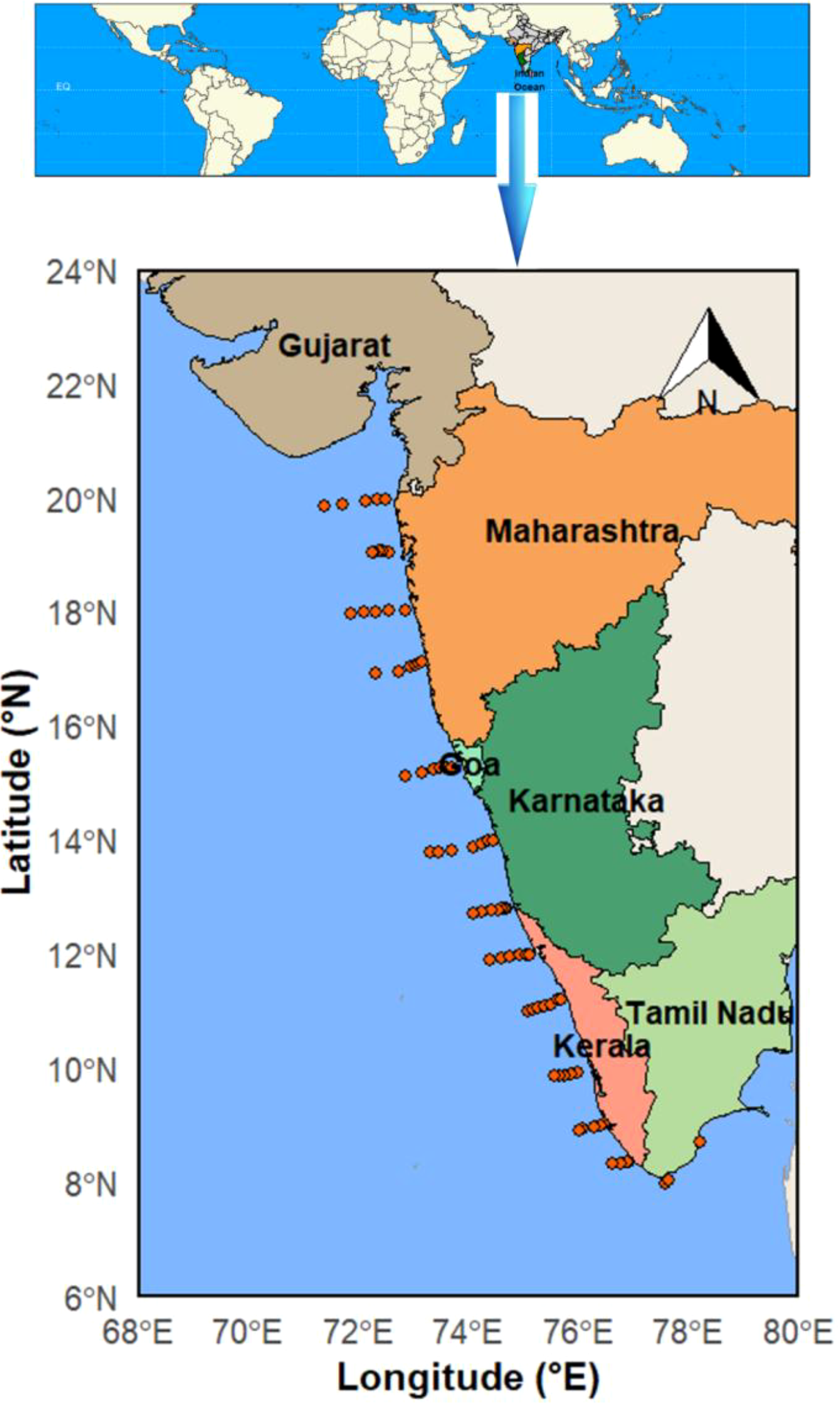
The distribution of sampling locations in the eastern Arabian Sea.
2.2 Estimation of abiotic variables
Meteorological and oceanographic parameters during the study were also investigated along with the ichthyoplankton sampling. The environmental factors, sea surface temperature (SST), sea surface salinity (SSS), dissolved oxygen (DO), phosphate, silicate, nitrite, nitrate, and chlorophyll-a (Chl-a) were simultaneously measured at each sampling station. Wind speed during the study period was obtained from the Automatic Weather Station on board the research vessel. Oceanographic parameters (SST and SSS) were collected from each station using an SBE Sea-Bird thermosalinograph with an accuracy of temperature ± 0.001°C, conductivity ± 0.0003 S/m. The thermosalinograph continuously measured the surface water samples (3–4 m depth) along the ship track.
A Hydrobios Niskin water sampler was used at every sampling location to collect surface water samples for dissolved oxygen (DO) and dissolved inorganic nutrients. For the estimation of DO, from Niskin sampler, 60 ml water sample was taken in DO bottles and was fixed by adding 0.5 ml each of Winkler reagents, and titrated against 0.001N Hypo using a Dosimat (Metrohm, Switzerland) following standard procedures (Grasshoff, 1983). Surface water samples were collected using a Niskin sampler to estimate the dissolved inorganic nutrients. Nutrients (nitrite, phosphate, and silicate) were estimated following the standard colourimetric techniques (Grasshoff, 1983) using a segmented flow autoanalyzer (SKALAR SAN++). Nitrate was also analyzed using an autoanalyzer but following the method of García-Robledo et al. (2014). The analytical precision, expressed as standard deviation based on replicate analyses, was ± 0.005, 0.027, 0.009, and 0.037 μM for NO2−, NO3−, PO4−, and SiO4−, respectively.
2.3 Estimation of biotic variables
As a proxy of phytoplankton biomass, Chlorophyll a was estimated and for that purpose, 2L water samples were collected from a depth of 3–4 m using a Niskin sampler. The size-fractioned chlorophyll a in each sampling location was analyzed by sequentially filtering water samples. Initially, the samples were passed through a 200-μm and 20-μm mesh filter to categorize the meso and micro fraction respectively. Immediately after filtration, the meshes were reverse -washed with distilled water and passed through glass fibre filters (GF/F; nominal pore size 0.7 μm) to determine the Chlorophyll a pigment concentration corresponding to the respective size classes. Following this, the filtered water samples were passed through 2-μm and 0.2-μm polycarbonate filters to estimate the nanoplankton and picoplankton biomass, respectively. The pigments of each size class were extracted using a 90% acetone and analyzed using a UV/Vis Shimadzu spectrophotometer following the protocol of Strickland and Parsons (1972). The total chlorophyll a was calculated by summing the chlorophyll a concentrations from all the size-fractionated phytoplankton groups.
Zooplankton samples were collected from every sampling location, ranging from coastal areas with a depth of 10 m to offshore locations at depth of 1000 m. This was done by surface (at 1m depth) hauling of a ring net for mesozooplankton (mesh size 300 µm, with a mouth area 0.44 m2) for 10 minutes. A hauling speed of 3 knots per hour was maintained to reduce zooplankton avoidance of the net. A calibrated flow meter (Hydro-Bios, Model 438110) was attached to the mouth of the net to estimate the volume of water filtered by the net. The biomass of the zooplankton samples was estimated by the displacement volume method and was expressed as ml m−3 (Harris et al., 2000). Immediately after the collection of zooplankton samples, the ichthyoplankton (fish eggs and fish larvae) were sorted separately from the mesozooplankton samples under a stereo-zoom microscope (Leica M80). The abundance of both fish eggs and larvae was expressed as individuals per 100 cubic meters (ind/100 m3). All the samples were preserved in 95% ethanol solution for the detailed taxonomic analysis.
2.4 Statistical analysis
The statistical analysis was selected to ensure the study provided a robust understanding of the complex ecological relationships in the EAS. Firstly, ANOVA (with two-tailed P values and 95% confidence intervals) was carried out to rigorously validate the study’s spatial partitioning by testing whether the means or medians of biotic and abiotic variables differed significantly between the predefined geographical zones. Before the analysis, the datasets were assessed for normality in their distribution using the D’ Agostino and Pearson omnibus normality test. Based on the results of the normality test, parametric ANOVA was applied to the variables exhibiting a Gaussian distribution. Conversely, a non-parametric test (Kruskal Wallis test) was used for variables with a non-Gaussian distribution. All analyses were performed using GraphPad Prism version 5.00 for Windows, GraphPad Software, San Diego, California, USA (www.graphpad.com).
Additionally, to explore the relationship between the abundance of fish eggs and larvae and the abiotic variables sea surface temperature (SST), sea surface salinity (SSS), wind speed, nutrients, and dissolved oxygen (DO) as well as other biotic variables (chlorophyll a and zooplankton biomass), principal component analysis (PCA) was conducted based on fourth root transformed data using the statistical program PAST version 2.02 (Hammer et al., 2001). PCA served as an exploratory tool to reduce data dimensionality and identify key environmental gradients influencing ichthyoplankton variability and thus helped to identify the preferred spawning environment for fishes in the EAS during the early summer monsoon (ESM).
The constrained canonical analysis of principal coordinates (CAP) is crucial for constrained hypothesis testing (Anderson and Willis, 2003), and hence the analysis was carried out to assess the distinctness and similarities of sampling transects in the EAS, focusing on the controlling variables affecting ichthyoplankton abundance. For the CAP analysis, the abiotic variables included SST, SSS, wind speed, nutrients, and DO, while the biotic variables comprised chlorophyll a and zooplankton biomass. This analysis utilized the similarity metric of Euclidean distance, and fourth root transformed data were used employing PRIMER (Clark and Warwick, 2001).
Finally, a Generalized Additive Model (GAM) was specifically chosen to model the non-linear, non-monotonic ecological responses of ichthyoplankton (fish eggs and larvae) abundances and their environment, including chlorophyll-a (chl-a) concentration and zooplankton biomass, which linear models cannot capture effectively. For this model, both fish egg and larval abundances were specified as response variables, while chl-a, zooplankton biomass and all environmental variables were incorporated as predictor variables. The GAM was fitted using a Gamma family with a default log-link function. Additionally, the latitude of the sampling locations was incorporated as a covariate for the analysis. The statistical significance of predictor variables was assessed using p-values, where a p-value < 0.05 indicated a significant relationship between the predictor and response variables. The performance of the GAM was evaluated using the AIC value and deviance explained, where a low AIC and a high deviance indicate a better model fit. All GAM analyses were conducted using the mgcv package in RStudio (version 4.4.3).
3 Results
3.1 Physicochemical environment and identified physical process
During the ESM, SST was found to range from 25.6°C to 32°C (Mean [M] ± standard deviation [SD], 30.4 ± 1.5°C) with a prominent spatial variation in distribution from south to north (Figure 2a). SST was relatively low in the south zone (up to 11°N) (M ± SD, 29.0 ± 1.9°C). Thereafter, in the central and northern zones, SST showed less spatial variation (Supplementary Table 1a). However, the northernmost transect also exhibited relatively low SST during this period (Figure 2a). The result of the statistical analysis exhibited significant differences in SST distribution among the north, central and southern EAS [ANOVA: F(2,71)=24.87, P<0.001], while in the case of pairwise Tukey’s multiple comparison post hoc test, the southern EAS showed significant variation with northern and central EAS (Supplementary Table 2a). The propagation of the low SST from the southern part towards the north indicated the occurrence and progression of coastal upwelling in this region, and this signature of upwelling was evident up to 11°N.
Figure 2
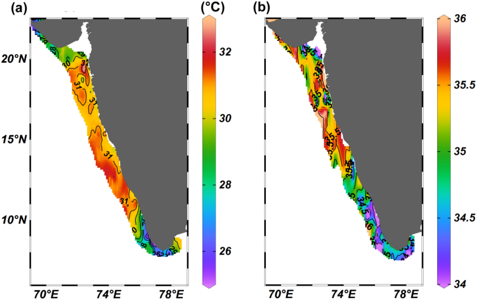
The distribution of (a) sea surface temperature (b) sea surface salinity in the eastern Arabian Sea.
The SSS in the study region ranged from 33.6 to 35.6 (M ± SD, 35.0 ± 0.4), with a north-south gradient in distribution along spatial scale (Figure 2b). SSS was high in the northern and central part, compared to the southern EAS (M ± SD, 34.5 ± 0.4) and the spatial variation was statistically significant [ANOVA: F (2,71) =58.85, P<0.001]. During the study period, the region experienced wind speed from 0.8 to 11.1 (m/s) (Supplementary Figure 1). Relatively high wind speed was recorded at the southern EAS and at the northern tips of the EAS, though the difference was not statistically significant [ANOVA: F(2,71) = 2.913, P = 0.061]. In pairwise Tukey’s multiple comparison post hoc test, significant variation in wind speed was not observed between regions (Supplementary Table 2c).
3.2 Chemical environments
During the study, the dissolved inorganic nitrite (NO2) concentration varied from 0.01 to 0.33 μM with a mean of 0.05 ± 0.05 μM. The southern part of EAS exhibited relatively high nitrite levels M ± SD, 0.1 ± 0.1 μM) compared to the northern and central part (Figure 3a, Supplementary Table 1b) with a significant difference among these three regions [ANOVA: F(2,71)=32.92, P < 0.001]. In the case of pairwise Tukey’s multiple comparison post hoc test, the variation was significant between the central and southern regions only (Supplementary Table 2d). The dissolved inorganic nitrate concentration (NO3) in the study area varied from 0.01 to 1.9 μM (M ± SD, 0.3 ± 0.4 μM) (Figure 3b). Spatially, the southern part (M ± SD, 0.5 ± 0.5 μM), where upwelled water was observed, exhibited relatively higher NO3 concentration than the north and central EAS (Figure 3b, Supplementary Table 1b) and the variation was found to be statistically significant [ANOVA: F(2,71)=7.052, P = 0.002]. In the case of the pairwise Tukey’s multiple comparison post hoc test, the central zone was distinctly different in nitrate concentration from the north and southern parts of the EAS (Supplementary Table 2e). The dissolved inorganic silicate levels in the study area (SiO3) ranged from 0.94 to 10.9 μM (M ± SD, 3.3 ± 2.1μM) (Figure 3c). The central and northern EAS was characterized by relatively high silicate concentration compared to the southern part of the EAS (Figure 3c). However, the variation among the three zones [Kruskal-Wallis statistics H (2,71) = 3.52, P = 0.172] and also the pairwise Tukey’s multiple comparison post hoc test exhibited insignificant variation (Supplementary Table 2f). Dissolved oxygen (DO) ranged from 166 to 250 μM (M ± SD, 205 ± 25 μM) in the study region with a significant difference among the three regions [ANOVA: F (2,71) =29.42, P < 0.001] (Figure 4) while in the case of the pairwise Tukey’s multiple comparison post hoc test, the southern part exhibited significant variation with both the northern and central region of EAS (Supplementary Table 2g).
Figure 3
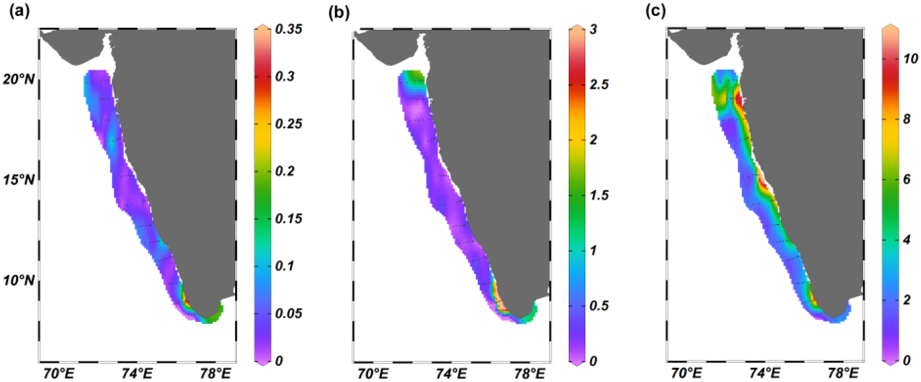
The distribution of (a) nitrite (µM) (b) nitrate (µM), and (c) silicate (µM) in the eastern Arabian Sea.
Figure 4
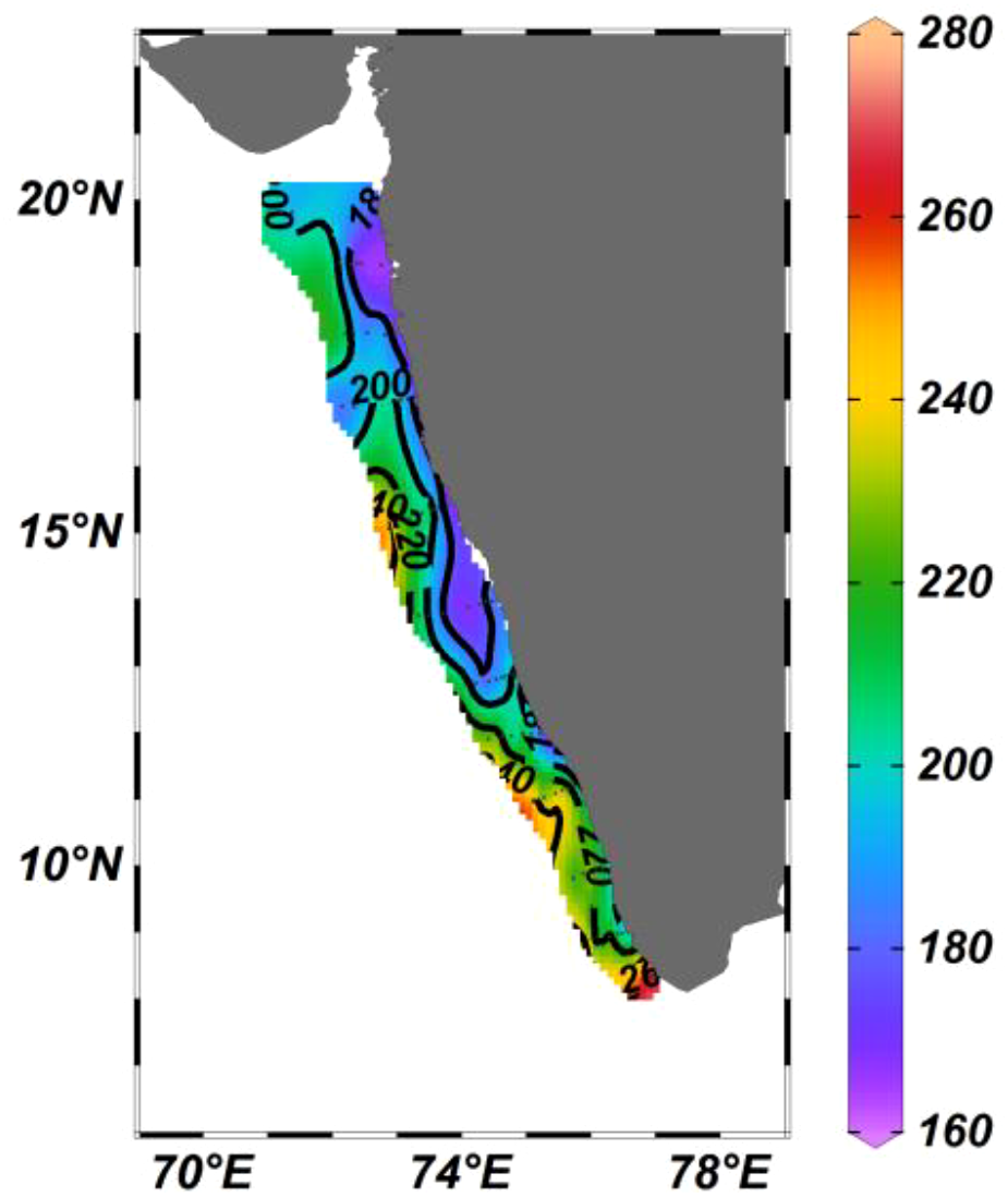
The distribution of dissolved oxygen (μM) in the eastern Arabian Sea.
3.3 Biotic environment
3.3.1 Chlorophyll-a and zooplankton biomass
The chl-a ranged from 0.03 to 6.07 mg/m3 (M ± SD, 0.5 ± 1.0 mg/m3) (Figure 5a) during ESM (study period). It was relatively high in the coastal locations compared to offshore locations (Figure 5a). Spatially, during ESM, chl-a, was relatively high in the southern part of EAS (M ± SD, 0.7 ± 1.2 mg/m3) characterized by upwelled water as compared to the northern (M ± SD, 0.3 ± 0.3 mg/m3) and central part (M ± SD, 0.4 ± 0.9 mg/m3) (Figure 5a, Supplementary Table 1b) with a statistically significant difference [Kruskal-Wallis statistics H (2,71) = 7.057, P = 0.029]. However, in the case of pairwise Dunn’s multiple comparison post hoc test, no significant variation was observed (Supplementary Table 2h).
Figure 5
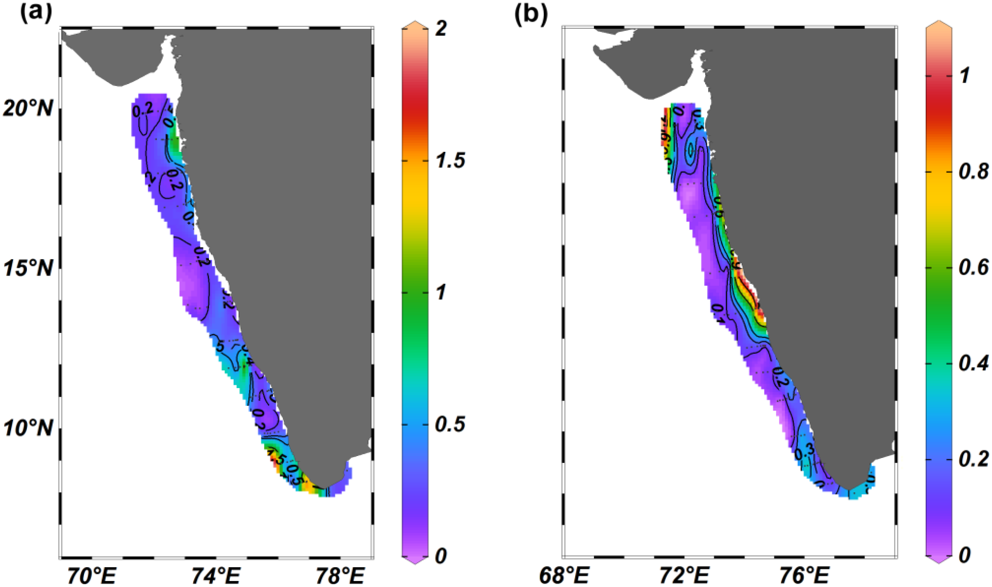
The distribution of (a) Chlorophyll a (mg/m3), and (b) zooplankton biomass (ml/m3) in the eastern Arabian Sea.
Meanwhile, the zooplankton biomass in the study region varied from 0.01 to 1.09 ml/m3 (M ± SD, 0.2 ± 0.2 ml/m3) (Figure 5b). Relatively high values were observed in a few coastal sampling locations, especially in the central region. Along with a few offshore locations in the northern EAS, moderate zooplankton standing stock was observed in the entire southern EAS, where the presence of upwelled water was evident (Figure 5b, Supplementary Table 1b). However, the variation in the zooplankton biomass among the three regions of EAS was statistically insignificant in [Kruskal-Wallis statistics H (2,71) = 0.4836, P = 0.785]. The result of the pairwise Dunn’s multiple comparison post hoc test also did not show any significant variation between any two regions (Supplementary Table 2i).
3.3.2 Icthyoplankton abundance and distribution
3.3.2.1 Fish egg abundance and distribution
During the ESM, the abundance of fish eggs ranged between 0 and 41182 ind/100m3 with a mean abundance of 1127 ± 5566 ind/100m3. Although fish eggs were observed along all the transects, their abundance was markedly high in the southern part (M ± SD, 2180 ± 8422 ind/100m3) compared to the north (M ± SD, 10 ± 31 ind/100m3) and central EAS (M ± SD, 868 ± 4034 ind/100m3) (Figure 6a, Supplementary Table 1b). The results of the one-way ANOVA of fish egg abundance among the three regions also exhibited significant difference [Kruskal-Wallis statistics H (2,71)= 22.52, P <0.001]. Similarly, the pairwise Dunn’s multiple comparison post hoc test among the regions also showed significant variation between all of them (Supplementary Table 2j).
Figure 6
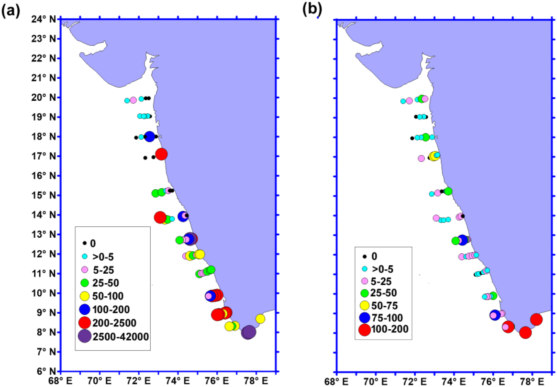
The distribution of (a) fish egg (ind/100m3), and (b) fish larvae (ind/100m3) in the eastern Arabian Sea.
3.3.2.2 Fish larval abundance and distribution
Fish larval abundance was several-fold lower compared to fish egg abundance and ranged between 0 and 192 ind/100 m3 with a mean abundance of 19 ± 34 ind/100 m3 (Figure 6b). Although, fish larval abundance was relatively high in the southern EAS (M ± SD, 31 ± 50 ind/100m3) than central (M ± SD, 15 ± 21 ind/100m3) and northern EAS M ± SD, 8 ± 15 ind/100m3), the variation was not statistically significant (ANOVA: F(2,71)=2.568, P = 0.084).
3.4 Data analyses
3.4.1 Principal component analysis
The results of the PCA biplot exhibited the interrelation existing between the abundance of fish eggs and larvae and the significant ecological variables (biotic and abiotic) during the ESM (Figure 7). The first two axes described 44% of the variance. During ESM, fish egg and fish larvae abundance were positively correlated with chl-a, nitrite, nitrate and zooplankton biomass, and their abundances were higher in the SZ. In contrast, they were negatively correlated with SST and SSS (Figure 7).
Figure 7
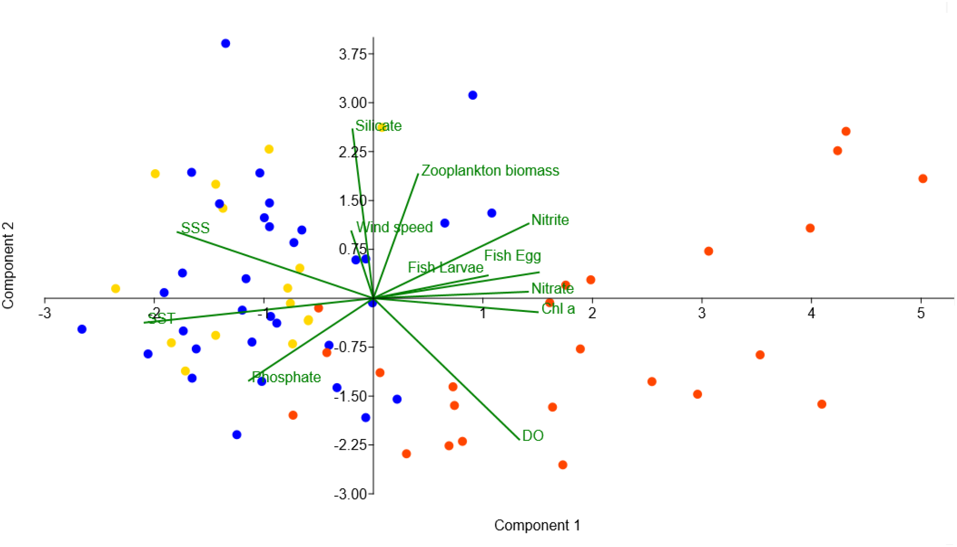
PCA biplot showing the interrelationships of the abundance of the ichthyoplankton and different abiotic and biotic variables in the eastern Arabian Sea during early summer monsoon (Gold, Blue and Orange colored dots indicate sampling locations of north, central and south zone, respectively).
3.4.2 Canonical analysis of principal coordinates (CAP)
The CAP analysis done based on the distribution of all the controlling variables (both abiotic and biotic) in the sampling locations showed that along the axis of the CAP, the position of the sampling locations of the southern transects was distinct from the central and northern transects (Figure 8) with a squared canonical correlation value (δ2) of 0.7364 indicating a discrete environment in the southern EAS from the northern and central transects.
Figure 8
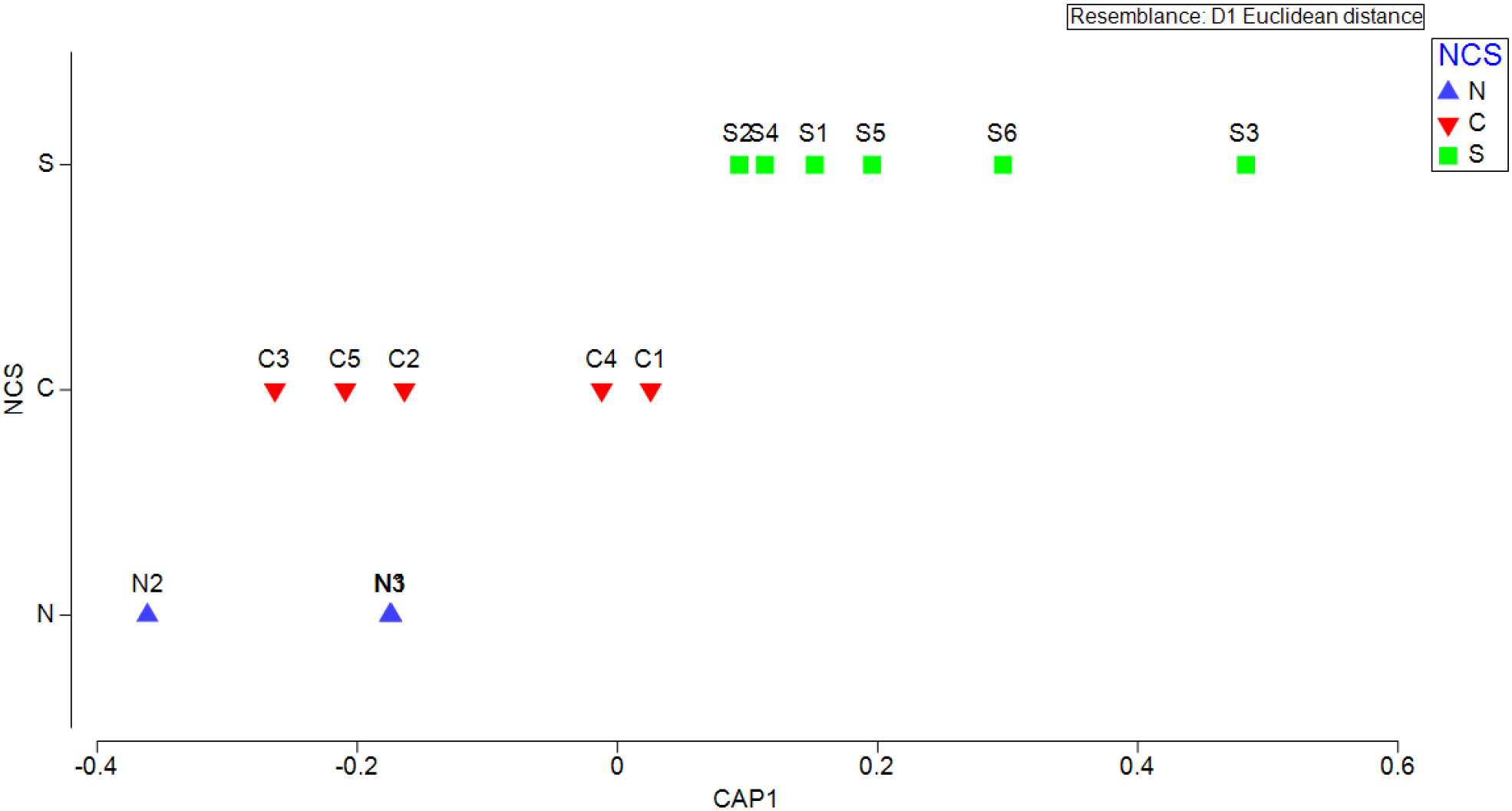
Canonical analysis of principal coordinates (CAP) based on the distribution of controlling variables (SST, SSS, wind speed, nutrients, DO, chlorophyll a and zooplankton biomass) along sampling transects in the eastern Arabian Sea during early summer monsoon period (N: North, C: Central, S: South).
3.4.3 GAMs for fish egg and larvae abundance in the EAS
GAMs were developed to assess the influence of environmental variables on the abundance and distribution of ichthyoplankton in the EAS. The models employed a Gamma family with a log-link function, selecting significant variables based on p-values and deviance explained (Table 1).
Table 1
| (a) | ||||||||||
|---|---|---|---|---|---|---|---|---|---|---|
| Parametric coefficients: | ||||||||||
| Term | Estimate | Std. Error | t-value | p-value | Significance | |||||
| Intercept | 2.8301 | 0.1405 | 20.14 | <2e-16 | *** | |||||
| Approximate Significance of Smooth Terms: | ||||||||||
| Term | edf | Ref.df | F | p-value | Significance | |||||
| s(Latitude) | 4.494 | 5.440 | 12.002 | 1.47e-06 | *** | |||||
| s(WindSpeed) | 2.439 | 3.023 | 13.961 | 2.76e-06 | *** | |||||
| s(SST) | 1.000 | 1.000 | 14.339 | 0.000544 | *** | |||||
| s(Chl_a) | 8.716 | 8.944 | 9.141 | 5.90e-07 | *** | |||||
| s(SSS) | 3.924 | 4.712 | 6.325 | 0.000334 | *** | |||||
| s(DO) | 1.000 | 1.000 | 1.941 | 0.171876 | ||||||
| s(ZooplanktonBiomass) | 4.785 | 5.657 | 1.170 | 0.234782 | ||||||
| s(Silicate) | 1.000 | 1.000 | 2.336 | 0.134901 | ||||||
| s(Nitrite) | 1.000 | 1.000 | 8.332 | 0.006467 | ** | |||||
| s(Nitrate) | 2.294 | 2.843 | 5.471 | 0.003338 | ** | |||||
| s(Phosphate) | 3.764 | 4.544 | 3.924 | 0.011298 | ||||||
| Signif. codes: 0 ‘***’ 0.001 ‘**’ 0.01 ‘*’ 0.05 ‘.’ 0.1 ‘ ‘ 1 | ||||||||||
| R-sq.(adj) = 0.606 Deviance explained = 89.4% | ||||||||||
| GCV = 3.8653 Scale est. = 1.4219 n = 72 | ||||||||||
| AIC: 632.2251 | ||||||||||
| (b) | ||||||||||
|---|---|---|---|---|---|---|---|---|---|---|
| Parametric coefficients: Backward selected procedure | ||||||||||
| Term | Estimate | Std. Error | t-value | p-value | Significance | |||||
| Intercept | 2.0778 | 0.1429 | 14.54 | <2e-16 | *** | |||||
| Approximate Significance of Smooth Terms | ||||||||||
| Term | edf | Ref.df | F | p-value | Significance | |||||
| s(Latitude) | 1.000 | 1.000 | 18.704 | 6.35e-05 | *** | |||||
| s(Wind speed) | 7.509 | 8.415 | 4.316 | 0.000463 | *** | |||||
| s(SST) | 3.850 | 4.738 | 7.409 | 3.34e-05 | ** | |||||
| s(SSS) | 1.000 | 1.000 | 10.508 | 0.002004 | ** | |||||
| s(DO) | 1.000 | 1.000 | 7.495 | 0.008276 | ** | |||||
| s(Nitrate) | 1.000 | 1.000 | 11.284 | 0.001412 | ** | |||||
| Signif. codes: 0 ‘***’ 0.001 ‘**’ 0.01 ‘*’ 0.05 ‘.’ 0.1 ‘ ‘ 1 | ||||||||||
| R-sq.(adj) = 0.088 Deviance explained = 45% | ||||||||||
| GCV = 3.5123 Scale est. = 1.4706 n = 72 | ||||||||||
| AIC: 462.4409 | ||||||||||
Step-wise construction of a generalized additive model (GAM) to identify factors influencing the abundance and distribution of fish eggs (a) and larvae (b) in the Eastern Arabian Sea during the early summer monsoon (backward-selection procedure applied for fish larvae).
GAMs for fish egg and fish larvae abundance retained eleven environmental variables, including SST, SSS, Chl-a, nitrite, nitrate, silicate, phosphate, DO, wind speed, zooplankton biomass, and latitude as a covariate. The model for fish egg abundance explained 89.4% of the variance, while the model for fish larvae abundance explained 45%. The parametric coefficients for the intercept in both models were highly significant (P < 2e-16, each) (Tables 1a, b).
For fish eggs, latitude exhibited a statistically significant nonlinear effect (P = 1.47e-06), while wind speed (P = 2.76e-06), SST (P = 0.000544), chl-a (P = 5.90e-07), SSS (P = 0.000334), nitrite (P = 0.006467), nitrate (P = 0.003338) and phosphate (P = 0.011298) showed strong influences (Table 1a; Figure 9a). In comparison, the model for fish larvae indicated that latitude (P = 5.58e-05) and wind speed (P = 0.000213) were the strongest drivers, showing highly significant effects. SST (P = 0.002235), SSS (P = 0.001116), DO (P = 0.002414), and nitrate (P = 0.009182) also contributed significantly (Table 1b; Figure 9b). The Q-Q plot helped to check if the deviance residuals from the model followed a standard normal distribution, which is an ideal condition for GLMs when the model is correctly specified. It was found that in the case of the model for fish egg, the residuals are approximately normally distributed, whereas in the case of the fish larvae, they likely have slightly heavier tails than a pure normal distribution (Figure 10).
Figure 9
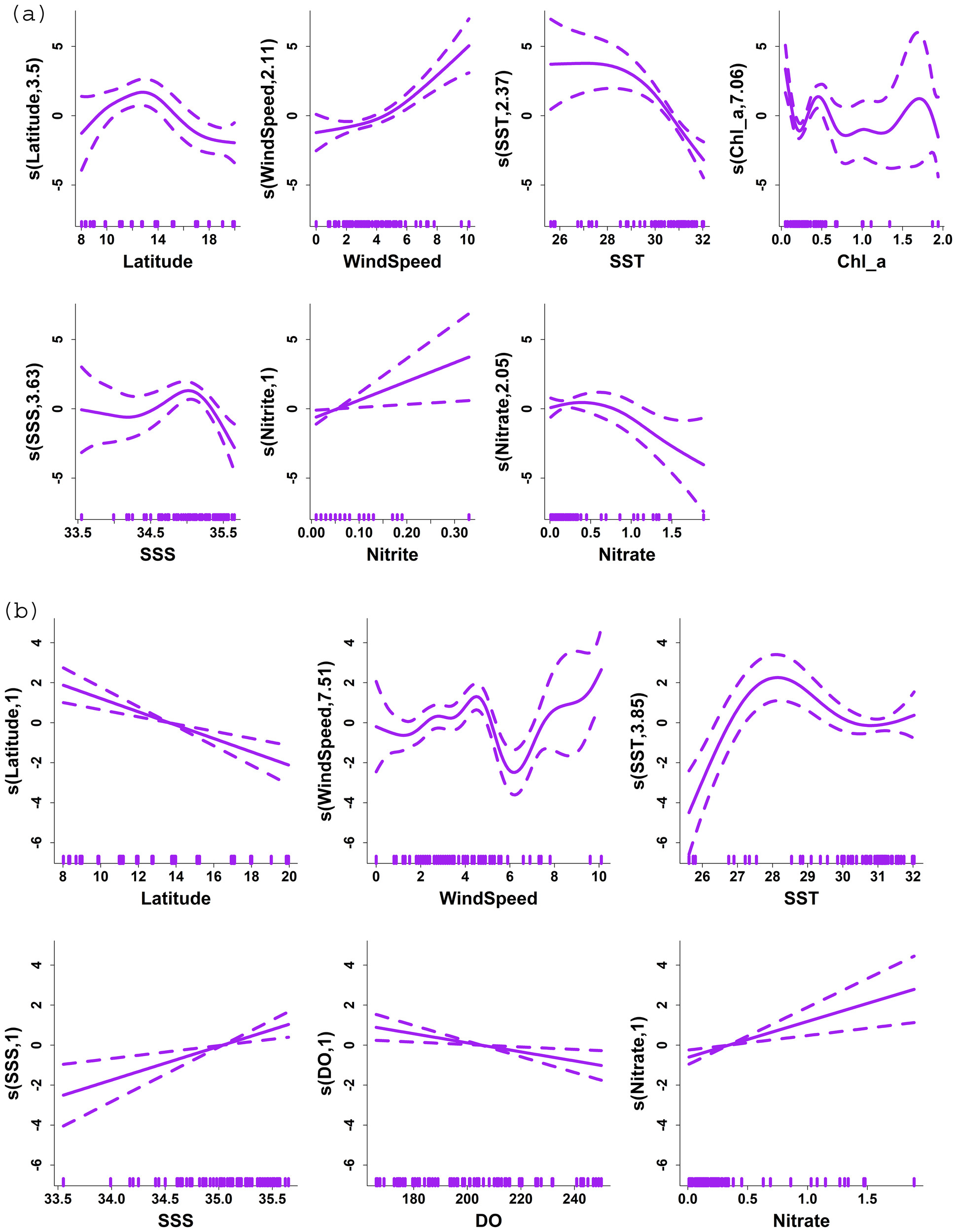
The partial plot illustrates the influence of environmental variables on the abundance of (a) fish eggs and (b) larvae modelled using a Generalized Additive Model (GAM) with a Gamma distribution and a log link function. The variables include sea surface temperature (SST), sea surface salinity (SSS), chlorophyll-a (Chl-a), nitrite, nitrate, silicate, phosphate, dissolved oxygen (DO), wind speed, zooplankton biomass, and latitude. Solid lines represent the smoothed effects, while dotted lines indicate the 95% confidence intervals.
Figure 10
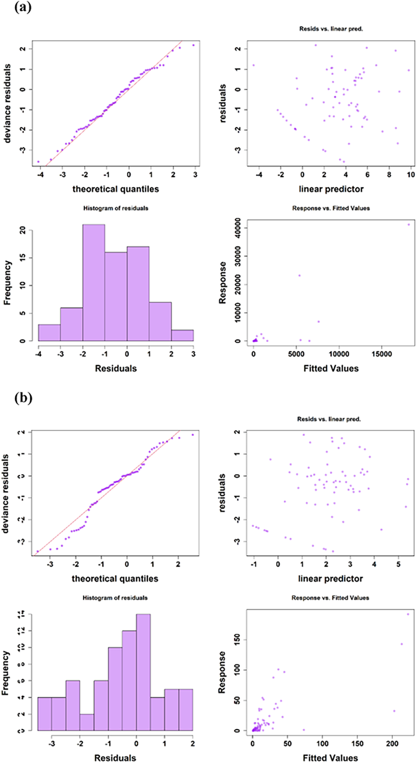
Diagnostic plots for assessing assumptions of the GAM model for (a) Fish eggs, and (b) Fish larvae.
4 Discussion
Environmental variables significantly influence the abundance and distribution of ichthyoplankton. Therefore, understanding the spatiotemporal distributions of ichthyoplankton and their responses to these environmental factors is crucial for developing effective management strategies (Cowen et al., 1993; Santos et al., 2017). The findings of this study provide insights into the variability in the abundance and distribution of ichthyoplankton during early summer monsoons in the EAS and identify the key factors affecting them during this period. The notably higher abundance of fish eggs in the southern part of EAS suggests a greater occurrence of fish spawning in this region during ESM.
While the summer monsoon is generally considered the most productive period in the EAS, leading to increased productivity and subsequent fish catches (Shankar et al., 2019; Kumar et al., 2000), the observed differences in the ichthyoplankton distribution during this study indicate that the ecological drivers do not uniformly influence fish stock replenishment throughout the EAS. The asymmetry in the controlling variables and physical processes likely contributes to the variation in fish spawning behaviour across the region, which is reflected in the differences in ichthyoplankton abundance observed among the southern, central, and northern parts of EAS.
In marine ecosystems, the variability in ichthyoplankton abundance is typically influenced by physical processes operating within the ecosystem and physicochemical variables (Tiedemann et al., 2017; Shankar et al., 2019). To understand the hydrographic environment of the EAS during the ESM, these physical processes, characterized by specific physicochemical conditions, were analyzed first. The heterogeneity observed in sea surface temperature (SST) not only reveals the uneven distribution of SST in the EAS but also helps to clarify the active physical processes in the system. Coastal waters marked by low SST in the southern EAS indicate an upwelling process in this region (Figure 2a).
With the onset of the summer monsoon during May, the upwelling is first observed at the southern tip of the west coast of India, and it propagates northward as the monsoon progresses (Smitha et al., 2008). Hence, the northward propagation of the upwelled water up to 11°N noted in this study aligns with the active upwelling process in this region during the ESM. Significant spatial variation in SST distribution among the northern, central and southern EAS (P<0.001) can be attributed to the surfacing of cool, subsurface waters due to the upwelling phenomenon in the southern EAS. However, the northernmost transect (20°N) also showed relatively low SST during the study period, potentially due to enhanced wind-driven mixing that brought cooler subsurface waters to the surface.
Regarding surface salinity, the spatial heterogeneity was less pronounced than that of SST, but it was still expected that the southern part of the EAS would have relatively lower surface salinity (SSS) compared to the north. Here, the exchange of low-salinity Bay of Bengal water with the EAS helps to maintain the observed north-south gradient. Although this gradient is most pronounced in winter due to the intrusion of Bay of Bengal water controlled by the coastal current in the southern region (Prasanna Kumar et al., 2004; Karati et al., 2018), a tendency for lower SSS in the south persists throughout the year with smaller spatial differences. However, the upwelling of high-salinity subsurface water in the southern ESA is expected to result in higher SSS in coastal waters than offshore waters (Reddy et al., 2024). This anticipated trend in SSS distribution was observed except along 10°N, where the fluvial inputs from seven rivers flowing through the Cochin estuary contribute to lowering the SSS of the coastal waters.
In terms of nutrients, the southern EAS exhibited higher concentrations, except for silicate, primarily due to upwelling, which brings nutrient-rich subsurface waters to the surface (Reddy et al., 2024; Gupta et al., 2016). This phenomenon resulted in elevated levels of nitrate and nitrite in the southern EAS, with significant differences noted between the southern and central regions, further indicating the influence of upwelling on nutrient distribution. Silicate distribution, however, was largely influenced by riverine input, with major rivers in the northern EAS, such as the Narmada and Tapti, contributing to higher silicate levels in the coastal waters.
Environmental factors, including physicochemical conditions, play a critical role in determining fish spawning areas and the spatial distribution of ichthyoplankton in marine ecosystems (Laprise and Pepin, 1995; Kingsford, 1993). The study revealed a higher phytoplankton standing stock in the southern part of EAS compared to the northern and central parts, driven by coastal upwelling processes active in this region. Upwelling-induced nutrient enrichment, coupled with elevated chlorophyll-a concentrations, is a characteristic feature of eastern boundary upwelling systems globally (Morales et al., 1996; Rueda-Roa and Muller-Karger, 2013; Vinayachandran et al., 2021). The moderate zooplankton biomass observed in the southern EAS indicates that the phytoplankton-rich environment supported this zooplankton population. Although high zooplankton biomass was recorded at specific coastal and offshore sites in the northern and central EAS, the consistently moderate levels in the south underscore the sustained influence of coastal upwelling in supporting zooplankton production.
Similar to the distribution patterns of phytoplankton and zooplankton, ichthyoplankton abundance also exhibited significant variation across the three zones of the EAS. The notably high abundance of fish eggs and larvae in the southern EAS likely coincided with the elevated plankton productivity in the region. The influence of upwelling was more pronounced in the southern EAS, particularly south of 11°N. This upwelling-driven, nutrient-enriched environment promoted enhanced primary and secondary production, providing the necessary food resources for the survival and development of the early life stages of fish. Such a food-rich habitat likely serves as a favourable spawning and nursery ground for various fish species. However, anthropogenic factors such as the high density of boats and ships and excessive fishing operations in coastal regions may negatively impact the presence of adult fish during their reproductive phase, potentially resulting in reduced spawning activity and lower egg abundance (Chermahini et al., 2021). Although these aspects were not assessed in our study, they might also have contributed to the heterogeneity of the ichthyoplankton distribution in the study region. Although species-level identification of ichthyoplankton was not carried out in the present study, the composition of adult fish landings along the west coast of India (Supplementary Table 3) was used as a proxy to infer the most likely egg and larval assemblages. In Kerala, the southernmost state along EAS, fish landing is dominated by oil sardine, anchovies and threadfin breams (CMFRI, 2023, 2024, and 2025), and hence there is a possibility of the contribution of these groups of fishes in the high abundance of ichthyoplankton in this region.
The PCA biplot demonstrating a positive association between ichthyoplankton abundance and several environmental variables, including chlorophyll-a concentration, nitrite and nitrate levels, as well as zooplankton biomass, suggests that regions with higher nutrient availability and greater food resources are favorable habitats for ichthyoplankton. Conversely, the analysis indicates a negative relationship between ichthyoplankton presence and SST, supporting the idea that uplifting of cooler waters—typically characteristic of upwelling zones—creates nutrient-rich conditions that are ideal for fish spawning.
The Generalized Additive Models (GAMs) further highlighted the complex interplay between environmental factors and ichthyoplankton distribution. Based on these models, chlorophyll a, SST, SSS, wind speed, and nutrients were identified as significant predictors of fish egg and larval abundance. The negative correlation of ichthyoplankton with SST suggests that cooler, nutrient-rich waters associated with upwelling create optimal spawning conditions. Additionally, wind-driven mixing may play a role in the dispersal and retention of early life stages. Several studies have reported similar findings regarding ichthyoplankton distribution and environmental influences. Govoni (2005) demonstrated that upwelling in coastal ecosystems enhances nutrient availability, increasing fish egg and larval densities, a pattern that aligns with our findings in the southern EAS. Similarly, Bakun (1996) highlighted the significance of upwelling in sustaining fish spawning grounds by creating favourable conditions for larval survival. In the Bay of Bengal, Hossain et al. (2020) observed a strong correlation between ichthyoplankton abundance and primary productivity, consistent with our study’s results showing a positive relationship between fish egg density and chlorophyll-a concentration. However, unlike our findings, Rathnasuriya et al. (2021) reported a more uniform distribution of fish larvae across different monsoon seasons in the western Indian Ocean, suggesting regional differences in hydrographic influences.
The CAP analysis reinforced the presence of distinct environmental conditions across the south, central, and northern regions of EAS. Among these, the south EAS emerged as a more favourable spawning area, attributed to its higher productivity and enriched nutrient concentrations. The abundance of fish larvae was also high in this part of the EAS, highlighting the importance of the ESM period as a nursery phase. However, the several-fold higher abundance of fish eggs compared to fish larvae indicates that the southern zone functions more prominently as a spawning ground than as a nursery ground during the ESM. This environmental distinctiveness, driven by physical oceanographic processes such as upwelling and the resulting changes in nutrient dynamics, promotes enhanced plankton production. These conditions contribute to the observed spatial variation in ichthyoplankton abundance across the EAS and likely influence fishes’ selection of spawning sites. The favourable, food-rich environment of the southern EAS thus plays a key role in supporting early life stages and may be a preferred reproductive zone for many marine fish species.
5 Conclusion and future work
The comprehensive ichthyoplankton survey conducted in the eastern Arabian Sea during the early summer monsoon offers valuable insights into the variability of ichthyoplankton in the abundance and distribution in the region. This has significant implications for the sustainable management of fisheries. Among the three zones in the EAS, the southern part exhibited a higher abundance of fish eggs compared to the central and northern zones, suggesting greater spawning activity in this region. The physical process and environmental variables in the EAS play crucial roles in the variability of fish eggs and larval distribution. This variation can be largely attributed to the changes caused by upwelling-driven hydrodynamic conditions and productivity. Consequently, the southern part of the EAS became a more favourable habitat for the spawning and early development stages of various fish species, while others may be less conducive to ichthyoplankton survival and growth during this period.
Understanding these spatial patterns is essential for identifying key ecological hotspots and managing fisheries resources more effectively. It is crucial to protect and sustainably utilize these areas. The study also emphasizes the need for extensive seasonal surveys to gain a deeper understanding of the preferred spawning habitats and periods of different fish species in the EAS, which is vital for promoting sustainable fisheries in this highly productive tropical ocean basin in the northern Indian Ocean. However, a limitation of the study is the lack of species-specific analysis. A detailed investigation into the abundance and distribution of ichthyoplankton for major fishes across different seasons would enhance our understanding of fish reproductive ecology and support targeted conservation and management efforts. Future work should prioritize species-level monitoring of early life stages of fishes, integration of environmental indicators into regular assessments, and development of long-term observation frameworks to support ecosystem-based fisheries management in the region.
Statements
Data availability statement
The original contributions presented in the study are included in the article/Supplementary Material. Further inquiries can be directed to the corresponding author.
Author contributions
SK: Formal analysis, Investigation, Writing – original draft. KK: Conceptualization, Investigation, Supervision, Writing – review & editing. AA: Formal analysis, Investigation, Writing – review & editing. KS: Investigation, Writing – review & editing.
Funding
The author(s) declared that financial support was received for this work and/or its publication. The work is funded by Ministry of Earth Sciences, Government of India.
Acknowledgments
The authors are grateful to the Secretary, Ministry of Earth Sciences (MoES), Government of India. The authors are thankful to Dr RS Maheskumar, Head, Centre for Marine Living Resources and Ecology, Kochi (India), for the facility provided to carry out the work. Thanks are due to the Director of the National Institute of Ocean Technology for providing the facilities on board the CRV Sagar Tara. The first author is thankful to MoES for the award of the MRFP fellowship. The authors thank the navigational, technical and scientific participants who helped in the sampling. This is CMLRE contribution 227.
Conflict of interest
The author(s) declared that this work was conducted in the absence of any commercial or financial relationships that could be construed as a potential conflict of interest.
Generative AI statement
The author(s) declared that generative AI was not used in the creation of this manuscript.
Any alternative text (alt text) provided alongside figures in this article has been generated by Frontiers with the support of artificial intelligence and reasonable efforts have been made to ensure accuracy, including review by the authors wherever possible. If you identify any issues, please contact us.
Publisher’s note
All claims expressed in this article are solely those of the authors and do not necessarily represent those of their affiliated organizations, or those of the publisher, the editors and the reviewers. Any product that may be evaluated in this article, or claim that may be made by its manufacturer, is not guaranteed or endorsed by the publisher.
Supplementary material
The Supplementary Material for this article can be found online at: https://www.frontiersin.org/articles/10.3389/fmars.2025.1705873/full#supplementary-material
References
1
Abdussamad E. M. Rohit P. Koya K. P. S. Mohamed O. Jeyabalan K. (2013). Carangids (Family: Carangidae) in the seas around Indian subcontinent with description of macro-taxonomic characters for the field identification of genera and species. Indian J. Fish.60, 21–36.
2
Anderson M. J. Willis T. J. (2003). Canonical analysis of principal coordinates: a useful method of constrained ordination for ecology. Ecology84, 511–525. doi: 10.1890/0012-9658(2003)084[0511:CAOPCA]2.0.CO;2
3
Bakun A. (1996). Patterns in the Ocean—Ocean Processes and Marine Population Dynamics (La Jolla: California Sea Grant College System).
4
Banse K. (1987). Seasonality of phytoplankton chlorophyll in the central and northern Arabian Sea. Deep-Sea Res. Part A34, 713–723. doi: 10.1016/0198-0149(87)90032-X
5
Chermahini M. A. Shabani A. Naddafi R. Ghorbani R. Rabbaniha M. Noorinejad M. (2021). Diversity, distribution, and abundance patterns of ichthyoplankton assemblages in some inlets of the northern Persian Gulf. J. Sea Res.167, 101981. doi: 10.1016/j.seares.2020.101981
6
Ciannelli L. Bailey K. Olsen E. M. (2014). Evolutionary and ecological constraints of fish spawning habitats. ICES J. Mar. Sci.72, 285–296. doi: 10.1093/icesjms/fsu145
7
Clark K. Warwick R. (2001). Change in marine communities: an approach to statistical analysis and interpretation. Second edition. PRIMER-E, Plymouth, UK.
8
CMFRI (2023). Marine Fish Landings in India-2022 (Kochi: ICAR-Central Marine Fisheries Research Institute). Technical Report, CMFRI Booklet Series No. 31/2023.
9
CMFRI (2024). Marine Fish Landings in India 2023 (Kochi: ICAR-Central Marine Fisheries Research Institute). Technical Report, CMFRI Booklet Series No. 33/2024.
10
CMFRI (2025). Marine Fish Landings in India 2024 (Kochi: ICAR-Central Marine Fisheries Research Institute). Technical Report, CMFRI Booklet Series No. 42/2025.
11
Cowen R. K. Hare J. A. Fahay M. P. (1993). Beyond hydrography: can physical processes explain larval fish assemblages within the middle Atlantic Bight? Bull. Mar. Sci.53, 567–587. doi: 10.1111/j.1365-3091.2007.00892.x
12
Filho J. L. R. De Mello Cionek V. Gentil E. MaChado R. (2020). A state-level restrictive policy as a potential trigger to discuss collaborative actions towards more sustainable shrimp fisheries on the southern coast of Brazil. Ocean Coast. Manage.196, 105294. doi: 10.1016/j.ocecoaman.2020.105294
13
Fletcher W. J. Shaw J. Metcalf S. J. Gaughan D. J. (2010). An ecosystem based fisheries management framework: the efficient, regional-level planning tool for management agencies. Mar. Policy34, 1226–1238. doi: 10.1016/j.marpol.2010.04.007
14
García-Robledo E. Corzo A. Papaspyrou S. (2014). A fast and direct spectrophotometric method for the sequential determination of nitrate and nitrite at low concentrations in small volumes. Mar. Chem.162, 30–36. doi: 10.1016/j.marchem.2014.03.002
15
Govoni J. J. (2005). Fisheries oceanography and the ecology of early life histories of fishes: a perspective over fifty years. Scientia marina69, 125–137. doi: 10.3989/scimar.2005.69s1125
16
Grasshoff K. (1983). Determination of nutrients. Methods seawater Anal., 125–187.
17
Gupta G. V. M. Sudheesh V. Sudharma K. V. Saravanane N. Dhanya V. Dhanya K. R. et al . (2016). Evolution to decay of upwelling and associated biogeochemistry over the southeastern Arabian Sea shelf. J. Geophys. Res. Biogeosci.121, 159–175. doi: 10.1002/2015JG003163
18
Hammer Ø. Harper D. A. Ryan P. D. (2001). Past: paleontological statistics software package for educaton and data anlysis. Palaeontol. Electron.4, 4–9.
19
Harris R. Wiebe P. Lenz J. Skjoldal H. R. Huntley M. E. , (Eds.) (2000). ICES Zooplankton Methodology Manual. Academic Press, London.
20
Höffle H. Van Damme C. J. Fox C. Lelièvre S. Loots C. Nash R. D. et al . (2018). Linking spawning ground extent to environmental factors patterns and dispersal during the egg phase of four North Sea fishes. Can. J. Fish. Aquat. Sci.75, 357–374. doi: 10.1016/j.rsma.2017.03.010
21
Hossain M. S. Sarker S. Sharifuzzaman S. M. Chowdhury S. R. (2020). Primary productivity connects hilsa fishery in the Bay of Bengal. Sci. Rep.10, 5659. doi: 10.1038/s41598-020-62616-5
22
Karati K. K. Vineetha G. Raveendran T. V. Dineshkumar P. K. Muraleedharan K. R. Joseph T. et al . (2018). Implications of a regional-scale process (the Lakshadweep low) on the mesozooplankton community structure of the Arabian Sea. Mar. Freshw. Res.70, 345–358. doi: 10.1071/MF17238
23
Kingsford (1993). Biotic and abiotic structure in the pelagic environment: importance to small fishes. Bull. Mar. Sci.53, 393–415.
24
Kripa V. Mohamed K. S. Koya K. S. Jeyabaskaran R. Prema D. Padua S. et al . (2018). Overfishing and climate drives changes in biology and recruitment of the Indian oil sardine Sardinella longiceps in southeastern Arabian Sea. Front. Mar. Sci.5. doi: 10.3389/fmars.2018.00443
25
Kumar S. P. Madhupratap M. Kumar M. D. Gauns M. Muraleedharan P. M. Sarma V. V. S. S. et al . (2000). Physical control of primary productivity on a seasonal scale in central and eastern Arabian Sea. J. Earth Syst. Sci.109, 433–441. doi: 10.1007/bf02708331
26
Kumar S. P. Prasad T. (1996). Winter cooling in the northern Arabian Sea. Curr. Sci.71, 834–841. Available online at: https://drs.nio.org/drs/handle/2264/2258 (Accessed September 10, 2025).
27
Kusum K. K. Vineetha G. Raveendran T. V. Muraleedharan K. R. Biju A. Achuthankutty C. T. (2014). Influence of upwelling on distribution of chaetognath (zooplankton) in the oxygen deficient zone of the eastern Arabian Sea. Cont. Shelf Res.78, 16–28. doi: 10.1016/j.csr.2014.01.005
28
Laprise Pepin (1995). Factors influencing the spatio-temporal occurrence of fish eggs and larvae in a northern, physically dynamic coastal environment. Mar. Ecol. Prog. Ser.122, 73–92. doi: 10.3354/meps122073
29
Lima A. R. A. Garrido S. Riveiro I. Rodrigues D. Angélico M. M. P. Gonçalves E. J. et al . (2022). Seasonal approach to forecast the suitability of spawning habitats of a temperate small pelagic fish under a high-emission climate change scenario. Front. Mar. Sci.9. doi: 10.3389/fmars.2022.956654
30
Lowerre-Barbieri S. K. Ganias K. Saborido-Rey F. Murua H. Hunter J. R. (2011). Reproductive timing in marine fishes: variability, temporal scales, and methods. Mar. Coast. Fish.3, 71–91. doi: 10.1080/19425120.2011.556932
31
Marra J. Barber R. T. (2005). Primary productivity in the Arabian Sea: A synthesis of JGOFS data. Prog. Oceanogr65, 159–175. doi: 10.1016/j.pocean.2005.03.004
32
McCreary J. P. Kohler K. E. Hood R. R. Olson D. B. (1996). A four-component ecosystem model of biological activity in the Arabian Sea. Prog. Oceanogr.37, 193–240. doi: 10.1016/S0079-6611(96)00005-5
33
McCreary J. P. Murtugudde R. Vialard J. Vinayachandran P. N. Wiggert J. D. Hood R. R. et al . (2009). Biophysical processes in the Indian Ocean. Indian Ocean biogeochemical processes and ecological variability185, 9–32.
34
Mohamed K. S. Puthra P. Sathianandan T. V. Baiju M. V. Sairabanu K. A. Lethy K. M. et al . (2014). Report of the committee to evaluate fish wealth and impact of trawl ban along Kerala coast. Department Fisheries Government Kerala85.
35
Morales C. E. Blanco J. L. Braun M. Reyes H. Silva N. (1996). Chlorophyll-a distribution and associated oceanographic conditions in the upwelling region off northern Chile during the winter and spring 1993. Deep Sea Res. I: Oceanogr. Res. Pap.43, 267–289. doi: 10.1016/0967-0637(96)00015-5
36
Prasanna Kumar S. Narvekar J. Kumar A. Shaji C. Anand P. Sabu P. et al . (2004). Intrusion of the Bay of Bengal water into the Arabian Sea during winter monsoon and associated chemical and biological response. Geophysical Research Letters31, L15304. doi: 10.1029/2004GL020247
37
Rathnasuriya M. I. G. Mateos-Rivera A. Skern-Mauritzen R. Wimalasiri H. B. U. Jayasinghe R. P. P. K. Krakstad J. O. et al . (2021). Composition and diversity of larval fish in the Indian Ocean using morphological and molecular methods. Mar. Biodivers.51, 1–15. doi: 10.1007/s12526-021-01169-w
38
Reddy B. B. Vijayan A. K. Sudheesh V. Sherin C. K. Roy R. Vishnu N. N. et al . (2024). Nutrient stoichiometry drives the phytoplankton populations during the progression of upwelling along the eastern Arabian Sea. Prog. Oceanogr.229, 103347. doi: 10.1016/j.pocean.2024.103347
39
Rueda-Roa D. T. Muller-Karger F. E. (2013). The southern Caribbean upwelling system: Sea surface temperature, wind forcing and chlorophyll concentration patterns. Deep Sea Res. I: Oceanogr. Res. Pap.78, 102–114. doi: 10.1016/j.dsr.2013.04.008
40
Santos R. V. S. Ramos S. Bonecker A. C. T. (2017). Environmental control on larval stages of fish subject to specific salinity range in tropical estuaries. Reg. Stud. Mar. Sci.13, 42–53. doi: 10.1016/j.rsma.2017.03.010
41
Shankar D. Remya R. Anil A. Vijith V. (2019). Role of physical processes in determining the nature of fisheries in the eastern Arabian Sea. Prog Oceanogr.172, 124–158. doi: 10.1016/j.pocean.2018.11.006
42
Smitha B. R. Sanjeevan V. N. Vimalkumar K. G. Revichandran C. (2008). On the Upwelling off the Southern Tip and along the West Coast of India. J. Coast. Res.4, 95–102. doi: 10.2112/06-0779.1
43
Strickland J. D. H. Parsons T. R. (1972). A Practical Handbook of Seawater Analysis. 2nd ed. Fisheries Research Board of Canada, Ottawa, 310.
44
Tiedemann M. Fock H. O. Brehmer P. Döring J. Möllmann C. (2017). Does upwelling intensity determine larval fish habitats in upwelling ecosystems? Case Senegal Mauritania. Fish. Oceanogr.26, 655–667. doi: 10.1111/fog.12224
45
Van der Lingen C. D. Huggett J. A. (2003). “ The role of ichthyoplankton surveys in recruitment research and management of South African anchovy and sardine,” in The big fish bang: proceedings of the 26th annual larval fish conference, vol. 303. ( Institute of Marine Research, Bergen, Norway), 341.
46
Vinayachandran P. N. M. Masumoto Y. Roberts M. J. Huggett J. A. Halo I. Chatterjee A. et al . (2021). Reviews and syntheses: Physical and biogeochemical processes associated with upwelling in the Indian Ocean. Biogeosciences18, 5967–6029. doi: 10.5194/bg-18-5967-2021
47
Wiggert J. D. Hood R. R. Banse K. Kindle J. C. (2005). Monsoon-driven biogeochemical processes in the Arabian Sea. Prog. Oceanogr.65, 176–213. doi: 10.1016/j.pocean.2005.03.008
48
Wiggert J. D. Murtugudde R. G. Christian J. R. (2006). Annual ecosystem variability in the tropical Indian Ocean: Results of a coupled bio-physical ocean general circulation model. Deep-Sea Res. II: Top. Stud. Oceanogr53, 644–676. doi: 10.1016/j.dsr2.2006.01.027
49
Yang Z. Zhu Q. Cao J. Jin Y. Zhao N. Xu W. et al . (2021). Using a hierarchical model framework to investigate the relationships between fish spawning and abiotic factors for environmental flow management. Sci. Total Environ.787, 147618. doi: 10.1016/j.scitotenv.2021.147618
Summary
Keywords
distribution, eastern Arabian sea, environmental variables, ichthyoplankton, physical process, seasonality
Citation
Kalbande SR, Karati KK, Antony A and Reddy KK (2026) Spatial heterogeneity of epipelagic ichthyoplankton and its link to environmental drivers in the eastern Arabian sea during the early summer monsoon. Front. Mar. Sci. 12:1705873. doi: 10.3389/fmars.2025.1705873
Received
15 September 2025
Revised
08 December 2025
Accepted
12 December 2025
Published
30 January 2026
Volume
12 - 2025
Edited by
Suzanne Jane Painting, Fisheries and Aquaculture Science (CEFAS), United Kingdom
Reviewed by
Sophie G. Pitois, Fisheries and Aquaculture Science (CEFAS), United Kingdom
Jon Barry, Fisheries and Aquaculture Science (CEFAS), United Kingdom
Alpaslan Kara, General Directorate of Agricultural Research and Policies, Türkiye
Updates
Copyright
© 2026 Kalbande, Karati, Antony and Reddy.
This is an open-access article distributed under the terms of the Creative Commons Attribution License (CC BY). The use, distribution or reproduction in other forums is permitted, provided the original author(s) and the copyright owner(s) are credited and that the original publication in this journal is cited, in accordance with accepted academic practice. No use, distribution or reproduction is permitted which does not comply with these terms.
*Correspondence: Kusum Komal Karati, kusum.kk1@gmail.com
ORCID: Sonal Rajendra Kalbande, orcid.org/0000-0001-7133-8445; Kusum Komal Karati, orcid.org/0000-0001-9627-7466; Ajit Antony, orcid.org/0000-0001-8192-5715; Kiran Kumar Reddy, orcid.org/0000-0002-7209-0936
Disclaimer
All claims expressed in this article are solely those of the authors and do not necessarily represent those of their affiliated organizations, or those of the publisher, the editors and the reviewers. Any product that may be evaluated in this article or claim that may be made by its manufacturer is not guaranteed or endorsed by the publisher.