Abstract
Restoring and conserving seagrass ecosystems are considered a climate solution due to their exceptional ability to store carbon in their sediments. However, restoration and financing efforts are held back by the inherent challenges of quantifying and monitoring carbon storage in sediments and the highly variable nature of seagrass carbon stocks globally. This research explores the application of machine learning (ML) models, using Earth Observation (EO) derived datasets, to estimate carbon stocks in the seagrass species Zostera marina, across its northern temperate range. A dataset of 176 Z. marina seagrass carbon stocks from 18 eco-regions was collated along with open-source data on 21 associated environmental variables, with the aim of developing a framework for estimating sediment carbon stocks and better understanding the variables that contribute to variability in storage. Ensemble decision trees were the best performing model able to predict nearly 40% of the variability in carbon stocks within a seagrass bed with human modification (e.g. population density and infrastructure), exposure, tidal range and wave height contributing most. Whilst the model performance reflects the complexity and uncertainty inherent in ecological systems, this research demonstrates the potential of ML approaches to estimate seagrass carbon stocks at a multi-regional scale and highlights key areas for future improvement.
1 Introduction
There is growing recognition that blue carbon habitats (salt marshes, mangroves and seagrass beds) are globally valuable carbon sinks that could be harnessed to aid the ambitious reduction targets for global atmospheric CO2. Seagrass beds have been the focus of a considerable number of in-situ studies due to their extensive global range and accumulation rates that far outstrip any terrestrial habitat (Mcleod et al., 2011).
Estimates of organic carbon (Corg) in seagrass beds is highly variable geographically and among seagrass species (Kennedy et al., 2022). The Corg storage in Mediterranean seagrass sediment is particularly high (372.4± 74.5 Mg Corg ha-1), skewing the global median for Corg storage (Fourqurean et al., 2012). In contrast, seagrass sediment in the North Atlantic, beneath a meadow of mostly Zostera marina, contains significantly less carbon on average (48.7 ± 14.5 Mg Corg ha-1) Z. marina has the broadest geographical range of any marine flowering plant, spanning 40° of latitude, and being particularly abundant in the North Atlantic and Arctic ocean basins (Yu et al., 2023). As such, this species is exposed to a wide range of oceanographic conditions, and this contributes to particularly high within-species variability in the carbon stocks recorded in their sediments. A pan-global study of Corg sediment stock from Z. marina beds by Röhr et al. (2018) estimated ranges between 23 to 352 Mg Corg_ ha-1 in the upper 1 m per hectare. Within the Baltic Sea values have been found to vary by 22 times (Stevenson et al., 2023) and in the South UK, Z. marina Corg stocks varied by nearly 4 times over a geographic range of just 180 km (Green et al., 2018).
This spatial variability in Corg storage in seagrass sediment is considered to be related to environmental conditions and sediment characteristics (Legge et al., 2020), as a consequence of the supply and deposition of sediments and the amount of organic material produced within the bed (Kennedy et al., 2010; Legge et al., 2020). A wide range of environmental conditions have been identified to play a role in seagrass sediment carbon content, such as water depth, water turbidity, wave height and exposure, air and sea surface temperature, sediment type, current speed and distance to other habitats (Mazarrasa et al., 2018; McHenry et al., 2023a; Ricart et al., 2017; Samper-Villarreal et al., 2016; Serrano et al., 2014; Ndhlovu et al., 2024; Howard et al., 2021; Miyajima et al., 2017; Röhr et al., 2016). Seagrass meadow characteristics (e.g. canopy height, leaf density) have typically been considered of lesser importance (Prentice et al., 2020; Röhr et al., 2018; Dahl et al., 2016; Lima et al., 2019; Röhr et al., 2016). The complex interactions between several factors driving carbon storage hamper the wider incorporation of seagrass sediments into global carbon storage estimates.
The considerable spatial variation in seagrass carbon sequestration (now considered a globally important ecosystem service) therefore presents a challenge for the recognition and future management of seagrass meadows (McHenry et al., 2023b). Increasing recognition of the role of seagrasses in global and local carbon cycles, and the inclusion of blue carbon habitats into climate mitigation strategies is driving the need for more accurate estimates of seagrass carbon stocks (Macreadie et al., 2021). The knowledge gaps in understanding the spatial variability of carbon stocks in seagrass sediments are further hampered by significant gaps in our understanding of their spatial extent. Whilst mangroves have been well mapped (Bunting et al., 2018), seagrass meadows still lack spatially explicit estimates of soil carbon (McCreadie et al, 2021). Machine Learning (ML) and data-driven approaches offer the potential to improve our understanding of the drivers and complexity underlying carbon storage in coastal ecosystems. Previous studies have used traditional statistical approaches to evaluate the importance of environmental variables on carbon storage (Mazarrasa et al., 2018; McHenry et al., 2023a; Ricart et al., 2017; Samper-Villarreal et al., 2016; Serrano et al., 2014; Howard et al., 2021; Miyajima et al., 2017; Röhr et al., 2016) although often with contradictory results likely due to the inherent complexity, variability and non-linearity of interactions among multiple interdependent factors within highly dynamic coastal systems. These are also often limited to small localities restricting the ability to assess relationships on a multi-regional scale. ML approaches have the advantage over many traditional statistics of being able to handle large datasets, high dimensionality and complex interactions, and capture non-linearity. They are increasingly being used in ecological studies to understand previously unknown relationships (Crisci et al., 2012; Thessen, 2016).
Research quantifying carbon stocks using ML methods is emerging, with explanatory approaches being predominant. These include Robust Linear Mixed Models to identify seagrass-related variables that could be used as a proxy for carbon storage (Wahyudi et al., 2020); Generalized Additive Models (GAMs) to explain causal relationships in the Florida Gulf Coast (McHenry et al., 2023b); Generalized Linear Mixed Models (GLMMs) to explain regional differences in carbon stocks in the Baltic Sea (Stevenson et al., 2023) and differences in stocks between vegetated and unvegetated sites in Australia (Mazarrasa et al., 2021). Boosted regression trees were applied to the Great Barrier Reef catchments to estimate carbon stocks from environmental variables (Duarte de Paula Costa et al., 2021, 2023) and identify the main drivers of variability in carbon storage (Mazarrasa et al., 2021).
Alongside ML, recent advances in the availability of satellite imagery and Earth Observation (EO) data products provide further opportunities to study these ecosystems across both spatial and temporal scales (Brewin et al., 2023). For example, combining ML with satellite data for detecting and mapping blue carbon ecosystems in tropical, clear water regions (Dat Pham et al., 2019; He et al., 2023; Traganos et al., 2022; Traganos and Reinartz, 2018). ML has begun to be used in species distribution modelling (e.g. Bertelli et al., 2022; He et al., 2023). Together, ML with EO data provide an opportunity to analyze complex spatial relationships at scale. Here, we explore ML methods to estimate carbon stocks in Z. marina seagrass beds from environmental variables derived from EO data, to model its variability spatially and at scale. Due to the need to develop spatial tools to improve ecosystem service valuations to support conservation and restoration programs (Lester et al., 2020), predictive methods are used to make estimations in new locations of interest without reliance on direct measurements of environmental variables. We therefore attempt to capitalize on the wealth of emerging EO data for a globally applicable approach and applying this to Z. marina as an important species with a large geographical extent across the northern temperate zones (Short et al., 2007).
Specifically, our objectives were to: (i) collate a complete dataset of Z. marina carbon stocks from published literature and derive associated environmental variables from globally available datasets in those locations; (ii) evaluate the performance of decision tree ML methods to predict carbon stocks in Z. marina; and (iii) identify the variables that best predict carbon stocks within the model. Limitations and opportunities for further development are then discussed. It is hoped that the application of this model can ultimately help inform decision makers involved in conservation and restoration initiatives through improved carbon accounting. In recognition of the importance of explainable ML for building trust with end-users, we used interpretable ML approaches to provide transparency in the model behavior.
2 Materials and methods
2.1 Seagrass carbon data
A dataset of Corg in sediments sampled in Z. marina seagrass meadows using published data was collated (Dahl et al., 2020a; Jankowska et al., 2016; Potouroglou et al., 2021; Prentice et al., 2020; Röhr et al., 2018; Green et al., 2018; Lima et al., 2019; Novak et al., 2020; Postlethwaite et al., 2018; Stevenson et al., 2023; Ward et al., 2021; Kauffman et al., 2020; Laing et al., 2024). For data to be included, location and carbon stock (sampled to a depth greater than 15 cm) was required as a minimum. Sampling needed to have taken place post–2014 to allow for a consistent standardized sampling process (i.e. in line with the Blue Carbon Manual (Howard et al., 2014), and only data from natural (i.e. not restored) seagrass beds were included. Where multiple sample points were reported for a seagrass bed, the average from multiple cores was taken providing one carbon stock value per seagrass bed with a representative location in the center of the bed. In a few cases where exact data were not provided, such as accurate coordinates or disaggregated carbon data, authors were contacted. As samples were collected at different sediment depths, the carbon stock values were standardized to a 25 cm depth in Mg C ha-1. The final dataset had 176 sampled points comprising of carbon stock, longitude and latitude, mono or mixed-species bed and intertidal or subtidal beds. Where species mix or habitat type was not reported, monospecific Z. marina and subtidal was assumed. One site located in the North Sea with an anomalously high carbon value of 265 Mg C ha1 was removed from the dataset.
To assess sampling distribution and potential biases, ecoregion and biogeographic province classifications for each site were assigned using the Marine Ecoregions of the World dataset (Spalding et al., 2007). Chi-square tests of independence were used to evaluate whether site representation was evenly distributed across ecoregions and biogeographic provinces, and to test associations between habitat type (intertidal vs. subtidal) and geographic categories. For comparisons of carbon stock values across habitat types, ecoregions, and provinces, non-parametric Kruskal–Wallis tests were applied due to the right-skewed distribution of carbon stock data. All statistical analyses were conducted using a significance threshold of p < 0.05.
2.2 Environmental spatial data
The carbon data was combined with spatial environmental data to capture environmental variables known and expected to influence carbon stocks in Z. marina (see Supplementary Material, Table S1). The focus of this study was on globally available variables that were not dependent on field survey data as the aim is to develop a predictive model that can be applied to any new location without requirement for field data. Therefore, meadow characteristics such as canopy height and leaf density were excluded. Variables were identified that covered both abiotic and biotic factors and to represent the full extent of climatic, geophysical and anthropogenic conditions that seagrass beds are exposed to.
The following sections describe the methods to derive the environmental variables. A larger set of variables with multiple metrics were initially derived as described, with a final set of low-correlating variables iteratively selected for the model development. These final 21 predictor variables are set out in Figure 1 with the processing workflow and details of data source and metrics provided in Table 1 Supplementary Material.
Figure 1
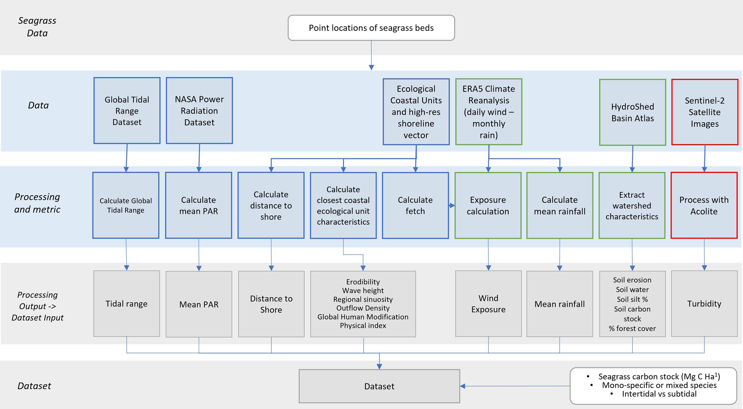
Workflow diagram of spatial data sources used in the final training dataset (input to Figure 2). Datasets and processing flows are coloured as per analysis: green boxes processed in Google Earth Engine, red boxes processed by Plymouth Marine Laboratory hosted MageoHub (MAssive GPU Cluster for EO).
2.2.1 Climatic variables
Climatic variables of rainfall, pressure and air temperature were derived from the ERA5 climate reanalysis monthly dataset (Copernicus Climate Change Service (C3S), 2017) using Google Earth Engine. As this dataset has a resolution of 27.5 km, the pixel value that the seagrass bed is located in was extracted. Monthly averages were extracted for each variable for 10 years between 2010 and 2020. Metrics across the whole period were calculated for the mean and variance in the 10-year dataset as a representation of the climatic environment seagrass beds are located in. The all-sky surface photosynthetically active radiation (PAR) monthly means between the beginning of 2001 and end of 2022 were extracted from the NASA Power Radiation Dataset (The Prediction of Worldwide Energy Resources (POWER) project1) accessed via AWS Open Registry. Monthly means of PAR at a spatial resolution of 1.0° latitude by 1.0° longitude across the whole timeframe were calculated for each seagrass location.
2.2.2 Wave exposure
Wave exposure was calculated as a combination of fetch, wind speed and direction. Firstly, fetch was calculated for each seagrass site along 16 bearing lines based on equal intervals of 22.5 degrees using the R package, Waver2. To represent the intricate shape of the shoreline, a high-resolution global shoreline vector was obtained from Coastal Ecological Units dataset (Sayre et al., 2019) in the ESRI Living Atlas (ESRI Living Atlas of the World, 2021) which was derived from annual composites of 2014 Landsat satellite imagery. Next, wind direction and wind speed (calculated from the 10 m u and v components of wind) were extracted from the ECMWF ERA5 Daily Climate Reanalysis in Google Earth Engine (python API) between 2017 and 2020 (Copernicus Climate Change Service (C3S), 2017). The frequency of wind blowing on each bearing line was calculated with the mean wind velocity.
An index of wave exposure was calculated for each seagrass site using the method by La Peyre et al. (2014), by taking the product of the mean wind speed, frequency of wind direction and fetch along each bearing line to produce a final exposure value for each site:
This analysis was repeated using the upper quartile of wind speeds to calculate an extreme wave exposure index to capture the impact for sites that are disproportionately affected by high wind events. In the final dataset, extreme exposure was removed due to the high correlation between both metrics.
2.2.3 Tidal range
The tidal range in meters was extracted for each seagrass bed from the Global Tidal Range dataset in the ESRI Living Atlas3. This dataset computes tidal ranges using the FES2014 model data obtained from AVISO, a compilation of satellite altimetry data4. A small number of seagrass beds were not covered by the map extent where they were upstream of an estuary in which case the nearest tidal range value was extracted.
2.2.4 Water attenuation, turbidity, suspended particulate matter and chlorophyll parameters
A range of ocean color parameters (Secchi depth, slope of particle backscattering () and diffuse water coefficient (Kd) suspended particulate matter, turbidity, chlorophyll-a) were derived from Sentinel-2 satellite imagery using ACOLITE algorithms. The ACOLITE processor, developed by the Royal Belgian Institute of Natural Sciences, and refined for use with Sentinel 2 imagery (Vanhellemont and Ruddick, 2016) is an image processor that performs atmospheric correction and additionally can process several parameters derived from water reflectances. It employs a dark spectrum fitting atmospheric correction method designed to give improved results in turbid waters. Sentinel-2 tiles required for processing were identified using QGIS by comparing sampling points and the Sentinel-2 granule boundaries. A 20 km buffered box was created around each point to produce extraction areas. Where there was more than one seagrass site per scene, a larger bounding box was drawn around the sites. The identified Sentinel-2 scenes were downloaded from the Google Earth Engine Catalogue from June 2015 to June 2022 (i.e. all datasets up to the point of processing). This included 83 tiles and 86,044 level 1C Sentinel-2 scenes.
Atmospheric correction was undertaken with ACOLITE using default settings. An ACOLITE base configuration file was created and used for each scene with the area modified as needed. Scenes were processed using ACOLITE QAA-pq3aa algorithm (Pitarch and Vanhellemont, 2021) for Secchi depth, Kd and ; using the NeChad et al. (2016) algorithm for suspended particulate matter and turbidity; and chl_oc3 and chl_re_gons algorithms for chlorophyll-a (Gons et al., 2002). Processing was undertaken on MAGEO (Massive GPU cluster for Earth Observation) supercomputer by NERC Earth Observation Data Acquisition and Analysis Service (NEODAAS) resulting in 67,371 scenes.
The median value of a 5x5 pixel area was taken for each seagrass site for each processed variable to reduce noise/smooth values within an area representative of the bed. Values of each variable were averaged by month to create a seasonal profile and reduce the impact of data gaps due to cloudy scenes. For each variable, the annual mean was calculated. Due to the high correlation between these variables, only annual mean turbidity was retained in the final dataset.
2.2.5 Terrestrial soil types and land-use
Using the WWF Hydrosheds Atlas5 (Linke et al., 2019), soil types (% silt, carbon stock, soil water) and land use characteristics (% forest cover, max slope) were extracted from the nearest watershed (level 12) to the seagrass location in Google Earth Engine using the python API (see Table 1 Supplementary material for dataset details). To represent the influence of the terrestrial zone on the seagrass bed, the planar distance from the seagrass bed to shore was calculated in Python using the ECU shoreline dataset as the coastline vector (Sayre et al., 2019).
2.2.6 Ecological coastal units (mean significant wave height, GHM, sinuosity, erodibility, outflow density, climatic zone)
Ecological variables of the nearest shoreline segment to each seagrass bed were extracted from the Ecological Coastal Units (ECU) dataset (Sayre et al., 2022). The ECU dataset was developed by the US Geological Survey (USGS) in partnership with Esri and the Marine Biodiversity Observation Network (MBON). The dataset represents the worlds coastline, segmented into 1 km stretches, of which each is attributed with values from ecological variables including erodibility, mean significant wave height, outflow density, regional sinuosity, global human modification, physical and temperature moisture index. Here global human modification (GHM) is a metric of the relative human influence on a location based derived from 5 anthropogenic stressors: human settlement (population density, built-up areas), agriculture (cropland, livestock), transportation (roads, rail), mining and energy production and electrical infrastructure (power lines, night-time lights) (Sayre et al., 2022).
2.2.7 Coastal typology
Coastal typology from the ‘Worldwide typology of nearshore coastal systems’ (Dürr et al., 2011) was used for an indication of the type of coastal environment each seagrass bed was located in. The seagrass locations were spatially joined, and the ‘nearest’ typology selected: small deltas, tidal systems, lagoons, fjords, large rivers, karstic and arheic coasts.
2.3 Feature selection and pre-processing
A final dataset was created by combing all derived environmental variables with the carbon stock for each seagrass location. To improve the interpretability of the final model, single variables of pairs where the correlation was greater than 0.77 (representing a natural break) were iteratively removed. This included removal of extreme wave exposure, Secchi depth, turbidity and chlorophyll-a. Preference was given to ecologically explanatory variables that support interpretability, without implying causal inference. This step also helped ensure that SHAP analysis could more reliably attribute importance to individual predictors by reducing redundancy among highly collinear variables. The remaining dataset comprised of 21 variables including habitat and species type (mixed or mono-species bed) (see Supplementary Material, Table S1). Categorical variables were encoded with one-hot-encoding, the dataset was randomly split into a train and out-of-sample test set with an 80:20 split. The held-out test set was reserved exclusively for final model evaluation to assess generalization performance on unseen data. Due to the long-tailed distribution, the response variable was log transformed to stabilize the variance.
2.4 Model development
Decision trees and ensemble methods were used to develop a model to predict Corg stocks from environmental predictors (Figure 2). Decision trees and ensemble methods were selected for their ability to handle mixed data types (both numerical and categorical variables), capture non-linear relationships, being robust to outliers, and have been shown to handle small datasets well (Elith et al., 2008). Additionally, for this study ease of interpretation was important for transparency and explainability to end-users to understand which predictors are driving carbon storage (Elith et al., 2008). A range of regression tree methods from the python (v.3.11.7) scikit-learn package (Pedregosa et al., 2011) were tested for their predictive performance from simple decision trees to ensemble and boosted methods and results compared. Models were trained using 3-fold cross validation on the training set (80%) to evaluate performance and to select optimal hyperparameter values using grid search. Hyperparameters are user-defined settings that influence how a model learns, such as those controlling tree structure or sampling strategy. As the models were prone to overfitting, model complexity was constrained during the grid search by tuning hyperparameters such as ‘max_depth’ and ‘min_samples_split’, which control tree structure. Additionally, randomness was introduced within XGBoost using ‘colsample_bytree’ parameter to enhance robustness to noise. Since each algorithm has a distinct set of hyperparameters, it was not possible to define a single unified grid search across all models. However, where hyperparameters were shared across models, such as ‘max_depth’, the same broad search range was applied to ensure consistency in model complexity constraints. The best performing models for each method were re-run within a 3-fold cross validation to extract performance scores (r-squared, root mean squared error) and scored against the out-of-sample test set (20%). This nested validation approach allowed us to tune models while preserving an independent test set for unbiased performance assessment.
Figure 2
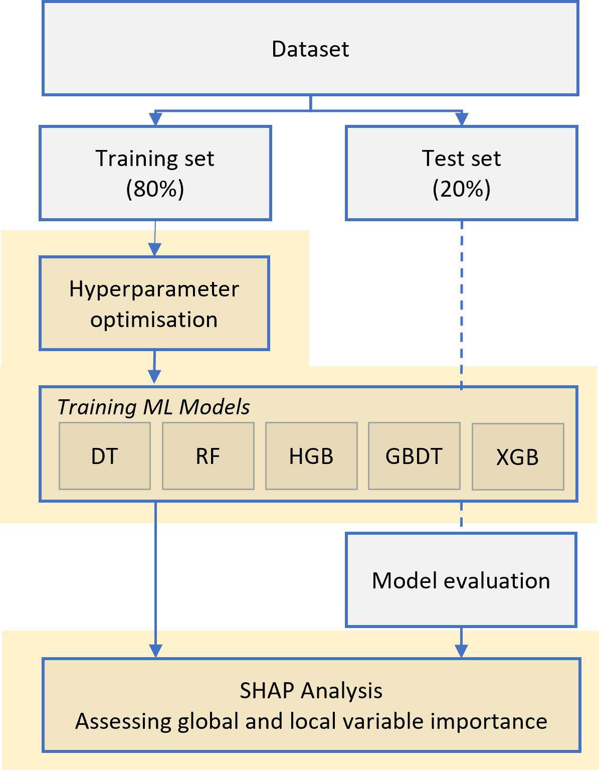
The modelling workflow for predicting carbon stocks in seagrass beds. ML Model abbreviations: DT, Decision Trees; RF, Random Forests; HGB, Hist Gradient Boosting; GBDT, Gradient boosting Decision Trees; XGB, XGBoost.
2.5 Explanatory analysis
SHAP analysis (Shapely Additive exPlanations) was used to interpret the model and infer insights about the significance of features to the model’s output (Lundberg et al., 2017). As ensemble methods (such as XGBoost and Random Forest) combine the results of many individual learners it is not possible to visualize how the algorithm is generating the result. Explainable ML aims to explain how such models make predictions which gives insight into what features are driving predictions. SHAP uses Shapley values (Shapley, 1953), a method derived from cooperative game theory, to explain the output of any ML model by attributing a ‘players’ contribution to the game (Lundberg et al., 2017). SHAP values are therefore measures of the contribution that each feature has on the outcome of the model.
SHAP analysis was undertaken within a cross-validation scheme by computing representative SHAP values for the test sets. This method produces more robust understanding of the average behavior of the model’s interpretability in comparison to single repeats that can produce unstable results. Reported SHAP values are therefore the average impact on the model output across 10 runs.
3 Results
3.1 The dataset
The collated dataset of Z. marina Corg stocks comprised of 176 sites from datasets published between 2016 and 2023 (available at https://doi.org/10.5281/zenodo.15864691). Sites cover 18 eco-regions across the temperate realms of Z. marina extent: the Temperate Northern Pacific and Temperate Northern Atlantic (Figure 3). There was not an even distribution of sites sampled across the known extent for Z. marina. Samples are skewed towards the northern European seas (n=93) and cold temperate northeast Pacific (n=56) with lower representation in Mediterranean, Lusitanian, Black Sea and Northwest Pacific eco-regions (χ² = 344.98, p< 0.001). Sites from the North Sea alone make up over 30% of the total dataset. Additionally, the distribution of intertidal and subtidal samples was examined across both ecoregions and biogeographic provinces. Chi-square tests of independence revealed significant associations between habitat type and both ecoregion (χ² = 64.85, p< 0.001) and province (χ² = 52.45, p< 0.001). These results indicate that intertidal samples were not evenly distributed across geographical areas, with certain regions and provinces being disproportionately represented.
Figure 3
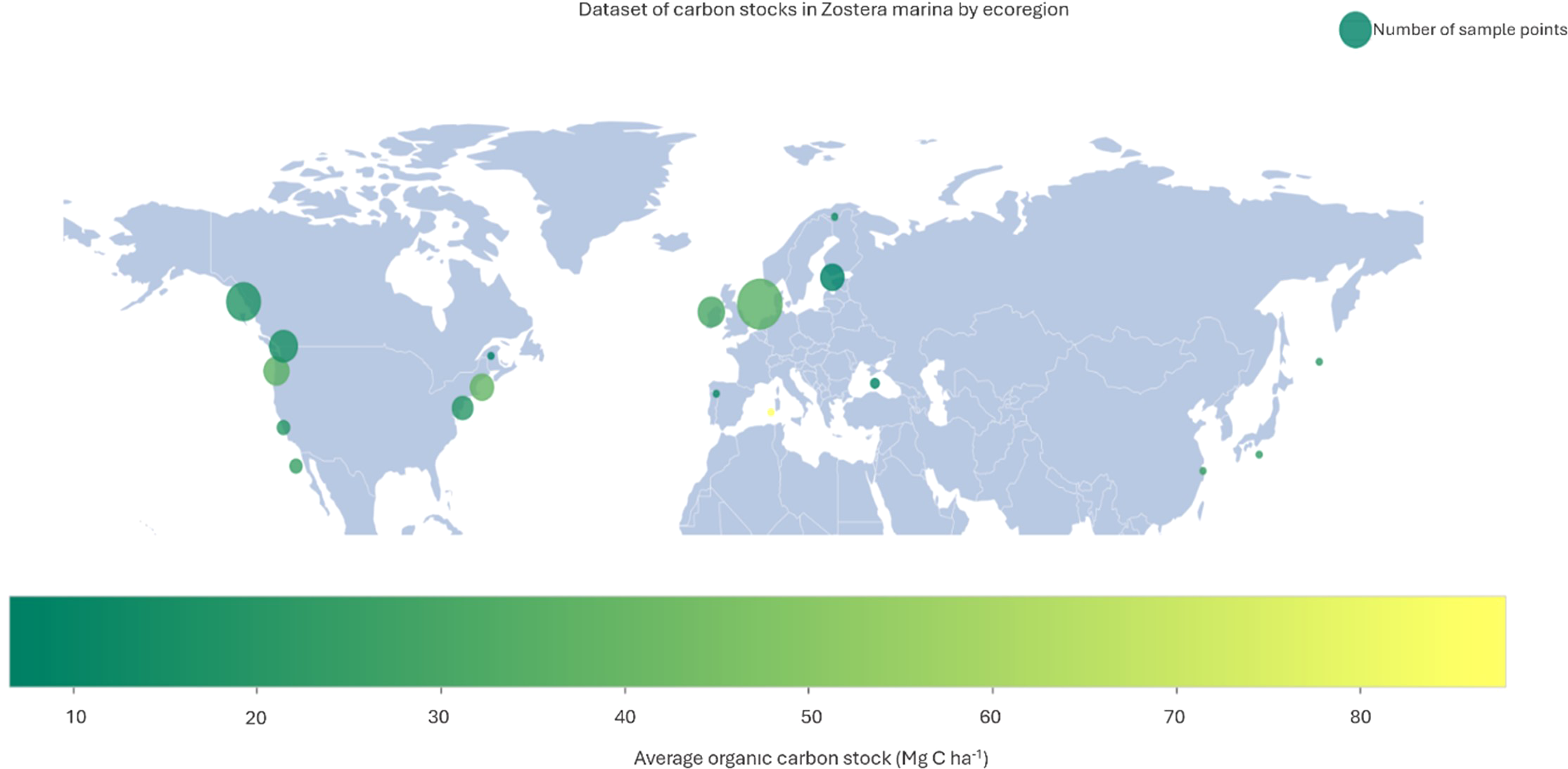
Map of the distribution of Z. marina sample sites showing the number of sites per Ecoregion coloured by mean carbon stock (Mg C ha-1) to 25 cm depth. (Yellow = higher carbon, green = lower carbon). The size of the marker represents the number of sample points within each Ecoregion.
Total mean carbon stock across all regions in the top 25 cm of sediment was 23.85 Mg C ha1. However, the variability in carbon storage size was substantial between sites ranging from 3.18 Mg C ha1 to 105.77 Mg C ha1. The mean carbon stock in subtidal beds (n = 119) was marginally higher at 24.1 Mg C ha-1 compared to 23.3 Mg C ha-1 for intertidal beds (n = 57), though this difference was not statistically significant (p = 0.8273). In contrast, carbon stocks differed significantly across ecoregions (p< 0.001), indicating that biogeographical context, and therefore environmental conditions, play an important role in carbon storage potential (Figure 4). The warmer eco-regions (Warm Temperate northeast Pacific and Warm Temperate Northwest Pacific) had higher average carbon stocks than the cooler seas when aggregated by Province. However, differences across provinces were not statistically significant (p = 0.2720) (Supplementary Material Figure S2 for Ecoregion). Additionally, all regions exhibit large within-group variations in carbon stocks consistent with previous studies (Prentice et al., 2020; Röhr et al., 2016, 2018).
Figure 4
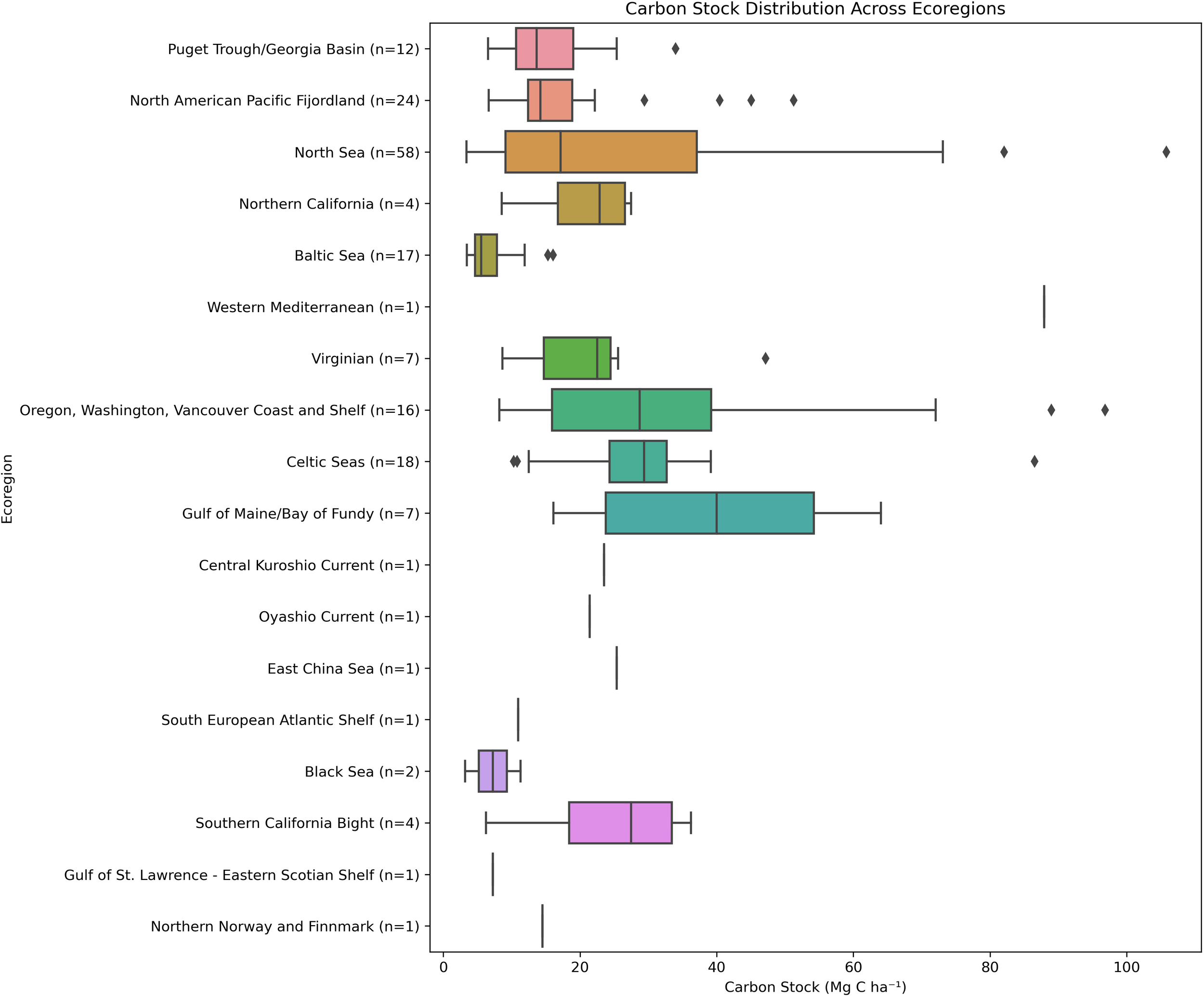
Distribution of Z. marina organic carbon stocks (Mg C ha-1) in the top 25cm of the sediment by Ecoregion. The number of seagrass locations in each ecoregion are shown in brackets. The boxplots show the three quartile values of the distribution, and the “whiskers” extend to points that are within 1.5 interquartile range of the lower and upper quartile. Observations falling outside of this range are displayed independently. Differences in carbon stock across ecoregions were statistically significant (Kruskal-Wallis p-value< 0.001).
After the removal of highly correlating variables, the highest correlating pairs in the final dataset were soil carbon stock and mean rain (+0.76), soil water and mean PAR (-0.70) and human modification and soil carbon stock (-0.63) (Figure 5). The dataset was split 80% for the train set and 20% as an out-of-sample test dataset resulting in a dataset size of 140 and 36 samples respectively. The response variable train dataset ranged from 3.18 Mg C ha1 to 105.77 Mg C ha1 with a mean of 18.12 Mg C ha1. The test dataset was within the ranges of the train dataset ranging from 3.39 Mg C ha1 to 86.50 Mg C ha1 and a mean of 15.43 Mg C ha1 (see Supplementary Material Figure S3).
Figure 5
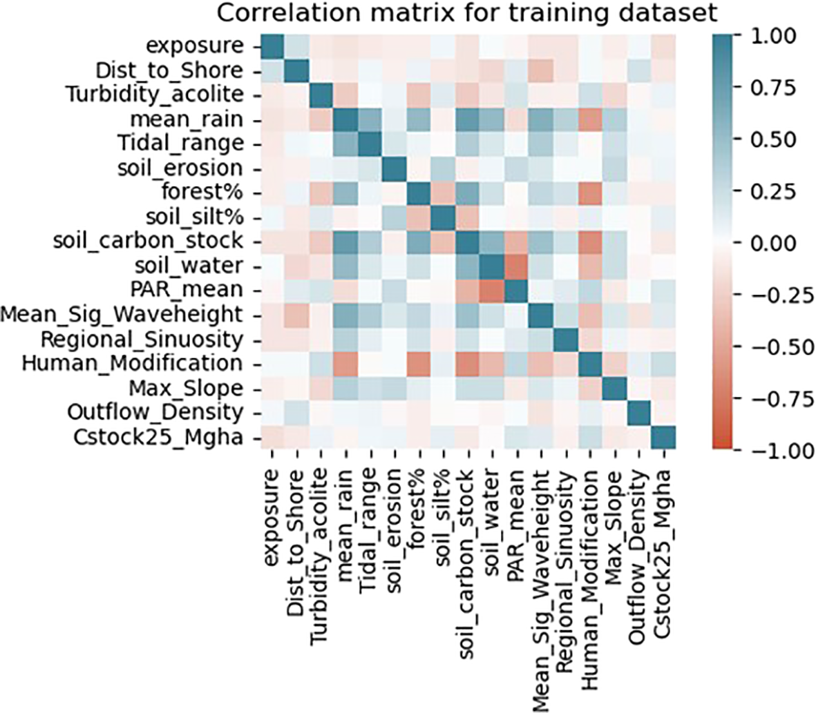
Correlation matrix of final continuous numerical variables in the train dataset. Darker colors are indicative of higher correlation with blue showing positive correlation and red negative correlation. Note that categorical variables are not included.
3.2 Model evaluation
The optimized ML models were evaluated against the test dataset using performance metrics, specifically the coefficient of determination (r2) and root mean square error (RMSE) (Figure 6 and Supplementary Material, Table S2). The evaluation revealed a significant disparity in performance between the simplest decision trees and the more complex gradient boosted regression trees. The simple decision trees (‘decision trees’) performed sub-optimally with overly simplistic trees resulting in average r2 validation scores close to zero. Conversely the validation and test scores indicated that the best performing models were Random Forests, Gradient Boosting and XGBoost. These models have very similar scores (r2 0.36, 0.35, 0.37 on the test set respectively) but XGBoost and Gradient Boosting have marginally improved fit at the outer ranges of the response variable (Supplementary Material, Table S2).
Figure 6
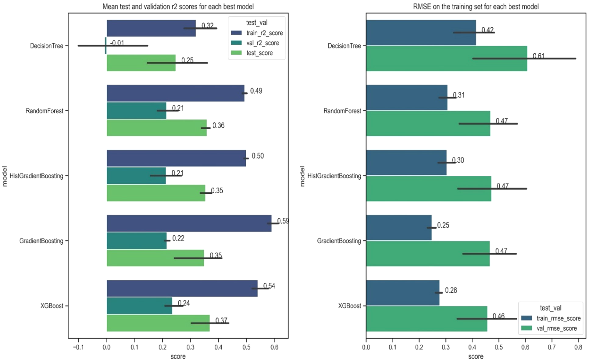
Model evaluation plots showing for each model (left) the r-squared for the train, validation and test sets respectively; and (right) the logged RMSE scores for the train and validation sets respectively. The error bars show the uppermost and lowest values of the scores produced during cross-validation.
Based on overall performance, XGBoost was selected as the preferred model providing a marginal improvement in performance and good balance between bias and variance. Consequently, we report that the final combination of 21 variables can predict 54% of the variability in Corg stocks in Z. marina beds in the train dataset, and 37% of the variability in the test set. The model, however, does underpredict in the upper 5% of sites and has an average residual (actual – predicted) on the whole dataset of 12 Mg C ha-1 (Supplementary Material, Figure S4). Moran’s I for model residuals was –0.006 (p = 0.314), indicating no significant spatial autocorrelation (Supplementary Material Figure S5).
3.3 Model explanation
3.3.1 Feature importance
SHAP plots (Figures 7, 8) provide insights into the importance of features and their impact on the final model prediction. The top six features driving predictions are human modification, exposure, tidal range, mean significant wave height, mean rainfall and turbidity. Seven variables account for over half (52%) of the SHAP forcing. Least predictive variables are marine physical environment categories (i.e. an integrated measure of sea surface temperature, oxygen and salinity), intertidal or subtidal beds, erodibility, typology and mixed or monospecific beds. Human modification is the most predictive feature with higher modification indicative of higher carbon stocks. Higher exposure has a negative correlation, with higher exposure predicting lower carbon stocks. Lower tidal range correlates with lower carbon stocks and higher values of mean significant wave height, rainfall and turbidity are also associated with lower carbon stocks. Whether a bed was intertidal or subtidal was not a predictive feature of a beds carbon stock. However, to identify differences in how features drive predictions between bed types, SHAP values were split by the two groups (Figure 9). Hydrodynamic features exhibited slight variations, with exposure and tidal range being more significant in the subtidal beds than intertidal beds. Conversely human modification at the coast was marginally more predictive for intertidal beds. The climatic features of mean rainfall were also slightly more predictive for subtidal beds whilst PAR had a greater impact on intertidal beds.
Figure 7
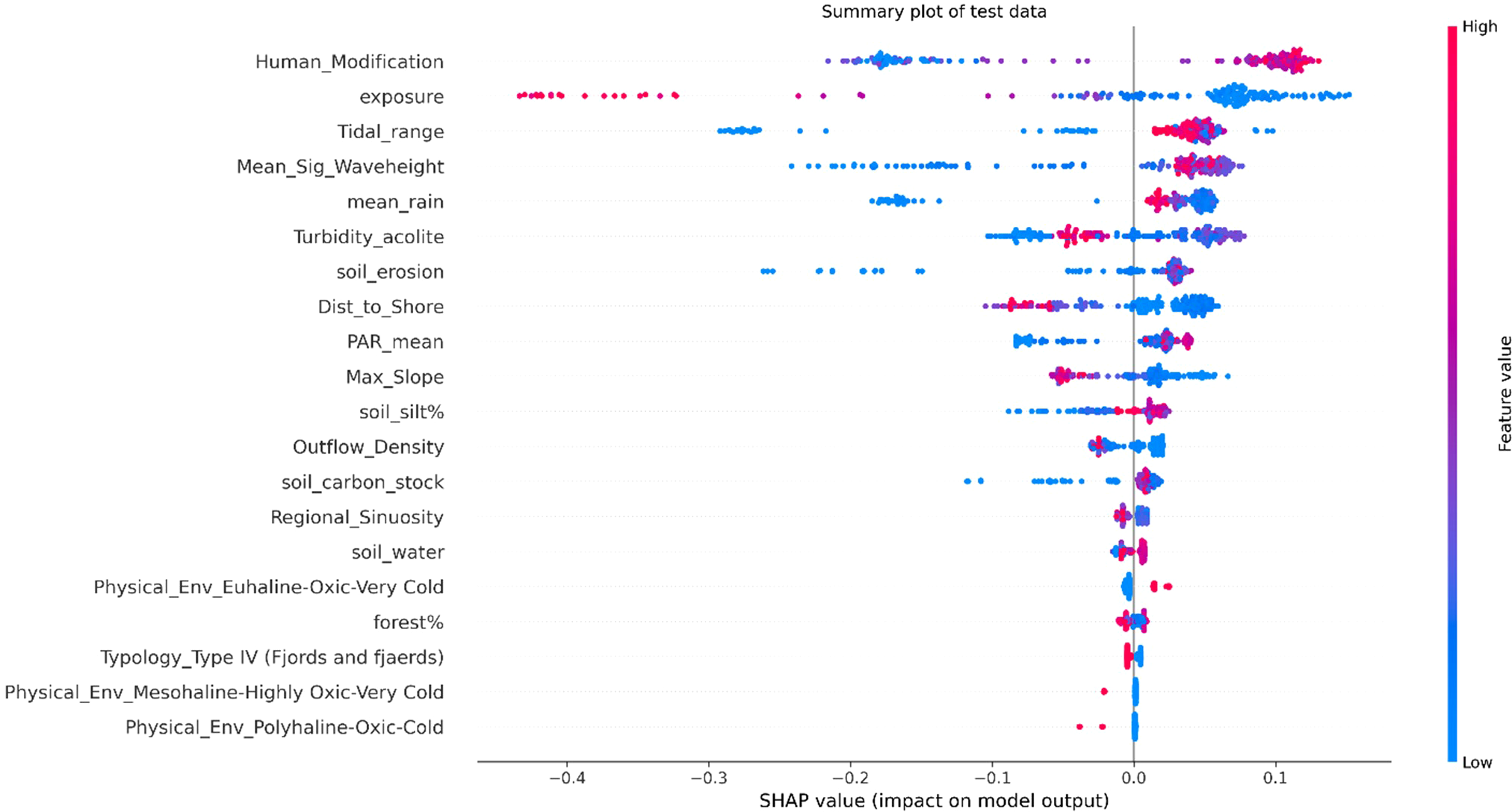
SHAP summary plot for test data showing feature importances of top 20 features (from top to bottom). The plot illustrates the magnitude and direction of each features impact on the model predictions (from left to right). Red dots indicate high feature values, while blue dots indicate low feature values. The position of each dot along the x-axis represents the SHAP value, indicating the strength and direction of the features impact. Note the encoding of categorical variables.
Figure 8
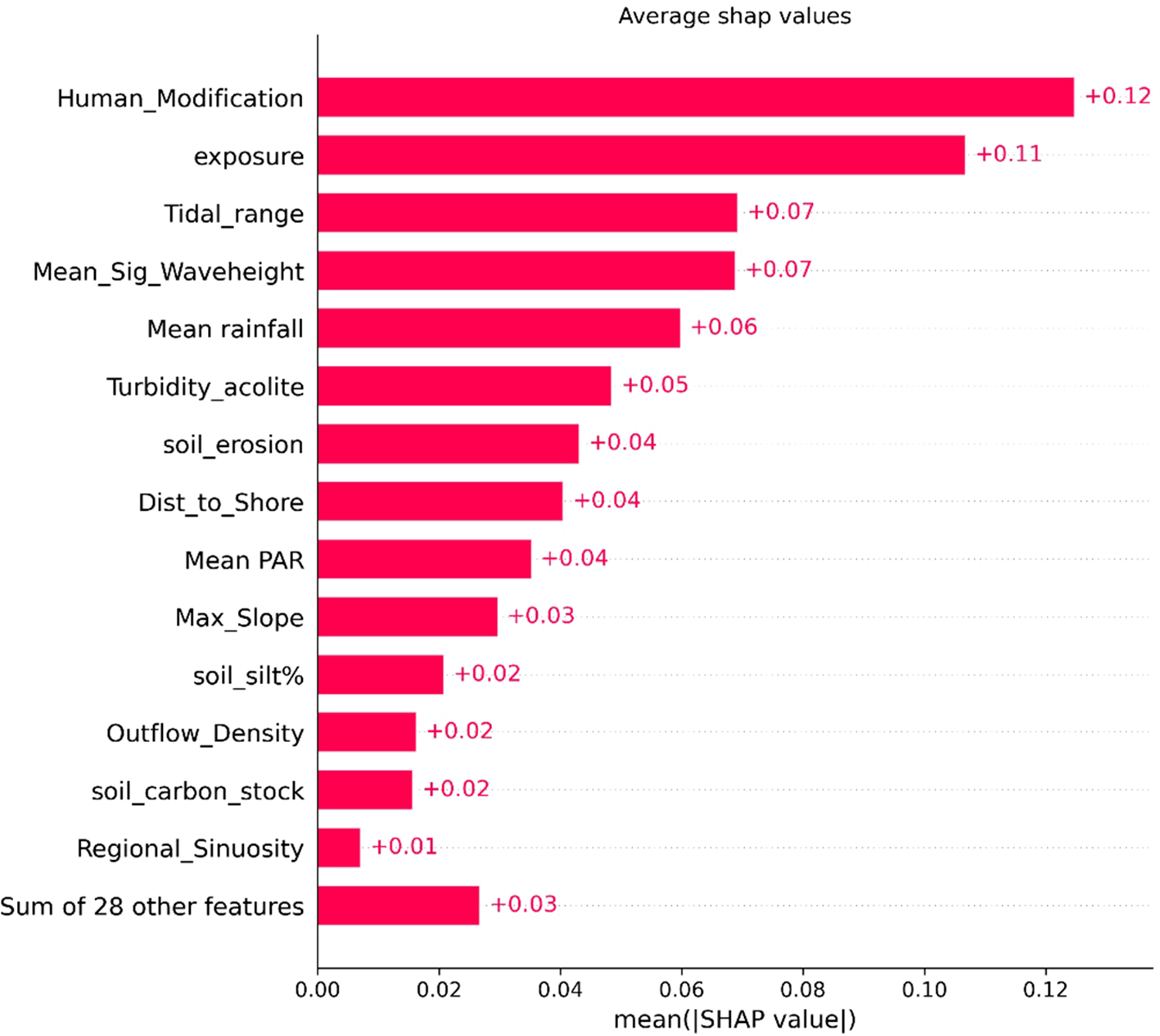
SHAP bar plot showing global feature importance for the test set, with each bar representing a feature’s mean absolute SHAP value. Features are ordered by their impact on the model’s predictions, with the most influential at the top. Here, the dataset corresponds to 42 features due to the encoding of categorical variables.
Figure 9
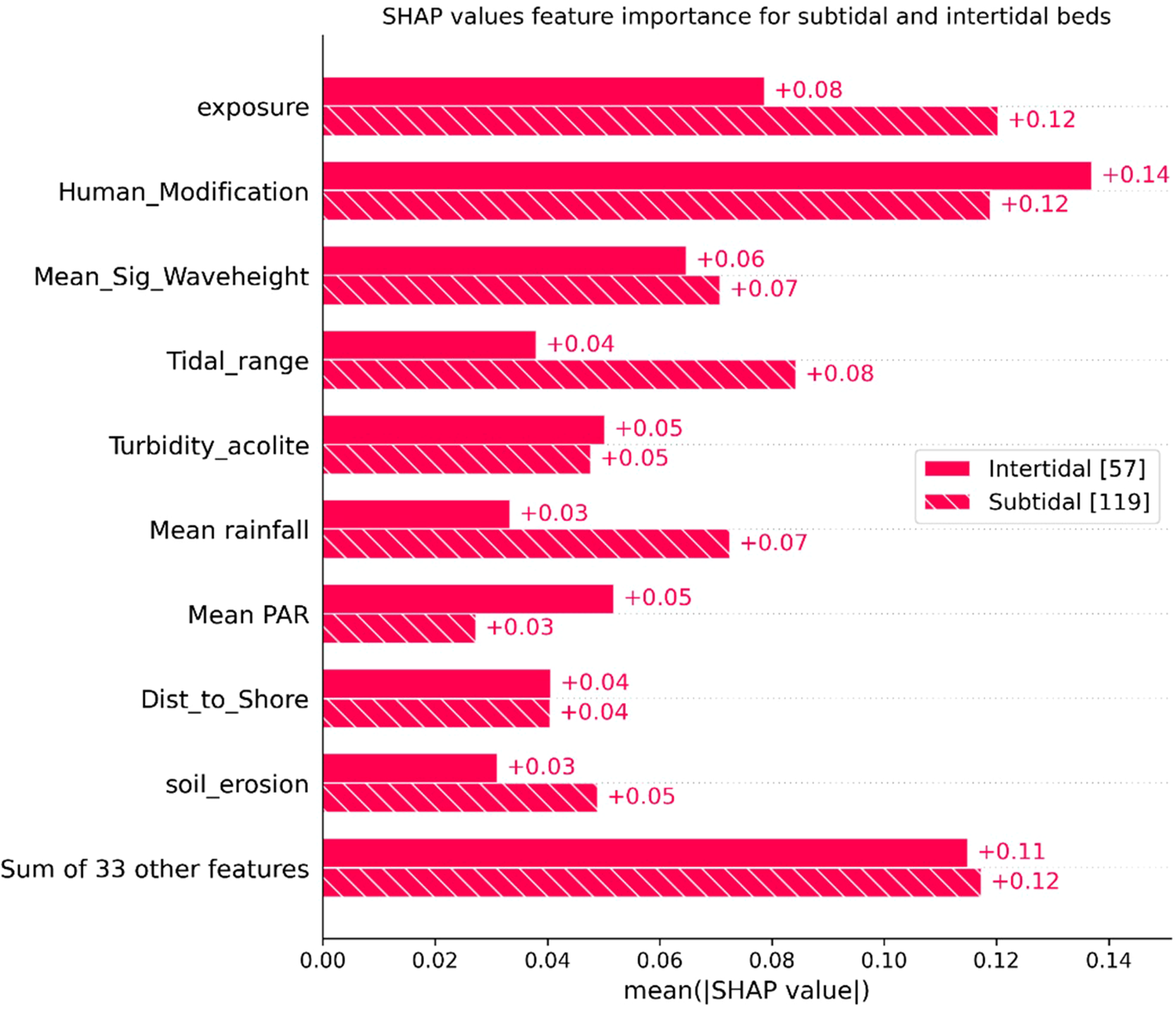
Bar plot illustrating the mean SHAP values for each feature, highlighting their importance across subtidal and intertidal beds. Here, the dataset corresponds to 42 features due to the encoding of categorical variables.
3.3.2 Variable dependence
Dependence plots represent a variables SHAP value for a given seagrass bed showing the effect a single feature has on the model predictions (Figure 10) (Lundberg et al., 2017). Human modification at the nearest coast creates a threshold effect with low carbon stocks at low human modification values but shifting into higher carbon values when passing a threshold of around a 0.3 in the human modification index. Exposure suggests a more linear relationship with increasing exposure resulting in lower carbon stocks, except for the lowest exposure levels which has an initial dip.
Figure 10
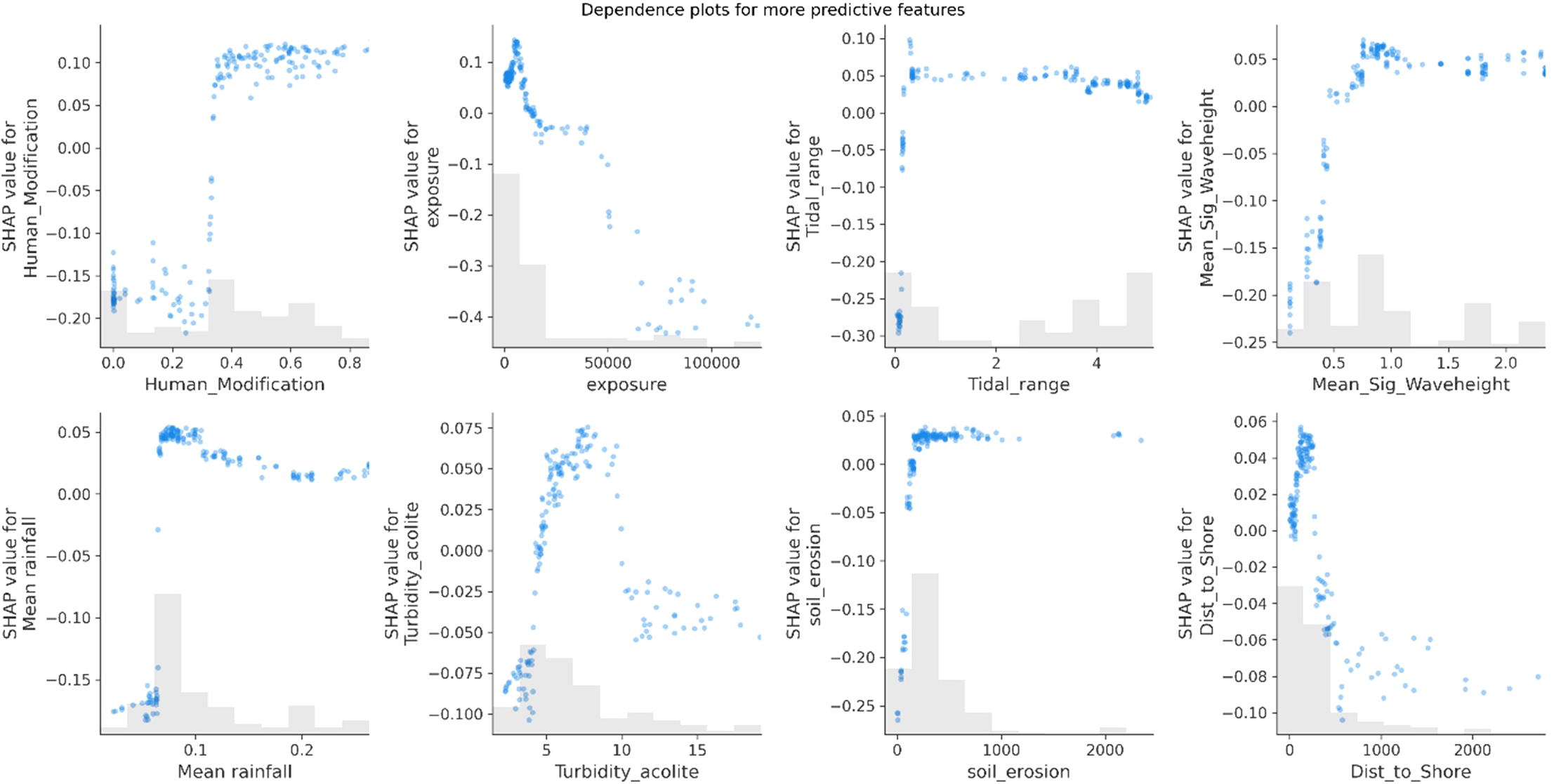
SHAP dependence plots for the 8 most predictive features, illustrating the relationship between the value of a specific feature and its corresponding SHAP value. The x-axis represents the feature values, while the y-axis shows the SHAP values. Each blue dot represents an individual data point, highlighting how the feature value affects the prediction for that instance. The grey bars at the bottom of the plot represent the distribution of the feature values, providing a histogram that shows how frequently each value occurs in the dataset.
Tidal range, mean significant wave height, mean rainfall and soil erosion all exhibit a similar pattern with carbon stocks whereby at the low ends there are low carbon stocks but go through a rapid step change at a threshold point to correlate with higher carbon stocks. Distance to shore shows a general negative correlation with carbon stocks and turbidity shows a positive correlation with increasing carbon stocks up to a level of approximately 8 FTU after which carbon stocks decline. It should be noted that this dataset is based on a range of environmental conditions within which seagrass beds are considered healthy and productive and does not include those which are being negatively affected by stressors and threats. Therefore, it may be expected to see declining carbon stocks as turbidity and human modification levels increase further, as a result of inhospitable environmental conditions and degrading habitats.
4 Discussion
4.1 Key findings
As far as it is known, this study has collated the most comprehensive dataset of Z. marina carbon stocks and associated environmental conditions available. Furthermore, it is believed this is the first attempt to predict carbon stocks in Z. marina seagrass beds at scale from EO-derived and other globally available datasets with ML methods. Similar research in other species includes: boosted regression trees to predict carbon stocks for mangroves and seagrass beds in Queensland, Australia using regional datasets (Duarte de Paula Costa et al., 2021, 2023), linear mixed effects models to predict carbon stock from in-situ sampled species-specific traits (Kennedy et al., 2022), and generalized additive models (GAM) using the BioOracle dataset in Florida Gulf Coast (McHenry et al., 2023a). The strength of the approach demonstrated here lies in the ability to easily scale up spatially and across species. In comparison to the reliance on in-situ measured carbon stocks or regionally specific datasets, the approach presented here makes use of readily and globally available data to explore the potential to develop a globally applicable model for multiple seagrass species.
Based on the out-of-sample test set, the best model, XGBoost, predicts 37% of the variance in carbon stock. Simple decision trees significantly underperform and do not generalize well as seen from the poor validation scores. This underperformance can be attributed to their limited ability to capture complex patterns and interactions within the data. The ensemble methods performed similarly to each other, outperforming simple decision trees. The superior performance of these models can be attributed to their ensemble techniques which produce improved predictive accuracy by combining multiple weak learners to form a more robust predictive model and avoid overfitting. Whilst all models underperform at the upper and lower ends of the distribution, combining results from multiple trees goes some way to mitigating errors and biases associated with fewer samples at the outer edges of the dataset thereby improving the overall prediction performance (Chen et al., 2024). The gradient boosting methods are a competitive alternative to random forests as they build shallow trees that underfit individually in comparison to deep trees that overfit individually. In contrast to random forests that train decision trees independently and majority voting on the output, XGBoost trains many decision trees sequentially adjusting with the error from the previous tree. XGBoost has the benefit of many hyperparameters available for optimization, including regularization hyperparameters to reduce overfitting. In combination XGBoost is therefore a high performing model which is more robust to imbalanced or noisy data. Overfitting in XGBoost was controlled by constraining the model complexity (e.g. max depth), adding randomness (e.g. subsampling columns per tree) and regularization (e.g. alpha) to make the training robust to noise. The need to control for overfitting in this way suggests there is a high level of noise within the dataset indicative of the complex natural system that is not easily explained by a few features (Lucas, 2020).
The model here does not perform as well as the boosted regression trees model of (Duarte de Paula Costa et al., 2023) who found 9 environmental variables predicting 65% of the variability in Corg stocks in seagrass meadows (mean squared error = 16.94 and correlation = 0.76 between predictive values and the independent dataset, dataset size n= 268). Solar radiation, distance to the closest estuary and water depth accounted for most of the variability in their Australian seagrass meadows (Duarte de Paula Costa et al., 2023). The difference in predictive performance could be due to the different drivers occurring in tropical and temperate systems and the seasonal variability in temperate meadows (Dahl et al., 2020b; Davies et al., 2024). Additionally, modelling a larger geographical distribution is inherently more challenging. It will naturally encompass larger variance and noise in the input data which can increase the risk of overfitting particularly when working with relatively small datasets. This may require the inclusion of additional predictor variables to better account for biogeographical variation.
Predictor variables of bed shear stress, water current speed and water depth (Duarte de Paula Costa et al., 2023) were absent from our model due to the unavailability of global datasets with an appropriate resolution for the coastal regions studied. The effect of depth on carbon is unclear in the literature being reported as having no significant effect on carbon storage (Mazarrasa et al., 2018) or decreasing carbon storage potential with greater depths (Serrano et al., 2014). Other variables could also be important that are not accounted for in the model. pH has been identified as a driver of carbon storage potential with carbon content decreasing in high pCO2 and low pH conditions (Vizzini et al., 2019) as well as the interaction between other habitats (e.g. oyster reefs) likely due to the source of allochthonous carbon and reduced wave attenuation effects (McHenry et al., 2023a).
Most of the predictor variables within the model are at the regional or local scale. Meadow-scale interactions have also been shown to have some influence on carbon stocks. Seagrass bed characteristics influence the hydrodynamic forces affecting the bed by reducing water velocity across the bed (Fonseca and Cahalan, 1992), seagrass cover (McHenry et al., 2023a), seagrass species traits (Kennedy et al., 2022) and the seagrass size itself has been shown to have a positive effect on carbon stocks (Gullström et al., 2018). However, bed characteristics were not included in the model here as they are often not consistently measured or reported alongside carbon datasets. Furthermore, the aim of this study is to explore alternative approaches to enable wider quantification of carbon stocks to be made, reducing reliance on extensive field measurements and support application to future restored beds with unknown bed characteristics.
4.2 Factors driving carbon stock
In addition to making predictions on the carbon stock of seagrass beds, understanding which environmental factors drive carbon storage is of considerable importance and relevance to policy and management. The use of explainable ML for ecological studies is important to facilitate discussion and bridge the gap between data scientists and ecologists (Cha et al., 2021) providing insights into how algorithms function. It is well recognized that more transparent, interpretable or explainable algorithms are more likely to be trusted and therefore used by end-users (Ashoori and Weisz, 2019; Brundage et al., 2020; Thiebes et al., 2021).
It should be noted that the purpose of the models trained here are for solving prediction problems and are not inherently causal models (SHAP, 2024). Therefore, SHAP provides a tool to understand how variables are used to make predictions but do not accurately answer causal questions making it inappropriate to measure causal impacts for management decisions or predict changes in the future. The discussion presented here provides a ‘sense check’ and transparency of how the model is making predictions compared to other empirical and modelled studies investigating factors driving carbon stock.
Results show that the most important features predicting carbon stock were variables related to the hydrodynamic environment (exposure, tidal range, mean significant wave height and turbidity), climate (rainfall) and the influence of land-use (human modification, distance to shore). In contrast to Duarte de Paula Costa et al. (2021), who found soil type of the nearest land point accounted for most of the variability (47.5%) in Corg stocks, in the model here soil type of the nearest watershed was not very predictive. The predictive variables of human modification, turbidity, soil erosion and distance to shore, all suggest that the availability of sediment is more predictive than the soil type. Coupled with the hydrodynamic environment of exposure, tidal range and mean significant wave height which affect the conditions for decomposition. Climatic variables were less important except for rainfall, which additionally can be explained as a factor enhancing terrestrial sediment availability from run-off. This is in contrast to Duarte de Paula Costa et al. (2021), who identified solar radiation (14.8%), temperature (7.8%) and rainfall (3.6%) contributed to the variability suggesting the climatic impacts may be more important in the more productive tropical systems compared to temperate systems (Carruthers et al., 2002). McHenry et al. (2023a) found that just three features explained most of the variation in carbon stocks in the Florida Gulf Coast: total cover of seagrasses, distance from river outlet and proximity to oyster reefs. These likely explain the availability of Corg and estuarine influence on deposition of allochthonous carbon, which seems to be especially relevant for Z. marina meadow carbon accumulation.
Human modification was the most predictive variable showing a positive correlation of higher human modification with higher carbon stocks. Here, human modification is estimated as a proportion of a given location (a pixel) that is modified based on 5 stressors: human settlement (population density, built-up areas), agriculture (cropland, livestock), transportation (roads, rail), mining and energy production and electrical infrastructure (power lines, nighttime lights) (Sayre et al, 2021). Human impact has been identified as a key factor influencing carbon stocks. Eutrophication caused by nutrient inputs from human activity contributes as a source of allochthonous carbon such as phytoplankton and organic detritus (Duarte, 1995) particularly in sheltered meadows (Mazarrasa et al., 2018). Allochthonous carbon is considered to contribute up to 50% of the total carbon buried in temperate seagrass sediments (Kennedy et al., 2010) and moderate nutrient inputs may benefit seagrass productivity (Powell et al., 1989). It should be noted that whilst anthropogenic activity can be a major stressor driving seagrass declines, all the seagrass beds included within this study here are considered healthy beds and so the relationships here are indicative of seagrass meadows within a healthy range of environmental conditions. This feature is therefore likely predictive due to its effect on the delivery of allochthonous carbon from human activity, agriculture and runoff within healthy limits.
The second most predictive feature, exposure, has been identified in many studies as an important determinant of carbon stocks although with conflicting results. Exposure affects the pattern of sedimentation, sediment resuspension, levels of erosion and bed dynamics (Bradley and Houser, 2009; Hansen and Reidenbach, 2012; Van Keulen and Borowitzka, 2003). Exposure is also closely correlated with sediment properties; mean grain size has been shown to increase with fetch (Mazarrasa et al., 2018), mud content and degree of sorting decrease with wave exposure (Dahl et al., 2020a) and smaller grain sizes coincide with more sheltered environments (Fonseca and Bell, 1998; Murphey and Fonseca, 1995). It was found that the most sheltered sites were correlated with the highest carbon. Sediment grain size and carbon content is widely considered to be a determinant of carbon stocks with finer, siltier sediments increasing anoxic conditions and controlling the level of microbial activity degrading organic matter (Dahl et al., 2016; Lima et al., 2019; Miyajima et al., 2017; Novak et al., 2020; Prentice et al., 2020; Röhr et al., 2016). Conversely, mean significant wave height had an inverse relationship to exposure. Higher carbon stocks have been related to more sheltered areas with lower wave height and high sediment availability (de los Santos et al., 2019; Prentice et al., 2020; Samper-Villarreal et al., 2016). In contrast, Dahl et al. (2020a) found the opposite effect with high hydrodynamic exposure related to higher carbon storage, although these were sites mainly classified as extremely sheltered, a pattern that is seen in the most sheltered sites.
Moderate levels of turbidity were found to be correlated with the highest carbon stocks with lowest carbon stocks being in areas with very low turbidity. However, beyond a threshold level of approximately 8 FTU, higher turbidity resulted in decreasing carbon stocks (Halim et al., 2020) suggesting some suspended sediment is important as a source of organic material for seagrass beds, but too much may be detrimental. Higher turbidity may have negative effects on plant productivity and meadow density due to lower irradiance (Serrano et al., 2014) however, increased seagrass stocks have been attributed to increases in sediment accumulation as a result of land erosion and changes in sea level (Cuellar-Martinez et al., 2020). Surprisingly, several factors commonly reported to influence carbon stocks were not predictive features within the model. Intertidal vs subtidal bed was not a significant predictor for carbon stock. However, exposure and tidal range was more predictive in subtidal than intertidal beds likely suggesting hydrodynamic effects are more predictive for subtidal bed carbon storage. However, the dataset was not balanced between the two bed types with considerably more subtidal samples than intertidal, and intertidal samples were unevenly distributed across regions affecting the model’s ability to predict habitat-related effects.
The marine physical environment, an integrated measure of sea surface temperature, oxygen and salinity, was also one of the least predictive variables. These variables are often associated with variations in primary productivity, which suggests that primary productivity of Z. marina beds is not a significant driver of carbon storage, similarly found by Röhr et al. (2018) who showed that less than 50% of the sediment carbon in Z. marina beds is derived from the seagrass itself.
The variability in regional carbon stocks is large and therefore regional averages are unreliable indicators of potential carbon stocks. Features driving the hydrodynamic and decompositional environment are more indicative of carbon stock than climatic variables. Therefore, extrapolating carbon stock data across regions is unreliable (Röhr et al., 2018; Stevenson et al., 2023). The methods presented here are an improvement on existing approaches and give site-specific estimates based on the unique combination of environmental conditions. It is proposed that this method can therefore be used to derive insights into the spatial variability of carbon stocks to inform carbon accounting and support conservation and restoration decision-making.
4.3 Limitations and future directions
This first attempt to model carbon stocks in Z. marina highlights the inherent complexity of modelling highly variable, global environmental systems. There is a need to balance model complexity with accurate representation of ecological processes. The lack of suitable datasets, both in quality and quantity, limits the wider application of ML methods in ecology (Liu et al., 2018). Here, the train dataset size likely restricts the ability of the model to accurately capture variability. ML models generally perform poorly with extreme values (Lucas, 2020) extrapolating poorly at the edges of response and predictor variables (Elith et al., 2008). As sites with carbon stocks at the extremes are predicted poorly due to the long-tailed distribution of the response variable, improvements could be gained with a larger representation of samples at the upper end of the distribution (Rubbens et al., 2023). Additionally, the spatial distribution of the data was limited by sampling effort per country affecting the generalizability of the model outside these environmental limits. Ongoing sampling of Z. marina beds aims to build a comprehensive evidence base (Graversen et al., 2024), providing additional training data for future modelling efforts and potential to include additional species.
Uncertainty from the heterogenous nature of ecological systems is a pervasive problem (Regan et al., 2002). In this study, uncertainty and variability exists in both the response and predictor variables. The predictor variables are reduced to a single averaged metric that may fail to capture the variability in conditions at and between Z. marina sites. These metrics are also representing present-day conditions which may not be true of the historic conditions that influenced the decomposition of carbon over time or how it may change into the future. Additionally, within the response variable uncertainty arises from averaging carbon stock values from multiple cores across the seagrass bed, losing the meadow spatial variability which is known to vary with distance from the bed edge (Ricart et al., 2017). While efforts were made to include only studies that followed standardized protocols (see section 3.1), some variability in sampling or analytical methods may still contribute to the observed differences in carbon stock values. Probabilistic approaches may therefore be suitable here for future iterations by treating features as variables with distributions rather than fixed values to incorporate uncertainty and variability into the model with potentially more reliable predictions (Reimer et al., 2022).
A broad range of environmental variables were used within the model to capture the variability across the physical, climatic, terrestrial and anthropogenic conditions. Improvements could be gained by including new features of certain predictor variables although these are expected to be marginal. Some datasets are available only at a coarse resolution, are modelled, or have been down-sampled. This loss of detail removes the fine spatial information necessary to accurately represent complex coastal environments, leading to oversimplification and reduced accuracy. As a result, these datasets may not effectively capture local-scale ecological processes, such as within-meadow variability, and aggregation effects can obscure important spatial heterogeneity within coarse grid cells. Due to the intricate nature of coastal systems, high-resolution datasets are essential to accurately capture localized effects that influence seagrass dynamics. Specifically, here the terrestrial soil type variables are currently at a very coarse scale derived from the nearest level 12 HydroBasin watersheds which is not always representative of the feeder watershed to the seagrass bed. These inputs could be improved with aggregated stream flow inputs and smaller watershed delineations. New EO derived datasets are continuing to become available with higher resolution and accuracy offering opportunities to incorporate for improvements in future iterations (e.g. Hydrosheds v2.06, Seabed20307).
5 Conclusion
This study presents an exploratory approach to modelling seagrass carbon stocks at a multi-regional scale using machine learning. The model was able to predict nearly 40% of the carbon variability within a Z. marina seagrass bed from global datasets, with the performance reflecting the challenges of modelling complex ecological systems. Alongside this, a comprehensive dataset of Z. marina carbon stocks with 21 associated environmental variables is presented and made available to the scientific community. Human modification, exposure and tidal range are found to be the most predictive variables of carbon stocks in Z. marina. Features driving the hydrodynamic and depositional environment were more important than climatic variables highlighting the importance of improved methods that consider the unique environmental conditions affecting a given seagrass meadow.
The approach here highlights the challenges of modelling coastal ecological systems which are inherently complex and contain multiple sources of uncertainty. Whilst there are opportunities to improve the predictive performance of the current model through larger and higher accuracy datasets which will become available with time, probabilistic ML methods that can model intrinsic uncertainty may be more suitable for future iterations. Additionally, this study reinforces the need for consistent, standardized carbon stock datasets as training data for the wider application of ML methods in coastal habitat studies with a need to focus future efforts in regions that are least represented in sampling programs. The continual development of high-resolution EO derived datasets in the coastal realm offers additional opportunities for improvements in this area.
The model presented here offers a preliminary method for generating spatially explicit, site-level carbon estimates. Whilst it should not be viewed as a replacement for field-based measurements, it highlights the potential of ML to support carbon accounting efforts, particularly in data-poor regions, and to inform future conservation and restoration planning. Improving model performance will require larger, more representative datasets and the integration of higher-resolution environmental predictors. As data availability and modelling techniques continue to advance, this approach could form the basis for more robust, scalable tools to support blue carbon assessments and guide decision-making in coastal ecosystem management.
Statements
Data availability statement
The original contributions presented in the study are included in the zenodo.org/records/15864691. Further inquiries can be directed to the corresponding author.
Author contributions
NW: Methodology, Visualization, Validation, Conceptualization, Data curation, Writing – original draft, Formal analysis. RA: Supervision, Writing – review & editing. ES: Writing – review & editing, Data curation. RB: Conceptualization, Writing – review & editing, Supervision. RE: Writing – review & editing. CL: Writing – review & editing, Supervision, Conceptualization.
Funding
The author(s) declared that financial support was received for this work and/or its publication. This research was undertaken as part of an EPSRC funded PhD in the UKRI Centre for Doctoral Training (CDT) in Environmental Intelligence: Data Science and AI for Sustainable Futures (grant number: EP/S022074/1). RB is supported by a UKRI FLF (MR/V022792/1).
Acknowledgments
We wish to thank the NERC Earth Observation Analysis and Artificial Intelligence service (NEODAAS) for processing the Copernicus Sentinel-2 imagery and support provided by the team. For the purpose of open access, the author has applied a ‘Creative Commons Attribution (CC BY) license to any Author Accepted Manuscript version arising from this submission.
Conflict of interest
The author(s) declared that this work was conducted in the absence of any commercial or financial relationships that could be construed as a potential conflict of interest.
Generative AI statement
The author(s) declared that generative AI was not used in the creation of this manuscript.
Any alternative text (alt text) provided alongside figures in this article has been generated by Frontiers with the support of artificial intelligence and reasonable efforts have been made to ensure accuracy, including review by the authors wherever possible. If you identify any issues, please contact us.
Publisher’s note
All claims expressed in this article are solely those of the authors and do not necessarily represent those of their affiliated organizations, or those of the publisher, the editors and the reviewers. Any product that may be evaluated in this article, or claim that may be made by its manufacturer, is not guaranteed or endorsed by the publisher.
Supplementary material
The Supplementary Material for this article can be found online at: https://www.frontiersin.org/articles/10.3389/fmars.2025.1714518/full#supplementary-material.
Footnotes
1.^ https://power.larc.nasa.gov/
2.^ https://github.com/pmarchand1/waver?tab=readme-ov-file
3.^ https://www.arcgis.com/home/item.html?id=d5354dea41b14f0689860bf4b2cf5e8a#overview
4.^ https://www.aviso.altimetry.fr/en/data/products/auxiliary-products/global-tide-fes/description-fes2014.html
5.^ https://www.hydrosheds.org/
References
1
Ashoori M. Weisz J. D. (2019). In AI we trust? Factors that influence trustworthiness of AI-infused decision-making processes. arXiv [preprint]. arXiv: 1912.02675. Available online at: https://arxiv.org/abs/1912.02675v1.
2
Bertelli C. M. Stokes H. J. Bull J. C. Unsworth R. K. F. (2022). The use of habitat suitability modelling for seagrass: A review. Front. Mar. Sci.9. doi: 10.3389/FMARS.2022.997831/BIBTEX
3
Bradley K. Houser C. (2009). Relative velocity of seagrass blades: Implications for wave attenuation in low-energy environments. J. Geophysical Research: Earth Surface114, 1004. doi: 10.1029/2007JF000951
4
Brewin R. J. W. Sathyendranath S. Kulk G. Rio M. H. Concha J. A. Bell T. G. et al . (2023). Ocean carbon from space: Current status and priorities for the next decade. Earth-Science Rev.240, 104386. doi: 10.1016/J.EARSCIREV.2023.104386
5
Brundage M. Avin S. Wang J. Belfield H. Krueger G. Hadfield G. et al . (2020). Toward trustworthy AI development: mechanisms for supporting verifiable claims. arxiv [preprint]. arxiv: 2004.07213.
6
Bunting P. Rosenqvist A. Lucas R. M. Rebelo L. M. Hilarides L. Thomas N. et al . (2018). The global mangrove watch—A new 2010 global baseline of mangrove extent. Remote Sens.10, 1669. doi: 10.3390/RS10101669
7
Carruthers T. J. B. Dennison W. C. Longstaff B. J. Waycott M. Abal E. G. McKenzie L. J. et al . (2002). Seagrass habitats of northeast Australia: Models of key processes and controls. Bull. Mar. Sci.71, 1153–1169.
8
Cha Y. K. Shin J. Go B. G. Lee D. S. Kim Y. W. Kim T. H. et al . (2021). An interpretable machine learning method for supporting ecosystem management: Application to species distribution models of freshwater macroinvertebrates. J. Environ. Manage.291, 112719. doi: 10.1016/J.JENVMAN.2021.112719
9
Chen W. Yang K. Yu Z. Shi Y. Chen C. L. P. (2024). A survey on imbalanced learning: latest research, applications and future directions. Artif. Intell. Rev.57, 1–51. doi: 10.1007/S10462-024-10759-6/FIGURES/11
10
Copernicus Climate Change Service (C3S) (2017). ERA5: Fifth generation of ECMWF atmospheric reanalyses of the global climate ( Copernicus Climate Change Service Climate Data Store (CDS). Available online at: https://cds.climate.copernicus.eu/cdsapp!/home (Accessed November 10, 2024).
11
Crisci C. Ghattas B. Perera G. (2012). A review of supervised machine learning algorithms and their applications to ecological data. Ecol. Model.240, 113–122. doi: 10.1016/J.ECOLMODEL.2012.03.001
12
Cuellar-Martinez T. Ruiz-Fernández A. C. Sanchez-Cabeza J. A. Pérez-Bernal L. López-Mendoza P. G. Carnero-Bravo V. et al . (2020). Temporal records of organic carbon stocks and burial rates in Mexican blue carbon coastal ecosystems throughout the Anthropocene. Global Planetary Change192, 103215. doi: 10.1016/J.GLOPLACHA.2020.103215
13
Dahl M. Asplund M. E. Björk M. Deyanova D. Infantes E. Isaeus M. et al . (2020a). The influence of hydrodynamic exposure on carbon storage and nutrient retention in eelgrass (Zostera marina L.) meadows on the Swedish Skagerrak coast. Sci. Rep.10, 1–13. doi: 10.1038/s41598-020-70403-5
14
Dahl M. Asplund M. E. Deyanova D. Franco J. N. Koliji A. Infantes E. et al . (2020b). High seasonal variability in sediment carbon stocks of cold-temperate seagrass meadows. J. Geophysical Research: Biogeosciences125, e2019JG005430. doi: 10.1029/2019JG005430
15
Dahl M. Deyanova D. Gütschow S. Asplund M. E. Lyimo L. D. Karamfilov V. et al . (2016). Sediment properties as important predictors of carbon storage in Zostera marina meadows: A comparison of four European areas. PloS One. 11. doi: 10.1371/journal.pone.0167493
16
Dat Pham T. Xia J. Thang Ha N. Tien Bui D. Nhu Le N. Tekeuchi W. (2019). A review of remote sensing approaches for monitoring blue carbon ecosystems: Mangroves, sea grasses and salt marshes during 2010–2018. Sensors (Switzerland)19, 1933). doi: 10.3390/s19081933
17
Davies B. F. R. Oiry S. Rosa P. Zoffoli M. L. Sousa A. I. Thomas O. R. et al . (2024). A sentinel watching over inter-tidal seagrass phenology across Western Europe and North Africa. Commun. Earth Environ.5, 1–13. doi: 10.1038/s43247-024-01543-z
18
de los Santos C. B. Krause-Jensen D. Alcoverro T. Marbà N. Duarte C. M. van Katwijk M. M. et al . (2019). Recent trend reversal for declining European seagrass meadows. Nat. Commun.10, 1–8. doi: 10.1038/s41467-019-11340-4
19
Duarte C. M. (1995). Submerged aquatic vegetation in relation to different nutrient regimes. Ophelia41, 87–112. doi: 10.1080/00785236.1995.10422039
20
Duarte de Paula Costa M. Adame M. F. Bryant C. V. Hill J. Kelleway J. J. Lovelock C. E. et al . (2023). Quantifying blue carbon stocks and the role of protected areas to conserve coastal wetlands. Sci. Total Environ.874, 162518. doi: 10.1016/J.SCITOTENV.2023.162518
21
Duarte de Paula Costa M. Lovelock C. E. Waltham N. J. Young M. Adame M. F. Bryant C. V. et al . (2021). Current and future carbon stocks in coastal wetlands within the Great Barrier Reef catchments. Global Change Biol.27, 3257–3271. doi: 10.1111/gcb.15642
22
Dürr H. H. Laruelle G. G. van Kempen C. M. Slomp C. P. Meybeck M. Middelkoop H. (2011). Worldwide typology of nearshore coastal systems: defining the estuarine filter of river inputs to the oceans. Estuaries Coasts34, 441–458. doi: 10.1007/S12237-011-9381-Y/TABLES/5
23
Elith J. Leathwick J. R. Hastie T. (2008). A working guide to boosted regression trees. J. Anim. Ecol.77, 802–813. doi: 10.1111/j.1365-2656.2008.01390.x
24
ESRI Living Atlas of the World (2021). Global ECU segments. Available online at: https://www.arcgis.com/home/item.html?id=54df078334954c5ea6d5e1c34eda2c87 (Accessed July 9, 2022).
25
Fonseca M. S. Bell S. S. (1998). Influence of physical setting on seagrass landscapes near Beaufort, North Carolina, USA. Mar. Ecol. Prog. Ser.171, 109–121. doi: 10.3354/MEPS171109
26
Fonseca M. S. Cahalan J. A. (1992). A preliminary evaluation of wave attenuation by four species of seagrass. Estuarine Coast. Shelf Sci.35, 565–576. doi: 10.1016/S0272-7714(05)80039-3
27
Fourqurean J. W. Duarte C. M. Kennedy H. Marbà N. Holmer M. Mateo M. A. et al . (2012). Seagrass ecosystems as a globally significant carbon stock. Nature geoscience. 5, 505–509. doi: 10.1038/NGEO1477
28
Gons H. J. Rijkeboer M. Ruddick K. G. (2002). A chlorophyll-retrieval algorithm for satellite imagery (Medium Resolution Imaging Spectrometer) of inland and coastal waters. J. Plankton Res.24, 947–951. doi: 10.1093/PLANKT/24.9.947
29
Graversen A. E. L. Addamo A. M. Lønborg C. Pedersen S. G. Krause-Jensen D. Lillebø A. I. et al . (2024). Database on blue carbon in European seagrass and saltmarsh habitats. doi: 10.5281/ZENODO.12665611
30
Green A. Chadwick M. A. Jones P. J. S. (2018). Variability of UK seagrass sediment carbon: Implications for blue carbon estimates and marine conservation management. PloS One13, e0204431. doi: 10.1371/journal.pone.0204431
31
Gullström M. Lyimo L. D. Dahl M. Samuelsson G. S. Eggertsen M. Anderberg E. et al . (2018). Blue carbon storage in tropical seagrass meadows relates to carbonate stock dynamics, plant–sediment processes, and landscape context: insights from the western Indian ocean. Ecosystems21, 551–566. doi: 10.1007/S10021-017-0170-8/FIGURES/6
32
Halim M. Bengen D. G. Prartono T. (2020). Influence of turbidity and water depth on carbon storage in seagrasses, Enhalus acoroides and Halophila ovalis. AACL Bioflux13, 309–317.
33
Hansen J. C. R. Reidenbach M. A. (2012). Wave and tidally driven flows in eelgrass beds and their effect on sediment suspension. Mar. Ecol. Prog. Ser.448, 271–287. doi: 10.3354/MEPS09225
34
He B. Zhao Y. Liu S. Ahmad S. Mao W. (2023). Mapping seagrass habitats of potential suitability using a hybrid machine learning model. Front. Ecol. Evol.11. doi: 10.3389/FEVO.2023.1116083/BIBTEX
35
Howard J. Hoyt S. Isensee K. Pidgeon E. Telszewski M. (2014). Coastal Blue Carbon: Methods for assessing carbon stocks and emissions factors in mangroves, tidal salt marshes, and seagrass meadows. Available online at: https://www.thebluecarboninitiative.org/manual (Accessed October 9, 2024).
36
Howard J. L. Lopes C. C. Wilson S. S. McGee-Absten V. Carrión C. I. Fourqurean J. W. (2021). Decomposition rates of surficial and buried organic matter and the lability of soil carbon stocks across a large tropical seagrass landscape. Estuaries Coasts44, 846–866. doi: 10.1007/S12237-020-00817-X/FIGURES/13
37
Jankowska E. Michel L. Zaborska A. Włodarska-Kowalczuk M. (2016). Sediment carbon sink in low-density temperate eelgrass meadows (Baltic Sea). J. Geophys Res. Biogeosciences. 121, 2918–2934. doi: 10.1002/2016JG003424
38
Kauffman J. B. Giovanonni L. Kelly J. Dunstan N. Borde A. Diefenderfer H. et al . (2020). Total ecosystem carbon stocks at the marine-terrestrial interface: Blue carbon of the Pacific Northwest Coast, United States. Global Change Biol.26, 5679–5692. doi: 10.1111/GCB.15248
39
Kennedy H. Beggins J. Duarte C. M. Fourqurean J. W. Holmer M. Marbá N. et al . (2010). Seagrass sediments as a global carbon sink: Isotopic constraints. Global Biogeochemical Cycles. 24. doi: 10.1029/2010GB003848
40
Kennedy H. Pagès J. F. Lagomasino D. Arias-Ortiz A. Colarusso P. Fourqurean J. W. et al . (2022). Species traits and geomorphic setting as drivers of global soil carbon stocks in seagrass meadows. Global Biogeochemical Cycles. 36. doi: 10.1029/2022GB007481
41
Laing C. Mang S. Cornfield K. Early R. (2024). Modelling blue natural capital recovery potential for seagrass habitats in cornwall. ( Cornwall Council).
42
La Peyre M. K. Humphries A. T. Casas S. M. La Peyre J. F. (2014). Temporal variation in development of ecosystem services from oyster reef restoration. Ecol. Eng.63, 34–44. doi: 10.1016/J.ECOLENG.2013.12.001
43
Legge O. Johnson M. Hicks N. Jickells T. Diesing M. Aldridge J. et al . (2020). Carbon on the northwest european shelf: contemporary budget and future influences. Front. Mar. Sci.7. doi: 10.3389/FMARS.2020.00143/BIBTEX
44
Lester S. E. Dubel A. K. Hernán G. McHenry J. Rassweiler A. (2020). Spatial planning principles for marine ecosystem restoration. Front. Mar. Sci.7. doi: 10.3389/FMARS.2020.00328/BIBTEX
45
Lima M. do A. C. Ward R. D. Joyce C. B. (2019). Environmental drivers of sediment carbon storage in temperate seagrass meadows. Hydrobiologia847, 1773–1792. doi: 10.1007/S10750-019-04153-5
46
Linke S. Lehner B. Ouellet Dallaire C. Ariwi J. Grill G. Anand M. et al . (2019). Global hydro-environmental sub-basin and river reach characteristics at high spatial resolution. Sci. Data6, 1–15. doi: 10.1038/s41597-019-0300-6
47
Liu Z. Peng C. Work T. Candau J. N. Desrochers A. Kneeshaw D. (2018). Application of machine-learning methods in forest ecology: recent progress and future challenges. Environmental Reviews. 26, 339–350. doi: 10.1139/ER-2018-0034
48
Lucas T. C. D. (2020). A translucent box: interpretable machine learning in ecology. Ecol. Monogr.90, e01422. doi: 10.1002/ECM.1422
49
Lundberg S. M. Allen P. G. Lee S.-I. (2017). A unified approach to interpreting model predictions. Adv. Neural Inf. Process. Syst.30.
50
Macreadie P. I. Costa M. D. P. Atwood T. B. Friess D. A. Kelleway J. J. Kennedy H. et al . (2021). Blue carbon as a natural climate solution. Nat. Rev. Earth Environ.2, 826–839. doi: 10.1038/s43017-021-00224-1
51
Mazarrasa I. Lavery P. Duarte C. M. Lafratta A. Lovelock C. E. Macreadie P. I. et al . (2021). Factors determining seagrass blue carbon across bioregions and geomorphologies. Global Biogeochemical Cycles35, e2021GB006935. doi: 10.1029/2021gb006935
52
Mazarrasa I. Samper-Villarreal J. Serrano O. Lavery P. S. Lovelock C. E. Marbà N. et al . (2018). Habitat characteristics provide insights of carbon storage in seagrass meadows. Mar. pollut. Bull.134, 106–117. doi: 10.1016/J.MARPOLBUL.2018.01.059
53
McHenry J. Rassweiler A. Hernan G. Dubel A. K. Curtin C. Barzak J. et al . (2023a). Geographic variation in organic carbon storage by seagrass beds. Limnology Oceanography9999, 1–13. doi: 10.1002/LNO.12343
54
McHenry J. Rassweiler A. Lester S. E. (2023b). Seagrass ecosystem services show complex spatial patterns and associations. Ecosystem Serv.63, 101543. doi: 10.1016/J.ECOSER.2023.101543
55
Mcleod E. Chmura G. Bouillon S. Salm R. Björk M. Duarte C. M. et al (2011). A blueprint for blue carbon: toward an improved understanding of the role of vegetated coastal habitats in sequestering CO2. Frontiers in Ecology and the Environment9, 552–560. doi: 10.1890/110004
56
Macreadie P. I. Costa M. D. Atwood T. B. Friess D. A. Kelleway J. J. Kennedy H. et al (2021). Blue carbon as a natural climate solution. Nature Reviews Earth & Environment2, 826–839. doi: 10.1038/s43017-021-00224-1
57
Miyajima T. Hori M. Hamaguchi M. Shimabukuro H. Yoshida G. (2017). Geophysical constraints for organic carbon sequestration capacity of Zostera marina seagrass meadows and surrounding habitats. Limnology Oceanography62, 954–972. doi: 10.1002/LNO.10478
58
Murphey P. L. Fonseca M. S. (1995). Role of high and low energy seagrass beds as nursery areas for Penaeus duorarum in North Carolina. Mar. Ecol. Prog. Ser.121, 91–98. doi: 10.3354/MEPS121091
59
Ndhlovu A. Adams J. B. von der Heyden S. (2024). Large-scale environmental signals in seagrass blue carbon stocks are hidden by high variability at local scales. Sci. Total Environ.921, 170917. doi: 10.1016/J.SCITOTENV.2024.170917
60
NeChad B. Dogliotti A. Ruddick K. Doxaran D. (2016). Particulate backscattering retrieval from remotely-sensed turbidity in various coastal and riverine turbid waters In Proc. Living Planet Symposium ed. OuwehandL. ( European Space Agency-SP) 740.
61
Novak A. B. Pelletier M. C. Colarusso P. Simpson J. Gutierrez M. N. Arias-Ortiz A. et al . (2020). Factors influencing carbon stocks and accumulation rates in eelgrass meadows across new england, USA. Estuaries Coasts43, 2076–2091. doi: 10.1007/S12237-020-00754-9
62
Pedregosa F. Michel V. Grisel O. Blondel M. Prettenhofer P. Weiss R. et al . (2011). Scikit-learn: machine learning in python. J. Mach. Learn. Res.12, 2825–2830. doi: 10.48550/arXiv.1201.0490
63
Pitarch J. Vanhellemont Q. (2021). The QAA-RGB: A universal three-band absorption and backscattering retrieval algorithm for high resolution satellite sensors. Development and implementation in ACOLITE. Remote Sens. Environ.265, 112667. doi: 10.1016/J.RSE.2021.112667
64
Postlethwaite V. R. McGowan A. E. Kohfeld K. E. Robinson C. L. K. Pellatt M. G. (2018). Low blue carbon storage in eelgrass (Zostera marina) meadows on the Pacific Coast of Canada. PloS One.13. doi: 10.1371/JOURNAL.PONE.0198348
65
Potouroglou M. Whitlock D. Milatovic L. MacKinnon G. Kennedy H. Diele K. et al . (2021). The sediment carbon stocks of intertidal seagrass meadows in Scotland. Estuarine Coast. Shelf Sci.258, 107442. doi: 10.1016/J.ECSS.2021.107442
66
Powell G. V. N. Kenworthy W. J. Fourqurean J. W. (1989). Experimental evidence for nutrient limitation of seagrass growth in a tropical estuary with restricted circulation. Bull. Mar. Sci.44, 324–340.
67
Prentice C. Poppe K. L. Lutz M. Murray E. Stephens T. A. Spooner A. et al . (2020). A synthesis of blue carbon stocks, sources, and accumulation rates in eelgrass (Zostera marina) meadows in the northeast pacific. Global Biogeochemical Cycles34, e2019GB006345. doi: 10.1029/2019GB006345
68
Regan H. M. Colyvan M. Burgman M. A. (2002). A taxonomy and treatment of uncertainty for ecology and conservation biology. Ecological applications.12, 618–628. doi: 10.1890/1051-0761(2002)012
69
Reimer J. R. Adler F. R. Golden K. M. Narayan A. (2022). Uncertainty quantification for ecological models with random parameters. Ecology Letters.25, 2232–2244. doi: 10.1111/ele.14095
70
Ricart A. M. Pérez M. Romero J. (2017). Landscape configuration modulates carbon storage in seagrass sediments. Estuarine Coast. Shelf Sci.185, 69–76. doi: 10.1016/J.ECSS.2016.12.011
71
Röhr M. E. Boström C. Canal-Vergés P. Holmer M. (2016). Blue carbon stocks in Baltic Sea eelgrass (Zostera marina) meadows. Biogeosciences13, 6139–6153. doi: 10.5194/bg-13-6139-2016
72
Röhr M. E. Holmer M. Baum J. K. Björk M. Chin D. Chalifour L. et al . (2018). Blue carbon storage capacity of temperate eelgrass (Zostera marina) meadows. Global Biogeochemical Cycles32, 1457–1475. doi: 10.1029/2018GB005941
73
Rubbens P. Brodie S. Cordier T. Destro Barcellos D. Devos P. Fernandes-Salvador J. A. et al . (2023). Machine learning in marine ecology: an overview of techniques and applications. ICES J. Mar. Sci.80, 1829–1853. doi: 10.1093/ICESJMS/FSAD100
74
Samper-Villarreal J. Lovelock C. E. Saunders M. I. Roelfsema C. Mumby P. J. (2016). Organic carbon in seagrass sediments is influenced by seagrass canopy complexity, turbidity, wave height, and water depth. Limnology Oceanography61, 938–952. doi: 10.1002/LNO.10262
75
Sayre R. Butler K. Van Graafeiland K. Breyer S. Wright D. (2022). “ Ecological coastal units - standardized global shoreline characteristics,” in OCEANS 2022. (Hampton Roads: IEEE). 1–4. doi: 10.1109/OCEANS47191.2022.9977390
76
Sayre R. Noble S. Hamann S. Smith R. Wright D. Breyer S. et al . (2019). A new 30 meter resolution global shoreline vector and associated global islands database for the development of standardized ecological coastal units. J. Operational Oceanography12, S47–S56. doi: 10.1080/1755876X.2018.1529714
77
Serrano O. Lavery P. S. Rozaimi M. Mateo M. Á. (2014). Influence of water depth on the carbon sequestration capacity of seagrasses. Global Biogeochemical Cycles28, 950–961. doi: 10.1002/2014GB004872
78
SHAP (2024). Be careful when interpreting predictive models in search of causal insights — SHAP latest documentation. Available online at: https://shap.readthedocs.io/en/latest/example_notebooks/overviews/Becarefulwheninterpretingpredictivemodelsinsearchofcausalinsights.html (Accessed October 9, 2024).
79
Shapley L. S. (1953). Stochastic games*. Proc. Natl. Acad. Sci.39, 1095–1100. doi: 10.1073/PNAS.39.10.1095
80
Short F. Carruthers T. Dennison W. Waycott M. (2007). Global seagrass distribution and diversity: A bioregional model. J. Exp. Mar. Biol. Ecol.350, 3–20. doi: 10.1016/J.JEMBE.2007.06.012
81
Spalding M. D. Fox H. E. Allen G. R. Davidson N. Ferdaña Z. A. Finlayson M. et al . (2007). Marine ecoregions of the world: A bioregionalization of coastal and shelf areas. BioScience57, 573–583. doi: 10.1641/B570707
82
Stevenson A. Ó Corcora T. C. Hukriede W. Schubert P. R. Reusch T. B. H. (2023). Substantial seagrass blue carbon pools in the southwestern Baltic Sea include relics of terrestrial peatlands. Front. Mar. Sci.10. doi: 10.3389/FMARS.2023.1266663/BIBTEX
83
Thessen A. E. (2016). Adoption of machine learning techniques in ecology and earth science. One Ecosystem1, e8621. doi: 10.3897/ONEECO.1.E8621
84
Thiebes S. Lins S. Sunyaev A. (2021). Trustworthy artificial intelligence. Electronic Markets31, 447–464. doi: 10.1007/S12525-020-00441-4/TABLES/4
85
Traganos D. Lee C. B. Blume A. Poursanidis D. Čižmek H. Deter J. et al . (2022). Spatially explicit seagrass extent mapping across the entire mediterranean. Front. Mar. Sci.9. doi: 10.3389/FMARS.2022.871799
86
Traganos D. Reinartz P. (2018). Interannual change detection of mediterranean seagrasses using RapidEye image time series. Front. Plant Sci.9. doi: 10.3389/fpls.2018.00096
87
Vanhellemont Q. Ruddick K. (2016). Acolite for Sentinel-2: Aquatic applications of MSI imagery. In Proceedings of the 2016 ESA living planet symposium. (Prague, Czech Republic) 9.
88
Van Keulen M. Borowitzka M. A. (2003). Seasonal variability in sediment distribution along an exposure gradient in a seagrass meadow in Shoalwater Bay, Western Australia. Estuarine Coast. Shelf Sci.57, 587–592. doi: 10.1016/S0272-7714(02)00394-3
89
Vizzini S. Apostolaki E. T. Ricevuto E. Polymenakou P. Mazzola A. (2019). Plant and sediment properties in seagrass meadows from two Mediterranean CO2 vents: Implications for carbon storage capacity of acidified oceans. Mar. Environ. Res.146, 101–108. doi: 10.1016/J.MARENVRES.2019.03.001
90
Wahyudi A. J. Rahmawati S. Irawan A. Hadiyanto H. Prayudha B. Hafizt M. et al . (2020). Assessing carbon stock and sequestration of the tropical seagrass meadows in Indonesia. Ocean Sci. J.55, 85–97. doi: 10.1007/S12601-020-0003-0
91
Ward M. A. Hill T. M. Souza C. Filipczyk T. Ricart A. M. Merolla S. et al . (2021). Blue carbon stocks and exchanges along the California coast. Biogeosciences18, 4717–4732. doi: 10.5194/BG-18-4717-2021
92
Yu L. Khachaturyan M. Matschiner M. Healey A. Bauer D. Cameron B. et al . (2023). Ocean current patterns drive the worldwide colonization of eelgrass (Zostera marina). Nat. Plants9, 1207–1220. doi: 10.1038/s41477-023-01464-3
Summary
Keywords
Zostera marina , machine learning, earth observation (EO) data, seagrass, blue carbon, carbon stocks
Citation
Wilson NM, Arthur R, Sullivan E, Brewin RJW, Early R and Laing C (2026) Machine learning approaches to estimate Zostera marina carbon stocks across northern temperate oceans. Front. Mar. Sci. 12:1714518. doi: 10.3389/fmars.2025.1714518
Received
27 September 2025
Revised
24 November 2025
Accepted
15 December 2025
Published
15 January 2026
Volume
12 - 2025
Edited by
Carolyn J. Lundquist, National Institute of Water and Atmospheric Research (NIWA), New Zealand
Reviewed by
Gustavo Fonseca, Federal University of São Paulo, Brazil
Guillem Chust, AZTI - Marine Research, Spain
Updates
Copyright
© 2026 Wilson, Arthur, Sullivan, Brewin, Early and Laing.
This is an open-access article distributed under the terms of the Creative Commons Attribution License (CC BY). The use, distribution or reproduction in other forums is permitted, provided the original author(s) and the copyright owner(s) are credited and that the original publication in this journal is cited, in accordance with accepted academic practice. No use, distribution or reproduction is permitted which does not comply with these terms.
*Correspondence: Nicola M. Wilson, nmw4312@gmail.com
Disclaimer
All claims expressed in this article are solely those of the authors and do not necessarily represent those of their affiliated organizations, or those of the publisher, the editors and the reviewers. Any product that may be evaluated in this article or claim that may be made by its manufacturer is not guaranteed or endorsed by the publisher.