Abstract
Diel vertical migrations in the ocean play a key role in predator-prey dynamics and the functioning of the biological carbon pump. However, changes in ocean conditions including warming and deoxygenation threaten to significantly perturb vertical migration patterns over the twenty-first century. Specifically, vertical migrations over regions of critically low oxygen, known as oxygen minimum zones (OMZs), are likely to be most sensitive to changes in temperature and oxygen. In this study, we apply a simplified prognostic ecosystem model (APECOSM-1D) to changing conditions in the Pacific Ocean OMZ as simulated by 13 Earth System Models from the Coupled Model Intercomparison Project Phase 6 (CMIP6). We find that modeled fish migration depths at a given location in the region may deepen or shoal by over 100 m by the end of the century; however, there are large uncertainties across the CMIP6 ensemble for the geographic pattern of migration depth changes. To reconcile this, we adopt a water mass based approach which aggregates changes into regions defined by their vertical oxygen minimum value. In this framework, we find that fish migration depths over the lowest oxygen core of the OMZ remain stable due to compensating changes in temperature and oxygen. Meanwhile, away from the OMZ core, ocean warming and deoxygenation together drive shallower migration depths in projected conditions.
1 Introduction
Oxygen and temperature are key factors characterizing marine habitats in the ocean interior and structuring mesopelagic ecosystems (Sutton et al., 2017; Bertrand et al., 2011; Pörtner et al., 2017). Fish, along with most other marine fauna, are aerobic and thus rely on dissolved oxygen in seawater for respiration. Consequently, expansive regions of hypoxic waters in the mesopelagic ocean, known as oxygen minimum zones (OMZ), are inhospitable and act as habitat barriers for most marine species (Prince and Goodyear, 2006; Stramma et al., 2012). Tolerance of hypoxic conditions can vary widely across species (Vaquer-Sunyer and Duarte, 2008), and can also be significantly influenced by ocean temperature (Vaquer-Sunyer and Duarte, 2011). In ectotherms like fish, metabolic rates— and in turn oxygen demand— are higher in warmer environments (Clarke and Johnston, 1999). As such, oxygen and temperature together help determine large-scale biogeography in the ocean and characterize the aerobic suitability of marine habitats (Deutsch et al., 2020).
The largest OMZ is in the eastern tropical Pacific Ocean (Paulmier and Ruiz-Pino, 2009). Observations suggest that most of the biomass found in the tropical Pacific OMZ belongs to vertically migrating communities that dive to hypoxic mesopelagic depths during the day and return to the well-oxygenated epipelagic realm at night (Childress and Seibel, 1998; Sameoto et al., 1987). Despite remarkable adaptations of endemic species to temporarily tolerate hypoxic conditions (Seibel, 2011), migration depths observed over OMZs are consistently shallower than in well-oxygenated regions where migration depths are set primarily by light levels (Bianchi et al., 2013a; Belharet et al., 2024; Dalaut et al., 2025). This pattern has been observed for communities of zooplankton and small fish that dive to evade visual predators (Sameoto et al., 1987; Gutiérrez-Bravo et al., 2025; Cornejo and Koppelmann, 2006; Luo et al., 2000), as well as large charismatic species, like billfishes and blue sharks, that dive to hunt (Vedor et al., 2021; Stramma et al., 2012). Vertical migrations also play a role in global climate by supporting the biological carbon pump, which sequesters carbon in the deep ocean (e.g., Bianchi et al., 2013b; Aumont et al., 2018). So, disruptions of vertical migration patterns by OMZs have the potential to disrupt predator-prey dynamics and perturb the global carbon cycle.
As the ocean warms, oxygen and temperature coevolve as compound stressors for marine ecosystems (Bopp et al., 2013). Ocean warming reduces the solubility of oxygen and inhibits the supply of high-oxygen waters to mesopelagic depths (Oschlies et al., 2018), driving observed trends of global deoxygenation in the upper ocean (Helm et al., 2011; Ito, 2022). Climate models project a continuation and acceleration of ocean deoxygenation under business-as-usual scenarios (Keeling et al., 2010; Bopp et al., 2013; Kwiatkowski et al., 2020). While trends of ocean deoxygenation have sparked concern that OMZs may be expanding (Stramma et al., 2008, 2012), climate model projections exhibit a decoupling of OMZ behavior from well oxygenated regions (Bopp et al., 2013; Cabré et al., 2015; Cocco et al., 2013). Specifically, the core of the Pacific Ocean OMZ (about 0.5 ml/l; often dubbed the Oxygen Deficient Zone) is projected to gain oxygen and contract, while the outer regions of the OMZ expand (Busecke et al., 2022). In fact, this pattern is consistent across projections of all major open ocean OMZs (Ditkovsky et al., 2023). Since the upper ocean is expected to warm ubiquitously, there are thus two regimes of change expected for aerobic habitats in the eastern tropical Pacific: (1) warming and deoxygenation together intensify disruptions of vertical migration patterns by hypoxia, or (2) warming and oxygen gain compete above the OMZ to either exacerbate or alleviate hypoxic disruptions.
There have been numerous recent efforts to develop metabolism-based diagnostics to characterize past and projected variability in marine aerobic habitats set by oxygen and temperature (e.g., Deutsch et al., 2015; Penn et al., 2018; Clarke et al., 2021; Morée et al., 2023). These approaches provide insight on the vulnerabilities of ecosystems to regional changes in oxygen and temperature. However, such static diagnostics do not take into account important spatial gradients in habitat suitability, particularly vertical gradients that set vertical migration patterns. In this work, we investigate the current and future roles of oxygen and temperature conditions for setting diel vertical migration depths for migratory mesopelagic fish in the eastern tropical Pacific Ocean. We apply a one-dimensional prognostic ecosystem model to ocean conditions from an observed climatology and simulations from the Coupled Model Intercomparison Project phase 6 (CMIP6). We find that over the OMZ, migration depths may deepen or shallow by over 100 m in some locations. When averaged over the OMZ core, however, we find that the effects of warming and oxygen gain largely compensate and drive only weak changes in migration depths. Over intermediate layers of the OMZ, warming and deoxygenation together drive a mean shoaling over migration depths. Over the outer layers of the OMZ, aerobic limitations become negligible and migration depths are primarily controlled by changes in light attenuation.
2 Materials and methods
2.1 APECOSM-1D ecosystem model
We use a simplified one-dimensional formulation of the Apex Predators ECOsystem Model (APECOSM-1D) component which describes the vertical distribution of pelagic communities based on habitat conditions (Maury, 2010; Belharet et al., 2024; Dalaut et al., 2025). Here we focus on the migrating mesopelagic community and assume a constant body size of L = 10 cm, a typical length for vertically migrating fish species (e.g., myctophids; Barham, 1966). We model the daytime vertical distribution of the migrating mesopelagic community biomass, B(z) [kg], by solving the habitat-based advection-diffusion equation
where V [m s−1] and D [m2 s−1] are ‘advection’ and ‘diffusion’ arising from swimming, and Dphys [m2 s−1] is a constant encompassing the effect of physical vertical mixing. z is ocean depth [m] and velocity is defined as positive downward with increasing ocean depth. The swimming advection, V, in Equation 1 represents the active movement of organisms toward better habitat conditions. It is a function of the habitat condition, H [non-dimensional], such that an organism’s migration speed slows down linearly as conditions become more preferable and stop when conditions are ideal (i.e. H = 1):
where is the scaled body length. Similarly, the swimming diffusion, D, in Equation 1 represents vertical movements associated with random foraging by organisms. It is a function of H such that organisms spend the most time randomly foraging when habitat conditions are ideal:
b 0 [m2 s−1] and D0 [m2 s−1] are prescribed constants that set the scale for maximum values of the swimming advection and diffusion for a 1 m long organism. Specifically, b0 is the maximum swim speed of a 1 m organism scaled by a reference vertical habitat gradient. Note that in this work, we do not constrain the total absolute biomass B(z), but rather solve for the relative distribution of biomass in the water column.
The habitat suitability, H, in Equations 2 and 3 varies between 0 and 1. For the migrating mesopelagic community, it is defined based on light and aerobic preferences (Figure 1a):
Figure 1
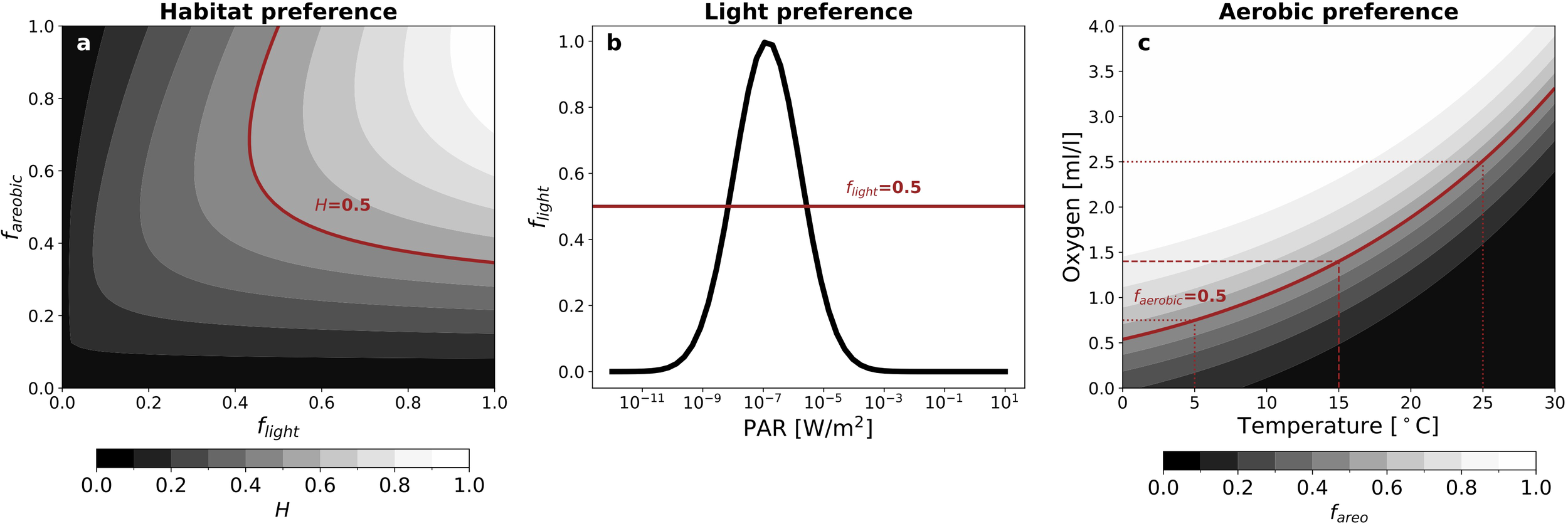
Habitat preferences for the mesopelagic migrant community. (a) Habitat preference, H, as a function of light and aerobic preferences (Equation 4). (b) Light preference, flight, for the migratory community with calibrated parameter values s = 0.1 [W/m2], m = 0.004 [W/m2], for a 12-hour day (Equation 5). (c) Aerobic preference, fareobic, for the migratory community as a function of temperature and oxygen with calibrated parameter values [ml ] and [(ml ] (Equations 6, 7). Red lines mark values of 0.5 (out of 1) for each preference variable as a reference.
where ϕ, T, O represent irradiance [W m−2], temperature [K] and oxygen concentration [ml l−1] respectively.
The light preference, flight [non-dimensional], captures the behavior of mesopelagic organisms to seek dimly lit waters during the daytime to hide from predators (Maury, 2010; Belharet et al., 2024). The light preference peaks in waters that are just dark enough to suppress visual predation and leads the migrating community to dive from the epipelagic zone into the mesopelagic zone during the day (Figure 1b). It is calculated as
where and . The tunable parameters m [W m−2] and s [W m−2] set the mean and variance of the flight distribution. is the irradiance profile with adjustments for length of day and assumed eye allometry.
The aerobic preference, faerobic, reflects the organism’s oxygen demand. In this study, we activate the dependence of metabolic oxygen demand on temperature based on Clarke and Johnston (1999) (Figure 1c).
is a temperature dependent hypoxic threshold that scales with temperature T through an Arrhenius transformation (see Figure 1c for a depiction of how faerobic varies as a function of temperature and oxygen). We use an Arrhenius temperature of Ta = 5020K, which captures the scaling of metabolic rates at a community level (Clarke and Johnston, 1999; Maury et al., 2007) and is similar to values used in previous studies (e.g., Dueri et al., 2012; Aumont et al., 2018). We use a reference temperature of Tref = 288.15K (or 15°C). [ml l−1] and a [(ml l−1)−1] are tunable parameters that set the half-saturation and slope of the oxygen preference when T = Tref. faerobic is also applied as an exponential weight factor such that light preference is only considered when aerobic needs are met (Figure 1a). That is, an individual must be able to breathe in order to pursue preferential light conditions. In this study, we apply the model to communities of small fish. However, the Arrhenius temperature scaling used in the model also describes other members of marine communities, such as zooplankton (e.g. Alcaraz et al., 2013; Packard and Gómez, 2008). We note that there are also other sources of temperature-dependence for fish oxygen needs not accounted for in our model, such as blood oxygen binding affinity (Mislan et al., 2016).
2.2 Earth system model simulations and observations
In this study, we apply the APECOSM-1D ecosystem model to ocean dissolved oxygen and temperature fields from the World Ocean Atlas 2023 and an ensemble of 13 Earth System Models from the Coupled Model Intercomparison Project Phase 6 which provide monthly oxygen, temperature and chlorophyll data for the historical and SSP5-8.5 experiments (CMIP6; Table 1). The relevant output was also available for an additional model, IPSL-CM6A-LL, but was not included in the analysis due to the model’s significant oxygen biases in the tropical Pacific (See diagnostics for areal extent of tropical Pacific OMZ in Supplementary Figure S1; also see e.g., Busecke et al., 2019). We use one member of the historical and SSP5-8.5 high emissions scenario simulations for each Earth System Model. We define ‘present day’ estimates as the monthly climatology between 2004–2022 in the CMIP6 ensemble to compare with the World Ocean Atlas 2023 (WOA23; Garcia et al., 2024; Locarnini et al., 2023). We contrast present day conditions with ‘end of century’ projections, defined as the monthly climatology between 2080–2100 in the SSP5-8.5 simulations. Results for WOA23-based present-day and end-of-century migration depths are computed with monthly climatologies in order to account for seasonal changes in environmental conditions, but all results are presented as annual averages for each case.
Table 1
| Product | Reference |
|---|---|
| World Ocean Atlas 2023 | Locarnini et al. (2023); Garcia et al. (2024) |
| ACCESS-ESM1-5 | Ziehn et al. (2019a, b) |
| CNRM-ESM2-1 | Seferian (2018, 2019) |
| CanESM5 | Swart et al. (2019c, d) |
| CanESM5-CanOE | Swart et al. (2019a, b) |
| GFDL-CM4 | Guo et al. (2018a, b) |
| GFDL-ESM4 | Krasting et al. (2018); John et al. (2018) |
| MIROC-ES2L | Hajima et al. (2019); Tachiiri et al. (2019) |
| MPI-ESM1-2-HR | Jungclaus et al. (2019); Schupfner et al. (2019) |
| MPI-ESM1-2-LR | Wieners et al. (2019a, b) |
| MRI-ESM2-0 | Yukimoto et al. (2019a, b) |
| NorESM2-LM | Seland et al. (2019a, b) |
| NorESM2-MM | Bentsen et al. (2019a, b) |
| UKESM1-0-LL | Tang et al. (2019); Good et al. (2019) |
Earth system models from CMIP6 experiments.
Observation-based products and Earth system models used in this study. For all Earth System Models, we use oxygen, temperature, shortwave radiation, and chlorophyll fields for a single member. All Earth system model outputs used are publicly available via the Earth System Grid Federation.
Depth-resolved irradiance fields are calculated from monthly surface short-wave radiation and depth-resolved chlorophyll fields in the CMIP6 ensemble for historical and SSP5-8.5 simulations using the absorption algorithm described in Lengaigne et al. (2007). When applying APECOSM-1D to the World Ocean Atlas, we use depth-resolved irradiance fields from a hindcast simulation using the physical biogeochemical model NEMO-PISCES (Aumont et al., 2015), which is forced by atmospheric conditions from JRA-55 (Kobayashi et al., 2015) and also employs the absorption algorithm from Lengaigne et al. (2007). We use a monthly climatology between 2004–2022 from the NEMO-PISCES hindcast simulation.
In addition to computing migration depths based on present-day and end-of-century ocean conditions, we also perform a suite of sensitivity tests where only one ocean field (oxygen, temperature or irradiance) is changed at a time. We interpret these single-variable experiments to determine the relative influences of projected oxygen, temperature and light changes on migration depths.
2.3 Tuning APECOSM-1D model parameters
We calibrate the light and aerobic preference parameters in the APECOSM-1D model against processed low-frequency (38 kHz) acoustic sounding profiles from the Malaspina 2010 circumnavigation (Duarte, 2015; Irigoien et al., 2020; Ariza et al., 2022). These observed profiles provide an estimate of the vertical distribution of biomass in the upper 1000 m of the ocean. While the composition of the migrating mesopelagic communities was not fully assessed in-situ during the Malaspina expedition, the backscatter in this dataset is assumed to be dominated by the gas-filled swim bladders of myctophids and species of the Cyclothone genus (i.e., small fish of length on the order of 10 cm; Irigoien et al., 2014). Earlier studies suggest that crustaceans, euphausiids and siphonophores likely also make up part of the signal (Moore, 1950; Barham, 1966). In this study, though, we effectively model the observed signal as a monolithic migrating community of fish with a body length of 10 cm.
For calibration, we use the monthly climatology of dissolved oxygen and temperature from the World Ocean Atlas 2023, along with monthly-mean irradiance profiles from the NEMO-PISCES hindcast simulation corresponding to the month of each observed profile. We configure the model to represent three communities simultaneously: epipelagic, mesopelagic resident and mesopelagic migrant, in order to account for all the biomass components that are present in reality and reflected in the data. Each community is associated with an independent set of model parameter values to reflect different behaviors and preferences (Supplementary Table S1): The epipelagic community is characterized by a bright light preference, while mesopelagic residents and migrants are characterized by dimmer light preferences. The mesopelagic resident and migrant communities differ in that the resident communities maintain the daytime depth at night while migrants swim up to epipelagic depths at night. By comparing the daytime and nighttime data from the acoustic sounding profiles, we infer the relative biomasses of each community and apply that partitioning to a weighted sum of the three modeled community profiles.
We use the differential_evolution optimization scheme from the scipy.optimize package with a simple root-mean-square cost function for daytime biomass profiles. Light preference parameters (m, s) for the migrating community were tuned using sounding profiles in well-oxygenated regions (‘General Pattern’ profiles in Belharet et al. (2024); red profiles in Figure 2). Parameters for aerobic preference (a and in Equations 6, 7) were tuned using sounding profiles over the eastern tropical Pacific oxygen minimum zone (‘Shallow Pattern’ profiles in Belharet et al. (2024); blue profiles in Figure 2). See Supplementary Table S1 for the full set of model parameter values.
Figure 2
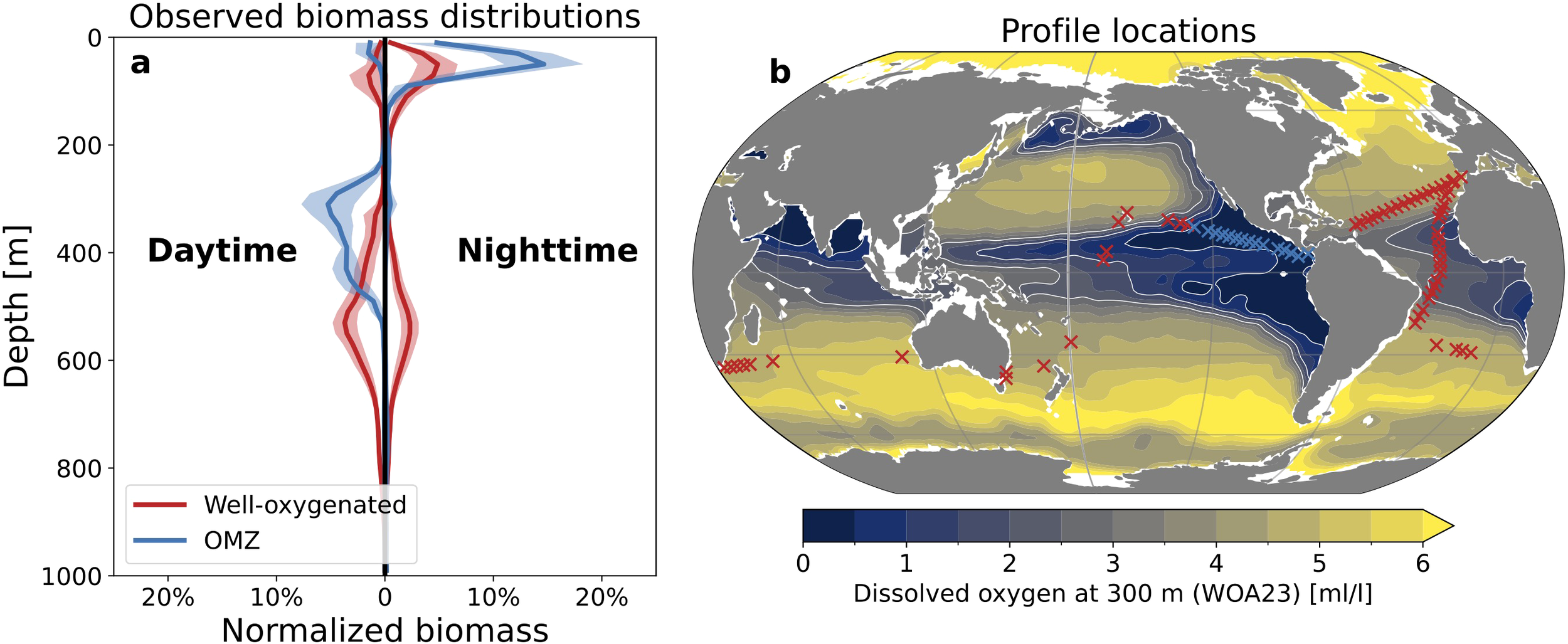
Observed vertical biomass distributions. (a) Relative biomass distributions based on Malaspina 2010 acoustic sounding profiles over well-oxygenated regions (red) and the Pacific Ocean oxygen minimum zone (OMZ; blue). Solid curves are sample mean and shading is one standard deviation. (b) Locations of well-oxygenated and OMZ sample points compared with dissolved oxygen at 300 m from the World Ocean Atlas 2023 (WOA23). Thin white contours highlight 0.5, 1.5 and 2.5 ml/l oxygen.
3 Results
3.1 Reproducing acoustic observations
Both the vertical distribution of biomass and the community composition over OMZs differ from well-oxygenated regions (Figure 2). In well-oxygenated regions, observed biomass distributions are characterized by an epipelagic resident community (0–200 m), a mesopelagic resident community (200–800 m), and a migrating community that is observed at mesopelagic depths during the day and epipelagic depths at night (red curves in Figure 2a). In both daytime and nighttime profiles, mesopelagic biomass peaks between 500 and 600 m depth in well-oxygenated regions. The samples that make up this characteristic profile are largely collected from the well-oxygenated Atlantic Ocean, but also include samples from well-oxygenated regions in the Pacific and Southern Indian Oceans (red x’s in Figure 2b). Belharet et al. (2024) suggest that migration depths in well-oxygenated waters are likely determined by light levels such that species avoid visual predation. In contrast, observations over the Pacific Ocean OMZ (blue x’s in Figure 2b) exhibit a daytime peak in mesopelagic biomass between 200 and 500 m, with little-to-no mesopelagic biomass at night (blue curves in Figure 2a). While resident communities dominate the mesopelagic biomass in well oxygenated regions, the OMZ acts as a habitat barrier which excludes mesopelagic resident communities. In turn, the daytime mesopelagic biomass in the OMZ is composed almost entirely by the migrating community. Furthermore, the OMZ forces shallower migration depths compared to well-oxygenated regions.
The calibrated model captures the daytime and nighttime distribution of mesopelagic and epipelagic biomass in well-oxygenated waters and over the tropical Pacific OMZ (Figures 3a, b). In well-oxygenated waters, the modeled migratory community exhibits mean daytime dive depths of about 470 m and contribute primarily to the shallower tail of the daytime mesopelagic biomass (Figure 3a; migratory community represented by purple dashed curves). Over the OMZ, the modeled migratory community exhibits shallower mean daytime dive depths of about 330 m and compose virtually all of the daytime mesopelagic biomass (Figure 3b). In the model, migration depths in well-oxygenated waters are primarily determined by light, while migration depths over the OMZ are primarily determined by oxygen and the temperature-dependent oxygen demand of metabolism (See Methods; scaling of aerobic preference with temperature shown in Figure 1c): in warmer waters, metabolic rates increase resulting in greater oxygen demand. In the calibrated model at a reference temperature of 15°C, the threshold for hypoxia (defined here as an aerobic preference of 0.5 on a scale of 0 to 1) is about 1.4 ml/l. For ambient temperatures of 5°C and 25°C the modeled hypoxic threshold shifts to 0.75 ml/l and 2.5 ml/l, respectively. In turn, a warmer OMZ is likely to act as a stronger habitat barrier compared to a colder OMZ with the same oxygen concentration. Since temperature decreases with depth, a shallower OMZ is likely to act as a stronger habitat barrier compared to a deeper OMZ. That is, the criteria for hypoxia will be more easily satisfied closer to the surface.
Figure 3
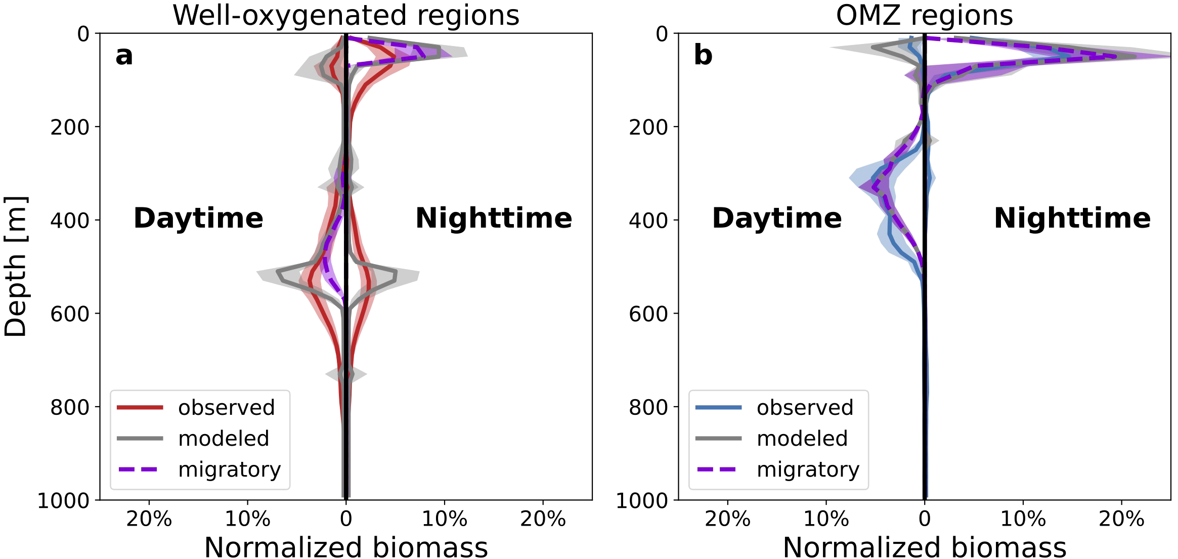
Model of vertical biomass and migration depths. (a) Observed (red) and modeled (gray) daytime and nighttime relative biomass distributions in well-oxygenated regions. (b) Observed (blue) and modeled (gray) daytime and nighttime relative biomass distributions over the Pacific Ocean oxygen minimum zone (OMZ). Solid curves are sample mean and shading is one standard deviation. Purple dashed curves and shading are the component of modeled biomass from the migratory community.
3.2 Reconstructing migration depths from the World Ocean Atlas and CMIP6 ensemble
Using the calibrated one-dimensional ecosystem model, we reconstruct mean migration depths over the tropical Pacific Ocean OMZ in the World Ocean Atlas 2023 (WOA23) climatology and in present-day simulations from CMIP6 Earth System Models (Figure 4). In the WOA23-based reconstruction, mean migration depths are hundreds of meters shallower over the OMZ core than over the subtropical gyres where mean migration depths reach 400 m. Over the OMZ, about 19 × 106 km2 exhibit mean migration depths shallower than 200 m (dark blue contours in Figure 4a). The ensemble mean reconstruction from CMIP6 also captures the shallower migration depths over the OMZ compared to the subtropical gyres (Figure 4b). In the ensemble mean reconstruction, about 14 × 106 km2 exhibit mean migration depths shallower than 200 m (dark blue contours in Figure 4b). This underestimation of the areal extent of shallow migration depths (compared to the WOA23-based reconstruction) stems from a failure to capture the western extent of the OMZ. This is partially due to systematic biases across the CMIP6 ensemble resulting from poorly resolved equatorial circulation (see results for individual Earth System Models in Supplementary Figure S2; Montes et al., 2014; Busecke et al., 2019).
Figure 4
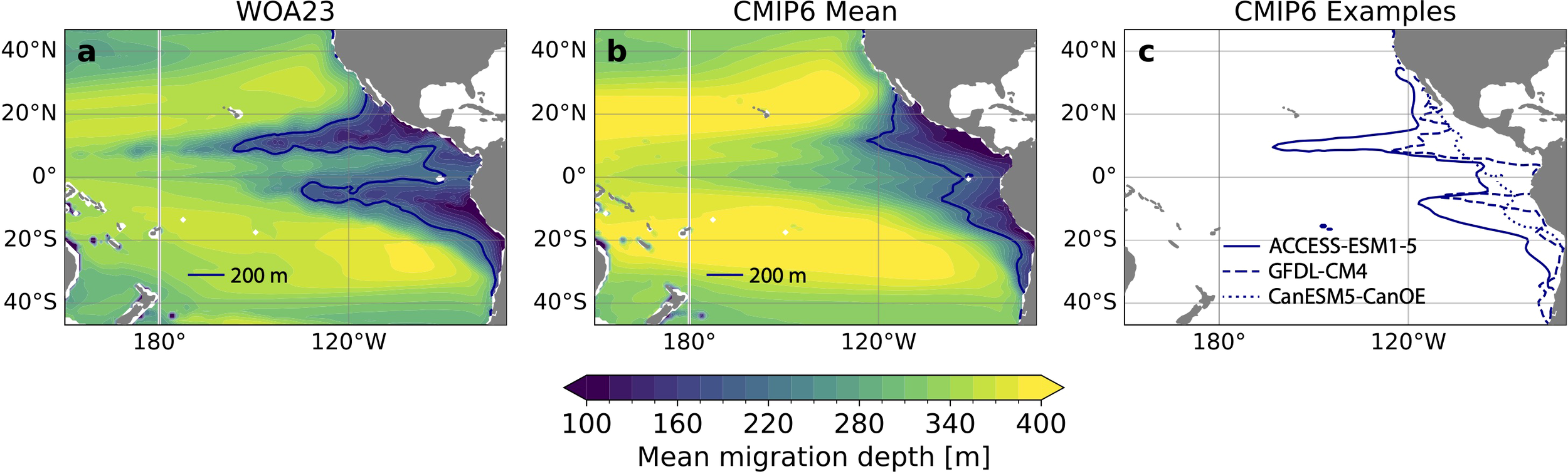
Modeled migration depth patterns based on observations and simulations. (a) Daytime weighted mean vertical migration depths based on oxygen and temperature from the World Ocean Atlas 2023 (WOA23). (b) Multi-model mean of daytime weighted mean vertical migration depths based on oxygen and temperature from present-day CMIP6 simulations. 200 m migration depth contours (dark blue) are highlighted. (c) 200 m migration depth contours for three example Earth System Models from the CMIP6 ensemble (ACCESS-ESM1-5, GFDL-CM4, CanESM5-CanOE) illustrating the range of OMZ representations across the ensemble.
Despite systematic biases across the CMIP6 ensemble, many models represent the spatial structure of the western extent and/or the equatorial structure of the OMZ (Supplementary Figure S2). However, spatial structure in these models is damped in the composite map due to misalignment of features across the ensemble. Figure 4c demonstrates the variability in OMZ representations with three examples from the CMIP6 ensemble as reflected by the 200 m mean migration depth contour. In ACCESS-ESM1-5 (solid contours in Figure 4c), the western extent of the OMZ is similar to WOA23, with 200 m migration depth contours reaching about 170°W in the north and 120°W in the south. However, this model also overestimates the OMZ presence around the equator. In contrast, GFDL-CM4 (dashed contours) somewhat underestimates the western extent of the OMZ, but better captures the equatorial separation of the OMZ lobes. Finally, CanESM5-CanOE simulates an OMZ that is trapped close to the eastern boundary with virtually no equatorial separation. The composite map of migration depths in the CMIP6 ensemble (Figure 4b) thus aggregates different dynamical regimes across the model ensemble at a given location.
Figure 5 further illustrates the patterns of migration depths over the OMZ as reconstructed based on WOA23 and the CMIP6 ensemble present-day simulations. WOA23-based migration depths exhibit distinct meridional and zonal structure related to the OMZ cores (white lines; Figures 5a–c). Meridionally, migration depths are shallowest over the OMZ cores and deepen around the equator (Figure 5a). Zonally at 12°N and 10°S, migration depths are shallowest at the eastern boundary over the OMZ cores, and gradually deepen westward (Figures 5b, c). The ensemble mean CMIP6-based reconstruction captures these general patterns, with shallowest migration depths off the equator and along the eastern boundary (shaded cyan lines; Figures 5a–c). However, the ensemble mean CMIP6-based reconstruction underestimates the contrast between the equatorial region and off-equatorial OMZ cores, resulting in migration depths too shallow at the equator and too deep over the OMZ cores (Figures 5a–c). As seen in Figure 4, some of this bias is due to the smoothing of features when averaging across the ensemble. So, we also highlight the reconstructed migration depths in the three example individual models shown in Figure 4c.
Figure 5
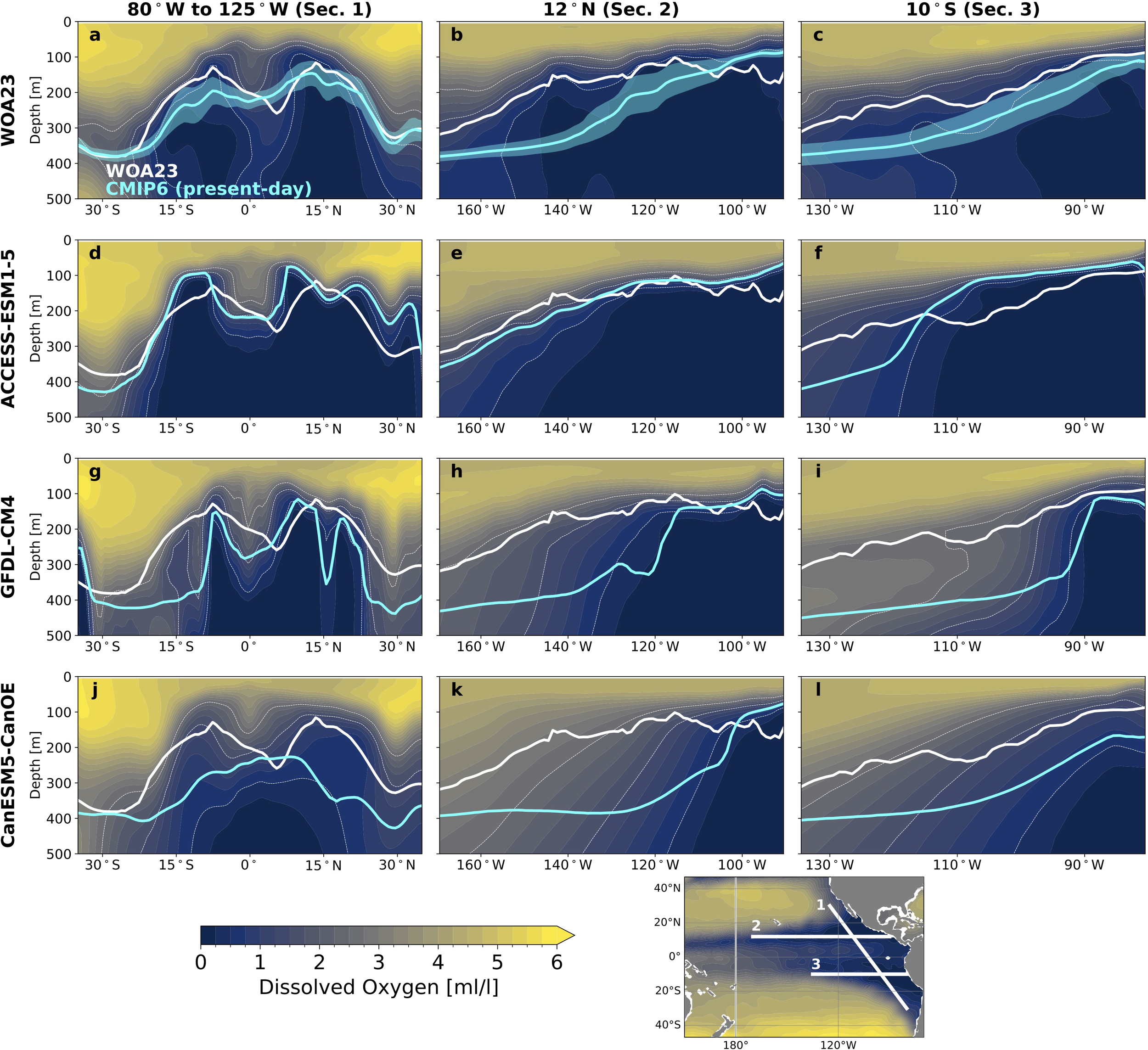
Migration depths over the oxygen minimum zone. (a–c) Sections of oxygen concentrations in the World Ocean Atlas 2023 (WOA23; color), WOA23-based mean migration depth (white line) and CMIP6 present-day ensemble-mean mean migration depth (cyan line; shading is one standard deviation across ensemble) (a) along the eastern boundary and along (b) 12°N and (c) 10°S. (d–f) Sections of present-day oxygen concentrations in ACCESS-ESM1–5 and model-based mean migration depths for ACCESS-ESM1-5 (cyan) (d) along the eastern boundary and along (e) 12°N and (f) 10°S. (g-i) Same as d-f for GFDL-CM4. (j–l) Same as (d–f) for CanESM5-CanOE. WOA23-based migration depths added to panels (d–l) (white) for comparison. Thin white dashed contours highlight 0.5, 1.5 and 2.5 ml/l oxygen. The section locations are shown in white on the map in lower right.
Migration depths reconstructed from ACCESS-ESM1–5 agree well with the WOA23-based reconstruction, with shallow migration depths over the OMZ cores and deeper migration depths over the equator (Figures 5d–f); however, the southern OMZ core is more intense than in WOA23, resulting in a shallow-bias of migration depths. In contrast, migration depths reconstructed from GFDL-CM4 and CanESM5-CanOE tend to be biased deep compared to WOA23, with some exceptions near the equator (Figures 5g–l). Overall, a deep bias in migration depths over the OMZ will likely underestimate simulated sensitivity to temperature effects on hypoxic tolerance, which are strongest closer to the surface. Conversely, shallow-biased migration depths over the equator– and more broadly in models like ACCESS-ESM1-5– may be overly sensitive to temperature effects on hypoxic tolerance.
3.3 Projected migration depth changes from oxygen, temperature and light changes
In individual models, reconstructed migration depths can shift dramatically between present-day and SSP5-8.5 end-of-century conditions. Figure 6 shows present-day (cyan) and end-of-century (magenta) migration depths in relation to projected changes in dissolved oxygen (panels a-c) and temperature (panels d-f) for our three example models (the effects of projected light changes are also shown in Supplementary Figures S3–S5). In ACCESS-ESM1-5, changing conditions deepen migration depths into the OMZ cores and shoal migration depths over the equator (Figure 6a). The end-of-century migration depths closely match the migration depths estimated by oxygen changes alone (dashed magenta lines in Figure 6a). A similar pattern emerges for projected changes from GFDL-CM4, though milder deoxygenation around the equator results in a weaker shoaling compared to that from ACCESS-ESM1-5 (Figure 6b). This suggest that the pattern of change is primarily dictated by oxygen changes, while temperature changes modulate the magnitude of the effect. In contrast, projected migration depths from CanESM5-CanOE– in which the OMZ core spans the equator– exhibit more widespread shoaling between 15°S and 15°N, and only about half of the shoaling is accounted for by oxygen-driven changes alone. Indeed, temperature-driven migration depth changes are stronger in CanESM5-CanOE compared to ACCESS-ESM1–5 and GFDL-CM4 (dotted magenta lines in Figures 6d–f). For both ACCESS-ESM1–5 and GFDL-CM4, projected warming drives mild but consistent shoaling, whereas warming drives significant shoaling in the CanESM5-CanOE-based reconstruction. Along zonal sections at 12°N and 10°S, oxygen anomalies dominate and drive a deepening of migration depths in ACCESS-ESM1–5 and GFDL-CM4, but temperature changes dominate and drive shoaling in CanESM5-CanOE (Supplementary Figures S3–S5). For all three models, changes in light availability have only a small effect on migration depths over the OMZ (Supplementary Figures S3–S5).
Figure 6
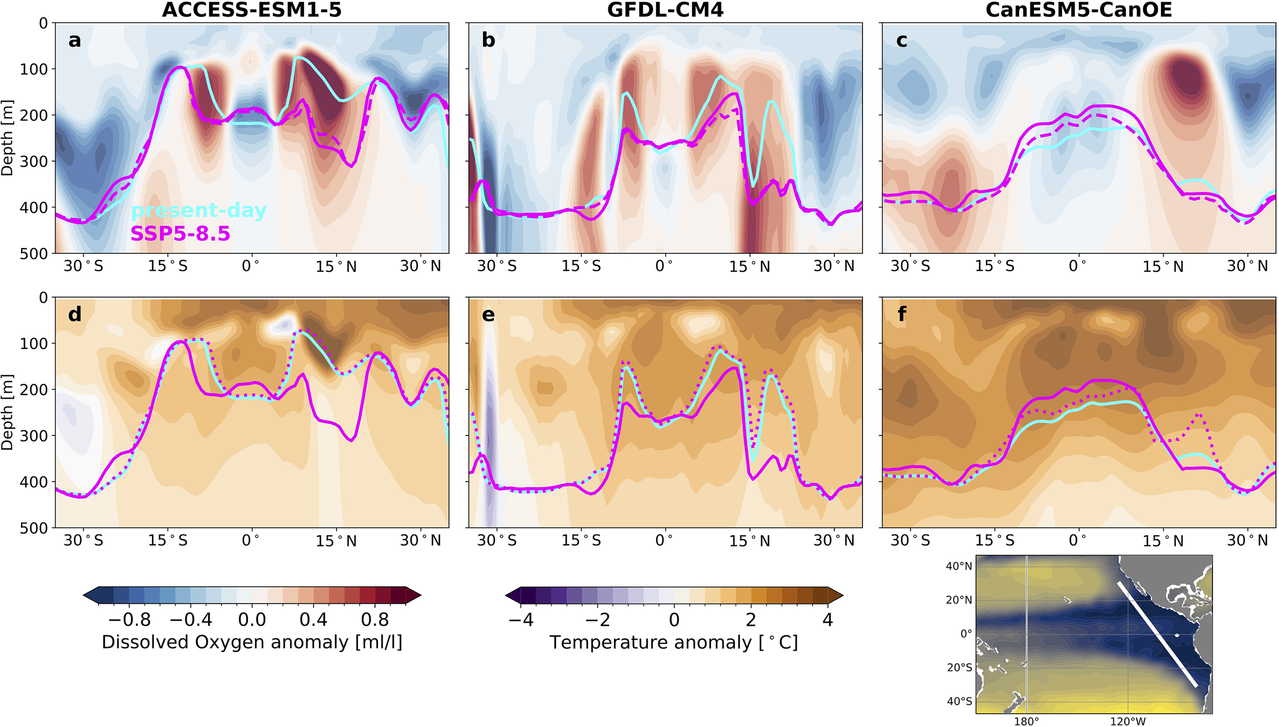
Changes in migration depths over the oxygen minimum zone and contributions from oxygen and temperature changes. Sections along the eastern boundary (location shown in lower right panel) of (a–c) dissolved oxygen anomalies and (d–f) temperature anomalies (SSP5-8.5 end-of-century minus present-day). Results are shown for (a, d) ACCESS-ESM1-5, (b, e) GFDL-CM4, and (c, f) CanESM5-CanOE. Reconstructed migration depths are shown for: present day (cyan), end-of-century (solid magenta), end-of-century expected from oxygen changes only (dashed magenta in a–c), end-of-century expected from temperature changes only (dotted magenta in d–f).
In ensemble mean composite geographic sections, the strong changes found in individual models largely get smoothed out (Supplementary Figure S6), and reveal a systematic compensation between oxygen-driven deepening and temperature-driven shoaling over much of the sections. In the next section we present an approach to dynamically isolate features across the ensemble in order to generalize the patterns we find in individual models.
3.3.1 Isolating migration depth changes by oxygen minimum zone region
To align similar features across the CMIP6 ensemble, we define regions of the OMZ using the present-day minimum of the vertical oxygen concentration in the upper 400 m of the ocean in each model, which also correlates well with the depth of the oxycline (Supplementary Figure S7). We bin the OMZ into five regions: one core region (oxygen minima from 0 to 0.5 ml/l), two intermediate regions (oxygen minima from 0.5 to 1.0 ml/l and 1.0 to 1.5 ml/l), and two outer regions (oxygen minima from 1.5 to 2.0 ml/l and 2.0 to 2.5 ml/l; see colored guides in Figure 7). Migration depths deepen or shoal by as much as 200 m in some locations (see black violin plots in Figure 7c; spines of violin plots span the central 98% of area over each region of the OMZ). For instance, over the OMZ core, migration depths deepen by up to 200 m and shoal by up to 100 m in some locations (Figure 7c; Supplementary Figure S8). In the first intermediate OMZ region (oxygen minima from 0.5 to 1.0 ml/l), migration depth projections exhibit the widest range with shoaling up to 200 m and deepening up to 150 m. For OMZ regions with oxygen minima greater than 1 ml/l, the range of migration projections decreases as the oxygen minima increases.
Figure 7
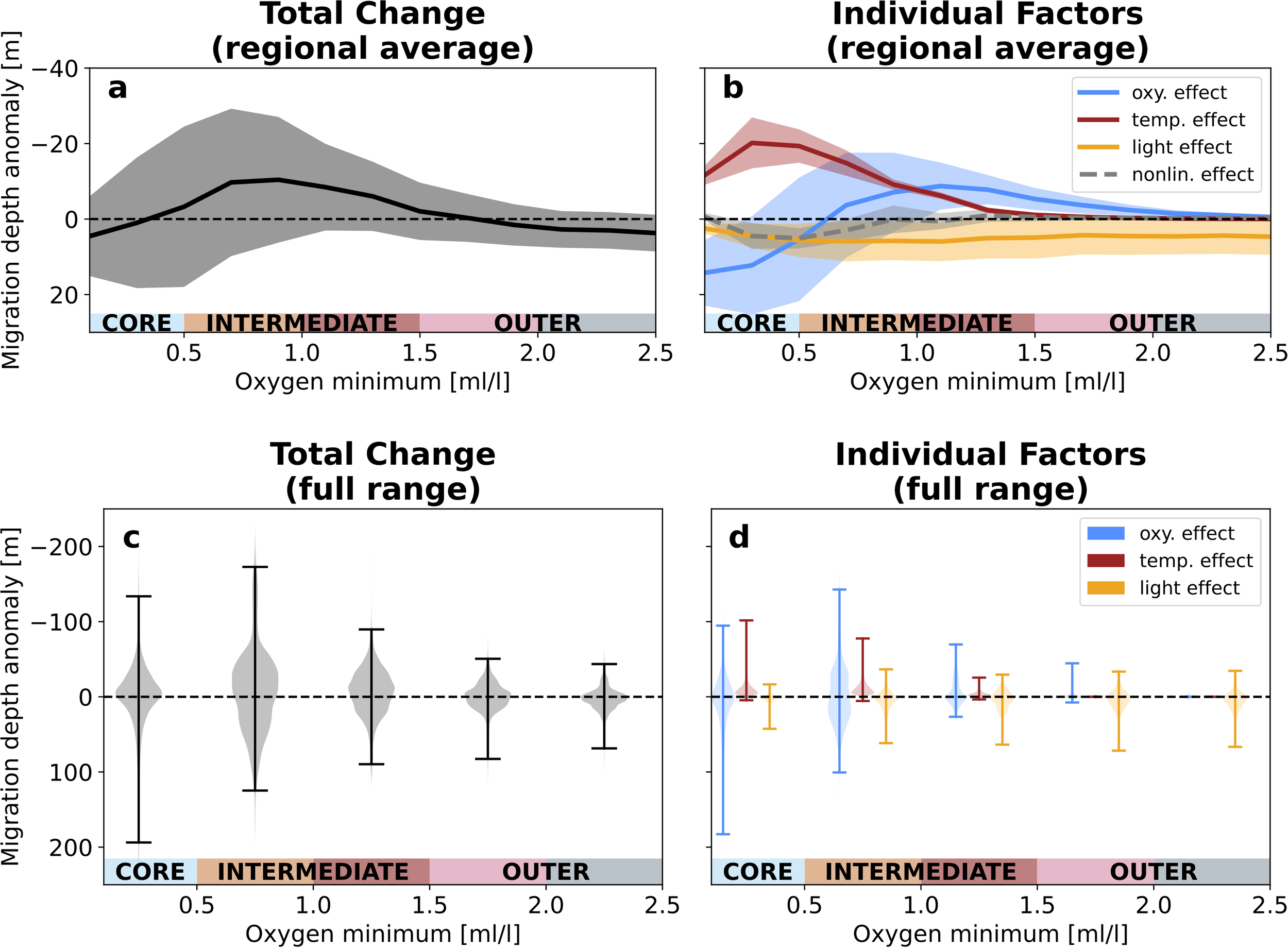
Drivers of change by oxygen minimum zone region. (a) Regional average total migration depth anomalies (SSP5-8.5 end-of-century minus present-day) and (b) regional average anomalies due to changes in oxygen (blue), temperature (red) and light (orange) as a function of oxygen minimum concentration in the upper 400 m. Solid curves are the CMIP6 ensemble mean of regional average anomalies and shading is one standard deviation across the CMIP6 ensemble. (c) Violin plots showing the distribution of daytime migration depth anomalies aggregated by OMZ region. (d) Violin plots showing the distribution of migration depth anomalies due to changes in oxygen (blue), temperature (red) and light (orange). Each violin is the CMIP6 ensemble mean of the kernel-density estimate distributions calculated for each model. Spines span the central 98% of the distribution.
As described above, migration depths are projected to shoal in some locations and deepen in others for all regions of the OMZ (core, intermediate, outer regions). In turn, the dramatic local migration depth changes largely compensate when averaged over each OMZ region. Here, we assess the change in migration depths on average in each of these OMZ regions. Figure 7a shows the ensemble results for mean changes across models as a function of present-day oxygen minimum concentration in the upper 400 m (ensemble mean and one standard deviation across the ensemble of model mean changes). The ensemble mean changes are within one standard deviation of zero change across the spectrum of OMZ layers due to spatial compensation between shoaling and deepening (Figure 7c), but do exhibit a clear structure across regions. On average, migration depths weakly deepen over the OMZ core, shoal over intermediate regions, and exhibit weak deepening over outer regions (Figure 7a). Figure 7b shows the mean effects of changes in each individual factor (oxygen in blue, temperature in red, and light in orange; full range of local effects in each region are shown in Figure 7d), as well as nonlinear interactions between factors (gray dashed line, calculated as a residual). Migration depth changes over the OMZ core are characterized by a compensation from changes in oxygen and temperature. The OMZ core experiences strong oxygenation over the century, but the shallow migration depths over the OMZ core expose mesopelagic migrants to a pronounced near-surface warming, which increases their oxygen needs (Figure 6). Over the intermediate OMZ layers, deoxygenation and warming compound to drive an ensemble mean shoaling of migration depths. Over the outer OMZ layers, the effects of deoxygenation and increased irradiance at depth (due to projected decline in tropical primary production and chlorophyll; see e.g., Bopp et al., 2013; Kwiatkowski et al., 2020) offset each other, while temperature has virtually no effect on migration depth changes. Between 1.5 and 2 ml/l, compensating oxygen and light changes lead to near zero average migration depth changes. Between 2 and 2.5 ml/l, aerobic constraints are weak and migration depths deepen with increased irradiance.
The aggregation of migration depth projections over layers of the OMZ serves two purposes: (1) we troubleshoot the spatial mismatches of features across the model ensemble and (2) we can better relate projected changes to observed present day conditions. By isolating changes over each OMZ layer in the CMIP6 ensemble, we can infer where migration depth changes are likely to occur in the real ocean. We now compare the patterns of change from the CMIP6 ensemble (Figure 7) to the geographic distribution of OMZ layers based on WOA23 (Figure 8a). The average pattern of change in each OMZ region is depicted schematically in Figure 8b. The CMIP6 ensemble suggests that changes to migration depths over the observed OMZ core region, shaded in blue, will be characterized by a compensation of effects from increased oxygen and near-surface warming. Migration depths over the intermediate OMZ layers shaded in orange and red will likely shoal from a combination of deoxygenation and surface warming. Finally, migration depths over the outer layers of the OMZ shaded in pink and gray will likely be only weakly affected by deoxygenation and unaffected by warming.
Figure 8
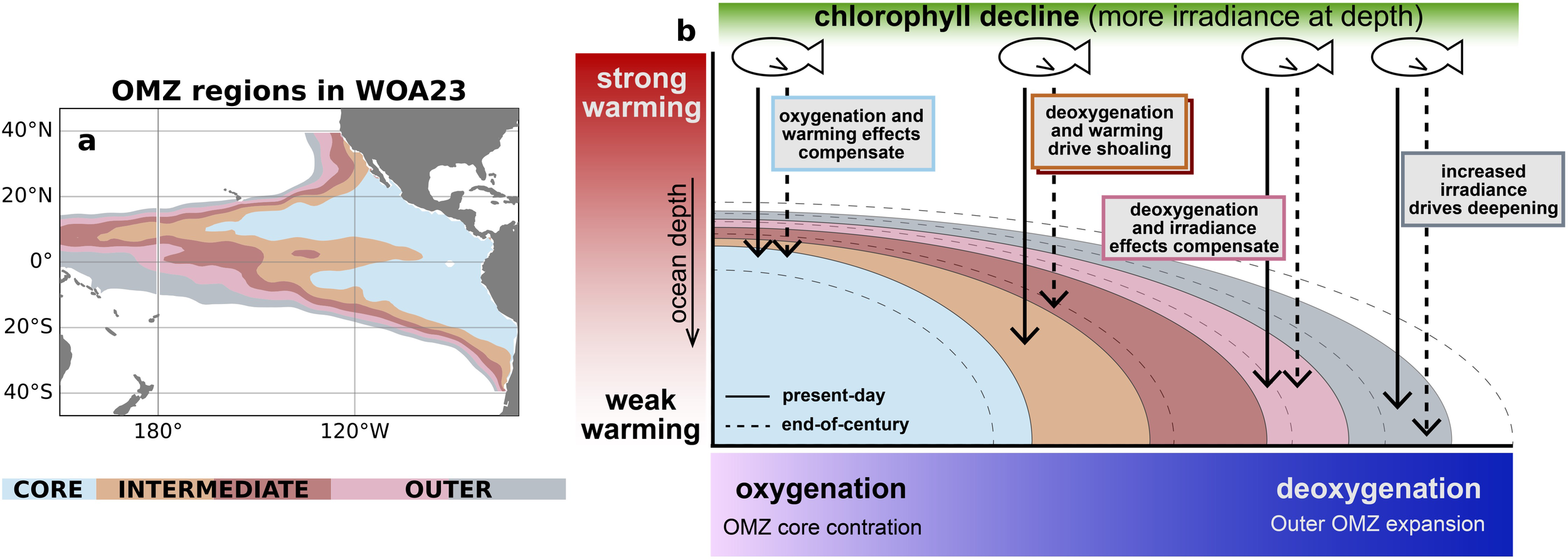
Schematic of migration depth changes. (a) Map of oxygen minimum zone regions from World Ocean Atlas 2023 (WOA23). (b) Schematic summary of CMIP6-based ocean and migration depth changes averaged over each OMZ region.
4 Discussion
We implemented a temperature-dependent representation of hypoxia tolerance in a simplified ecosystem model (APECOSM-1D) to assess future changes in diel vertical migration depths across the eastern tropical Pacific oxygen minimum zone (OMZ). The computational efficiency of the APECOSM-1D implementation allowed us to perform a suite of sensitivity tests to determine the role of individual environmental conditions (dissolved oxygen, temperature and light) on migration depth changes based on an ensemble of 13 climate models from CMIP6. We find that projected changes in migration depth generally reflect the pattern of OMZ projections in the CMIP6 ensemble, in which OMZ cores tend to contract with warming while the outer layers of the OMZ expand (Gnanadesikan et al., 2012; Busecke et al., 2022; Ditkovsky et al., 2023). Over the core regions of the OMZ where present-day hypoxia is most intense, we find that the degradation of aerobic habitat suitability caused by ocean warming will likely be compensated on average by increased dissolved oxygen levels, resulting in little change in migration depths. The OMZ core generally coincides with the shallowest oxycline depths, and thus will be where the quality of aerobic habitats are most sensitive to ocean warming. Furthermore, the influence of ocean warming is likely underestimated in the results here because OMZs, and in turn oxycline depths, in the CMIP6 ensemble tend to be deeper than in observations. Away from the OMZ core, specifically over intermediate OMZ layers, ocean warming and deoxygenation compound on average to degrade aerobic habitats, resulting in shallower migration depths in the future.
Regional mean changes in migration depth have implications for future changes in the strength of the biological carbon pump (Bianchi et al., 2013b): overall shallower migration patterns will likely weaken the export rates of carbon by migrating communities (Nowicki et al., 2022). While zooplankton are thought to dominate the “migrant pump”, the size class of fish modeled here (order 10 cm) may also provide significant contributions (Saba et al., 2021). Additionally, the APECOSM model can also be applied to size classes which encompass much of the zooplankton community (order 1 mm; Lefort et al., 2015), and would likely yield similar responses to environmental changes. Furthermore, the models analyzed in this study suggest that at a given location over the OMZ, migration depths may shoal or deepen by over 100 m. These local changes in migration depth could impose significant perturbations to predator-prey dynamics by changing the availability of mesopelagic prey to epipelagic predators (Dini and Carpenter, 1992; Pinti et al., 2019; Bertrand et al., 2004). While assessing changes in the overall biomass of each community (epipelagic, mesopelagic residents, and mesopelagic migrants) is beyond the scope of this study, such changes are also possible in response to environmental changes and could perturb both the biological carbon pump and predator-prey dynamics. Specifically, observations (e.g., Figure 2) and laboratory experiments (Vaquer-Sunyer and Duarte, 2008) suggest that in the present climate, mesopelagic residents are largely excluded from the core of OMZs. Future oxygenation of the OMZ core could thus open up entirely new habitats for mesopelagic residents and change the biomass partitioning between residents and migrants in the Eastern Tropical Pacific.
The simplified APECOSM-1D model used in this study is able to effectively reproduce observed migration depths both over the eastern tropical Pacific OMZ and in well-oxygenated regions. However, it neglects important biological and ecological characteristics that might factor into the response of vertical migrations to changes in hypoxia. Specifically, while the metabolic demand rate for oxygen is strongly related to the body size of organisms and to the size of their species (Clarke and Johnston, 1999; Kooijman, 2010), the capacity to extract oxygen from water and supply it to organs also scales with size, but in a potentially different way, thus leading to a possible size-dependence of the hypoxia tolerance (i.e. the critical oxygen concentration level below which demand exceeds supply). However, both oxygen demand and supply also vary with the species considered, individual activity, condition, maturity, and behavioral mode, thus leading to complex links between size and oxygen limitation and fuzzy relationships in observations (e.g., Verberk et al., 2022), the conclusions of which are still being actively debated (e.g., Lefevre et al., 2017; Pauly, 2021). Given this lack of scientific consensus, and while awaiting a convincing formal theory to explain the complexity and variability of oxygen limitation, the critical oxygen concentration below which fishes suffer from hypoxia is held constant (but community- and temperature-dependent) in this study. In the future, a more sophisticated physiology-based model representation of hypoxia tolerance might allow to extend our conclusions to explain size-dependent oxygen limitation such as shown in Salvatteci et al. (2022), who find that the size composition of communities in the eastern tropical Pacific may have shifted significantly in conjunction with climate changes over the last 100 thousand years. Other aspects of ecosystem dynamics neglected in this study include the role of food in shaping the vertical distribution of fish, which is treated in the full 3D APECOSM (e.g., Dalaut et al., 2025). Also, feedback between vertically migrating communities and the underlying ocean conditions might play an important role. Indeed, some studies suggest that oxygen consumption by higher trophic level communities could represent a significant oxygen sink at the top of OMZs (Bianchi et al., 2013a; Jennings et al., 2008). However, this is still uncertain as subsequent evidence suggests that the contribution of higher trophic level oxygen consumption in OMZs may be more marginal than previously thought due to compensation by passive fluxes and the suppression of metabolic activity in hypoxic environments (Aumont et al., 2018; Kiko and Hauss, 2019).
Climate models are powerful tools for understanding and projecting ecosystem behavior, but care must be taken in their application and interpretation. Here, we take a tailored, computationally efficient approach designed to gain a mechanistic understanding of potential migration depth changes over the OMZ. This study complements and informs much larger-scale efforts to leverage ocean, climate and ecosystem models, such as the Fisheries and Marine Ecosystem Model Intercomparison Project (FishMIP) (Novaglio et al., 2024; Blanchard et al., 2024). The present study highlights the importance of understanding the underlying climate model projections of ocean water masses before extrapolating ecosystem impacts. For example, we demonstrate that relevant features may not align geographically across the model ensemble and observations, but that feature-specific information can be leveraged across the model ensemble and extrapolated to the real ocean. Ocean features, including OMZs, are often misaligned across model representations and observations (Busecke et al., 2022). However, in many cases these features can be isolated across models with frameworks based on water masses (Groeskamp et al., 2019; Iudicone et al., 2011; Ditkovsky and Resplandy, 2024). Here, we define OMZ layers according to minimum oxygen concentrations in order to align ocean features across models and isolate the spectrum of oxygen changes in the core and outer layers. For future work in coupling climate and ecosystem models, characterizing the ways in which ecosystems interact with water masses– rather than how they respond at a fixed geographic location– may yield the most reliable and interpretable signals.
5 Conclusions
We examine the effects of oxygen and temperature as co-evolving stressors in the tropical Pacific Ocean OMZ, with a focus on how future changes may impact diel vertical migration depths. We apply a vertical ecosystem model to CMIP6 high-emission scenario ocean projections to account for depth-resolved changes in habitat suitability. While the CMIP6 ensemble exhibits significant diversity in its ocean projections, and in turn projections of migration depths, all CMIP6 projections suggest that local migration depths may deepen or shoal by over 100 m. When averaged over the core, migration depths are likely to remain stable as the result of compensations between warmer temperatures and more abundant subsurface oxygen. Away from the OMZ core, the experiments suggest that deoxygenation and warming together can drive a shoaling of migration depths. This study suggests that changes in tropical ocean conditions, particularly around OMZs, can impact predator-prey dynamics and the efficiency of the biological carbon pump.
Statements
Data availability statement
The datasets generated and analyzed for this study, as well as software to recreate manuscript figures, can be found at https://zenodo.org/records/17228682.
Author contributions
SD: Conceptualization, Data curation, Formal Analysis, Funding acquisition, Investigation, Methodology, Software, Validation, Visualization, Writing – original draft, Writing – review & editing. LR: Conceptualization, Funding acquisition, Supervision, Writing – original draft, Writing – review & editing. LD: Methodology, Software, Validation, Writing – review & editing. NB: Data curation, Software, Writing – review & editing. ML: Data curation, Methodology, Writing – review & editing. OM: Conceptualization, Investigation, Methodology, Resources, Software, Supervision, Writing – original draft, Writing – review & editing.
Funding
The author(s) declared that financial support was received for this work and/or its publication. SD was supported by the High Meadows Environmental Institute (HMEI) Hack Award for Water and the Environment and LR’s NSF CAREER award no. 2042672 and HMEI Grand Challenge research award. LD was funded by Programme Prioritaire Ocean et Climat (PPR, grant ANR n° 22-POCE-0001).
Conflict of interest
The authors declared that this work was conducted in the absence of any commercial or financial relationships that could be construed as a potential conflict of interest.
Generative AI statement
The author(s) declared that generative AI was not used in the creation of this manuscript.
Any alternative text (alt text) provided alongside figures in this article has been generated by Frontiers with the support of artificial intelligence and reasonable efforts have been made to ensure accuracy, including review by the authors wherever possible. If you identify any issues, please contact us.
Publisher’s note
All claims expressed in this article are solely those of the authors and do not necessarily represent those of their affiliated organizations, or those of the publisher, the editors and the reviewers. Any product that may be evaluated in this article, or claim that may be made by its manufacturer, is not guaranteed or endorsed by the publisher.
Supplementary material
The Supplementary Material for this article can be found online at: https://www.frontiersin.org/articles/10.3389/fmars.2025.1716557/full#supplementary-material
References
1
Alcaraz M. Almeda R. Saiz E. Calbet A. Duarte C. M. Agustí S. et al . (2013). Effects of temperature on the metabolic stoichiometry of arctic zooplankton. Biogeosciences10, 689–697. doi: 10.5194/bg-10-689-2013
2
Ariza A. Lengaigne M. Menkes C. Lebourges-Dhaussy A. Receveur A. Gorgues T. et al . (2022). Global decline of pelagic fauna in a warmer ocean. Nat. Climate Change12, 928–934. doi: 10.1038/s41558-022-01479-2
3
Aumont O. Éthé C. Tagliabue A. Bopp L. Gehlen M. (2015). Pisces-v2: an ocean biogeochemical model for carbon and ecosystem studies. Geoscientific Model. Dev. Discussions8, 1375–1509. doi: 10.5194/gmd-8-2465-2015
4
Aumont O. Maury O. Lefort S. Bopp L. (2018). Evaluating the potential impacts of the diurnal vertical migration by marine organisms on marine biogeochemistry. Global Biogeochemical Cycles32, 1622–1643. doi: 10.1029/2018GB005886
5
Barham E. G. (1966). Deep scattering layer migration and composition: observations from a diving saucer. Science151, 1399–1403. doi: 10.1126/science.151.3716.1399
6
Belharet M. Lengaigne M. Barrier N. Brierley A. Irigoien X. Proud R. et al . (2024). What determines the vertical structuring of pelagic ecosystems in the global ocean? bioRxiv, 2024–2007. doi: 10.1101/2024.07.04.602098
7
Bentsen M. Oliviè D. J. L. Seland y. Toniazzo T. Gjermundsen A. Graff L. S. et al . (2019a). Ncc noresm2-mm model output prepared for cmip6 cmip. World Data Center for Climate (WDCC) at DKRZ. doi: 10.22033/ESGF/CMIP6.506
8
Bentsen M. Oliviè D. J. L. Seland y. Toniazzo T. Gjermundsen A. Graff L. S. et al . (2019b). Ncc noresm2-mm model output prepared for cmip6 scenariomip. World Data Center for Climate (WDCC) at DKRZ. doi: 10.22033/ESGF/CMIP6.608
9
Bertrand A. Barbieri M. A. Córdova J. Hernández C. Gómez F. Leiva F. (2004). Diel vertical ehaviour, predator–prey relationships, and occupation of space by jack mackerel (trachurus murphyi) off Chile. ICES J. Mar. Sci.61, 1105–1112. doi: 10.1016/j.icesjms.2004.06.010
10
Bertrand A. Chaigneau A. Peraltilla S. Ledesma J. Graco M. Monetti F. et al . (2011). Oxygen: a fundamental property regulating pelagic ecosystem structure in the coastal southeastern tropical pacific. PLoS One6, e29558. doi: 10.1371/journal.pone.0029558
11
Bianchi D. Galbraith E. D. Carozza D. A. Mislan K. Stock C. A. (2013a). Intensification of open-ocean oxygen depletion by vertically migrating animals. Nat. Geosci.6, 545–548. doi: 10.1038/ngeo1837
12
Bianchi D. Stock C. Galbraith E. D. Sarmiento J. L. (2013b). Diel vertical migration: Ecological controls and impacts on the biological pump in a one-dimensional ocean model. Global Biogeochemical Cycles27, 478–491. doi: 10.1002/gbc.20031
13
Blanchard J. L. Novaglio C. Maury O. Harrison C. S. Petrik C. M. Fierro-Arcos D. et al . (2024). Detecting, attributing, and projecting global marine ecosystem and fisheries change: Fishmip 2.0. Earth’s Future12, e2023EF004402. doi: 10.1029/2023EF004402
14
Bopp L. Resplandy L. Orr J. C. Doney S. C. Dunne J. P. Gehlen M. et al . (2013). Multiple stressors of ocean ecosystems in the 21st century: projections with cmip5 models. Biogeosciences10, 6225–6245. doi: 10.5194/bg-10-6225-2013
15
Busecke J. J. Resplandy L. Ditkovsky S. J. John J. G. (2022). Diverging fates of the pacific ocean oxygen minimum zone and its core in a warming world. AGU Adv.3, e2021AV000470. doi: 10.1029/2021AV000470
16
Busecke J. J. Resplandy L. Dunne J. P. (2019). The equatorial undercurrent and the oxygen minimum zone in the pacific. Geophysical Res. Lett.46, 6716–6725. doi: 10.1029/2019GL082692
17
Cabré A. Marinov I. Bernardello R. Bianchi D. (2015). Oxygen minimum zones in the tropical pacific across cmip5 models: mean state differences and climate change trends. Biogeosciences12, 5429–5454. doi: 10.5194/bg-12-5429-2015
18
Childress J. J. Seibel B. A. (1998). Life at stable low oxygen levels: adaptations of animals to oceanic oxygen minimum layers. J. Exp. Biol.201, 1223–1232. doi: 10.1242/jeb.201.8.1223
19
Clarke A. Johnston N. M. (1999). Scaling of metabolic rate with body mass and temperature in teleost fish. J. Anim. Ecol.68, 893–905. doi: 10.1046/j.1365-2656.1999.00337.x
20
Clarke T. M. Wabnitz C. C. Striegel S. Frölicher T. L. Reygondeau G. Cheung W. W. (2021). Aerobic growth index (agi): An index to understand the impacts of ocean warming and deoxygenation on global marine fisheries resources. Prog. Oceanography195, 102588. doi: 10.1016/j.pocean.2021.102588
21
Cocco V. Joos F. Steinacher M. Frölicher T. L. Bopp L. Dunne J. et al . (2013). Oxygen and indicators of stress for marine life in multi-model global warming projections. Biogeosciences10, 1849–1868. doi: 10.5194/bg-10-1849-2013
22
Cornejo R. Koppelmann R. (2006). Distribution patterns of mesopelagic fishes with special reference to vinciguerria lucetia garman 1899 (phosichthyidae: Pisces) in the humboldt current region off Peru. Mar. Biol.149, 1519–1537. doi: 10.1007/s00227-006-0319-z
23
Dalaut L. Barrier N. Lengaigne M. Rault J. Ariza A. Belharet M. et al . (2025). Which processes structure global pelagic ecosystems and control their trophic functioning? insights from the mechanistic model apecosm. Prog. Oceanography235, 103480. doi: 10.1016/j.pocean.2025.103480
24
Deutsch C. Ferrel A. Seibel B. Pörtner H.-O. Huey R. B. (2015). Climate change tightens a metabolic constraint on marine habitats. Science348, 1132–1135. doi: 10.1126/science.aaa1605
25
Deutsch C. Penn J. L. Seibel B. (2020). Metabolic trait diversity shapes marine biogeography. Nature585, 557–562. doi: 10.1038/s41586-020-2721-y
26
Dini M. L. Carpenter S. R. (1992). Fish predators, food availability and diel vertical migration in daphnia. J. Plankton Res.14, 359–377. doi: 10.1093/plankt/14.3.359
27
Ditkovsky S. J. Resplandy L. (2024). Unifying future ocean oxygen projections using an oxygen water mass framework. Journal of Geophysical Research: Oceans. 130, e2025JC022333. doi: 10.22541/essoar.173394025.57380604/v1
28
Ditkovsky S. Resplandy L. Busecke J. (2023). Unique ocean circulation pathways reshape the Indian ocean oxygen minimum zone with warming. Biogeosciences20, 4711–4736. doi: 10.5194/bg-20-4711-2023
29
Duarte C. M. (2015). Seafaring in the 21st century: the malaspina 2010 circumnavigation expedition. Limnology Oceanography Bull.24, 11–14. doi: 10.1002/lob.10008
30
Dueri S. Faugeras B. Maury O. (2012). Modelling the skipjack tuna dynamics in the Indian ocean with apecosm-e: Part 1. model formulation. Ecol. Model.245, 41–54. doi: 10.1016/j.ecolmodel.2012.02.007
31
Garcia H. Wang Z. Bouchard C. Cross S. Paver C. Reagan J. et al . (2024). World ocean atlas 2023. volume 3: Dissolved oxygen, apparent oxygen utilization, dissolved oxygen saturation, and 30-year climate normal. NOAA Atlas NESDIS 91, 109. doi: 10.25923/rb67-ns53
32
Gnanadesikan A. Dunne J. John J. (2012). Understanding why the volume of suboxic waters does not increase over centuries of global warming in an earth system model. Biogeosciences9, 1159–1172. doi: 10.5194/bg-9-1159-2012
33
Good P. Sellar A. Tang Y. Rumbold S. Ellis R. Kelley D. et al . (2019). Mohc ukesm1.0-ll model output prepared for cmip6 scenariomip. Earth System Grid Federation. doi: 10.22033/ESGF/CMIP6.1567
34
Groeskamp S. Griffies S. M. Iudicone D. Marsh R. Nurser A. G. Zika J. D. (2019). The water mass transformation framework for ocean physics and biogeochemistry. Annu. Rev. Mar. Sci.11, 271–305. doi: 10.1146/annurev-marine-010318-095421
35
Guo H. John J. G. Blanton C. McHugh C. Nikonov S. Radhakrishnan A. et al . (2018a). Noaa-gfdl gfdl-cm4 model output. World Data Center for Climate (WDCC) at DKRZ. doi: 10.22033/ESGF/CMIP6.1402
36
Guo H. John J. G. Blanton C. McHugh C. Nikonov S. Radhakrishnan A. et al . (2018b). Noaa-gfdl gfdl-cm4 model output prepared for cmip6 scenariomip. World Data Center for Climate (WDCC) at DKRZ. doi: 10.22033/ESGF/CMIP6.9242
37
Gutiérrez-Bravo J. G. Altabet M. A. Sánchez-Velasco L. Jiménez-Rosenberg S. P. A. (2025). Midwater anoxia disrupts the trophic structure of zooplankton and fish in an oxygen deficient zone. Limnology Oceanography. 70, 886–898. doi: 10.1002/lno.12813
38
Hajima T. Abe M. Arakawa O. Suzuki T. Komuro Y. Ogura T. et al . (2019). Miroc miroc-es2l model output prepared for cmip6 cmip. Earth System Grid Federation. doi: 10.22033/ESGF/CMIP6.902
39
Helm K. P. Bindoff N. L. Church J. A. (2011). Observed decreases in oxygen content of the global ocean. Geophysical Res. Lett.38. doi: 10.1029/2011GL049513
40
Irigoien X. Klevjer T. A. Røstad A. Martinez U. Boyra G. Acuña J. L. et al . (2014). Large mesopelagic fishes biomass and trophic efficiency in the open ocean PANGAEA - Data Publisher for Earth & Environmental Science. Nat. Commun.5, 3271. doi: 10.1038/ncomms4271
41
Irigoien X. Martinez U. Boyra G. Kaartvedt S. Røstad A. Proud R. et al . (2020). Raw ek60 echosounder data (38 and 120 khz) collected during the malaspina 2010 spanish circumnavigation expedition (14th december 2010, cádiz-14th july 2011, cartagena). doi: 10.1594/PANGAEA.921760
42
Ito T. (2022). Optimal interpolation of global dissolved oxygen: 1965–2015. Geosci. Data J. 9(1), 167–176. doi: 10.1002/gdj3.130
43
Iudicone D. Rodgers K. B. Stendardo I. Aumont O. Madec G. Bopp L. et al . (2011). Water masses as a unifying framework for understanding the southern ocean carbon cycle. Biogeosciences8, 1031–1052. doi: 10.5194/bg-8-1031-2011
44
Jennings S. Mélin F. Blanchard J. L. Forster R. M. Dulvy N. K. Wilson R. W. (2008). Global-scale predictions of community and ecosystem properties from simple ecological theory. Proc. R. Soc. B: Biol. Sci.275, 1375–1383. doi: 10.1098/rspb.2008.0192
45
John J. G. Blanton C. McHugh C. Radhakrishnan A. Rand K. Vahlenkamp H. et al . (2018). Noaa-gfdl gfdl-esm4 model output prepared for cmip6 scenariomip. World Data Center for Climate (WDCC) at DKRZ. doi: 10.22033/ESGF/CMIP6.1414
46
Jungclaus J. Bittner M. Wieners K.-H. Wachsmann F. Schupfner M. Legutke S. et al . (2019). Mpi-m mpiesm1.2-hr model output prepared for cmip6 cmip. World Data Center for Climate (WDCC) at DKRZ. doi: 10.22033/ESGF/CMIP6.741
47
Keeling R. F. Körtzinger A. Gruber N. (2010). Ocean deoxygenation in a warming world. Annu. Rev. Mar. Sci.2, 199–229. doi: 10.1146/annurev.marine.010908.163855
48
Kiko R. Hauss H. (2019). On the estimation of zooplankton-mediated active fluxes in oxygen minimum zone regions. Front. Mar. Sci.6, 741. doi: 10.3389/fmars.2019.00741
49
Kobayashi S. Ota Y. Harada Y. Ebita A. Moriya M. Onoda H. et al . (2015). The jra-55 reanalysis: General specifications and basic characteristics. J. Meteorological Soc. Japan. Ser. II93, 5–48. doi: 10.2151/jmsj.2015-001
50
Kooijman S. A. L. M. (2010). Dynamic energy budget theory for metabolic organisation (Cambridge, England: Cambridge university press).
51
Krasting J. P. John J. G. Blanton C. McHugh C. Nikonov S. Radhakrishnan A. et al . (2018). Noaa-gfdl gfdl-esm4 model output prepared for cmip6 cmip. World Data Center for Climate (WDCC) at DKRZ. doi: 10.22033/ESGF/CMIP6.1407
52
Kwiatkowski L. Torres O. Bopp L. Aumont O. Chamberlain M. Christian J. R. et al . (2020). Twenty-first century ocean warming, acidification, deoxygenation, and upper-ocean nutrient and primary production decline from cmip6 model projections. Biogeosciences17, 3439–3470. doi: 10.5194/bg-17-3439-2020
53
Lefevre S. McKenzie D. J. Nilsson G. E. (2017). Models projecting the fate of fish populations under climate change need to be based on valid physiological mechanisms. Global Change Biol.23, 3449–3459. doi: 10.1111/gcb.13652
54
Lefort S. Aumont O. Bopp L. Arsouze T. Gehlen M. Maury O. (2015). Spatial and body-size dependent response of marine pelagic communities to projected global climate change. Global Change Biol.21, 154–164. doi: 10.1111/gcb.12679
55
Lengaigne M. Menkes C. Aumont O. Gorgues T. Bopp L. André J.-M. et al . (2007). Influence of the oceanic biology on the tropical pacific climate in a coupled general circulation model. Climate Dynamics28, 503–516. doi: 10.1007/s00382-006-0200-2
56
Locarnini R. Mishonov A. Baranova O. Reagan J. Boyer T. Seidov D. et al . (2023). World ocean atlas 2023, volume 1: Temperature. MishonovA. Technical Editor. ( NOAA Atlas NESDIS) 89, 52. doi: 10.25923/54bh-1613
57
Luo J. Ortner P. B. Forcucci D. Cummings S. R. (2000). Diel vertical migration of zooplankton and mesopelagic fish in the arabian sea. Deep Sea Res. Part II: Topical Stud. Oceanography47, 1451–1473. doi: 10.1016/S0967-0645(99)00150-2
58
Maury O. (2010). An overview of apecosm, a spatialized mass balanced “apex predators ecosystem model” to study physiologically structured tuna population dynamics in their ecosystem. Prog. Oceanography84, 113–117. doi: 10.1016/j.pocean.2009.09.013
59
Maury O. Faugeras B. Shin Y.-J. Poggiale J.-C. Ari T. B. Marsac F. (2007). Modeling environmental effects on the size-structured energy flow through marine ecosystems. part 1: The model. Prog. Oceanography74, 479–499. doi: 10.1016/j.pocean.2007.05.002
60
Mislan K. Dunne J. P. Sarmiento J. L. (2016). The fundamental niche of blood oxygen binding in the pelagic ocean. Oikos125, 938–949. doi: 10.1111/oik.02650
61
Montes I. Dewitte B. Gutknecht E. Paulmier A. Dadou I. Oschlies A. et al . (2014). High-resolution modeling of the eastern tropical pacific oxygen minimum zone: Sensitivity to the tropical oceanic circulation. J. Geophysical Research: Oceans119, 5515–5532. doi: 10.1002/2014JC009858
62
Moore H. B. (1950). The relation between the scattering layer and the euphausiacea. Biol. Bull.99, 181–212. doi: 10.2307/1538738
63
Morée A. L. Clarke T. M. Cheung W. W. Frölicher T. L. (2023). Impact of deoxygenation and warming on global marine species in the 21st century. Biogeosciences20, 2425–2454. doi: 10.5194/bg-20-2425-2023
64
Novaglio C. Bryndum-Buchholz A. Tittensor D. P. Eddy T. D. Lotze H. K. Harrison C. S. et al . (2024). The past and future of the fisheries and marine ecosystem model intercomparison project. Earth’s Future12, e2023EF004398. doi: 10.1029/2023EF004398
65
Nowicki M. DeVries T. Siegel D. A. (2022). Quantifying the carbon export and sequestration pathways of the ocean’s biological carbon pump. Global Biogeochemical Cycles36, e2021GB007083. doi: 10.1029/2021GB007083
66
Oschlies A. Brandt P. Stramma L. Schmidtko S. (2018). Drivers and mechanisms of ocean deoxygenation. Nat. Geosci.11, 467–473. doi: 10.1038/s41561-018-0152-2
67
Packard T. T. Gómez M. (2008). Exploring a first-principles-based model for zooplankton respiration. ICES J. Mar. Sci.65, 371–378. doi: 10.1093/icesjms/fsn003
68
Paulmier A. Ruiz-Pino D. (2009). Oxygen minimum zones (omzs) in the modern ocean. Prog. oceanography80, 113–128. doi: 10.1016/j.pocean.2008.08.001
69
Pauly D. (2021). The gill-oxygen limitation theory (golt) and its critics. Sci. Adv.7, eabc6050. doi: 10.1126/sciadv.abc6050
70
Penn J. L. Deutsch C. Payne J. L. Sperling E. A. (2018). Temperature-dependent hypoxia explains biogeography and severity of end-permian marine mass extinction. Science362, eaat1327. doi: 10.1126/science.aat1327
71
Pinti J. Kiørboe T. Thygesen U. H. Visser A. W. (2019). Trophic interactions drive the emergence of diel vertical migration patterns: a game-theoretic model of copepod communities. Proc. R. Soc. B286, 20191645. doi: 10.1098/rspb.2019.1645
72
Pörtner H.-O. Bock C. Mark F. C. (2017). Oxygen-and capacity-limited thermal tolerance: bridging ecology and physiology. J. Exp. Biol.220, 2685–2696. doi: 10.1242/jeb.134585
73
Prince E. D. Goodyear C. P. (2006). Hypoxia-based habitat compression of tropical pelagic fishes. Fisheries Oceanography15, 451–464. doi: 10.1111/j.1365-2419.2005.00393.x
74
Saba G. K. Burd A. B. Dunne J. P. Hernández-León S. Martin A. H. Rose K. A. et al . (2021). Toward a better understanding of fish-based contribution to ocean carbon flux. Limnology Oceanography66, 1639–1664. doi: 10.1002/lno.11709
75
Salvatteci R. Schneider R. R. Galbraith E. Field D. Blanz T. Bauersachs T. et al . (2022). Smaller fish species in a warm and oxygen-poor humboldt current system. Science375, 101–104. doi: 10.1126/science.abj0270
76
Sameoto D. Guglielmo L. Lewis M. (1987). Day/night vertical distribution of euphausiids in the eastern tropical pacific. Mar. Biol.96, 235–245. doi: 10.1007/BF00427023
77
Schupfner M. Wieners K.-H. Wachsmann F. Steger C. Bittner M. Jungclaus J. et al . (2019). Dkrz mpi-esm1.2-hr model output prepared for cmip6 scenariomip. World Data Center for Climate (WDCC) at DKRZ. doi: 10.22033/ESGF/CMIP6.2450
78
Seferian R. (2018). Cnrm-cerfacs cnrm-esm2–1 model output prepared for cmip6 cmip. World Data Center for Climate (WDCC) at DKRZ. doi: 10.22033/ESGF/CMIP6.1391
79
Seferian R. (2019). Cnrm-cerfacs cnrm-esm2–1 model output prepared for cmip6 scenariomip. World Data Center for Climate (WDCC) at DKRZ. doi: 10.22033/ESGF/CMIP6.1395
80
Seibel B. A. (2011). Critical oxygen levels and metabolic suppression in oceanic oxygen minimum zones. J. Exp. Biol.214, 326–336. doi: 10.1242/jeb.049171
81
Seland y. Bentsen M. Oliviè D. J. L. Toniazzo T. Gjermundsen A. Graff L. S. et al . (2019a). Ncc noresm2-lm model output prepared for cmip6 cmip. World Data Center for Climate (WDCC) at DKRZ. doi: 10.22033/ESGF/CMIP6.502
82
Seland y. Bentsen M. Oliviè D. J. L. Toniazzo T. Gjermundsen A. Graff L. S. et al . (2019b). Ncc noresm2-lm model output prepared for cmip6 scenariomip. World Data Center for Climate (WDCC) at DKRZ. doi: 10.22033/ESGF/CMIP6.604
83
Stramma L. Johnson G. C. Sprintall J. Mohrholz V. (2008). Expanding oxygen-minimum zones in the tropical oceans. Science320, 655–658. doi: 10.1126/science.1153847
84
Stramma L. Prince E. D. Schmidtko S. Luo J. Hoolihan J. P. Visbeck M. et al . (2012). Expansion of oxygen minimum zones may reduce available habitat for tropical pelagic fishes. Nat. Climate Change2, 33–37. doi: 10.1038/nclimate1304
85
Sutton T. T. Clark M. R. Dunn D. C. Halpin P. N. Rogers A. D. Guinotte J. et al . (2017). A global biogeographic classification of the mesopelagic zone. Deep Sea Res. Part I: Oceanographic Res. Papers126, 85–102. doi: 10.1016/j.dsr.2017.05.006
86
Swart N. C. Cole J. N. Kharin V. V. Lazare M. Scinocca J. F. Gillett N. P. et al . (2019a). Cccma canesm5-canoe model output prepared for cmip6 cmip. World Data Center for Climate (WDCC) at DKRZ. doi: 10.22033/ESGF/CMIP6.10205
87
Swart N. C. Cole J. N. Kharin V. V. Lazare M. Scinocca J. F. Gillett N. P. et al . (2019b). Cccma canesm5-canoe model output prepared for cmip6 scenariomip. World Data Center for Climate (WDCC) at DKRZ. doi: 10.22033/ESGF/CMIP6.10207
88
Swart N. C. Cole J. N. Kharin V. V. Lazare M. Scinocca J. F. Gillett N. P. et al . (2019c). Cccma canesm5 model output prepared for cmip6 cmip. World Data Center for Climate (WDCC) at DKRZ. doi: 10.22033/ESGF/CMIP6.1303
89
Swart N. C. Cole J. N. Kharin V. V. Lazare M. Scinocca J. F. Gillett N. P. et al . (2019d). Cccma canesm5 model output prepared for cmip6 scenariomip. World Data Center for Climate (WDCC) at DKRZ. doi: 10.22033/ESGF/CMIP6.1317
90
Tachiiri K. Abe M. Hajima T. Arakawa O. Suzuki T. Komuro Y. et al . (2019). Miroc miroc-es2l model output prepared for cmip6 scenariomip. World Data Center for Climate (WDCC) at DKRZ. doi: 10.22033/ESGF/CMIP6.936
91
Tang Y. Rumbold S. Ellis R. Kelley D. Mulcahy J. Sellar A. et al . (2019). Mohc ukesm1.0-ll model output prepared for cmip6 cmip. World Data Center for Climate (WDCC) at DKRZ. doi: 10.22033/ESGF/CMIP6.1569
92
Vaquer-Sunyer R. Duarte C. M. (2008). Thresholds of hypoxia for marine biodiversity. Proc. Natl. Acad. Sci.105, 15452–15457. doi: 10.1073/pnas.0803833105
93
Vaquer-Sunyer R. Duarte C. M. (2011). Temperature effects on oxygen thresholds for hypoxia in marine benthic organisms. Global Change Biol.17, 1788–1797. doi: 10.1111/j.1365-2486.2010.02343.x
94
Vedor M. Queiroz N. Mucientes G. Couto A. Costa I. d. Santos A. d. et al . (2021). Climate-driven deoxygenation elevates fishing vulnerability for the ocean’s widest ranging shark. Elife10, e62508. doi: 10.7554/eLife.62508
95
Verberk W. C. Sandker J. F. van de Pol I. L. Urbina M. A. Wilson R. W. McKenzie D. J. et al . (2022). Body mass and cell size shape the tolerance of fishes to low oxygen in a temperature-dependent manner. Global Change Biol.28, 5695–5707. doi: 10.1111/gcb.16319
96
Wieners K.-H. Giorgetta M. Jungclaus J. Reick C. Esch M. Bittner M. et al . (2019a). Mpi-m mpiesm1.2-lr model output prepared for cmip6 cmip. World Data Center for Climate (WDCC) at DKRZ. doi: 10.22033/ESGF/CMIP6.742
97
Wieners K.-H. Giorgetta M. Jungclaus J. Reick C. Esch M. Bittner M. et al . (2019b). Mpi-m mpiesm1.2-lr model output prepared for cmip6 scenariomip. World Data Center for Climate (WDCC) at DKRZ. doi: 10.22033/ESGF/CMIP6.793
98
Yukimoto S. Koshiro T. Kawai H. Oshima N. Yoshida K. Urakawa S. et al . (2019a). Mri mri-esm2.0 model output prepared for cmip6 cmip. World Data Center for Climate (WDCC) at DKRZ. doi: 10.22033/ESGF/CMIP6.621
99
Yukimoto S. Koshiro T. Kawai H. Oshima N. Yoshida K. Urakawa S. et al . (2019b). Mri mri-esm2.0 model output prepared for cmip6 scenariomip. World Data Center for Climate (WDCC) at DKRZ. doi: 10.22033/ESGF/CMIP6.638
100
Ziehn T. Chamberlain M. Lenton A. Law R. Bodman R. Dix M. et al . (2019a). Csiro access-esm1.5 model output prepared for cmip6 cmip. World Data Center for Climate (WDCC) at DKRZ. doi: 10.22033/ESGF/CMIP6.2288
101
Ziehn T. Chamberlain M. Lenton A. Law R. Bodman R. Dix M. et al . (2019b). Csiro access-esm1.5 model output prepared for cmip6 scenariomip. World Data Center for Climate (WDCC) at DKRZ. doi: 10.22033/ESGF/CMIP6.2291
Summary
Keywords
CMIP6, diel vertical migration, hypoxia tolerance, oxygen minimum zone, water masses
Citation
Ditkovsky S, Resplandy L, Dalaut L, Barrier N, Lengaigne M and Maury O (2026) Sensitivity of fish diel vertical migration depths to future changes in the Pacific Ocean oxygen minimum zone. Front. Mar. Sci. 12:1716557. doi: 10.3389/fmars.2025.1716557
Received
30 September 2025
Revised
22 December 2025
Accepted
23 December 2025
Published
23 January 2026
Volume
12 - 2025
Edited by
Shin-ichi Ito, The University of Tokyo, Japan
Reviewed by
Lionel A. Arteaga, National Aeronautics and Space Administration, United States
Joshua Stone, University of South Carolina, United States
Updates
Copyright
© 2026 Ditkovsky, Resplandy, Dalaut, Barrier, Lengaigne and Maury.
This is an open-access article distributed under the terms of the Creative Commons Attribution License (CC BY). The use, distribution or reproduction in other forums is permitted, provided the original author(s) and the copyright owner(s) are credited and that the original publication in this journal is cited, in accordance with accepted academic practice. No use, distribution or reproduction is permitted which does not comply with these terms.
*Correspondence: Sam Ditkovsky, samjd@princeton.edu
Disclaimer
All claims expressed in this article are solely those of the authors and do not necessarily represent those of their affiliated organizations, or those of the publisher, the editors and the reviewers. Any product that may be evaluated in this article or claim that may be made by its manufacturer is not guaranteed or endorsed by the publisher.