Abstract
The Bay of Bengal (BoB) exhibits significant seasonal and interannual variability in barrier layer thickness (BLT). While previous studies have mainly provided qualitative insights into the dynamical mechanisms controlling the variabilities of BLT, quantitative assessments of the relative contributions of temperature and salinity remain unknown. To address this gap, this study employs a quantitative separation method to distinguish the roles of thermal and saline processes in regulating BLT in BoB, and combined with regression analyses of surface forcing fields to diagnose the dominant driving processes. Seasonally, thermal processes dominate BLT variability in most region and seasons via monsoon-driven ocean circulation and Ekman pumping that affects the isothermal layer depth, while saline processes only dominate the BLT thinning in the central BoB and western equatorial region during summer, mainly through the intrusion of high-salinity waters. Interannually, BLT variability is primarily controlled by thermal processes associated with Indian Ocean Dipole and El Niño-Southern Oscillation events, including remote Kelvin and Rossby wave propagation and local Ekman pumping that alter the ILD, while salinity advection modulates regional differences, particularly in the western BoB. The application of this quantitative framework clarifies previously ambiguous mechanisms, and supports the improvement of BLT simulation in ocean models.
1 Introduction
In the upper ocean, wind-driven mixing and thermal convection facilitate the formation of a layer of uniform temperature and density, known as the mixed layer (ML). Over most of the global ocean, the ML typically matches the isothermal layer (IL). However, strong near-surface salinity stratification, caused by substantial freshwater input from precipitation or river discharge, can decouple the mixed layer depth (MLD) from the isothermal layer depth (ILD). The layer lying between the MLD and ILD is referred to as the barrier layer (BL) (Lindstrom et al., 1987), which plays a crucial role in modulating the thermal structure of the upper ocean (Vialard and Delecluse, 1998; Balaguru et al., 2012; Mignot et al., 2012). Due to substantial freshwater input from precipitation and river discharge, the BL in the Bay of Bengal (BoB) exhibits distinctive features, being both spatially extensive and temporally quasi-permanent (de Boyer Montégut et al., 2007; Thadathil et al., 2007). It can significantly influence climatic phenomena, including the South Asian monsoon and regional tropical cyclones, through its effects on air-sea interaction processes (Rao and Sivakumar, 2003; Girishkumar et al., 2013). Specifically, the presence of the BL during spring may increase in precipitation in May and advance the onset of the Indian summer monsoon (Masson et al., 2005; Sheehan et al., 2023). Moreover, a thicker BL may promote tropical cyclone development by isolating upward heat transport into the ML from deeper layers (Thadathil et al., 2016; Pathirana et al., 2022). Analysis of BL variability patterns thus provide valuable insights into the South Asian monsoon and tropical cyclone evolution processes, thereby supporting improved short-term climate predictions in the study region and beyond (Qiu et al., 2019). Owing to these critical climatic implications, the BL remains a key focus of research in the BoB region (Balaguru et al., 2012; He et al., 2020; Qiu et al., 2021; Valsala et al., 2022; Li et al., 2024).
Seasonal reversal of surface winds field associated with summer and winter monsoons, along with seasonal freshwater input, drives pronounced seasonal variability of the BoB barrier layer thickness (BLT), reaching a maximum in winter, thinned in summer and autumn, and minimized in spring (Thadathil et al., 2007; Kumari et al., 2018). Previous studies have shown that seasonal BLT variability is more strongly correlated with ILD than MLD (Thadathil et al., 2007; Agarwal et al., 2012). This indicates that, although freshwater input and the redistribution of low-salinity waters by horizontal advection largely determines the spatial extent of BL (Vinayachandran et al., 2002), the seasonal BLT variability is primarily regulated by ocean dynamical processes that modulate ILD (Agarwal et al., 2012). Monsoon-driven circulation and the associated Ekman transport exert the dominant control on ILD; for example, during winter, monsoon-induced anticyclonic gyre deepens the ILD and leads to a thick BLT (Thadathil et al., 2007). In addition, regional Ekman pumping and remote equatorial forcing processes (Kelvin and Rossby waves) contribute to the seasonal BLT variability regionally by affecting ILD (Rao et al., 2010; Chowdary et al., 2015; Cheng et al., 2017; Liu et al., 2018).
On interannual timescales, the BoB also exhibits notable BLT variability, which is significantly influenced by the Indian Ocean Dipole (IOD) and El Niño-Southern Oscillation (ENSO) (Qiu et al., 2012; Ma et al., 2020; Yuan et al., 2020). The IOD mainly affects BLT by regulating ILD: During the positive IOD (pIOD) events, anomalous equatorial easterly-induced upwelling Kelvin waves anomaly shoals ILD and thin BLT in the equatorial, eastern, and northern BoB, while less eastward salty water transport by a weaker Wyrtki Jet shoals MLD and thicken BLT near Sri Lanka (Qiu et al., 2012). ENSO influences BLT mainly by altering monsoon circulation along two pathways: during El Niño, anomalous easterlies induce upwelling Kelvin waves that thin ILD in the northeastern BoB, while anomalous cyclonic wind stress curl changes in local wind stress curl induce Ekman pumping that deepens ILD in the northwestern BoB (Ma et al., 2020).
Previous studies have investigated both seasonal and interannual variability of the BLT in the BoB and explored its underlying mechanisms as mentioned above. However, the quantitative contribution of ocean dynamic processes to the seasonal and interannual variabilities of BLT through modulating the variation of temperature and salinity in the upper layers remain unknown (Thadathil et al., 2007; Kumari et al., 2018; Valsala et al., 2022). This significant research gap impedes the identification of the dominant thermohaline factors controlling seasonal BLT variations, as well as the determination of whether interannual BLT variability associated with IOD and ENSO is primarily driven by thermal or saline processes. Such uncertainties challenge precise simulation and prediction of BLT variability in the BoB. Zheng et al. (2014) established a pioneering method by quantitatively isolating temperature and salinity contributions, thereby identifying main thermohaline processes controlling the BLT variability in the eastern and western central equatorial Pacific. Building upon this framework, the present study utilizes ocean reanalysis and reanalysis-forced products to systematically evaluate the relative contributions of thermal and saline processes in modulating the seasonal and interannual variabilities of BLT in the BoB.
2 Data and methods
2.1 Data
This study employs the high-resolution Global Ocean Physics Reanalysis (GLORYS12V1) ocean reanalysis product from the Copernicus Marine Environment Monitoring Service (CMEMS) (Jean-Michel et al., 2021), featuring a horizontal resolution of 1/12° and 50 vertical levels extending from the surface to 5900 m. We analyze the characteristics and mechanisms of BL by using this dataset, including monthly temperature, salinity, and sea level anomaly data from the upper 26 vertical levels (approximately 0–200 m) covering the period 1993-2023.
For validation purposes, we obtain gridded Argo temperature and salinity products (1° horizontal resolution with 27 vertical levels from 0 to 2000 m depth) from the Asia-Pacific Data-Research Center (APDRC; http://apdrc.soest.hawaii.edu) for the years 2005-2019. These products are used to assess the reliability of the GLORYS12V1 reanalysis data.
Additionally, the ECMWF Reanalysis v5 (ERA5) product from the European Centre for Medium-Range Weather Forecasts (ECMWF) is incorporated (Hersbach et al., 2019). This dataset provides monthly surface wind fields, heat fluxes, and precipitation data at 0.25° horizontal resolution, spanning the period 1993-2023.
To ensure the reliability of the GLORYS12V1 reanalysis product for capturing the upper-ocean thermal structure in the BoB, a rigorous validation is conducted. The monthly sea surface temperature (SST) from GLORYS12V1 is first compared with the independent, satellite-derived NOAA OISST product over the period 1993-2023. The two datasets exhibit a consistently high spatial correlation (R > 0.85) throughout the study period, indicating GLORYS’s skill in reproducing the large-scale SST patterns (see Supplementary Material, Supplementary Figure S1). Furthermore, the vertical profiles of temperature and salinity from GLORYS12V1 are validated against quality-controlled Argo float observations (2005–2019). A point-to-point comparison of collocated data pairs revealed a high degree of consistency, with correlation coefficients exceeding 0.9 for both temperature and salinity in the upper 200 meters (see Supplementary Material, Supplementary Figure S2). These validation results (see Supplementary Material, Supplementary Figures S1, S2) confirm that the GLORYS12V1 product is suitable for investigating the barrier layer dynamics in this region.
2.2 Methods
The determination of MLD, ILD, and BLT follows the established criteria proposed by de Boyer Montégut et al. (2007). The ILD is defined as the depth at which the temperature decreases by 0.2 °C relative to the reference temperature at 10 m. The MLD is calculated as the depth where the density , where represents the potential density at 10 m depth and corresponds to the density increment resulting from a constant salinity combined with a 0.2 °C temperature decrease relative to the 10 m reference level. Following conventional practice, a BL is considered present when BLT exceeds 5 m.
We adopt the approach of Zheng and Zhang (2012), to quantify the relative contributions of thermal and saline processes to BLT variability as follows:
The variables , , , and assume distinct interpretations when examining seasonal versus interannual variability. In seasonal analyses, and denote monthly averaged temperature and salinity fields, while and represent climatological temperature and salinity fields, respectively. For interannual variability studies, and correspond to interannually varying temperature and salinity fields, whereas and indicate seasonal climatological temperature and salinity fields. The derived parameters and quantify the BLT contributions from their respective temperature and salinity components. and measure the relative contributions of thermal and saline processes to BLT variability. This analytical framework can also be applied to MLD, where and evaluate temperature and salinity influences on seasonal and interannual MLD variability.
This study utilizes the Niño 3.4 index and Dipole Mode Index obtained from the National Oceanic and Atmospheric Administration (NOAA) to represent ENSO and IOD signals, respectively. To isolate the inherent interaction between ENSO and IOD, linear regression following the established methods (Cai et al., 2011; Qiu et al., 2014) is employed to isolate independent ENSO and IOD signals (denoted as ENSOnoIOD and IODnoENSO). The original ENSO and IOD signals are moderately correlated (r = 0.45). After separation, each independent signal becomes uncorrelated with the other climate mode while retaining strong correlation with its original signal (e.g., r = 0 for IODnoENSO with ENSO; r = 0.88 for IODnoENSO with IOD). The corresponding residuals perfectly correlate with the other climate mode (r = 1), confirming that the removed components exclusively represent cross-influences. All correlations are statistically significant at the 99% confidence level, validating the robustness of this separation method.
3 Results
3.1 Seasonal variability of BL in the BoB
First, we verify the reliability of GLORYS12V1 product comparing the seasonal BLT derived from GLORYS12V1 and from Argo product (Figure 1). During winter (December - February), a large-scale and thick BLT develops in the northern BoB, exceeding 65 m, and gradually decrease southward to ~35 m. In summer (June-September) and autumn (October-November), the thick BLTs (mostly >30 m) are concentrated in the eastern equatorial region, the Andaman Sea and the northeastern BoB, with thickness decreasing westward. In contrast, spring (March-May) exhibits the weakest BL, with BLT <15 m across most regions. We define summer as June–September and autumn as October–November, because September is still strongly influenced by the southwest monsoon and thus grouped with June–August, following the approach of Thadathil et al. (2007). These seasonal patterns are consistent with previous studies (Kumari et al., 2018). Although the Argo product shows a smoother distribution due to its lower spatial resolution, its seasonal variability agrees well with GLORYS12V1. This agreement demonstrates that GLORYS12V1 product can reliably capture BLT distribution and variability in the BoB.
Figure 1
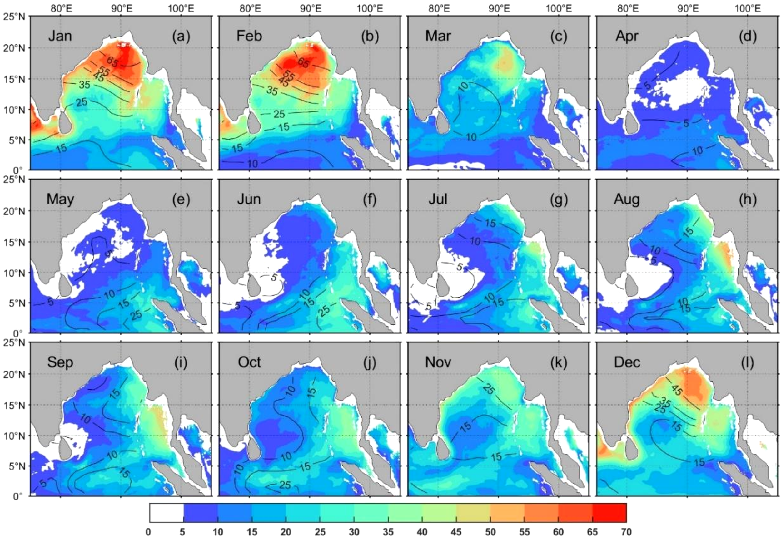
Monthly climatological BLT in the BoB from GLORYS12V1 product (shading) and Argo product (contours), in meters. The twelve subpanels (A–L) correspond to the months from January to December, respectively.
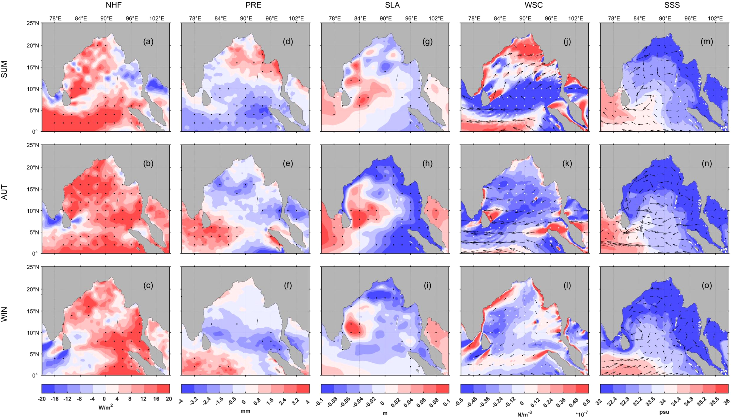
BLT is jointly determined by MLD and ILD. However, because the ILD is directly influenced only by temperature, the relative contributions of salinity are not considered for ILD. Therefore, to assess the roles of temperature and salinity in driving seasonal BLT variability, we first quantify their respective contributions to MLD. Here, the sign of each contribution indicates the effect direction of temperature or salinity changes on MLD relative to the climatological annual mean state. (i.e., a positive value of means that saline processes contribute to a deepening anomaly of the mixed layer, denoting a seasonally deeper MLD compared to the annual mean state). Notably, the salinity-related component includes all salinity-associated processes—such as precipitation, river discharge, and horizontal fresh/high-salinity water advection—rather than isolating individual terms. The results show that is significantly stronger than (Figures 2, 3), particularly in the equatorial and central BoB during summer (Figures 2F-I), where the saline process exerts a strong deepening effect. This may be linked to the intrusion of high-salinity waters from the Arabian Sea, as evidenced by the surface currents field shown in Supplementary Figures S4f–i, and also noted by Thadathil et al. (2007). Additionally, during the winter months (Figures 2A, B, L), salinity exerts substantial influence on the shallowing of the MLD in the northeastern BoB. By contrast, exhibits a pronounced positive anomaly (deeper than annual average MLD) in the equatorial region during summer (Figures 3f–i), but its influence remains significantly weaker than that of .
Figure 2
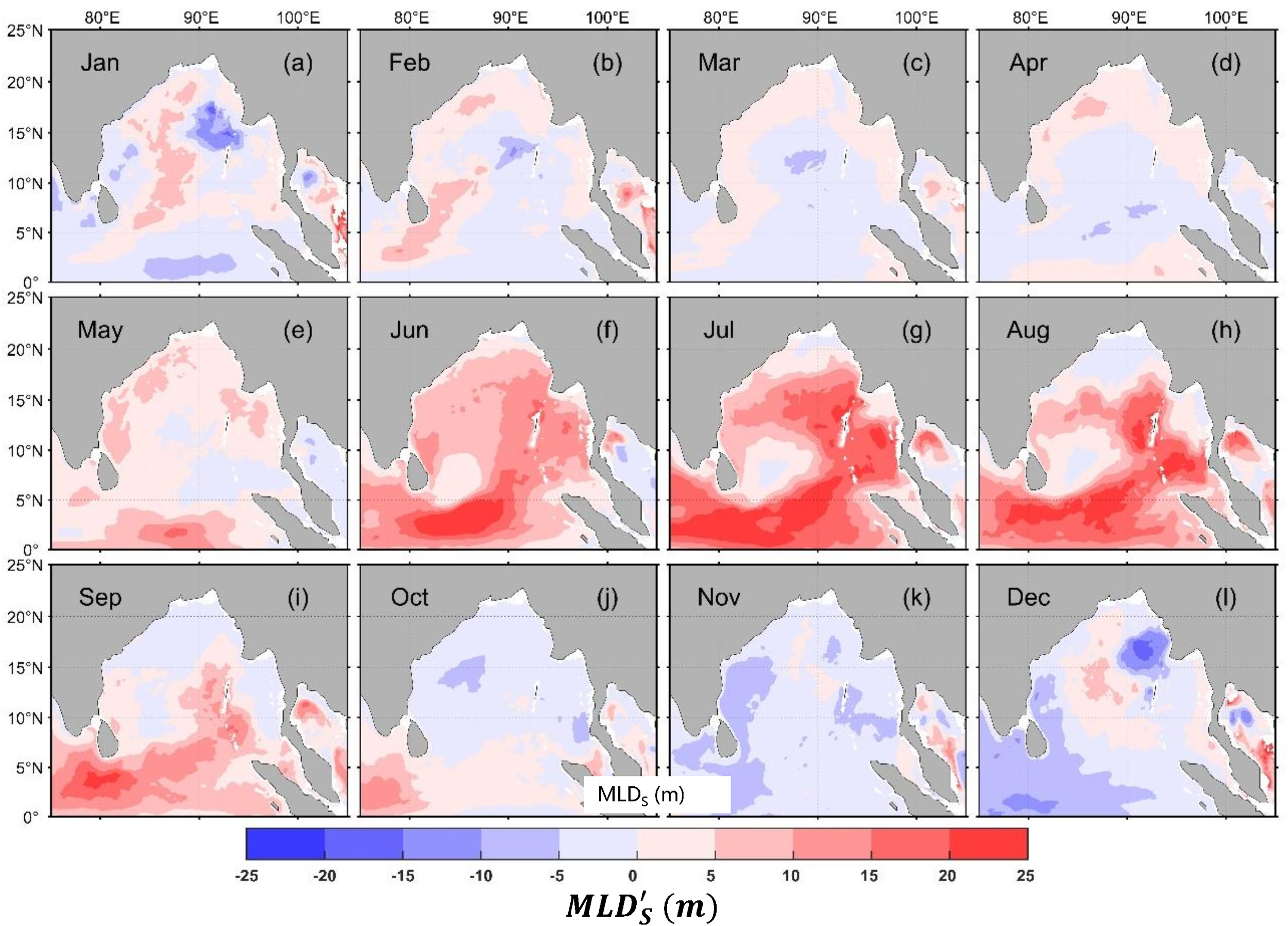
Monthly spatial distribution of relative to the climatological annual mean state in the BoB. The twelve subpanels (A–L) correspond to the months from January to December, respectively.
Figure 3
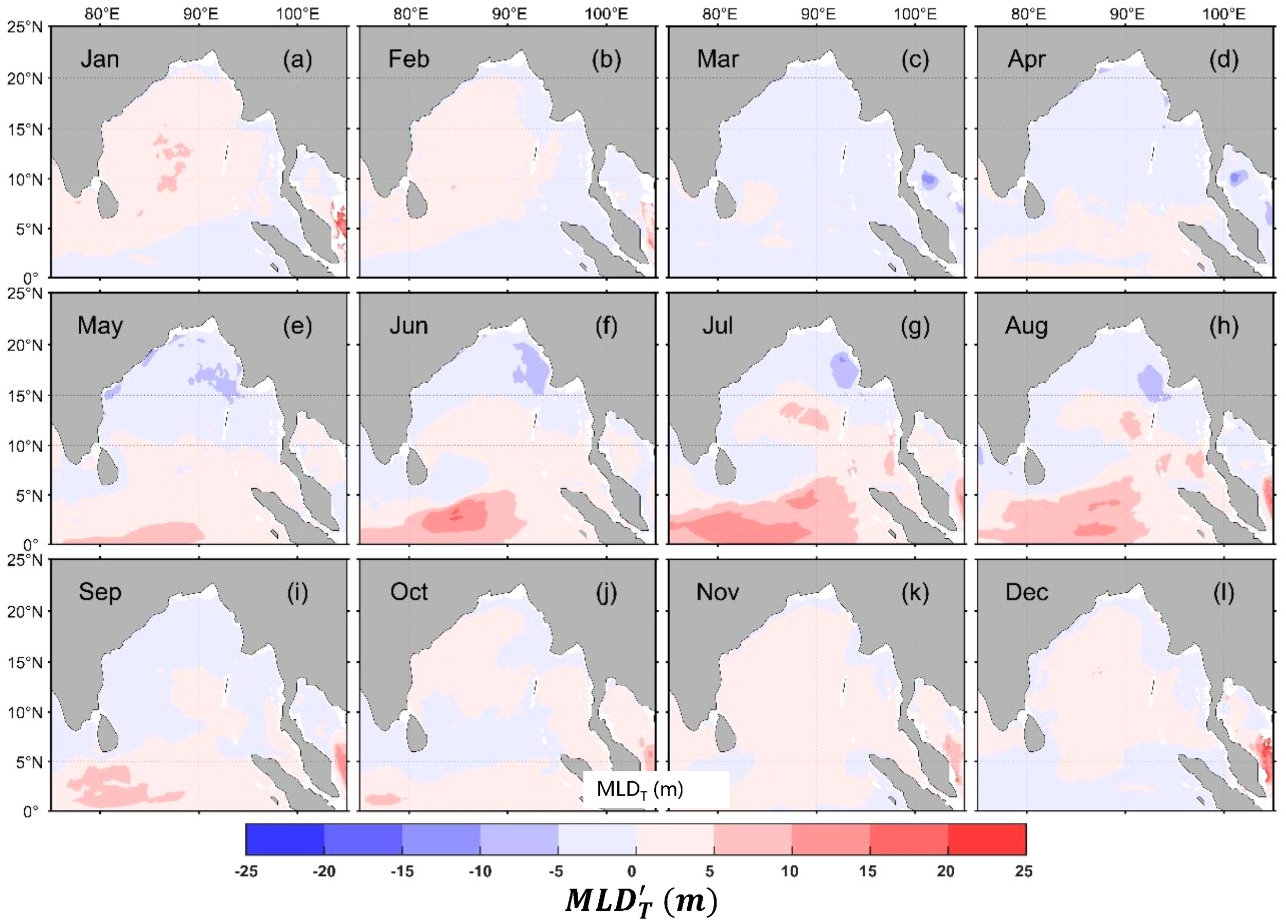
Monthly spatial distribution of relative to the climatological annual mean state in the BoB. The twelve subpanels (A–L) correspond to the months from January to December, respectively.
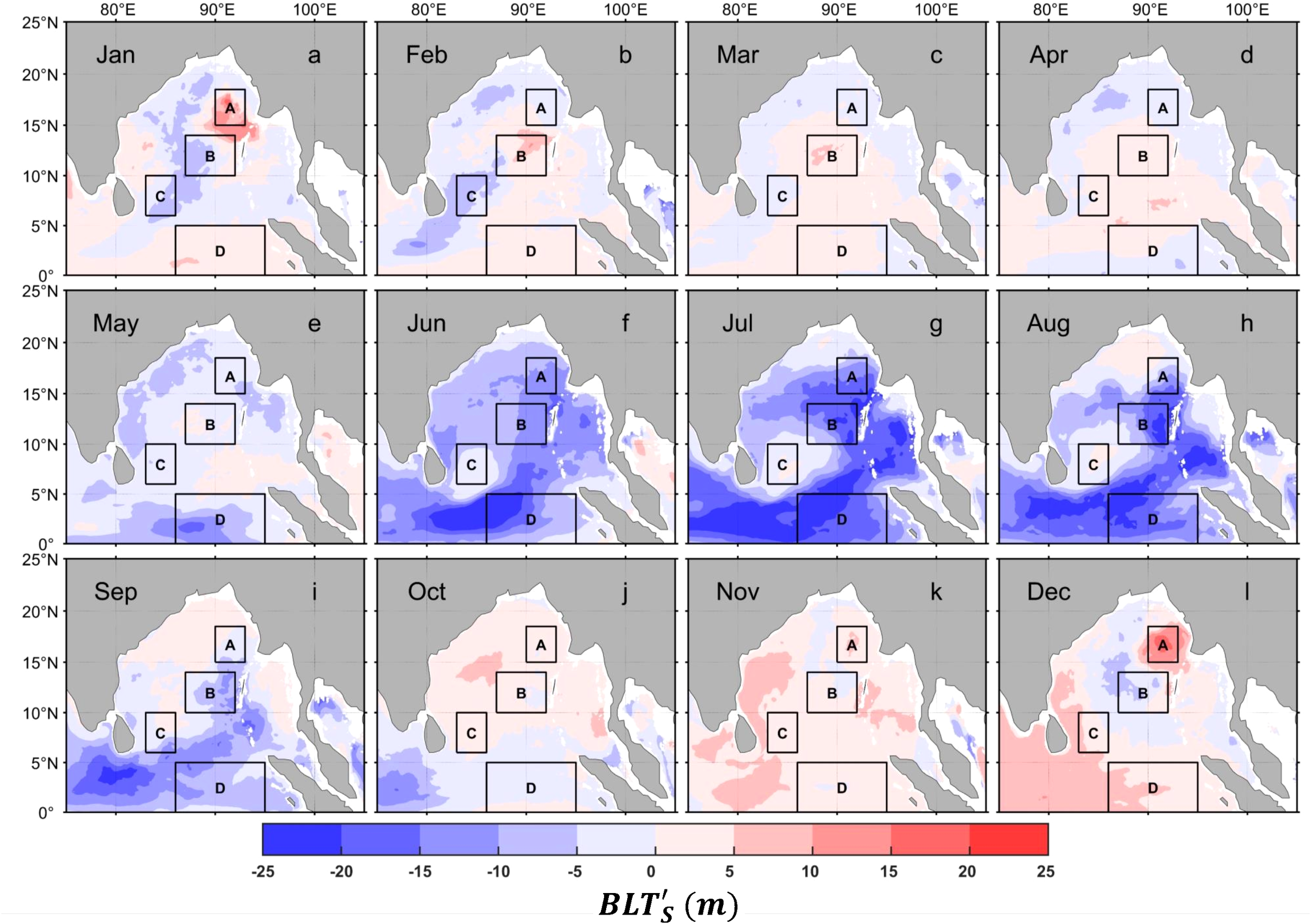
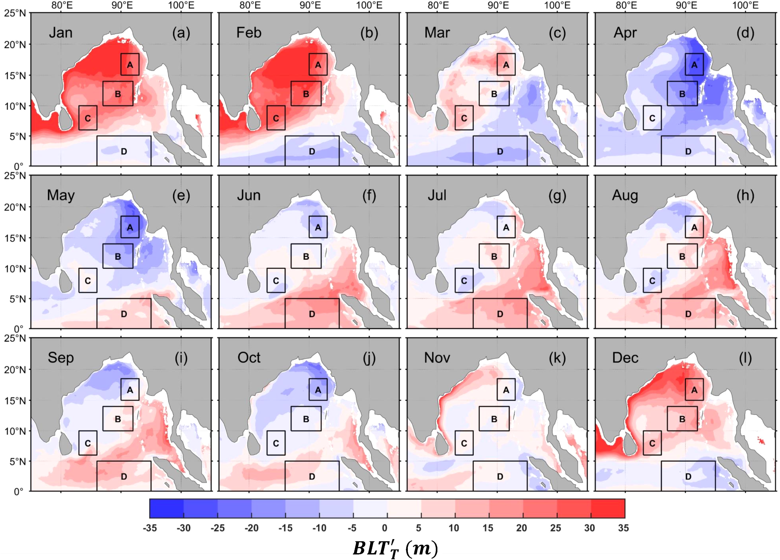
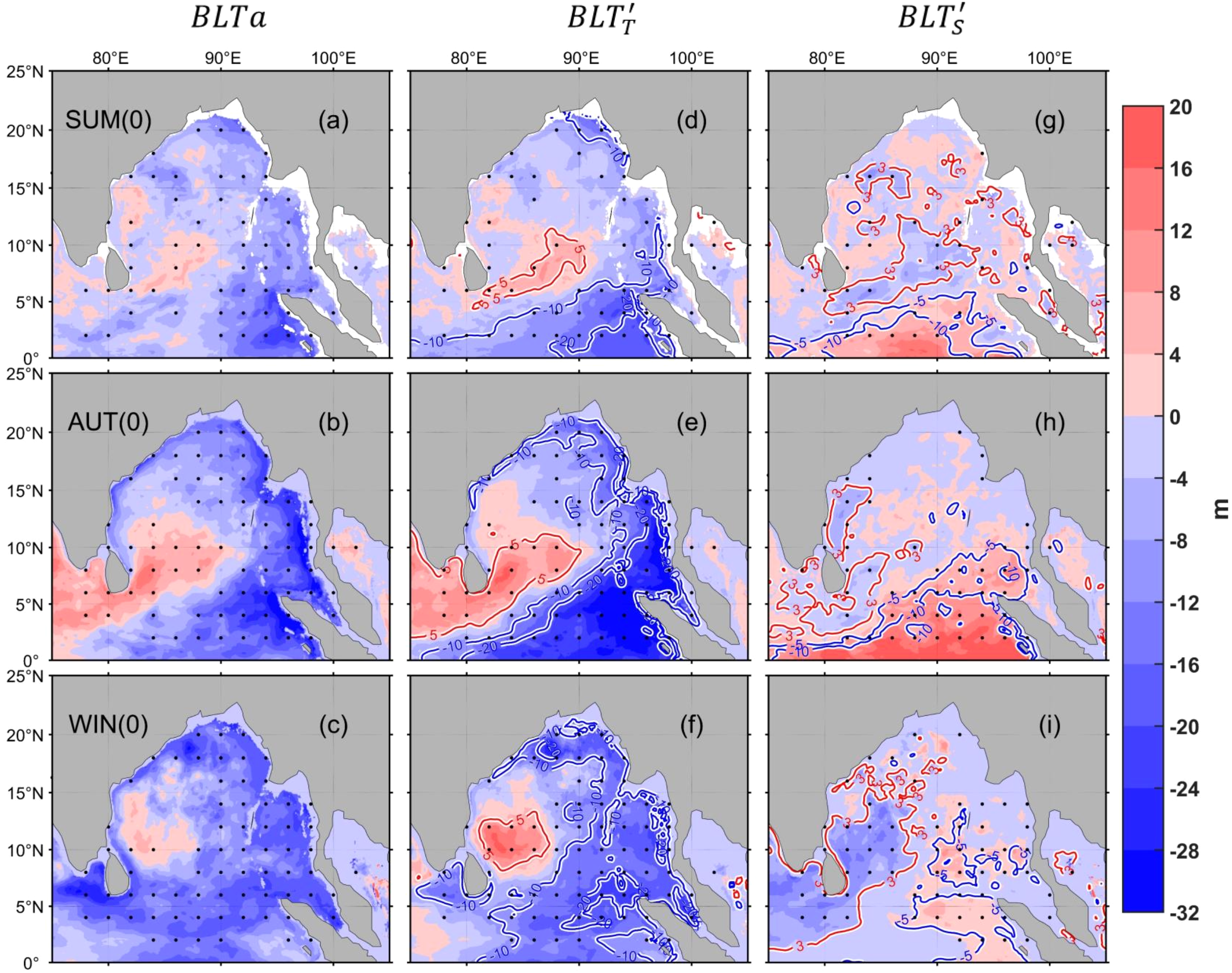
Building on the MLD analysis, we further examine the respective contributions of thermal and saline processes to the BLT by calculating and . To more intuitively illustrate the seasonal contrasts, we select four representative regions where the BLT changes are clear and the seasonal patterns are generally coherent (box A to D in Figures 4, 5, corresponding to typical areas in the northeast ern BoB, the central BoB, the area east of Sri Lanka, and the equatorial region, respectively). is similar to , with the strongest contribution during summer (Figures 5f–h) and the widest influence range, primarily leading to thinning through high-salinity waters intrusion. The strongest thinning occurs in the central bay and equatorial region, with average thinning of 11.1 m and 13.4 m in the region B and D, notably stronger than other seasons (Table 1). Additionally, saline processes also contribute to thinning in the western and central BoB during winter and along the coastal areas during spring, possibly due to reduced precipitation (Supplementary Figure S5), but this effect is significantly weaker compared to summer. In the northeastern part of the bay during winter, saline processes strongly contribute to thickening of the BLT, with an average thickening of approximately 6.6 m (Table 1), which is possibly due to the westward expansion of the Irrawaddy diluted water into the central BoB (Huang et al., 2025). Furthermore, for most areas during autumn and the central and southern BoB during spring, saline processes also thicken the BLT, but the intensity is weaker (Figure 4). is dominated by winter thickening inside the BoB, reaching 24.1 m in the northeastern bay—about twice the magnitude of the spring thinning (12 m) (Table 1). This thickening is likely associated with the monsoon-driven anticyclonic gyre and Ekman pumping that deepen the ILD (Supplementary Figure S4) (Thadathil et al., 2007). In contrast, thermal processes generally induce BLT thinning during other seasons, with the strongest reduction occurring in spring, likely due to enhanced net surface heat flux that strengthens thermal stratification and shoals the ILD (Supplementary Figure S3) and the buildup of warm water (Rao and Sivakumar, 1996). An exception occurs in the eastern equatorial region and the Andaman Sea, where thermal processes markedly thicken BLT in summer, which is possibly because the surface flow causes convergence and results in thick ILD (Supplementary Figure S4).
Figure 4
Monthly spatial distribution of relative to the climatological annual mean state in the BoB (Units in meters; Box A: 90-93°E, 15-18°N; Box B: 87-92°E, 10-14°N; Box C: 83-86°E, 6-10N; Box D: 86-95°E, 0-5°N). The twelve subpanels (A–L) correspond to the months from January to December, respectively.
Figure 5
Monthly spatial distribution of relative to the climatological annual mean state in the BoB (Units in meters; Box A: 90-93°E, 15-18°N; Box B: 87-92°E, 10-14°N; Box C: 83-86°E, 6-10N; Box D: 86-95°E, 0-5°N). The twelve subpanels (A–L) correspond to the months from January to December, respectively.
Table 1
| Study region | Spring (Mar. - May) | Summer (Jun.-Sep.) | Autumn (Oct.-Nov.) | Winter (Dec.-Feb.) |
|---|---|---|---|---|
| The northeastern BoB (Box A) | -1.6 m\-12.0 m | -8.4 m\-2.02 m | 2.5 m\-5.2 m | 6.6 m\24.1 m |
| The central BoB (Box B) | 2.0m\-9.6 m | -11.1 m\3.2 m | 1.2 m\0 m | -0.4 m\20.1 m |
| The region east of Sri Lanka (Box C) | -1.3 m\2.5 m | -1.6 m\-2.6 m | 2.4 m\0.3 m | -2.1 m\18.3 m |
| The eastern equatorial region (Box D) | -2.0 m\-2.4 m | -13.4 m\11.2 m | 0.8 m\1.6 m | 3.1 m\-4.2 m |
To visually compare and , we identify the spatial regions where either process primarily controls BLT variability. Specifically, at each grid point we take the absolute values of and , and divide the larger value by the smaller (| |/| | or | |/| |). A ratio greater than 2 indicates single-factor dominance, while a ratio less than 2 suggests joint control by both processes. As shown in Figure 6, during winter and spring, thermal processes dominate the thickening and thinning of the BLT inside the BoB, respectively, with a relatively large range (Figures 6A–E, L). In summer and autumn, they dominate the thinning in the northern BoB. Conversely, salinity dominates in the central BoB and the western equatorial region in summer, resulting in BLT thinning. Additionally, in the eastern equatorial region during summer, the combined influence of both processes leads to slight thickening of the BLT, arising from strong salinity-driven thinning counteracted by temperature-driven thickening (Figures 6F–I).
Figure 6
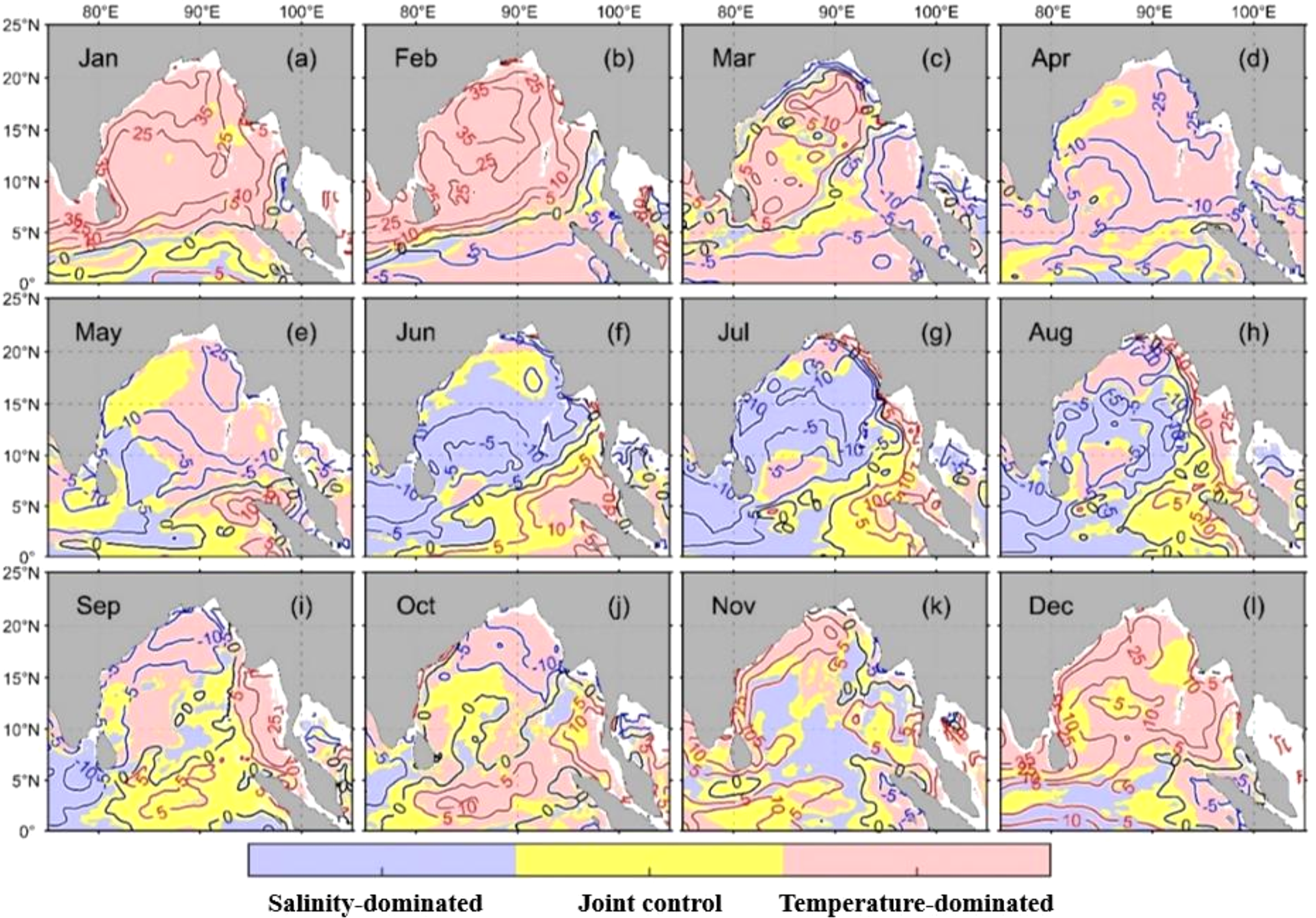
Dominant regions of thermal and saline processes affecting BLT variability (shading) and the monthly spatial distribution of BLT anomaly (contours, units in meters). The twelve subpanels (A–L) correspond to the months from January to December, respectively.
3.2 Interannual variability of BL in the BoB
Following the examination of seasonal variability, we turn to the interannual variability of BLT in the BoB to identify temporal patterns and regions of pronounced change. This variability is quantified as the annual standard deviation of BLT, highlighting regions where year-to-year changes are most pronounced. As shown in Figure 7A, the strongest interannual signals are found in the northern BoB and the eastern equatorial region, corresponding to the areas in the black box A and red box B. Temporally, interannual variability is more pronounced during autumn (September-November) and winter (December-February), and relatively weaker during spring (March-May) and summer (June-August) (Figure 7B).
Figure 7
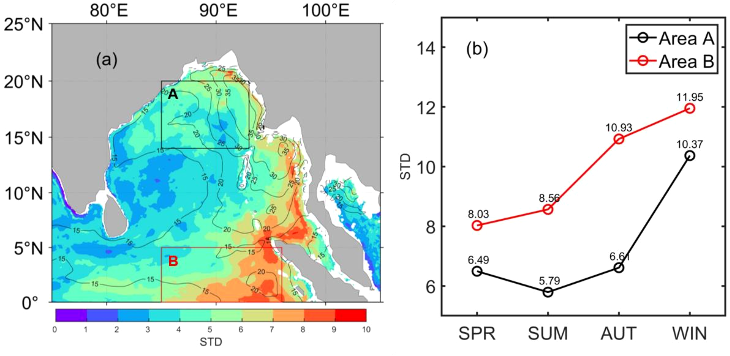
(A) Annual standard deviation (STD) of BLT in the BoB (shading) and climatological BLT (contours, units in meters). The black box A (83°E-92°E, 14°N-20°N) and the red box B (83°E-95°E, 0°-5°N) represent the northern BoB and equatorial regions, where significant interannual signals are strong. (B) STD of BLT for each season in the two regions.
Previous studies have found that the IOD and ENSO influence the interannual variability of the BLT in BoB, both exhibiting significant negative correlations with BLT variability across most regions of the BoB (Kumari et al., 2018; Valsala et al., 2018). However, these analyses were based on regional averages, making it difficult to resolve the spatial heterogeneity of IOD and ENSO effects. To address this limitation, we apply regression analysis at each grid point to investigate the spatial distribution of their impacts on BLT. Notably, in this section, interannual anomalies associated with IOD and ENSO events are defined as differences between composite event years and the corresponding climatological means.
3.2.1 IOD-driven interannual variability of BLT
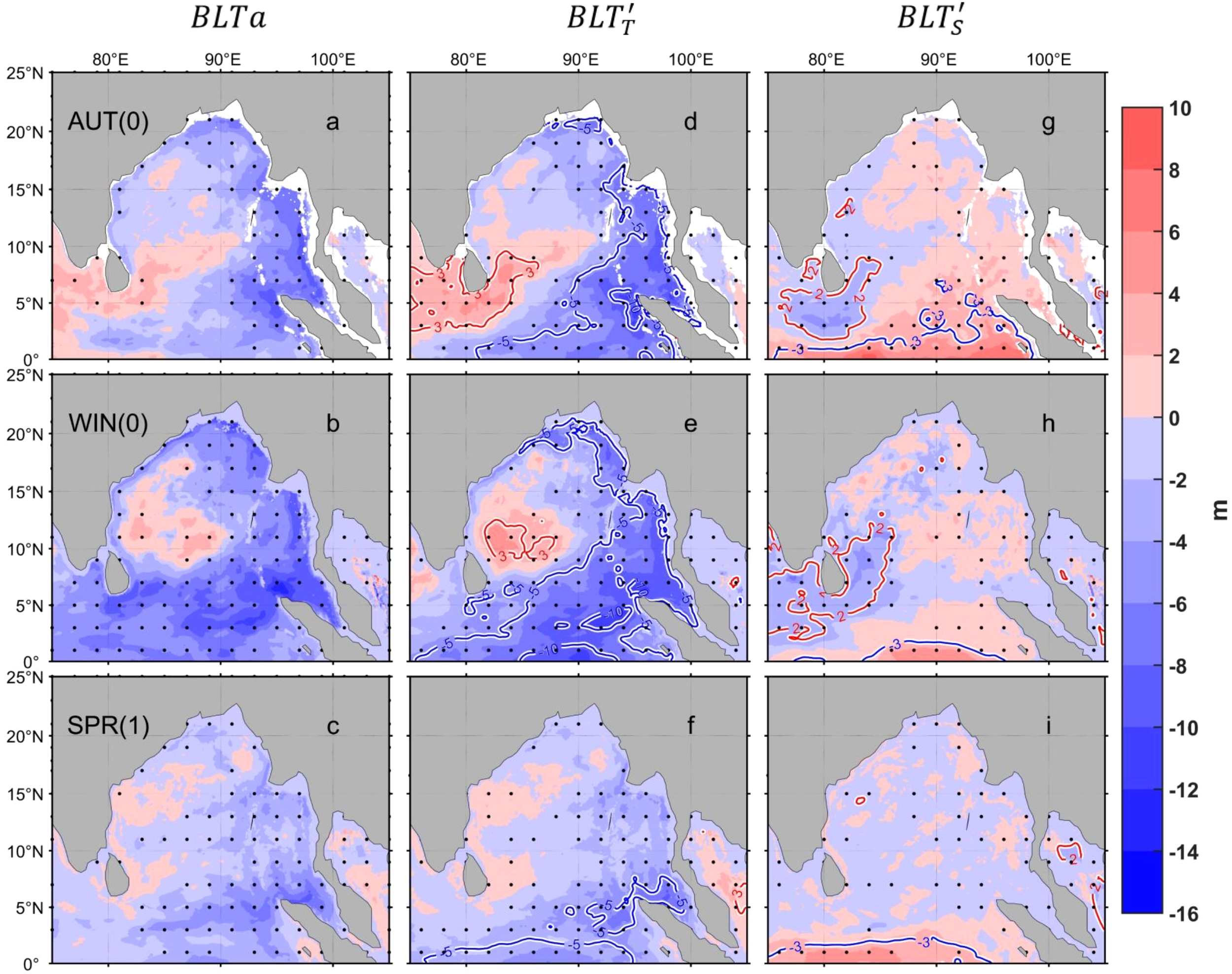
Since the IOD peaks in autumn, regression analyses are performed for the autumn IOD signal and BLT from summer to winter to distinguish between its effects during the development phase (summer) and the decay phase (winter). The impacts of IOD on interannual BLT variability in the BoB occurs mainly through the temperature-driven control of ILD. For instance, during pIOD events, in the equatorial region, the eastern BoB, and the northern BoB, the thermal process induces BLT thinning by raising ILD, with the strongest effect observed in the eastern equatorial region in autumn. Near Sri Lanka, the thermal process promotes BLT thickening by deepening of ILD, with the widest effect in autumn (Figures 8D–F). In contrast, the salinity-driven influence of IOD on BLT is generally weaker than that of the temperature. During the summer and autumn, the saline process contributes to BLT thickening by raising MLD in the equatorial region (Figures 8G–I), partly offsetting the temperature-induced thinning (Figures 8A–C). In winter, the saline process contributes to BLT thinning through deepening MLD near Sri Lanka (Figures 8G–I). In the northern region near Sri Lanka, this effects almost cancels out the temperature-driven thickening, whereas in the southern region, it reinforces the temperature-driven BLT thinning (Figures 8A–C). Collectively, the mechanisms by which the IOD affects BLT anomalies in the BoB are primarily governed by thermal processes, which regulate variations in ILD, while saline processes contribute locally through modulation of MLD.
Figure 8
Regressions of (A–C) interannual BLT anomaly, (D–F) (shading), (G–I) (shading) on autumn IODnoENSO in different seasons. Contours in (D–F) represent the regression of autumn IODnoENSO and ILD, and in (G–I) represent the regression with MLD. Dots indicate significance at the 95% confidence level.
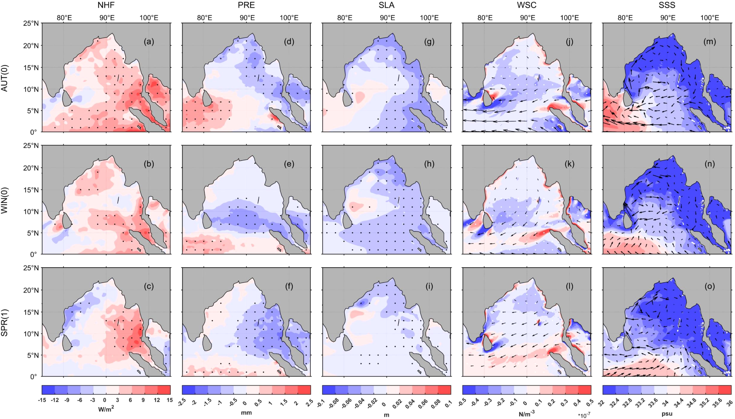
We further investigate the possible mechanisms by which the IOD affects the BLT in the BoB (Figure 9). During the pIOD period, for the thermal process, a positive net heat flux anomaly occurs in the eastern BoB, which increases the sea surface temperature and consequently raises the ILD. This contributes to BLT thinning. However, the spatial distribution of the net heat flux process is not entirely consistent the , indicating that net heat flux alone cannot entirely explain the impact of the IOD on BLT (Figures 8D–F, 9A–C).In contrast, the influence of the wind field exhibits a spatial pattern similar to , which may arise from two possible underlying mechanisms: On one hand, anomalous easterly winds excite upwelling Kelvin waves that travel north along the equator and the eastern BoB, while also radiating westward Rossby waves. These waves raise ILD along their paths, resulting in BLT thinning, with the strongest effect observed in the eastern equatorial region during autumn, consistent with . On the other hand, negative wind stress curl anomalies around Sri Lanka induce downward Ekman pumping, which deepens of the ILD and thus contributes to BLT thickening (Figures 9J–L). These are consistent with previous studies (Qiu et al., 2012; Ma et al., 2020). Regarding the saline process, in the pIOD period, stronger precipitation in the western equatorial region during autumn and winter (Figures 9D–F), dose not correspond with (Figures 8H, I) showing the saline process contribution to BLT thinning. This apparent inconsistency can be explained by changes in circulation. As the mechanism revealed by Sreenivas et al. (2012), anomalous easterlies suppress the downwelling Kelvin wave and consequently the southward-flowing East Indian Coastal Current (EICC) (Figure 9N), which is the primary mechanism for freshwater transport from the northern BoB. This reduction in freshwater supply, combined with intrusion of saltier water from the Arabian Sea in winter (Figures 9O), leads to a net surface salinity increase despite higher rainfall, ultimately resulting in ML deepening and BLT thinning. In the summer and autumn, westward currents transport low-salinity water from the Andaman Sea into the equatorial region of the BoB, which shallows MLD and thus contributes to BLT thickening (Figures 9M, N). Overall, the observed effects of the IOD on BLT are not driven directly by atmospheric forcing. Instead, they are primarily mediated by wind-induced Ekman dynamics and oceanic wave processes (Kelvin and Rossby waves), which modulate the internal ocean structure and drive the spatiotemporal evolution of BLT.
Figure 9
Regressions of autumn IODnoENSO with interannual in (A–C) net heat flux anomaly, (D–F) precipitation anomaly, (G–I) sea surface height anomaly, (J–L) wind stress curl anomaly (shading) and wind stress anomaly (vectors), (M–O) surface salinity (shading) and surface current anomaly (vectors). Dots indicate significance at the 95% confidence level.
3.2.2 ENSO-driven interannual variability of BLT
Similar to the IOD, regression analyses were performed for the winter ENSO signal and the BLT anomalies from autumn to the following spring to investigate its spatial and temporal impacts on BLT variability. ENSO primarily influences BLT variability through temperature-driven changes in ILD (Figure 10). During El Niño, the shoaling of the ILD induces BLT thinning in the equatorial ocean, the eastern BoB, and the northern BoB, while promoting BLT thickening around Sri Lanka (Figures 10D, E). By the following spring, this temperature effect weakens, resulting in only modest thinning in the equatorial and eastern BoB (Figure 10F). In contrast, saline processes exert a relatively weaker compensating or reinforcing effects through MLD changes. In the equatorial region, saline processes thicken BLT in autumn and winter, partly offsetting temperature-driven thinning. And around Sri Lanka, however, salinity effects act in the opposite direction, contributing to BLT thinning: nearly canceling the temperature-induced thickening in autumn, but enhancing thinning in winter. In spring, the salinity contribution becomes minor, producing only weak thickening near the equator, partially offsetting the thinning effect caused by thermal processes (Figures 10G–I).
Figure 10
Regressions of (A–C) interannual BLT anomaly, (D–F) (shading), (G–I) (shading) on winter ENSOnoIOD in different seasons. Contours in (D–F) represent the regression of winter ENSOnoIOD and ILD, and in (G–I) represent the regression with MLD. Dots indicate significance at the 95% confidence level.
We also investigated the possible mechanisms by which the ENSO affects the BLT in the BoB (Figure 11). Since the spatial patterns of net heat flux and precipitation do not correspond well with the observed BLT anomalies, they are not discussed further here. The influence of wind-driven processes on BLT under ENSO is similar to that of the IOD. For example, during El Niño events, wind-driven processes are well captured by : abnormal easterly winds lead to the northward propagating Kelvin waves along the equator and the eastern BoB, which raise the ILD and contribute to BLT thinning (Figures 11J–L). However, in the northern BoB during spring, BLT variability is weaker, as downward Ekman pumping induced by strong negative wind stress curl may offset the shoaling effect of Kelvin waves. Around Sri Lanka, in autumn and winter, the BLT is thickened due to the downward Ekman pumping (Figures 11J–L).
Figure 11
Regressions of winter ENSOnoIOD with interannual (A–C) net heat flux anomaly, (D–F) precipitation anomaly, (G–I) sea surface height anomaly, (J–L) wind stress curl anomaly (shading) and wind stress anomaly (vectors), and (M–O) surface salinity (vectors) and surface current anomaly (vectors). Dots indicate significance at the 95% confidence level.
Surface salinity advection could also effectively explain the influence of ENSO on BLT. During El Niño events, westward currents induced in equatorial BoB transport low-salinity water from the Andaman Sea, thereby thickening the BLT in autumn (Figures 11M). During La Niña periods, the opposite occurs: eastward currents carry high-salinity water from the Arabian Sea, leading to BLT thinning. Near Sri Lanka, in autumn and winter, El Niño-related northeastward currents bring high-salinity water from the Arabian Sea, promoting BLT thinning, whereas La Niña-related southwestward currents transport low-salinity water from the northern BoB, promoting BLT thickening (Figures 11M, N). Concurrently, in the west BoB, the mechanism as mentioned in Section 2.2.1 also appears: as demonstrated in Sreenivas et al. (2012), during El Niño years the anomalous easterlies suppress the second downwelling Kelvin wave. This suppression weakens EICC and thereby reduces the transport of low-salinity water from the northern BoB, leading to a higher surface salinity, a deeper mixed layer, and thus a thinner barrier. The anomalous current pattern also supports this interpretation (Figure 11M). Furthermore, this could also explain that the spatial extent of the negative contribution appears to be broader than that of (Figures 10b, c). This difference may arise because the Kelvin wave propagation directly influences the ILD and is a more coastal-trapped process, leading to a relatively localized response. In contrast, the weakened EICC affects salinity over a broader offshore region through its control on freshwater advection, resulting in a more extensive signature.
To synthesize the governing mechanisms of interannual BLT variability, we focus on the two periods when the influences of the IOD and ENSO are most pronounced — autumn for the IOD (Figure 8) and winter for ENSO (Figure 10). Figure 12 presents schematic diagrams summarizing the dominant processes during these key phases, represented by a pIOD event in autumn and an El Niño event in winter. In the panels, a stippled pattern indicates regions where temperature-driven processes dominate BLT variability, while a hatched pattern indicates salinity-dominated regions. During pIOD period, anomalous easterly winds excite upwelling Kelvin waves (blue arrow in Figure 12) and Rossby waves (blue curved arrow in Figure 12) that shoal the ILD, leading to BLT thinning in the eastern and northern bay. Concurrently, a negative wind stress curl anomaly induces downward Ekman pumping (red downward arrow), deepening the ILD and causing BLT thickening near Sri Lanka. In winter during El Niño event, anomalous easterlies also excite upwelling Kelvin waves and Rossby waves, causing large-scale BLT thinning in the eastern and northern bay. However, the wind stress curl anomaly associated with El Niño is more confined, and its impact on Ekman pumping is weaker and does not extend to the south and west regions of Sri Lanka. More importantly, in the southwest BoB, the BLT anomaly is dominated by saline processes: a weakened southward-flowing EICC (blue dashed arrow), which reduces the transport of freshwater from the north, and combined with the intrusion of high-salinity water from the Arabian Sea (blue arrow), leading to mixed layer deepening and BLT thinning.
Figure 12
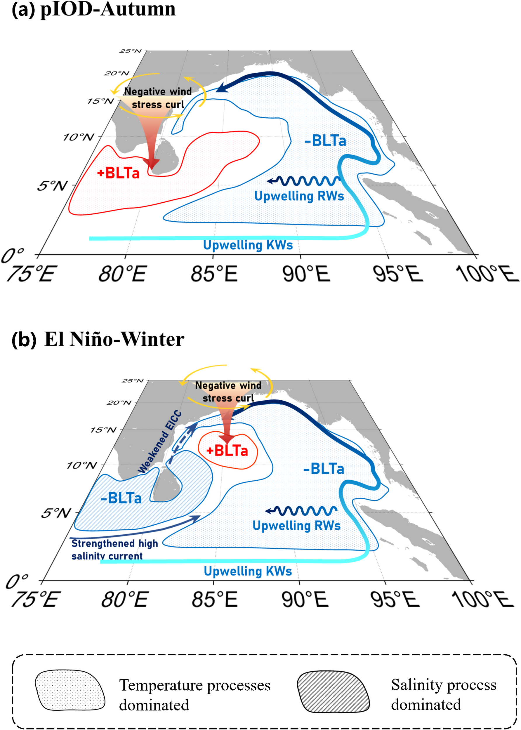
Schematic diagrams of the dominant processes affecting BLT variability in the Bay of Bengal during (A) the pIOD events in autumn and (B) El Niño events in winter.
4 Conclusions and discussions
This study used GLORYS12V1 and ERA5 products to quantify the relative contributions of temperature-driven and salinity-driven processes in regulating the seasonal and interannual variability of BLT in BoB. In both seasonal and interannual BLT variabilities, thermal processes, linked to monsoon circulation and equatorial waves, dominate the large-scale pattern and the associated variability, while salinity acts locally through freshwater transport and advection.
For seasonal variability, thermal processes dominate BLT variability in most region and seasons via monsoon-driven circulation and Ekman pumping that change the ILD. Saline processes are most influential in summer, contributing to BLT thinning in the central BoB and western equatorial region, largely due to the intrusion of high-salinity waters from the Arabian Sea. Interannual BLT variability is affected by IOD and ENSO through temperature-dominated ILD changes and salinity-modulated MLD changes. The IOD influences the BLT throughout its life cycle, from its development phase (summer) to decay phase (winter). During the pIOD events, thermal processes dominate the BLT thinning in the equatorial, eastern, and northern BoB, via the anomalous upwelling Kelvin waves and dominantly thicken BLT near Sri Lanka through downward Ekman pumping induced by the negative wind stress curl there. ENSO influences the BLT from autumn to the following spring also mainly by altering ILD. During El Niño events, the thermal processes predominantly cause BLT thinning in the equatorial, eastern, and northern BoB by thinning the ILD associated with the anomalous upwelling Kelvin waves, and cause BLT thickening near Sri Lanka via deepening ILD associated with the negative wind stress curl; saline process dominantly cause BLT thinning via deepening MLD due to the enhanced surface salinity by less fresh water transport associated with the weakening EICC.
By quantitatively isolating the contributions of thermal and saline processes, this study reveals more detailed features than previous qualitative studies and enables a clearer identification of the dominant controls on BLT across different regions and seasons in the BoB. Several of our findings are consistent with previous studies. For instance, the winter BLT thickening in the northern BoB, dominated by thermal processes, agrees well with the known mechanism of monsoon-driven circulation and Ekman pumping (Thadathil et al., 2007; Kumari et al., 2018). Similarly, the summer BLT thinning in the central and equatorial BoB, driven by salinity, supports the reported intrusion of high-salinity Arabian Sea water (Kumari et al., 2018). Beyond these consistencies, the explicit separation of temperature and salinity effects allows us to clarify several previously uncertain mechanisms. For instance, while several previous studies suggested that the BLT increase in the northeastern BoB during July–September might result from freshwater input (Masson et al., 2002; Kumari et al., 2018), our results indicate that this thickening is dominated by thermal process. Therefore, distinguishing between temperature and salinity contributions provides a more comprehensive understanding of the processes controlling BLT variability in the BoB.
By regressing BLT anomalies against IOD and ENSO indices at each grid point, this study reveals a more detailed spatial pattern of interannual variability. The results show that thermal processes dominate the BLT response through ILD variations, while salinity mainly acts locally to modulate MLD. Consistent to previous studies, during pIOD and El Niño events, the anomalous upwelling Kelvin waves cause BLT thinning in the equatorial and eastern BoB, whereas downwelling Ekman pumping around Sri Lanka leads to BLT thickening (Qiu et al., 2012; Ma et al., 2020). In addition to these agreements, the explicit separation of temperature and salinity effects enables a more precise diagnosis of the processes controlling BLT variability and helps clarify uncertain mechanisms. For example, during the pIOD phase, despite increased precipitation over the southwestern BoB, both SSSa and indicate higher surface salinity and BLT thinning. This apparent inconsistency can be explained by weakened southward freshwater transport due to the reduced strength of the EICC, which overwhelms the local freshening effect of rainfall, and leads to the thinning BLT. A similar mechanism operates during El Niño years. While our temperature-salinity decomposition effectively clarifies the dominant processes, a fully quantitative attribution of individual forcing components (e.g., heat flux, precipitation, and Ekman pumping) remains beyond the scope of the present approach. Future work incorporating targeted numerical sensitivity experiments would help to achieve a more detailed, mechanistic understanding.
In summary, this study quantifies the distinct contributions of thermal and saline processes to BLT variability in the BoB, clarifying their relative importance across seasons and under different climate modes. This quantitative separation proves critical for resolving previously uncertain mechanisms and deepening our understanding of how monsoon forcing and ocean circulation jointly regulate the upper-ocean structure. The findings provide a mechanistic basis for improving the simulation of BLT in ocean models, thereby supporting climate adaptation and disaster risk reduction efforts in South Asia and surrounding regions.
Statements
Data availability statement
The monthly GLORYS12V1 ocean reanalysis product dataset used in this study was obtained from https://data.marine.copernicus.eu/product/GLOBAL_MULTIYEAR_PHY_001_030/services. The ARGO data are available at http://apdrc.soest.hawaii.edu. ERA5 product is from https://www.ecmwf.int/en/forecasts/dataset/ecmwf-reanalysis-v5.
Author contributions
TL: Writing – original draft, Funding acquisition, Writing – review & editing, Validation. XN: Writing – review & editing, Data curation, Methodology, Visualization, Formal Analysis. YQ: Funding acquisition, Writing – review & editing, Conceptualization.
Funding
The author(s) declared financial support was received for this work and/or its publication. This work was funded by Scientific Research Foundation of, the National Natural Science Foundation of China (42130406), the Natural Science Foundation of Xiamen, China (3502Z202371037), the National Natural Science Foundation of China (U24A20607, 42506027), Scientific Research Foundation of Third Institute of Oceanography, MNR (2022027 and 2023014).
Acknowledgments
We would like to thank the reviewers for their time spent reviewing our manuscript and their comments that helped us improve this article.
Conflict of interest
The authors declared that this work was conducted in the absence of any commercial or financial relationships that could be construed as a potential conflict of interest.
Generative AI statement
The author(s) declared that generative AI was not used in the creation of this manuscript.
Any alternative text (alt text) provided alongside figures in this article has been generated by Frontiers with the support of artificial intelligence and reasonable efforts have been made to ensure accuracy, including review by the authors wherever possible. If you identify any issues, please contact us.
Publisher’s note
All claims expressed in this article are solely those of the authors and do not necessarily represent those of their affiliated organizations, or those of the publisher, the editors and the reviewers. Any product that may be evaluated in this article, or claim that may be made by its manufacturer, is not guaranteed or endorsed by the publisher.
Supplementary material
The Supplementary Material for this article can be found online at: https://www.frontiersin.org/articles/10.3389/fmars.2025.1721476/full#supplementary-material
References
1
Agarwal N. Sharma R. Parekh A. Basu S. Sarkar A. Agarwal V. K. (2012). Argo observations of barrier layer in the tropical Indian Ocean. Adv. Space Res.50, 642–654. doi: 10.1016/j.asr.2012.05.021
2
Balaguru K. Chang P. Saravanan R. Leung L. R. Xu Z. Li M. et al . (2012). Ocean barrier layers’ effect on tropical cyclone intensification. Proc. Natl. Acad. Sci.109, 14343–14347. doi: 10.1073/pnas.1201364109
3
Cai W. Rensch P. Cowan T. Hendon H. H. (2011). Teleconnection pathways of ENSO and the IOD and the mechanisms for impacts on Australian rainfall. J. Clim.24, 3910–3923. doi: 10.1175/2011JCLI4129.1
4
Cheng X. McCreary J. P. Qiu B. Qi Y. Du Y. (2017). Intraseasonal-to-semiannual variability of sea-surface height in the astern, equatorial Indian Ocean and southern Bay of Bengal. J. Geophys. Res. Oceans122, 4051–4067. doi: 10.1002/2016JC012662
5
Chowdary J. S. Parekh A. Ojha S. Gnanaseelan C. (2015). Role of upper ocean processes in the seasonal SST evolution over tropical Indian Ocean in climate forecasting system. Clim. Dyn.45, 2387–2405. doi: 10.1007/s00382-015-2478-4
6
de Boyer Montégut C. Mignot J. Lazar A. Cravatte S. (2007). Control of salinity on the mixed layer depth in the world ocean: 1. General description. J. Geophys. Res. Oceans112. doi: 10.1029/2006JC003953
7
Girishkumar M. S. Ravichandran M. McPhaden M. J. (2013). Temperature inversions and their influence on the mixed layer heat budget during the winters of 2006–2007 and 2007–2008 in the Bay of Bengal: THERMAL INVERSION IN THE BAY OF BENGAL. J. Geophys. Res. Oceans118, 2426–2437. doi: 10.1002/jgrc.20192
8
He Q. Zhan H. Cai S. (2020). Anticyclonic eddies enhance the winter barrier layer and surface cooling in the bay of bengal. J. Geophys. Res. Oceans125:e2020JC016524. doi: 10.1029/2020JC016524
9
Hersbach H. Bell B. Berrisford P. Horanyi A. Sabater J. (2019). Global reanalysis: goodbye ERA-Interim, hello ERA5. Available online at: https://www.ecmwf.int/en/elibrary/81046-global-reanalysis-goodbye-era-interim-hello-era5 (Accessed September 26, 2025).
10
Huang T. Zhou F. Xue L. Ye R. Meng Q. (2025). Impact of the irrawaddy diluted water on upper-layer salinity in the bay of bengal. J. Geophys. Res. Oceans130, e2025JC022939. doi: 10.1029/2025JC022939
11
Jean-Michel L. Eric G. Romain B.-B. Gilles G. Angélique M. Marie D. et al . (2021). The copernicus global 1/12° Oceanic and sea ice GLORYS12 reanalysis. Front. Earth Sci.9. doi: 10.3389/feart.2021.698876
12
Kumari A. Kumar S. P. Chakraborty A. (2018). Seasonal and interannual variability in the barrier layer of the bay of bengal. J. Geophys. Res. Oceans123, 1001–1015. doi: 10.1002/2017JC013213
13
Li J. Han D. Liao G. Zhang T. Ding R. Song X. (2024). Dynamics of the barrier layer dipole in the equatorial Indian ocean. J. Geophys. Res. Oceans129, e2023JC020479. doi: 10.1029/2023JC020479
14
Lindstrom E. Lukas R. Fine R. Firing E. Godfrey S. Meyers G. et al . (1987). The western equatorial pacific ocean circulation study. Nature330, 533–537. doi: 10.1038/330533a0
15
Liu Y. Li K. Ning C. Yang Y. Wang H. Liu J. et al . (2018). Observed seasonal variations of the upper ocean structure and air-sea interactions in the andaman sea. J. Geophys. Res. Oceans123, 922–938. doi: 10.1002/2017JC013367
16
Ma T. Cheng X. Qi Y. Chen J. (2020). Interannual variability in the barrier layer and forcing mechanism in the eastern equatorial Indian Ocean and Bay of Bengal. Acta Oceanol. Sin.39, 19–31. doi: 10.1007/s13131-020-1575-3
17
Masson S. Delecluse P. Boulanger J.-P. Menkes C. . (2002). A model study of the seasonal variability and formation mechanisms of the barrier layer in the eastern equatorial Indian Ocean. J. Geophys. Res. Oceans.107, SRF 18-1-20. doi: 10.1029/2001JC000832
18
Masson S. Luo J.-J. Madec G. Vialard J. Durand F. Gualdi S. et al . (2005). Impact of barrier layer on winter-spring variability of the southeastern Arabian Sea. Geophys. Res. Lett.32, L07703. doi: 10.1029/2004GL021980
19
Mignot J. Lazar A. Lacarra M. (2012). On the formation of barrier layers and associated vertical temperature inversions: A focus on the northwestern tropical Atlantic: BLS IN NORTHWESTERN TROPICAL ATLANTIC. J. Geophys. Res. Oceans117, C02010. doi: 10.1029/2011JC007435
20
Pathirana G. Wang D. Chen G. Abeyratne M. K. Priyadarshana T. (2022). Effect of seasonal barrier layer on mixed-layer heat budget in the Bay of Bengal. Acta Oceanol. Sin.41, 38–49. doi: 10.1007/s13131-021-1966-0
21
Qiu Y. Cai W. Guo X. Ng B. (2014). The asymmetric influence of the positive and negative IOD events on China’s rainfall. Sci. Rep.4, 4943. doi: 10.1038/srep04943
22
Qiu Y. Cai W. Li L. Guo X. (2012). Argo profiles variability of barrier layer in the tropical Indian Ocean and its relationship with the Indian Ocean Dipole. Geophys. Res. Lett.39, L08605. doi: 10.1029/2012GL051441
23
Qiu Y. Han W. Lin X. West B. J. Li Y. Xing W. et al . (2019). Upper-ocean response to the super tropical cyclone phailin, (2013) over the freshwater region of the bay of bengal. J. Phys. Oceanogr.49, 1201–1228. doi: 10.1175/JPO-D-18-0228.1
24
Qiu Y. Lin X. Jing C. (2021). Recurrence of wintertime SST anomalies in the Bay of Bengal: characteristics and causes. Clim. Dyn.57, 73–92. doi: 10.1007/s00382-021-05693-0
25
Rao R. R. Girish Kumar M. S. Ravichandran M. Rao A. R. Gopalakrishna V. V. Thadathil P. (2010). Interannual variability of Kelvin wave propagation in the wave guides of the equatorial Indian Ocean, the coastal Bay of Bengal and the southeastern Arabian Sea during 1993–2006. Deep Sea Res. Part Oceanogr. Res. Pap.57, 1–13. doi: 10.1016/j.dsr.2009.10.008
26
Rao R. R. Sivakumar R. (1996). Seasonal variability of near-surface isothermal layer and thermocline characteristics of the Tropical Indian Ocean. Meteorol. Atmospheric Phys.61, 201–212. doi: 10.1007/BF01025705
27
Rao R. Sivakumar R. (2003). Seasonal variability of sea surface salinity and salt budget of the mixed layer of the north Indian Ocean. J. Geophys. Res. C Oceans108, 9–1. doi: 10.1029/2001JC000907
28
Sheehan P. M. F. Matthews A. J. Webber B. G. M. Sanchez-Franks A. Klingaman N. P. Vinayachandran P. N. (2023). On the influence of the bay of bengal’s sea surface temperature gradients on rainfall of the south asian monsoon. J. Clim.36, 6499–6513. doi: 10.1175/JCLI-D-22-0288.1
29
Sreenivas P. Gnanaseelan C. Prasad K. V. S. R. (2012). Influence of El Niño and Indian Ocean Dipole on sea level variability in the Bay of Bengal. Glob. Planet. Change80–81, 215–225. doi: 10.1016/j.gloplacha.2011.11.001
30
Thadathil P. Muraleedharan P. M. Rao R. R. Somayajulu Y. K. Reddy G. V. Revichandran C. (2007). Observed seasonal variability of barrier layer in the Bay of Bengal. J. Geophys. Res. Oceans112, C02009. doi: 10.1029/2006JC003651
31
Thadathil P. Suresh I. Gautham S. Prasanna Kumar S. Lengaigne M. Rao R. R. et al . (2016). Surface layer temperature inversion in the Bay of Bengal: Main characteristics and related mechanisms: SURFACE LAYER TEMPERATURE INVERSION. J. Geophys. Res. Oceans121, 5682–5696. doi: 10.1002/2016JC011674
32
Valsala V. Prajeesh A. G. Singh S. (2022). Numerical investigation of tropical Indian ocean barrier layer variability. J. Geophys. Res. Oceans127, e2022JC018637. doi: 10.1029/2022JC018637
33
Valsala V. Singh S. Balasubramanian S. (2018). A modeling study of interannual variability of bay of bengal mixing and barrier layer formation. J. Geophys. Res. Oceans123, 3962–3981. doi: 10.1175/1520-0485(1998)028%3C1089:AOSFTT%3E2.0.CO;2
34
Vialard J. Delecluse P. (1998). An OGCM Study for the TOGA Decade. Part II: Barrier-Layer Formation and Variability. J. Phys. Oceanogr28, 1089–1106. doi: 10.1175/1520-0485(1998)028<1089:AOSFTT>2.0.CO;2
35
Vinayachandran P. N. Murty V. S. N. Ramesh Babu V. (2002). Observations of barrier layer formation in the Bay of Bengal during summer monsoon. J. Geophys. Res. Oceans107, SRF 19–1-SRF 19-9. doi: 10.1029/2001JC000831
36
Yuan X. Yu X. Su Z. (2020). Seasonal and interannual variabilities of the barrier layer thickness in the tropical Indian Ocean. Ocean Sci.16, 1285–1296. doi: 10.5194/os-16-1285-2020
37
Zheng F. Zhang R.-H. (2012). Effects of interannual salinity variability and freshwater flux forcing on the development of the 2007/08 La Niña event diagnosed from Argo and satellite data. Dyn. Atmospheres Oceans57, 45–57. doi: 10.1016/j.dynatmoce.2012.06.002
38
Zheng F. Zhang R.-H. Zhu J. (2014). Effects of interannual salinity variability on the barrier layer in the western-central equatorial Pacific: A diagnostic analysis from Argo. Adv. Atmospheric Sci.31, 532–542. doi: 10.1007/s00376-013-3061-8
Summary
Keywords
Bay of Bengal, barrier layer, seasonal variability, interannual variability, Indian Ocean Dipole, ENSO
Citation
Liu T, Ni X and Qiu Y (2026) Seasonal and interannual variability of the barrier layer in the Bay of Bengal: characteristics and mechanisms. Front. Mar. Sci. 12:1721476. doi: 10.3389/fmars.2025.1721476
Received
09 October 2025
Revised
25 November 2025
Accepted
10 December 2025
Published
16 January 2026
Volume
12 - 2025
Edited by
Samiran Mandal, Indian Institute of Technology Delhi, India
Reviewed by
Shang-Min Long, Hohai University, China
Sankar Prasad Lahiri, Indian Institute of Technology Delhi, India
Updates
Copyright
© 2026 Liu, Ni and Qiu.
This is an open-access article distributed under the terms of the Creative Commons Attribution License (CC BY). The use, distribution or reproduction in other forums is permitted, provided the original author(s) and the copyright owner(s) are credited and that the original publication in this journal is cited, in accordance with accepted academic practice. No use, distribution or reproduction is permitted which does not comply with these terms.
*Correspondence: Yun Qiu, qiuyun@tio.org.cn
Disclaimer
All claims expressed in this article are solely those of the authors and do not necessarily represent those of their affiliated organizations, or those of the publisher, the editors and the reviewers. Any product that may be evaluated in this article or claim that may be made by its manufacturer is not guaranteed or endorsed by the publisher.