Abstract
The classification of marine plankton images is of great significance in ecological studies and environmental monitoring. In practical applications, plankton image classification faces several challenges, including sample imbalance, distinguishing between-class and within-class differences, and recognizing fine-grained features. To address these issues, we propose a few-shot self-supervised transfer learning (FSTL) framework. In FSTL, we design a new loss function that incorporates both supervised and self-supervised learning. The core of FSTL is a hybrid learning objective that integrates self-supervised contrastive learning for robust feature representation. Operating within a transfer learning paradigm, FSTL effectively adapts knowledge from head-classes to boost the few-shot classification performance on tail-classes. We applied FSTL to two datasets, in which plankton images were collected from Daya Bay and provided by the Woods Hole Oceanographic Institution (WHOI) datasets respectively. The experimental results demonstrated that our method showed better adaptability in the classification of plankton images. The findings of this study not only apply to the classification of plankton images but also offer the potential for classifying small-sample categories within long-tailed datasets.
1 Introduction
Over the past three decades, in situ monitoring has generated vast amounts of data for marine plankton observation. Figure 1 shows images of four categories of marine plankton collected using this technique (Li et al., 2021). This surge in data has facilitated the application of machine learning and deep learning methods to the automated analysis of plankton image datasets (Benfield et al., 2007; MacLeod et al., 2010; Irisson et al., 2022). With advancements in convolutional neural networks (CNNs), deep learning methods have significantly enhanced feature extraction and image classification capabilities, thereby achieving classification tasks across various plankton image datasets (Lee et al., 2016; Li and Cui, 2016; Pedraza et al., 2017; Bochinski et al., 2019; Luo et al., 2018; Lumini and Nanni, 2019; Henrichs et al., 2021). However, their performance significantly degrades in real-world scenarios characterized by severe class imbalance and data scarcity. This is precisely the challenge of plankton image analysis.
Figure 1
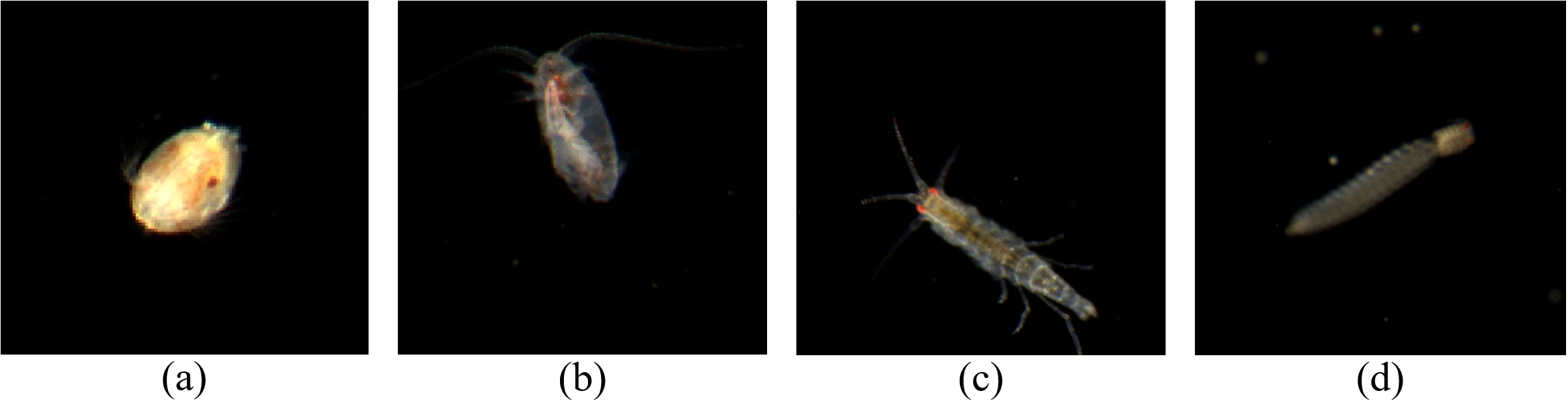
Marine plankton images of four categories from DYB dataset. (a) Ostracoda; (b) Calanoid Type B; (c) Gammarids Type A; (d) Polychaeta Type D.
The automated classification of plankton species faces intrinsic challenges because of morphological convergence, where phylogenetically distinct organisms exhibit similar global shapes. As depicted in the Figures 1a, b, the specimens share elliptical silhouettes but diverge in microstructural patterns. An analogous case occurs in the Figures 1c, d, both of which are elongated in shape. This necessitates models capable of capturing fine-grained morphological signatures beyond coarse shape attributes. Furthermore, intra-class morphological plasticity driven by imaging-angle variations amplifies the challenge. Identical species may present drastically different projections under oblique versus axial views, which demands the simultaneous modeling of inter-class separability and intra-class invariance.
Because of natural plankton distribution patterns and limitations in monitoring technology, some categories are frequently observed and well-represented (referred to as dominant or head class), whereas others contain only limited samples (known as disadvantaged or tail class). Figure 2 presents the sample sizes of different classes in the DYB dataset (Li et al., 2021), and clearly demonstrates a long-tailed distribution and data imbalance. Although CNNs possess powerful feature extraction capabilities, they are inherently biased toward head classes, leading to poor recognition of rare but ecologically important species. Standard transfer learning, which fine-tunes models pre-trained on large-scale datasets, often fails because the source and target domains are too distinct, and the model’s bias toward head classes persists. Similarly, class re-balancing strategies (e.g., re-sampling, loss re-weighting) are ineffective at the extreme “tail” of the distribution. These strategies require a minimum number of tail class samples to be effective, yet the core problem here is the sheer lack of such samples—many rare plankton categories have only a handful of instances, making re-balancing infeasible and often leading to overfitting. Motivated by these challenges, we introduce few-shot learning as a solution for this kind of data.
Figure 2
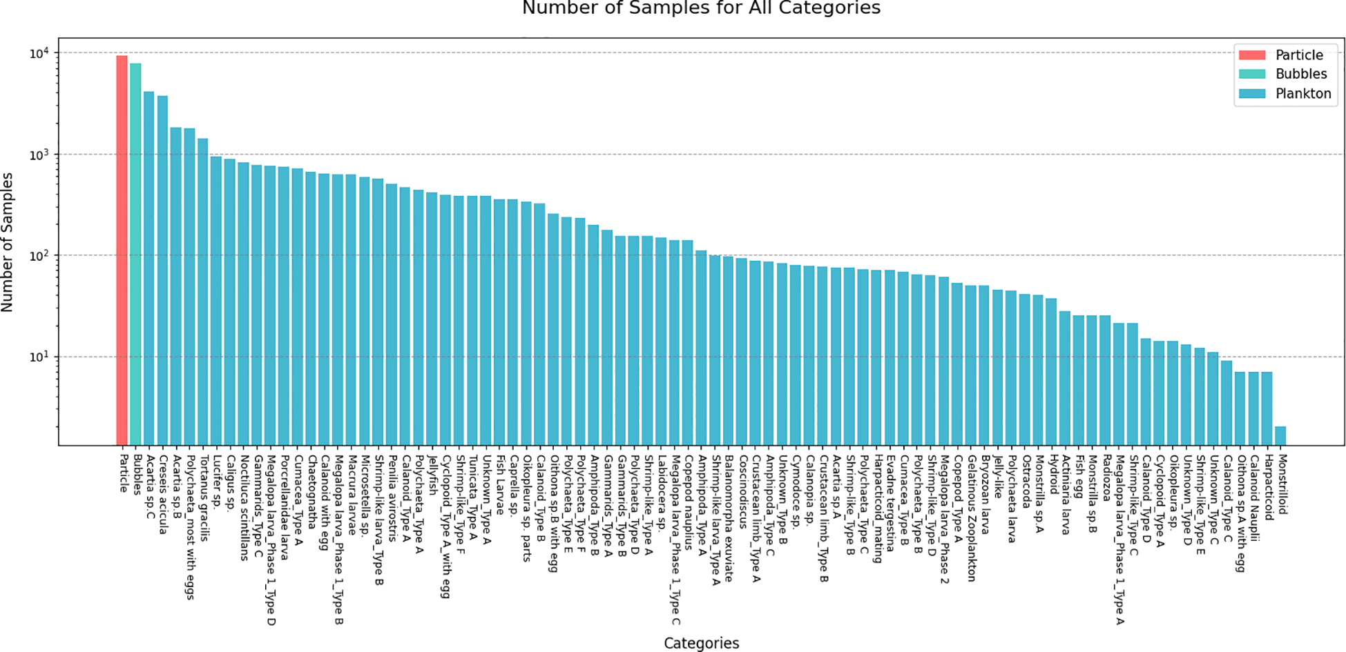
The long-tailed distribution of the DYB-plankton dataset.
Samples from tail classes are not only scarce but also often sparse, appearing infrequently and offering limited examples for model training. This sparsity obstructs effective feature extraction, which ultimately constrains the generalization capability. In this paper, the Few-shot Self-supervised Transfer Learning (FSTL) framework is designed to overcome these limitations by explicitly transferring robust feature representations from data-rich head classes to enable accurate classification of data-scarce tail classes. First, we train the model on head-class data, and subsequently fine-tune it on tail-class data, with the goal of developing a classification model that performs effectively on tail-class data. To address these issues, we propose a novel loss function for FSTL and investigate the selection of hyperparameters. The main contribution of this paper can be summarized as follows: (1) We design a novel FSTL framework to achieve few-shot classification on marine plankton images. (2) Through a carefully designed toy experiment, we further demonstrate the robustness of FSTL in handling low-quality plankton images. The results confirm that our proposed loss function enhances classification accuracy, particularly for the tail class with limited samples, highlighting the method’s capability to address practical challenges in marine image analysis.
The rest of this paper is organized into four sections. Section 2 describes related work. Section 3 details the proposed FSTL framework and its new loss function. Section 4 evaluates the method by comparing it with baselines on two main datasets and a toy example. Section 5 concludes with a discussion.
2 Related works
2.1 Few-shot classification
Wang et al. (2020) identified the core challenge of few-shot learning as the disparity between the small sample size and the complexity of the data. Two common approaches for addressing this challenge are data augmentation and model architecture redesign.
For data augmentation, Miller et al. (2000) leveraged similarities between existing categories to learn geometric transformations, thus enriching the small sample size dataset. Kwitt et al. (2016) developed a set of independent attribute strength regressors based on scene images with fine-grained annotations. Additionally, generative adversarial networks (GANs) (Gao et al., 2018) and autoencoders (Schwartz et al., 2018) are also commonly used in data augmentation.
Few-shot learning models, such as model-agnostic meta-learning (MAML) (Finn et al., 2017), first-order meta-learning (Reptile) (Nichol and Schulman, 2018), and Prototypical Network (Snell et al., 2017), have been widely applied and achieved promising results. Sun et al. (2019) combined meta-learning and transfer learning to achieve meta-transfer learning, and proposed a more advanced version for few-shot fine-grained classification (Sun et al., 2020). Another promising method for small-sample image classification is self-supervised learning, which can learn useful feature representations from data without relying on labels. Related methods can be divided into self-supervised generative learning and self-supervised contrastive learning (SCL) (Albelwi, 2022; Chen et al., 2020; Lim et al., 2023; Su et al., 2020; He et al., 2020). However, the methods mentioned above were not tailored for marine plankton images, overlooking their distinctive characteristics, particularly the fine-grained nature of the classification task.
2.2 Long-tailed learning
Recently, several effective long-tailed learning strategies have emerged: (Kang et al., 2020) decoupled representation and classifier learning; (Shi et al., 2023) revealed the limitations of re-sampling under contextual bias and introduced context-shift augmentation; (Aditya et al., 2021) boosted tail-class performance via logit adjustment; and (Cui et al., 2019) designed a class-balanced loss based on effective sample numbers. The aforementioned methods all operate under the premise that the training set itself has a long-tailed distribution. In contrast, in this paper, we aim to address the few-shot problem in the tail classes not by directly training on the tail data, but by training on the head classes and leveraging a transfer learning idea. While recent transfer-learning works (You et al., 2020; Atanov et al., 2022) also explore head-to-tail knowledge transfer by re-using the source classifier, they are not designed to handle fine-grained details or low-clarity images. Our method therefore differs in both objective and technical focus, extending transfer learning to the challenging scenario of plankton classification with very few samples.
2.3 Plankton image classification
In addition to sample imbalance, classification methods also need to address issues such as distinguishing between-class and within-class differences, as well as recognizing fine-grained features. Additionally, because of the difficulty in obtaining plankton images, the available datasets are limited, and related research is still in its early stages. Lee et al. (2016) proposed a fine-grained plankton classification method based on CNNs. Wang et al. (2017) introduced a model based on GANs, which mitigates class imbalance in plankton image datasets by generating samples for few-shot categories. Schröder et al. (2018) applied weight imprinting techniques to enable neural networks to recognize the tail class without the need for retraining. Sun et al. (2020) proposed a feature fusion model that uses a focal region localization mechanism to identify perceptually similar areas between objects and extract discriminative features. Guo et al. (2023) addressed distribution differences between few-shot and non-few-shot classes, adopting a cross-domain few-shot classification approach.
Although existing methods have achieved certain results in few-shot plankton image classification, they have not incorporated self-supervised learning. This is particularly important for fine-grained tasks like plankton classification, which is a key motivation and contribution of our adoption of self-supervise contrastive learning in this work.
3 Methodology
3.1 Problem formulation
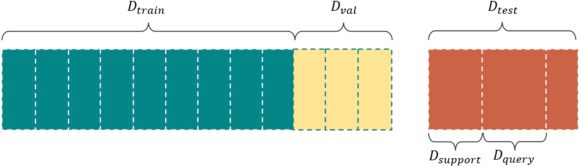
The proposed method is in a framework of few-shot classification using transfer learning. As shown in Figure 3, a few-shot classification task involves two datasets: the training set and test set , where and represent the sample and its corresponding label, respectively. When dealing with long-tailed datasets, Dtrain corresponds to the head-class with sufficient samples, whereas Dtest corresponds to the tail-class with sparse samples. N and Nt epresent the sample sizes of these two datasets, respectively, and N ≫ Nt. C categories are chosen from Dtest and S samples are selected from each category to form . Then, the remaining samples of the C chosen categories become . Therefore, Dsupport and Dquery share the same label space, which is disjoint from the label space of Dtrain. Such a few-shot classification task can be referred to as a C-way S-shot task.
Figure 3
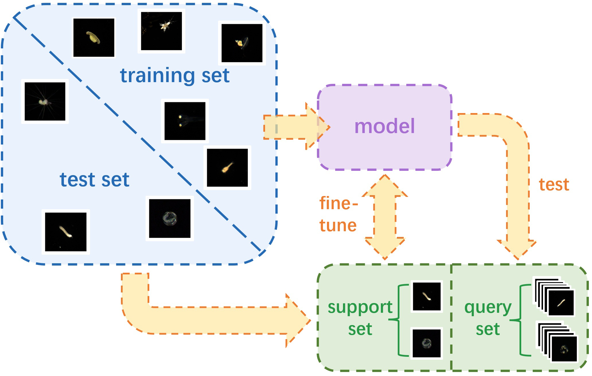
Framework of few-shot learning.
Few-shot classification aims to learn a transferable model M1 on Dtrain, which can be further fine-tuned using Dsupport to obtain model M2. Finally, we test the few-shot classification accuracy of model M2 on the query set Dquery.
3.2 Self-supervised learning framework of FSTL
FSTL improves the original loss function of SCL (Lim et al., 2023) and obtains a lightweight loss function that performs better in extracting features of plankton images at a fine-grained level and reflecting differences between classes.
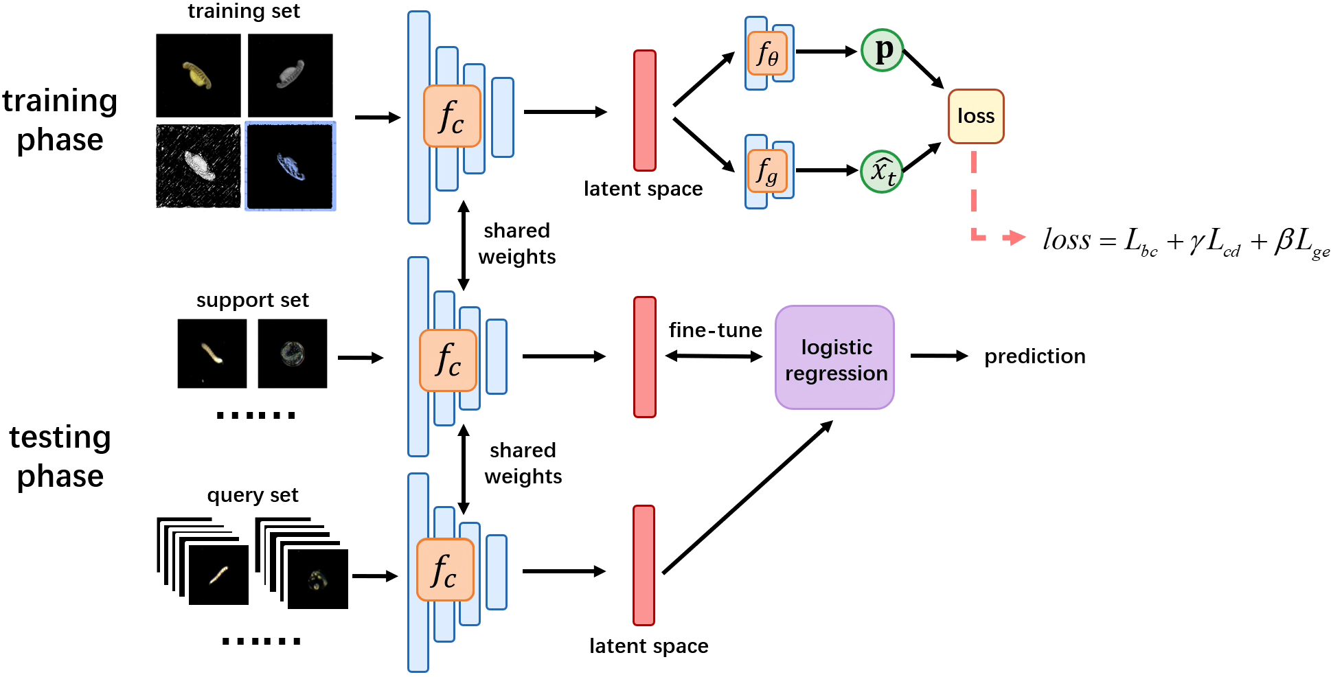
As shown in Figure 4, the core of FSTL is a self-supervised feature extractor fc, which is built on ResNet-12. fc can map a two-dimensional image to a latent space and use a one-dimensional vector to represent the extracted image features. In the training phase, both supervised and self-supervised learning are used to create a classification task and a generation task, respectively. Then, the classifier fθ and generator fg are used to compute a loss function, whose minimization yields the optimal estimates of parameters in fc, fθ, and fg. In the testing phase, all parameters in fc are no longer changed, and fc converts samples from Dsupport and Dquery into feature vectors. Then a logistic regressor is trained on Dsupport. Its classification accuracy on Dquery is tested.
Figure 4
The overall design of FSTL.
3.2.1 Classification task
For an image sample x in Dtrain, data augmentation transformations and rotation transformations are applied to generate three derived images from x. The original image x and its three derived images (rotate 90°, 180°, 270°) are concatenated into a tensor x. Similarly, a class label vector y is obtained, whose four components share the same value. This process results in a new dataset .
We use a single-layer fully connected network to implement the classifier fθ. The feature extractor fc transforms a single image into a feature vector v first, then fθ outputs a class prediction vector . The length of is equal to the number of categories in the total dataset and the sum of all its elements is equal to 1. By maximizing the overall performance of fθ, we force fc to focus on between-class differences, thus improving the quality of the extracted features.
3.2.2 Generation task
The generator fg is composed of a lightweight CNN. Each sample x in Dtrain undergoes a data augmentation transformation T, which produces an augmented version xt. The augmented image is then fed into fc to form a feature vector . Using vector v and fg, a generated image is produced. The goal of the generation task is to find the optimal fc and fg such that the difference between xt and is minimized. The generation task forces fc to pay more attention to pixel-level differences within the images, further improving the ability of fine-grained classification. Figure 4 shows the overall design of FSTL.
3.2.3 Loss function
During the training phase, the tensor sample from is fed into to obtain the corresponding feature tensor , where each element represents the corresponding from four rotations (). Next, the feature tensor is input into the classifier to obtain the class label prediction tensor . Simultaneously, is also input into the generator to obtain .
A loss function consisting of three parts (named CCM loss) is proposed. By minimizing this loss function, the optimal parameters of fc, fθ, and fg can be obtained.
where Lbc in Equation 1 is the cross-entropy loss function with respect to the class label yi and class label prediction vector , which enhances the feature extractor fc’s ability to discriminate between classes. It is defined in Equation 2,
where represents the th element in vector . is a cosine similarity loss function for , see Equation 3,
where cos< ·,· > denotes the cosine similarity function. Lcd aims to bring the feature vectors of different samples with the same label as close as possible, thereby enabling the feature extractor fc to learn invariant features within a category. Lge represents the mean squared error (MSE) between the augmented image xt and the generated image :
where in Equation 4, MSE is a binary function that takes tensors as input and computes the mean of the squared differences between corresponding elements of the input tensors. Lge allows the loss function L in (1) to focus more on pixel-level feature differences, thereby enhancing fc’s ability to recognize subtle feature variations.
In the CCM loss function (1), γ and β are two hyperparameters used to control the model’s tendencies during the learning process. The model M1 is trained according to Equation 5.
where c, θ, and g denote the trainable parameters in fc, fθ, and fg, respectively.
3.2.4 Difference between FSTL and SCL
The structure of SCL is similar to that of FSTL, with the main difference being that SCL does not have a generation task. There are two classification tasks in the training phase of SCL: one for category labels and the other for rotation labels; in FSTL, we do not use the rotation label.
The loss function of SCL also consists of three terms in Equation 6.
where Equation 7 is
In the loss function of SCL (6), the first term is the same as that of FSTL, and the last two terms are determined by the result of the two classification tasks. However, the third term in the loss of SCL is totally different from that of FSTL, where riis the rotation parameter (). Additionally, FSTL replaces the binary norm with cosine similarity in the second term in the loss function.
In summary, the effectiveness of our framework stems from the following aspects. First, by incorporating the self-supervised contrastive learning, we empower the model with a more powerful feature representation capability, which is crucial for fine-grained classification. Second, we enhance this foundation by designing a novel loss function with two dedicated terms: Lbc sharpens the model’s focus on between-class differences, while Lge directs attention to pixel-level, within-class variations. These components work synergistically within a transfer learning paradigm, enabling knowledge acquired from the head class to be effectively adapted for analyzing the tail class, thereby achieving robust few-shot classification of plankton images.
4 Experiment
4.1 Datasets
We use two datasets to conduct experiments. The DYB-plankton dataset, collected from Daya Bay in Shenzhen (Li et al., 2021), contains 93 classes, including various plankton species and non-biological particles such as bubbles and debris. After classes with fewer than 20 samples are removed, 74 classes remain. The WHOI-plankton dataset, provided by the Woods Hole Oceanographic Institution (https://hdl.handle.net/10.1575/1912/7341), contains 53 classes after the exclusion of classes with fewer than 20 samples. Images in both datasets are normalized to a size of 84×84 pixels.
To achieve the partition of datasets, a residual neural network is initially used to classify all categories in the datasets. The 10 classes with relatively lower accuracy are selected as Dtest (these 10 classes are with small sample sizes), and the remaining constitute Dtrain. Samples for the support set Dsupport and query set Dquery are selected from Dtest based on the C-way S-shot experimental setting introduced in Section 3.1. To prevent overfitting during the training phase, a validation set Dval is separated from Dtrain in a 1:3 ratio, as shown in Figure 5.
Figure 5
Partition of datasets.
For the DYB dataset, classes containing over 500 samples are subsampled to 500 images each via random selection. All available images from smaller classes are included. Subsequently, the data are partitioned into training and testing subsets in a 4:1 ratio, and then a ResNet model was used for classification.
Although the overall test set accuracy reached 85.96%, 20 classes exhibited test accuracy below 50%. We randomly selected 10 of these classes as Dtest for the subsequent few-shot experiments. Their sample sizes and classification accuracy is listed in Table 1. We applied a similar approach to the WHOI dataset. The results are listed in Table 2.
Table 1
| Index of category | Sample size | Accuracy | Index of category | Sample size | Accuracy |
|---|---|---|---|---|---|
| 1 | 80 | 28.57% | 6 | 45 | 0% |
| 2 | 76 | 18.18% | 7 | 44 | 25% |
| 3 | 72 | 28.57% | 8 | 37 | 39.13% |
| 4 | 70 | 35.71% | 9 | 28 | 25% |
| 5 | 50 | 40% | 10 | 25 | 50% |
Accuracy of each category in the test set of the DYB dataset.
Table 2
| Index of category | Sample size | Accuracy | Index of category | Sample size | Accuracy |
|---|---|---|---|---|---|
| 1 | 107 | 20.00% | 6 | 44 | 0% |
| 2 | 66 | 23.53% | 7 | 35 | 25.00% |
| 3 | 61 | 0% | 8 | 24 | 18.18% |
| 4 | 58 | 10.53% | 9 | 22 | 0% |
| 5 | 55 | 0% | 10 | 22 | 9.09% |
Accuracy of each category in the test set of the WHOI dataset.
4.2 Experimental settings
4.2.1 Data augmentation
The following data augmentation (T) methods are used: 1) random cropping of the image with a scale ratio between 0.5 and 1.0, and then resizing it back to the original size using bilinear interpolation; 2) application of random color jitter with an 80% probability, involving random adjustments to brightness, contrast, saturation, and hue; and 3) conversion of the image to grayscale with a 20% probability.
4.2.2 Feature extractor
The feature extractor fc is built using ResNet-12. This network consists of four residual blocks, each containing three convolutional layers. Each convolutional layer has 64 convolutional filters with a (3, 3) kernel. A max-pooling layer with a size of (2, 2) is added after the last convolutional layer in the first three residual blocks. Following the fourth residual block, a global average pooling layer is applied. To prevent overfitting, the DropBlock (Ghiasi et al., 2018) technique is used, with block sizes of (64, 160, 320, 640).
4.2.3 Classifier
In the training phase, fθ is a simple classifier that consists of a fully connected layer. The input consists of the feature vectors, and the output size varies depending on the number of classes in the few-shot classification task.
4.2.4 Generator
In the training phase, the generator fg is a lightweight convolutional network. It includes a fully connected layer to upsample the feature vectors, followed by four convolutional layers that transform the upsampled feature vectors back to the original image size. The convolutional layers have the following sizes in sequence: (64, 32, 3, 3), (32, 16, 3, 3), (16, 3, 3, 3), and (3, 3, 5, 5).
4.2.5 Logistic regressor
In the testing phase, the logistic classifier is a single-layer neural network. The feature vectors are fed into the network and a softmax function is applied to obtain a probability score for each class. The class with the highest score is selected as the predicted label.
4.2.6 Optimization strategy
During the training phase, the feature extractor fc, classifier fθ, and generator fg can be considered as three sub-blocks of one neural network, which allows them to share the same optimizer. The network is optimized using the SGD optimizer. The initial learning rate is set to 0.05, with an L2 penalty coefficient of 5e−4, and the batch size is set to 32. The maximum number of iterations is set to 100, and the learning rate is multiplied by 0.1 at the 60th and 80th iterations.
During the testing phase, all parameters of fc remain fixed. Initially, fc converts the images in Dsupport into their corresponding feature vectors. A logistic regression classifier is then trained on these extracted features to perform multi-class classification.
The classifier is optimized using the L-BFGS algorithm, using an L2 penalty term with a maximum iteration number limit of 1000. Finally, the entire assembled model is evaluated on Dquery to assess its generalization performance.
All experiments were conducted on a high-performance workstation equipped with six NVIDIA GeForce RTX 3090 GPUs (each with 24GB memory), totaling 144GB GPU memory. The training process utilized multiple GPUs in parallel. The average GPU utilization was above 60%, and the power consumption was approximately 300W per card under full load. All experiments were conducted under Python 3.8, PyTorch 2.1.2 and CUDA 12.2.
4.3 Metrics
In classification tasks, accuracy and precision are two commonly used metrics. They are generally applied to binary classification tasks, where samples are typically labeled as either positive or negative. Their calculation is shown in Equations 8, 9, and TP, FP, TN, and FN correspond to the true positive rate, false positive rate, true negative rate, and false negative rate, respectively.
When the number of categories exceeds three, it is necessary to use macro-accuracy and macro-precision. For a specific category k, we label all samples that belong to that category as positive and label all samples that do not belong to it as negative. This approach enables us to calculate accuracy and precision for each category individually, which allows us to obtain the overall macro-accuracy and macro-precision. S denotes the number of categories in Dquery, and the calculation is as Equation 10, 11:
4.4 Experimental results
To thoroughly evaluate the performance of FSTL, we designed three experiments. In Experiment 1, we tested four existing few-shot classification methods on plankton images. The results demonstrated that SCL (Lim et al., 2023) achieved the best performance among them. Experiment 2 involved comparing the performance of FSTL and SCL for various hyperparameter settings, which demonstrated the effectiveness of FSTL in the context of plankton few-shot classification. Finally, Experiment 3 was a preliminary investigation of the relationship between the performance of FSTL and the quality of the images used.
4.4.1 Experiment 1
We used four state-of-the-art few-shot classification models as baseline methods: SCL (Lim et al., 2023), MAML (Finn et al., 2017), prototypical network (Snell et al., 2017), and relation network (Sung et al., 2018).
We evaluated the classification performance of these four baselines on the DYB and WHOI datasets. The results for the DYB dataset are presented in Tables 3, 4. The experimental results indicate that SCL achieved the highest performance among the baselines. Therefore, we primarily compare the performance of SCL with that of FSTL.
Table 3
| Configuration | SCL | MAML | Prototypical network | Relation network |
|---|---|---|---|---|
| 5-way 1-shot | 72.69 | 52.70 | 42.61 | 51.80 |
| 5-way 3-shot | 84.66 | 63.43 | 54.71 | 63.79 |
| 5-way 5-shot | 87.81 | 67.70 | 60.08 | 66.58 |
| 5-way 10-shot | 91.17 | 73.83 | 63.98 | 69.06 |
| 10-way 1-shot | 59.48 | 35.38 | 27.82 | 35.66 |
| 10-way 3-shot | 73.99 | 42.85 | 35.65 | 46.70 |
| 10-way 5-shot | 78.86 | 48.80 | 39.59 | 50.60 |
| 10-way 10-shot | 84.01 | 57.60 | 41.44 | 53.48 |
Macro-accuracy of different methods on DYB query set.
Table 4
| Configuration | SCL | MAML | Prototypical network | Relation network |
|---|---|---|---|---|
| 5-way 1-shot | 74.95 | 53.47 | 45.85 | 53.11 |
| 5-way 3-shot | 86.04 | 64.80 | 57.38 | 65.32 |
| 5-way 5-shot | 88.86 | 68.85 | 61.98 | 68.28 |
| 5-way 10-shot | 91.99 | 75.15 | 65.03 | 75.01 |
| 10-way 1-shot | 61.97 | 35.47 | 30.79 | 37.15 |
| 10-way 3-shot | 76.49 | 44.70 | 38.41 | 48.91 |
| 10-way 5-shot | 80.51 | 50.20 | 41.48 | 53.31 |
| 10-way 10-shot | 85.35 | 59.23 | 43.01 | 58.10 |
Macro-precision of different methods on DYB query set.
4.4.2 Experiment 2
We compared the performance of FSTL and SCL for various hyperparameter settings. For each C-way S-shot experiment, we randomly sampled Dsupport from Dtest. We repeated this process 2,000 times to calculate the average macro-accuracy and average macro-precision. The results are presented in Tables 5–8. The values in parentheses represent the half-length of the 95% confidence interval for each metric.
Table 5
| Model configuration | 5-way 1-shot | 5-way 3-shot | 5-way 5-shot | 5-way 10-shot | 10-way 1-shot | 10-way 3-shot | 10-way 5-shot | 10-way 10-shot | Average |
|---|---|---|---|---|---|---|---|---|---|
| FSTL | |||||||||
| Lbc | 72.69 (0.43) | 84.66 (0.31) | 87.81 (0.26) | 91.17 (0.22) | 59.48 (0.25) | 73.99 (0.17) | 78.86 (0.15) | 84.01 (0.16) | 79.08 |
| Lbc + Lcd | 71.83 (0.43) | 84.68 (0.30) | 87.86 (0.26) | 90.07 (0.24) | 59.73 (0.24) | 73.93 (0.18) | 78.73 (0.15) | 84.19 (0.16) | 78.88 |
| Lbc + Lge | 72.69 (0.43) | 84.76 (0.30) | 87.64 (0.26) | 91.34 (0.22) | 58.92 (0.26) | 73.75 (0.17) | 78.84 (0.15) | 84.17 (0.15) | 79.01 |
| Lbc + 1.5Lge | 71.98 (0.42) | 84.65 (0.30) | 88.06 (0.25) | 91.39 (0.22) | 59.52 (0.25) | 73.16 (0.18) | 78.61 (0.15) | 82.62 (0.16) | 78.75 |
| Lbc + Lcd + Lge | 72.73 (0.42) | 84.51 (0.31) | 87.10 (0.26) | 91.38 (0.22) | 59.12 (0.25) | 73.56 (0.17) | 78.55 (0.15) | 84.44 (0.15) | 78.92 |
| Lbc + Lcd + 1.5Lge | 72.18 (0.43) | 83.87 (0.33) | 87.48 (0.25) | 90.81 (0.22) | 60.41 (0.24) | 73.55 (0.17) | 79.23 (0.15) | 84.20 (0.15) | 78.97 |
| SCL | |||||||||
| Lbc | 72.69 (0.43) | 84.66 (0.31) | 87.81 (0.26) | 91.17 (0.22) | 59.48 (0.25) | 73.99 (0.17) | 78.86 (0.15) | 84.01 (0.16) | 79.08 |
| Lbc + Lbr | 72.39 (0.43) | 84.20 (0.31) | 87.65 (0.27) | 90.00 (0.24) | 57.98 (0.24) | 72.57 (0.18) | 77.36 (0.15) | 83.88 (0.15) | 78.25 |
| 57.79 (0.53) | 68.27 (0.42) | 72.01 (0.37) | 75.56 (0.34) | 44.41 (0.28) | 53.82 (0.19) | 57.61 (0.17) | 64.78 (0.19) | 61.78 | |
Query set macro-accuracy on DYB dataset.
Table 6
| Model configuration | 5-way 1-shot | 5-way 3-shot | 5-way 5-shot | 5-way 10-shot | 10-way 1-shot | 10-way 3-shot | 10-way 5-shot | 10-way 10-shot | Average |
|---|---|---|---|---|---|---|---|---|---|
| FSTL | |||||||||
| Lbc | 74.95 (0.45) | 86.04 (0.29) | 88.86 (0.24) | 91.99 (0.21) | 61.97 (0.30) | 76.49 (0.18) | 80.51 (0.15) | 85.35 (0.15) | 80.77 |
| Lbc + Lcd | 74.08 (0.44) | 86.16 (0.28) | 88.93 (0.24) | 90.96 (0.23) | 62.23 (0.29) | 75.91 (0.19) | 79.71 (0.15) | 85.51 (0.16) | 80.44 |
| Lbc + Lge | 75.00 (0.44) | 85.84 (0.30) | 88.64 (0.24) | 92.10 (0.21) | 61.70 (0.29) | 75.92 (0.18) | 80.76 (0.15) | 85.60 (0.14) | 80.70 |
| Lbc + 1.5Lge | 74.35 (0.46) | 85.90 (0.29) | 89.00 (0.23) | 92.15 (0.20) | 62.27 (0.29) | 75.12 (0.19) | 80.40 (0.15) | 84.02 (0.16) | 80.40 |
| Lbc + Lcd + Lge | 74.93 (0.45) | 85.91 (0.29) | 88.19 (0.24) | 92.17 (0.20) | 61.39 (0.30) | 75.97 (0.18) | 80.29 (0.15) | 85.71 (0.14) | 80.57 |
| Lbc + Lcd + 1.5Lge | 74.67 (0.45) | 85.31 (0.30) | 88.54 (0.23) | 91.68 (0.20) | 63.00 (0.29) | 75.77 (0.18) | 80.76 (0.15) | 85.63 (0.15) | 80.67 |
| SCL | |||||||||
| Lbc | 74.95 (0.45) | 86.04 (0.29) | 88.86 (0.24) | 91.99 (0.21) | 61.97 (0.30) | 76.49 (0.18) | 80.51 (0.15) | 85.35 (0.15) | 80.77 |
| Lbc + Lbr | 74.88 (0.44) | 85.67 (0.29) | 88.75 (0.25) | 90.92 (0.22) | 60.70 (0.29) | 74.76 (0.19) | 78.40 (0.15) | 85.15 (0.15) | 79.90 |
| 59.07 (0.57) | 69.82 (0.44) | 73.59 (0.38) | 77.19 (0.35) | 44.81 (0.32) | 54.37 (0.24) | 58.67 (0.20) | 66.79 (0.22) | 63.04 | |
Query set macro-precision on DYB dataset.
Table 7
| Model configuration | 5-way 1-shot | 5-way 3-shot | 5-way 5-shot | 5-way 10-shot | 10-way 1-shot | 10-way 3-shot | 10-way 5-shot | 10-way 10-shot | Average |
|---|---|---|---|---|---|---|---|---|---|
| FSTL | |||||||||
| Lbc | 60.89 (0.43) | 75.37 (0.31) | 79.45 (0.27) | 83.89 (0.25) | 48.30 (0.28) | 62.08 (0.21) | 68.75 (0.17) | 74.48 (0.18) | 69.15 |
| Lbc + Lcd | 61.37 (0.43) | 75.35 (0.31) | 79.42 (0.28) | 84.15 (0.25) | 49.01 (0.28) | 63.63 (0.21) | 69.92 (0.17) | 74.52 (0.17) | 69.67 |
| Lbc + Lge | 60.08 (0.43) | 74.40 (0.33) | 79.22 (0.28) | 83.74 (0.25) | 47.15 (0.28) | 62.56 (0.21) | 68.61 (0.17) | 74.39 (0.18) | 68.77 |
| Lbc + 1.5Lge | 60.51 (0.43) | 74.92 (0.32) | 79.50 (0.26) | 83.58 (0.26) | 48.05 (0.27) | 63.79 (0.21) | 68.69 (0.17) | 75.05 (0.18) | 69.26 |
| Lbc + Lcd + 1.5Lge | 60.81 (0.42) | 74.60 (0.32) | 79.99 (0.27) | 83.69 (0.25) | 48.81 (0.28) | 63.78 (0.20) | 68.66 (0.17) | 74.91 (0.17) | 69.41 |
| Lbc + Lcd + 2Lge | 61.14 (0.43) | 75.36 (0.31) | 79.41 (0.27) | 83.79 (0.26) | 48.66 (0.28) | 63.65 (0.20) | 68.70 (0.17) | 74.10 (0.17) | 69.35 |
| SCL | |||||||||
| Lbc | 60.89 (0.43) | 75.37 (0.31) | 79.45 (0.26) | 83.89 (0.22) | 48.30 (0.25) | 62.08 (0.17) | 68.75 (0.15) | 74.48 (0.16) | 69.15 |
| Lbc + Lbr | 60.14 (0.43) | 74.20 (0.31) | 78.61 (0.27) | 83.47 (0.24) | 47.28 (0.24) | 61.61 (0.18) | 67.92 (0.15) | 73.58 (0.15) | 68.35 |
| 57.41 (0.53) | 72.04 (0.42) | 77.30 (0.37) | 82.56 (0.34) | 43.32 (0.28) | 57.25 (0.19) | 63.02 (0.17) | 70.20 (0.19) | 65.39 | |
Query set macro-accuracy on WHOI dataset.
The bold values indicate that these experimental results are superior to the results obtained by using only the first term of the loss function.
Table 8
| Model configuration | 5-way 1-shot | 5-way 3-shot | 5-way 5-shot | 5-way 10-shot | 10-way 1-shot | 10-way 3-shot | 10-way 5-shot | 10-way 10-shot | Average |
|---|---|---|---|---|---|---|---|---|---|
| FSTL | |||||||||
| Lbc | 62.97 (0.46) | 77.54 (0.30) | 81.34 (0.27) | 85.57 (0.24) | 50.64 (0.34) | 64.94 (0.24) | 71.19 (0.18) | 77.05 (0.19) | 71.41 |
| Lbc + Lcd | 63.83 (0.49) | 77.47 (0.31) | 81.21 (0.27) | 85.84 (0.23) | 51.49 (0.34) | 66.19 (0.23) | 72.65 (0.18) | 77.11 (0.17) | 71.97 |
| Lbc + Lge | 62.83 (0.48) | 76.43 (0.32) | 81.08 (0.27) | 85.35 (0.24) | 49.43 (0.34) | 65.63 (0.23) | 71.42 (0.18) | 76.81 (0.18) | 71.12 |
| Lbc + 1.5Lge | 63.18 (0.48) | 77.13 (0.32) | 81.38 (0.25) | 85.29 (0.24) | 50.65 (0.33) | 66.34 (0.23) | 71.45 (0.18) | 77.61 (0.17) | 71.63 |
| Lbc + Lcd + 1.5Lge | 62.97 (0.48) | 76.71 (0.32) | 81.77 (0.26) | 85.45 (0.23) | 51.29 (0.33) | 66.60 (0.23) | 71.08 (0.18) | 77.49 (0.17) | 71.67 |
| Lbc + Lcd + 2Lge | 63.68 (0.49) | 77.38 (0.32) | 81.11 (0.26) | 85.45 (0.25) | 50.94 (0.33) | 66.33 (0.23) | 71.28 (0.19) | 76.64 (0.18) | 71.60 |
| SCL | |||||||||
| Lbc | 62.97 (0.46) | 77.54 (0.30) | 81.34 (0.27) | 85.57 (0.24) | 50.64 (0.34) | 64.94 (0.24) | 71.19 (0.18) | 77.05 (0.19) | 71.41 |
| Lbc + Lbr | 62.66 (0.47) | 76.42 (0.31) | 80.43 (0.27) | 85.43 (0.22) | 49.50 (0.33) | 64.37 (0.23) | 70.53 (0.18) | 75.91 (0.18) | 70.66 |
| 60.08 (0.49) | 74.18 (0.33) | 78.98 (0.29) | 84.14 (0.25) | 45.52 (0.33) | 59.69 (0.25) | 65.65 (0.20) | 72.77 (0.20) | 67.63 | |
Query set macro-precision on WHOI dataset.
The bold values indicate that these experimental results are superior to the results obtained by using only the first term of the loss function.
As indicated in Table 5, the classification performance of SCL on the DYB dataset reached its optimal level when only the first term in the loss function was used. However, when the last two terms were added, SCL’s performance declined significantly. This decline is likely to be caused by the high similarity among different plankton categories, which made the relatively coarse loss function ineffective at capturing fine-grained features. By contrast, after we added the last two terms to the loss function of FSTL, its performance remained stable.
In Table 7, FSTL demonstrates significant advantages over SCL. On the WHOI dataset, three settings of the loss function outperformed the use of Lbc alone; these results are highlighted in bold. Notably, the combination of Lbc + Lcd achieved the best overall performance. The second-best combination was Lbc + Lcd + 1.5 ∗ Lge, which significantly improved the average macro-accuracy in several few-shot experiments, including 5-way 5-shot, 10-way 1-shot, 10-way 3-shot, and 10-way 10-shot. Therefore, it is advisable to use either Lbc + Lcd or Lbc + Lcd + 1.5 ∗ Lge in practical applications. The results measure by macro-precision are entirely consistent with this conclusion. To assess the overall statistical significance, we performed the Friedman test based on the macro-accuracy of the WHOI dataset across different ways and shots, comparing FSTL and SCL. The resulting p-value was 5.519e−11. Similarly, the p-value for the macro-accuracy was 5.91e−11. Subsequently, pairwise Nemenyi-Wilcoxon-Wilcox tests were performed, and all corresponding p-values are reported in Tables 9, 10.
Table 9
| FSTL(Lbc+ Lcd+ 1.5Lge) | FSTL(Lbc+ Lcd+ 2Lge) | |
|---|---|---|
| Lbc + Lbr | 0.0837 | 0.1344 |
| 0.0040 | 0.0080 |
Pairwise Nemenyi-Wilcoxon-Wilcox test on macro-accuracy on WHOI dataset (p-value).
Table 10
| FSTL(Lbc+ Lcd+ 1.5Lge) | FSTL(Lbc+ Lcd+ 2Lge) | |
|---|---|---|
| Lbc + Lbr | 0.0738 | 0.2267 |
| 0.0023 | 0.0131 |
Pairwise Nemenyi-Wilcoxon-Wilcox test on macro-precision on WHOI dataset (p-value).
To summarize, the performance of FSTL and SCL remained similar when we considered only the initial terms of their loss functions. However, the last two terms of SCL’s loss function did not contribute to plankton image classification and may have even worsened the results. By contrast, the last two terms of FSTL’s loss function enhanced the performance of the transfer learning framework in few-shot plankton image classification. This improvement was particularly noticeable on the WHOI dataset.
4.4.3 Experiment 3
Improvements observed on the WHOI dataset, but not on the DYB dataset, may be attributed to differences in image quality. For high-quality images, even a basic loss function can effectively extract optimal features, whereas adding more components may dilute the model’s focus. By contrast, for lower-quality images, a more complex loss function might help the model to concentrate on various levels of features. We calculated the average image entropy of the training sets for both datasets and found that the DYB dataset had an entropy of 2.49, whereas the WHOI dataset had an entropy of 5.01. In the context of marine plankton, lower information entropy suggests clearer images with less noise.
We conducted a toy experiment to further validate this hypothesis. By randomly introducing Gaussian noise, the average image entropies of DYB and WHOI increased to 5.14 and 6.64, respectively. Then, we conducted few-shot classification on these two datasets based on different loss function settings. The results are presented in Tables 11, 12. We observed that, on the datasets with added noise, both Lcd and Lge improved the few-shot classification performance of FSTL; the improvement was particularly significant on the DYB dataset.
Table 11
| DYB-plankton | |||||||||
|---|---|---|---|---|---|---|---|---|---|
| Model configuration | 5-way 1-shot | 5-way 3-shot | 5-way 5-shot | 5-way 10-shot | 10-way 1-shot | 10-way 3-shot | 10-way 5-shot | 10-way 10-shot | Average |
| Lbc | 69.47 (0.43) | 80.93 (0.34) | 85.01 (0.30) | 87.95 (0.28) | 55.67 (0.25) | 67.98 (0.18) | 72.68 (0.15) | 77.35 (0.17) | 74.63 |
| Lbc + Lcd | 69.42 (0.44) | 80.80 (0.35) | 84.22 (0.30) | 88.34 (0.28) | 55.25 (0.25) | 67.90 (0.17) | 72.96 (0.16) | 78.34 (0.17) | 74.65 |
| Lbc + Lge | 70.18 (0.44) | 80.74 (0.35) | 84.31 (0.31) | 87.56 (0.29) | 54.89 (0.25) | 67.71 (0.18) | 72.81 (0.16) | 78.68 (0.17) | 74.61 |
| WHOI | |||||||||
| Lbc | 57.60 (0.43) | 71.12 (0.36) | 76.63 (0.30) | 80.84 (0.29) | 44.74 (0.27) | 57.78 (0.20) | 63.59 (0.18) | 69.89 (0.18) | 65.27 |
| Lbc + Lcd | 57.97 (0.44) | 72.26 (0.35) | 76.12 (0.31) | 81.77 (0.28) | 45.26 (0.27) | 59.68 (0.20) | 64.10 (0.17) | 71.42 (0.17) | 66.07 |
| Lbc + Lge | 57.44 (0.42) | 70.91 (0.35) | 75.88 (0.29) | 81.05 (0.29) | 44.27 (0.27) | 58.72 (0.20) | 63.33 (0.17) | 69.09 (0.18) | 65.09 |
Query set macro-accuracy of FSTL in the toy experiment.
The bold values indicate that these experimental results are superior to the results obtained by using only the first term of the loss function.
Table 12
| DYB-plankton | |||||||||
|---|---|---|---|---|---|---|---|---|---|
| Model configuration | 5-way 1-shot | 5-way 3-shot | 5-way 5-shot | 5-way 10-shot | 10-way 1-shot | 10-way 3-shot | 10-way 5-shot | 10-way 10-shot | Average |
| Lbc | 71.88 (0.47) | 82.53 (0.33) | 86.13 (0.29) | 88.92 (0.27) | 57.73 (0.29) | 69.92 (0.19) | 74.20 (0.18) | 78.69 (0.18) | 76.25 |
| Lbc + Lcd | 71.70 (0.47) | 82.43 (0.35) | 85.45 (0.29) | 89.34 (0.27) | 57.31 (0.30) | 69.96 (0.20) | 74.73 (0.18) | 79.73 (0.19) | 76.33 |
| Lbc + Lge | 72.50 (0.46) | 82.18 (0.35) | 85.48 (0.31) | 88.56 (0.28) | 57.02 (0.29) | 70.05 (0.21) | 74.55 (0.18) | 80.17 (0.17) | 76.31 |
| WHOI | |||||||||
| Lbc | 60.13 (0.47) | 73.16 (0.37) | 78.36 (0.31) | 82.74 (0.28) | 47.17 (0.31) | 59.98 (0.24) | 66.14 (0.20) | 72.48 (0.19) | 67.52 |
| Lbc + Lcd | 60.65 (0.47) | 74.44 (0.36) | 77.82 (0.32) | 83.55 (0.27) | 47.48 (0.32) | 62.06 (0.24) | 66.66 (0.20) | 74.08 (0.18) | 68.34 |
| Lbc + Lge | 59.76 (0.49) | 73.00 (0.35) | 77.70 (0.30) | 82.80 (0.28) | 46.43 (0.32) | 61.13 (0.24) | 66.04 (0.20) | 71.77 (0.20) | 67.33 |
Query set macro-precision of FSTL in the toy experiment.
The bold values indicate that these experimental results are superior to the results obtained by using only the first term of the loss function.
Therefore, we infer the following conclusion: For high-quality plankton images, a simple loss function can achieve satisfactory classification performance, whereas the inclusion of additional components in the loss function may detract from the model’s learning focus, leading to overfitting. Conversely, for lower-quality images, more complex loss functions enable the model to concentrate on different layers of features, thereby enhancing classification performance.
5 Discussion
To address the classification of tail-class samples in marine plankton images, we proposed a novel few-shot classification method, FSTL, based on self-supervised transfer learning. Compared with previous methods, we added a self-supervised generation task in FSTL and modified its loss function to better capture between class and within-class differences, while also achieving a better fine-grained feature extraction capability. Compared with other few-shot classification methods, FSTL demonstrated clear advantages in classifying the tail data of plankton images. Compared with long-tailed research, such as using logit adjust focal loss, which is designed for a long-tailed learning scenario where all classes (head and tail) are present in the training set. Our FSTL framework, in contrast, operates under a few-shot transfer paradigm: the training set is composed solely of head classes, while the tail classes are exclusively reserved for the testing phase.
Additionally, we analyzed the impact of image quality on classification performance. For plankton images with good quality, a simple loss function was sufficient to effectively extract image features. For images with lower quality, we recommend a more complex loss function. The last two components of FSTL’s CCM loss function had a minimal effect on the DYB dataset, whereas we observed improvements on the WHOI dataset. In practice, it is difficult to know the image quality in advance or to ensure optimal conditions. Our proposed method, which incorporates a three-term loss, offers broad practical applicability, as it is capable of adapting to image data of varying quality, achieving a robust balance between generalization and stability.
Statements
Data availability statement
The original contributions presented in the study are included in the article/supplementary material. Further inquiries can be directed to the corresponding author.
Author contributions
XZ: Methodology, Software, Writing – original draft, Writing – review & editing. YL: Data curation, Formal Analysis, Investigation, Methodology, Validation, Writing – review & editing. ZF: Conceptualization, Data curation, Funding acquisition, Investigation, Methodology, Project administration, Resources, Validation, Writing – review & editing. FL: Software, Methodology, Writing – original draft.
Funding
The author(s) declared that financial support was received for this work and/or its publication. This work is supported by the Basic Research Fund in Shenzhen Natural Science Foundation (No. JCYJ20240813104924033), and Guangdong Basic and Applied Basic Research Foundation (No. 2023A1515010884).
Acknowledgments
We acknowledge the support from our laboratory members for their insightful discussions.
Conflict of interest
The author(s) declared that this work was conducted in the absence of any commercial or financial relationships that could be construed as a potential conflict of interest.
Generative AI statement
The author(s) declared that generative AI was used in the creation of this manuscript. To improve the language, grammar, and clarity of certain sentences. The AI tool (DeepSeek) was used solely for this purpose, and the authors have thoroughly reviewed and edited all AI-generated content. The scientific content, ideas, and conclusions of the work remain the sole responsibility of the authors.
Any alternative text (alt text) provided alongside figures in this article has been generated by Frontiers with the support of artificial intelligence and reasonable efforts have been made to ensure accuracy, including review by the authors wherever possible. If you identify any issues, please contact us.
Publisher’s note
All claims expressed in this article are solely those of the authors and do not necessarily represent those of their affiliated organizations, or those of the publisher, the editors and the reviewers. Any product that may be evaluated in this article, or claim that may be made by its manufacturer, is not guaranteed or endorsed by the publisher.
References
1
Aditya M. Krishna Sadeep J. Ankit R. Singh Himanshu J. Andreas V. Sanjiv K. (2021). “ Long-tail learning via logit adjustment,” in Ninth international conference on learning representations (ICLR), (Virtual Event, Austria: OpenReview.net).
2
Albelwi S. (2022). Survey on self-supervised learning: auxiliary pretext tasks and contrastive learning methods in imaging. Entropy24, 551. doi: 10.3390/e24040551
3
Atanov A. Xu S. Beker O. Filatov A. Zamir A. (2022). Simple control baselines for evaluating transfer learning. arXiv preprint arXiv:2202.03365. doi: 10.48550/arXiv.2202.03365
4
Benfield M. C. Grosjean P. Culverhouse P. F. Irigoien X. Sieracki M. E. Lopez-Urrutia A. et al . (2007). Rapid: research on automated plankton identification. Oceanography20, 172–187. doi: 10.5670/oceanog.2007.63
5
Bochinski E. Bacha G. Eiselein V. Walles T. J. Nejstgaard J. C. Sikora T. (2019). “ Deep active learning for in situ plankton classification,” in Pattern recognition and information forensics: ICPR 2018 international workshops, CVAUI, IWCF, and MIPPSNA, beijing, China, august 20-24, 2018, revised selected papers 24 (Cham, Switzerland: Springer), 5–15.
6
Chen T. Kornblith S. Norouzi M. Hinton G. (2020). “ A simple framework for contrastive learningof visual representations,” in International conference on machine learning ( PMLR), 1597–1607.
7
Cui Y. Jia M. Lin T.-Y. Song Y. Belongie S. (2019). Class-balanced loss based on effective number of samples. CVPR9268–9277. doi: 10.1109/CVPR.2019.00949
8
Finn C. Abbeel P. Levine S. (2017). “ Model-agnostic meta-learning for fast adaptation of deep networks,” in 34th International Conference on Machine Learning (ICML 2017), (Sydney, NSW, Australia: International conference on machine learning (PMLR)), 1126–1135.
9
Gao H. Shou Z. Zareian A. Zhang H. Chang S.-F. (2018). “ Low-shot learning via covariance-preserving adversarial augmentation networks,” in Proceedings of the 32nd International Conference on Neural Information Processing Systems,983–993.
10
Ghiasi G. Lin T.-Y. Le Q. V. (2018). “ DropBlock: a regularization method for convolutional networks,” in Proceedings of the 32nd International Conference on Neural Information Processing Systems, 10750–10760.
11
Guo J. Li W. Guan J. Gao H. Liu B. Gong L. (2023). Cdfm: A cross-domain few-shot model for marine plankton classification. IET Comput. Vision17, 111–121. doi: 10.1049/cvi2.12137
12
He K. Fan H. Wu Y. Xie S. Girshick R. (2020). “ Momentum contrast for unsupervised visual representation learning,” in Proceedings of the IEEE/CVF conference on computer vision and pattern recognition, (Seattle, WA, USA: Institute of Electrical and Electronics Engineers (IEEE)), 9729–9738.
13
Henrichs D. W. Anglès S. Gaonkar C. C. Campbell L. (2021). Application of a convolutional neural network to improve automated early warning of harmful algal blooms. Environ. Sci. pollut. Res.28, 28544–28555. doi: 10.1007/s11356-021-12471-2
14
Irisson J.-O. Ayata S.-D. Lindsay D. J. Karp-Boss L. Stemmann L. (2022). Machine learning for the study of plankton and marine snow from images. Annu. Rev. Mar. Sci.14, 277–301. doi: 10.1146/annurev-marine-041921-013023
15
Kang B. Xie S. Rohrbach M. Yan Z. Gordo A. Feng J. et al . (2020). “ Decoupling representation and classifier for long-tailed recognition,” in Eighth international conference on learning representations (ICLR), (Addis Ababa, Ethiopia: OpenReview.net).
16
Kwitt R. Hegenbart S. Niethammer M. (2016). “ One-shot learning of scene locations via feature trajectory transfer,” in Proceedings of The IEEE conference on computer vision and pattern recognition. (Las Vegas, NV, USA: IEEE Computer Society), 78–86.
17
Lee H. Park M. Kim J. (2016). “ Plankton classification on imbalanced large scale database via convolutional neural networks with transfer learning,” in 2016 IEEE international conference on image processing (ICIP), (Phoenix, AZ, USA: IEEE), 3713–3717.
18
Li J. Chen T. Yang Z. Chen L. Liu P. Zhang Y. et al . (2021). Development of a buoy-borne underwater imaging system for in situ mesoplankton monitoring of coastal waters. IEEE J. Oceanic Eng.47, 88–110. doi: 10.1109/JOE.2021.3106122
19
Li X. Cui Z. (2016). “ Deep residual networks for plankton classification,” in OCEANS 2016 MTS/IEEE monterey. (Monterey, California, USA: IEEE), 1–4.
20
Lim J. Y. Lim K. M. Lee C. P. Tan Y. X. (2023). Scl: Self-supervised contrastive learning for few-shot image classification. Neural Networks165, 19–30. doi: 10.1016/j.neunet.2023.05.037
21
Lumini A. Nanni L. (2019). Deep learning and transfer learning features for plankton classification. Ecol. Inf.51, 33–43. doi: 10.1016/j.ecoinf.2019.02.007
22
Luo J. Y. Irisson J.-O. Graham B. Guigand C. Sarafraz A. Mader C. et al . (2018). Automated plankton image analysis using convolutional neural networks. Limnology Oceanography: Methods16, 814–827. doi: 10.1002/lom3.10285
23
MacLeod N. Benfield M. Culverhouse P. (2010). Time to automate identification. Nature467, 154–155. doi: 10.1038/467154a
24
Miller E. G. Matsakis N. E. Viola P. A. (2000). “ Learning from one example through shared densities on transforms,” in Proceedings IEEE conference on computer vision and pattern recognition. CVPR 2000 (Cat. No. PR00662), vol. 1. (Hilton Head, SC, USA: IEEE), 464–471.
25
Nichol A. Schulman J. (2018). Reptile: a scalable metalearning algorithm. arXiv preprint arXiv:1803.029992, 4. doi: 10.48550/arXiv.1803.02999
26
Pedraza A. Bueno G. Deniz O. Cristóbal G. Blanco S. Borrego-Ramos M. (2017). Automated diatom classification (part b): a deep learning approach. Appl. Sci.7, 460. doi: 10.3390/app7050460
27
Schröder S.-M. Kiko R. Irisson J.-O. Koch R. (2018). “ Low-shot learning of plankton categories,” in German conference on pattern recognition (Cham, Switzerland: Springer), 391–404.
28
Schwartz E. Karlinsky L. Shtok J. Harary S. Marder M. Kumar A. et al . (2018). Delta-encoder: an effective sample synthesis method for few-shot object recognition. Adv. Neural Inf. Process. Syst.31. doi: 10.48550/arXiv.2310.18236
29
Shi J.-X. Wei T. Xiang Y. Li Y.-F. (2023). How re-sampling helps for long-tail learning? Adv. Neural Inf. Process. Syst.36, 75669–75687. doi: 10.48550/arXiv.2310.18236
30
Snell J. Swersky K. Zemel R. (2017). Prototypical networks for few-shot learning. Adv. Neural Inf. Process. Syst.30.
31
Su J.-C. Maji S. Hariharan B. (2020). “ When does self-supervision improve few-shot learning?,” in In European conference on computer vision ( Springer), 645–666.
32
Sun Q. Liu Y. Chua T.-S. Schiele B. (2019). “ Meta-transfer learning for few-shot learning,” in Proceedings of the IEEE/CVF conference on computer vision and pattern recognition, (Long Beach, California, USA: IEEE Computer Society), 403–412.
33
Sun X. Xv H. Dong J. Zhou H. Chen C. Li Q. (2020). Few-shot learning for domain-specific fine-grained image classification. IEEE Trans. Ind. Electron.68, 3588–3598. doi: 10.1109/TIE.2020.2977553
34
Sung F. Yang Y. Zhang L. Xiang T. Torr P. H. Hospedales T. M. (2018). “ Learning to compare: Relation network for few-shot learning,” in Proceedings of the IEEE conference on computer vision and pattern recognition, (Salt Lake City, UT, USA: Computer Vision Foundation / IEEE Computer Society), 1199–1208.
35
Wang Y. Yao Q. Kwok J. T. Ni L. M. (2020). Generalizing from a few examples: A survey on few-shot learning. ACM computing surveys (csur)53, 1–34. doi: 10.1145/3386252
36
Wang C. Yu Z. Zheng H. Wang N. Zheng B. (2017). “ Cgan-plankton: Towards large-scale imbalanced class generation and fine-grained classification,” in 2017 IEEE International Conference on Image Processing (ICIP), Beijing China. (Piscataway, NJ, USA: IEEE), 855–859. doi: 10.1145/3386252
37
You K. Kou Z. Long M. Wang J. (2020). Co-tuning for transfer learning. Adv. Neural Inf. Process. Syst.33, 17236–17246.
Summary
Keywords
few-shot learning, image classification, long-tail distribution, marine plankton, self-supervised learning
Citation
Zhong X, Lin Y, Feng Z and Ling F (2026) Self-supervised transfer learning for few-shot classification on marine plankton images. Front. Mar. Sci. 12:1729254. doi: 10.3389/fmars.2025.1729254
Received
21 October 2025
Revised
08 December 2025
Accepted
24 December 2025
Published
22 January 2026
Volume
12 - 2025
Edited by
Huiyu Zhou, University of Leicester, United Kingdom
Reviewed by
Jiande Sun, Shandong Normal University, China
Zoey (Zhiyao) Shu, George Mason University, United States
Yang Nan, Imperial College London, United Kingdom
Updates
Copyright
© 2026 Zhong, Lin, Feng and Ling.
This is an open-access article distributed under the terms of the Creative Commons Attribution License (CC BY). The use, distribution or reproduction in other forums is permitted, provided the original author(s) and the copyright owner(s) are credited and that the original publication in this journal is cited, in accordance with accepted academic practice. No use, distribution or reproduction is permitted which does not comply with these terms.
*Correspondence: Zhenghui Feng, fengzhenghui@hit.edu.cn
†These authors have contributed equally to this work and share first authorship
Disclaimer
All claims expressed in this article are solely those of the authors and do not necessarily represent those of their affiliated organizations, or those of the publisher, the editors and the reviewers. Any product that may be evaluated in this article or claim that may be made by its manufacturer is not guaranteed or endorsed by the publisher.