Abstract
Introduction:
Estuaries are dynamic hydrodynamic–biogeochemical interfaces where riverine and marine processes converge, and their water quality is highly sensitive to meteorological variability and human disturbances modulated by tidal dynamics. Accurate prediction of water quality in estuarine environments is essential for maintaining ecosystem stability and reducing ecological risks. However, existing prediction approaches are often limited by incomplete monitoring data and insufficient capability for multi-indicator modeling, which constrains their accuracy and timeliness.
Methods:
This study proposes an enhanced Deep Forest–XGBoost framework (EDF-XGB) driven by high-resolution meteorological inputs for multi-indicator water quality prediction. A global search whale optimization algorithm (GS-WOA) was integrated for adaptive parameter tuning, together with a hierarchical feature selection strategy based on feature importance and a dynamic weighting mechanism to account for sample difficulty. The proposed model was evaluated through a case study in the Min River Estuary.
Results:
The results demonstrate that the EDF-XGB model achieves high predictive accuracy for relatively stable water quality indicators, including pH, total nitrogen (TN), and dissolved oxygen (DO), with R² values exceeding 0.90. For more variable indicators, such as ammonia nitrogen (NH₃-N) and the permanganate index (CODMn), the proposed model shows clear performance advantages over conventional approaches. SHapley Additive exPlanations (SHAP) analysis reveals that water temperature (WT), surface temperature (ST), and relative humidity (RH) are the dominant drivers of water quality variability.
Discussion:
Regional generalization experiments indicate strong predictive performance in upstream non-tidal sections, whereas prediction accuracy decreases in downstream tidal reaches affected by complex hydrodynamic conditions and anthropogenic activities. This suggests that incorporating hydrodynamic descriptors and human activity indicators could further improve model performance. Overall, the proposed interpretable, data-driven, multi-indicator framework provides a scientific basis for real-time water quality prediction and ecological risk early warning in estuarine systems, supporting improved meteorological resilience and sustainable management of vulnerable coastal environments.
1 Introduction
As transitional zones between terrestrial and marine environments, estuaries function as dynamic interfaces with the freshwater-seawater interactions. They rank among the most ecologically productive and socioeconomically important ecosystems globally, supporting fisheries, wetlands, and biodiversity, while also underpinning coastal agriculture, urban water supply, port operations, and tourism (Wang et al., 2025). On the other hand, the combined pressures of meteorological change, rapid land-use conversion, and intensified anthropogenic discharges have increasingly exposed these systems to saline intrusion, nutrient loading, pollutant accumulation, and ecosystem degradation (Murray et al., 2022; Osland et al., 2024; Zhu et al., 2024). The resulting deterioration in water quality has become a major constraint on ecological security and sustainable regional development. In estuaries shaped by both tidal and monsoonal dynamics, water quality exhibits marked spatiotemporal variability owing to the interplay among tidal backflow, river discharge, meteorological forcing, and human activities (Jiang et al., 2025; Richardson et al., 2025; Wang et al., 2025; Zhang et al., 2025). This inherent complexity poses significant challenges to pollution control and the maintenance of ecosystem services.
Therefore, water quality prediction has become a critical component of environmental management, supporting watershed planning, pollution early warning, and ecological protection (Chen et al., 2020; Tiyasha et al., 2020). Among the available modeling techniques, traditional process-based approaches have been widely adopted. Models (e.g., MIKE and QUAL2K) rely on physically based simulations of pollutant transport, transformation, and dilution, capturing the underlying physical, chemical, and biological processes (Cox, 2003; Mohamad Noor et al., 2025; Sadayappan et al., 2024; Wu et al., 2024; Zheng et al., 2024). Although these models offer strong interpretability and theoretical grounding, their practical application is hindered by large parameter requirements, dependence on extensive in situ data, and demanding calibration procedures (Agrawal et al., 2021; Ahmed et al., 2020; Aldrees, 2022). In estuarine settings characterized by highly dynamic hydrodynamics and limited monitoring coverage, such approaches often struggle to sustain predictive accuracy or achieve real-time applicability.
Machine learning has increasingly become a key component of data-driven water quality prediction, providing capabilities that complement traditional process-based modeling (Beal et al., 2024; Brehob et al., 2024; Tiyasha et al., 2020). Tree-based ensemble algorithms, such as Random Forests, XGBoost, and related gradient-boosting frameworks, are widely utilized for their robustness to heterogeneous inputs, nonlinear interactions, and partially missing data (Breiman, 2001; Chen and Guestrin, 2016; Lu and Ma, 2020; Tang et al., 2015). These models effectively extract stable relationships from multi-source environmental datasets; however, their lack of explicit temporal modeling limits their ability to represent the long-range dependencies characteristic of estuarine systems (Goehry et al., 2023). Kernel-based approaches, including support vector regression (SVR), also perform well in high-dimensional feature spaces and under data-sparse conditions (Cortes and Vapink, 1995; Dibike et al., 2001). However, their reliance on predefined kernel functions restricts their flexibility in representing multi-scale hydro-meteorological processes, and computational cost increases rapidly with data volume (Gönen and Alpaydin, 2011). Recent advances in deep learning have further reshaped water quality prediction. Recurrent neural networks (LSTM and GRU) capture lag effects and delayed biogeochemical responses; convolutional neural networks identify localized temporal patterns; and Transformer architectures extend temporal representation through attention mechanisms (Barzegar et al., 2020; Yang et al., 2021). Although these models offer strong representational power, they depend heavily on large, high-quality datasets and are often computationally intensive. In addition, the physical mechanisms encoded in their deep representations are difficult to interpret (Reichstein et al., 2019). Despite these methodological advances, several critical gaps persist in the operational application of ML for estuarine water quality prediction. First, numerous studies have emphasized single-parameter prediction and lacked comprehensive exploration of multi-parameter coupling. Second, certain models rely on daily or monthly averages and overlook the complex coupling between hourly meteorological and water quality dynamics, which can reduce responsiveness to rapid changes. Third, under multi-source feature inputs, feature importance assessment and physical interpretability remain insufficiently developed.
Meteorological drivers play a particularly important role in shaping estuarine water quality. Variables such as air temperature (AT), precipitation (P), humidity, wind speed (WS), and surface heat flux influence not only pollutant dispersion and dilution but also the biogeochemical processes governing dissolved oxygen (DO), organic matter degradation, and nutrient cycling (Liu et al., 2022; Prum et al., 2024; Wang et al., 2024). Extreme weather events (e.g., intense rainfall and heat waves) can generate abrupt short-term fluctuations in water quality, substantially increasing prediction uncertainty (Graham et al., 2024; St-Laurent and Friedrichs, 2024). Accordingly, developing a predictive framework that integrates meteorological drivers and maintains a strong generalization capability is essential for dynamic monitoring and risk management in estuarine systems (Huan et al., 2025; Tian et al., 2022; Waddington et al., 2023; Zheng et al., 2025).
In the aforementioned context, the DF model, as a non-neural deep learning paradigm, has gained increasing attention owing to its flexible structure, lack of backpropagation requirement, and computational efficiency (Chen, 2020; Zhou, 2017). Through cascading forests and multi-grained scanning, DF mimics the hierarchical representation of deep neural networks, making it well-suited for medium-sized datasets and high-dimensional inputs. Nevertheless, existing DF frameworks still exhibit notable limitations, including inadequate feature selection and reuse mechanisms for multi-source, multi-indicator prediction, and insufficient adaptability to dynamic sliding window features driven by hourly meteorological variability.
To address the challenges of predicting estuarine water quality under complex meteorological and anthropogenic influences, this study proposed the Deep Forest–XGBoost (EDF-XGB) framework (Figure 1), which is designed for multi-source meteorological data fusion and simultaneous prediction of multiple water quality indicators. The EDF-XGB architecture integrates four key methodological innovations: (1) a hybrid ensemble of XGBoost and Extra Trees as the base learners to enhance robustness and computational efficiency; (2) an adaptive parameter-tuning mechanism powered by the global search whale optimization algorithm (GS-WOA) to improve optimization speed and model stability; (3) a hierarchical structure refined through feature-importance-based selection to optimize information utilization and reduce overfitting; and (4) a dynamic sample-weighting strategy guided by instance difficulty to strengthen performance under heterogeneous and complex data distributions. The Minjiang River Basin in Fujian Province, China, was used as a case study, where hourly ERA5 meteorological reanalysis data (2021–2023) were fused with national surface water quality monitoring records to evaluate model performance across both tidal and non-tidal reaches using dynamic sliding window features. Model interpretability was further achieved through SHAP analysis, enabling mechanistic insights into the contribution and physical plausibility of key meteorological predictors. This study pursued three primary objectives: (1) to develop a data-driven and multi-indicator water quality prediction system for estuarine environments using only meteorological inputs; (2) to assess the model transferability across hydrodynamically distinct zones and quantify how tidal complexity could modulate predictive skill; and (3) to support a transition from black-box prediction to a “mechanism-informed” modeling paradigm by identifying dominant meteorological drivers and their temporal pathways in shaping estuarine water quality dynamics. Overall, this study established a novel, interpretable, and operationally viable framework for near-real-time water quality prediction in data-scarce estuaries, providing a robust scientific foundation for management that is resilient to meteorological variability, early warning systems, and sustainable governance of vulnerable coastal ecosystems under changing environmental conditions.
Figure 1
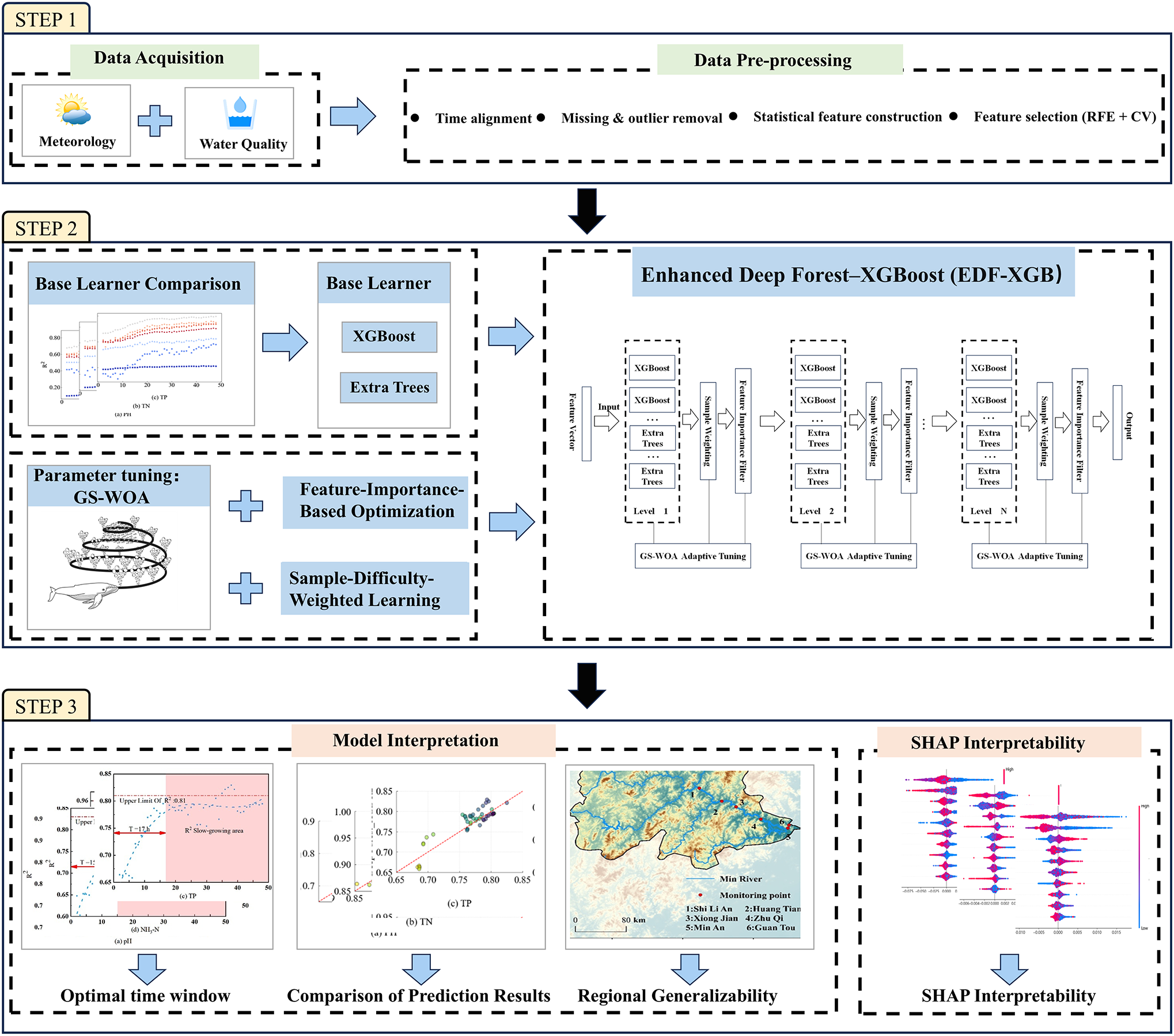
General framework of the Enhanced Deep Forest–XGBoost (EDF–XGB) model for water-quality prediction. The framework includes three stages: (1) Data acquisition and pre-processing, integrating meteorological and water-quality datasets; (2) Model construction and optimization, combining XGBoost and Extra Trees within a Deep Forest cascade and optimized using GS-WOA with feature-importance and sample-weight adjustments; and (3) Model evaluation, regional generalization, and interpretation, assessing predictive performance, spatial transferability, and feature influence via SHAP analysis.
2 Study area and data
2.1 Study area
The Minjiang River Basin (Figure 2) is situated in southeastern China’s Fujian Province and represents the largest independent river system that discharges into the sea in this province (Wang et al., 2021). The main stream extends approximately 562 km, draining a catchment area of approximately 61,000 km2, which accounts for nearly half of Fujian’s total land area. The basin is influenced by subtropical monsoon meteorological conditions, with an annual mean precipitation exceeding 1,000 mm, most of which occurs during the flood season from April to September. Its hydrological regime is largely shaped by monsoonal precipitation, where abundant runoff and frequent floods characterize the summer wet season, whereas flows during the dry season remain comparatively low (Yin et al., 2010). The spatial and temporal variability in hydrological conditions is pronounced, particularly in the Fuzhou section of the main stream, where tidal effects interact with river discharge.
Figure 2
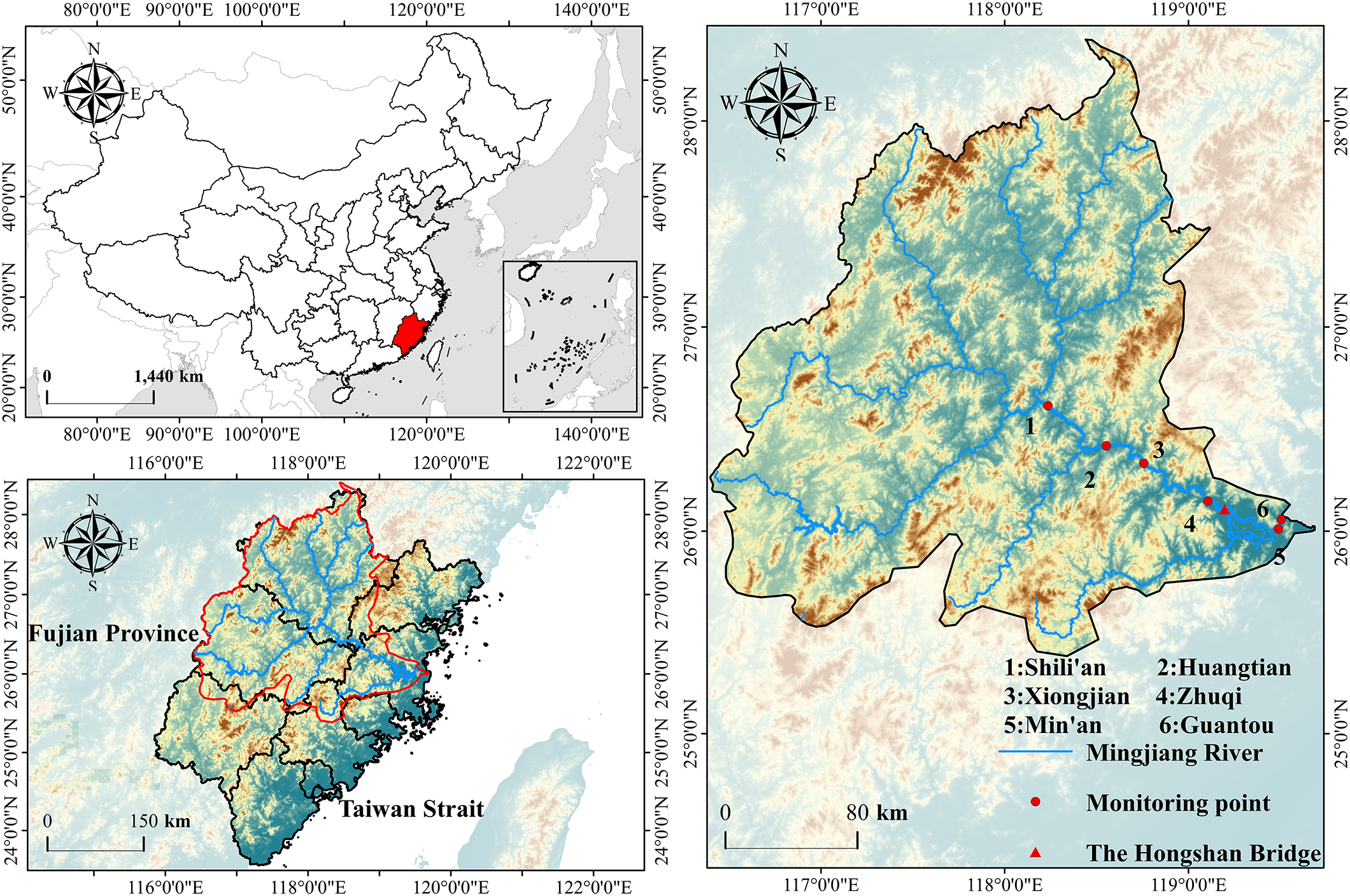
Geographic location of water-quality monitoring stations along the mainstream of the Minjiang River. The figure shows the spatial distribution of six monitoring stations—Shilian’an, Huangtian, Xiongjian, Zhuqi, Min’an, and Guantou—along the Minjiang River. The Hongshan Bridge, marked in yellow, represents the tidal current limit, separating the fluvial reach from the estuarine reach. Fujian Province and its position within southeastern China are also indicated for regional context.
The Minjiang River is dominated by low-mineralized freshwater of bicarbonate-type soft water, primarily derived from carbonate weathering. Major pollution sources include industrial effluents, domestic and medical wastewater, and agricultural runoff, with industrial discharge contributing to approximately 70 percent of the total wastewater load (Kong et al., 2024). According to the Bulletin on the State of Fujian’s Ecological Environment (2021–2023) (Fujian Provincial Local Chronicles Compilation Committee, 2001; Xu, 2022, 2021), the overall surface water quality in Fujian is generally outstanding, with Class I–III waters (as defined in China’s Environmental Quality Standards for Surface Water, GB 3838–2002) accounting for approximately 99% of all monitored sections. However, the proportion of high-quality Class I–II waters declined from 81.4% in 2022 to 68.6% in 2023, indicating the localized deterioration. Notably, the Zhuqi monitoring section in Minhou County has occasionally recorded Class IV, V, or inferior-V water, posing risks because a nearby water intake directly influences domestic water safety (Li et al., 2015).
Therefore, this study selected the Zhuqi section (119°05’28” E, 26°10’00” N), located in the tidal reach, as the focal site for model development and evaluation. Given its ecological and hydrological representativeness, the modeling framework developed here can be extended to other monitoring sites along the Minjiang River main stem for regional generalization and validation. The Hongshan Bridge exhibited the tidal current limit, delineating the transition between the fluvial-dominated upper reach and the tidally influenced estuarine reach of the Minjiang River (Fujian Provincial Local Chronicles Compilation Committee, 2001). Subsequent analyses were performed separately for these two hydrodynamic regions to evaluate spatiotemporal variations in the water quality.
2.2 Data sources
Water quality data were obtained from the National Surface Water Quality Automatic Monitoring System managed by the China National Environmental Monitoring Center. The dataset covered the period from 1 January 2021 to 31 December 2023, with a 4-hour sampling interval. Nine key water quality parameters were adopted as inputs: water temperature (WT), pH, total nitrogen (TN), total phosphorus (TP), ammonia-nitrogen (NH3-N), DO, Permanganate Index (CODMn), turbidity, and electrical conductivity (EC).
Meteorological drivers were retrieved from the ERA5 reanalysis dataset provided by the European Centre for Medium-Range Weather Forecasts (ECMWF). Hourly meteorological records from 1 December 2020 to 31 December 2023 were extracted from 0.25° × 0.25° grid cells involving the main channel monitoring sites. The selected meteorological variables included AT, relative humidity (RH), WS, wind direction (WD), surface temperature (ST), total cloud cover (TCC), and P, which exerted key atmospheric effects on hydrological and biogeochemical processes in the estuarine environment.
2.3 Data pre-processing
To ensure temporal consistency across datasets, hourly meteorological records were synchronized with 4-hourly water quality observations using direct timestamp matching (Reichstein et al., 2019; Shen, 2018). For each water quality sampling time, the corresponding meteorological value was obtained by selecting an hourly record with an identical timestamp. This procedure preserved the original temporal structure of the meteorological drivers while ensuring consistent sampling intervals for subsequent modeling analyses.
Missing observations were handled using a deletion approach to avoid interpolation bias, and outliers were identified and removed using the interquartile range (IQR) method (Dallah et al., 2025; Dong and Peng, 2013). To enhance model performance and introduce additional predictive information under limited monitoring conditions, the hourly meteorological drivers were further processed using statistical sliding window techniques. Through these procedures, structured feature variables suitable for model training were generated from the hourly data (Table 1). For each factor, including AT, RH, WS, WD, ST, total cloud cover, and P, statistical sliding window metrics (e.g., mean, standard deviation, and cumulative values) were determined to capture short-term variability and lagged effects on water quality dynamics.
Table 1
| Original variable (target) | Constructed feature 1 | Constructed feature 2 | Constructed feature 3 | Constructed feature 4 |
|---|---|---|---|---|
| Hourly AT | Mean AT within window | AT at previous timestep | Max AT within window | Min AT within window |
| Hourly WD | Mean WD within window | WD at previous timestep | Std. dev. of WD within window | — |
| Hourly P | Total precipitation within window | Max precipitation within window | Count of hours with P>0.01 mm within window | — |
Meteorological data feature construction after statistical processing.
Feature selection was performed using the recursive feature elimination (RFE) algorithm combined with K-fold cross-validation (RFECV) (Guyon et al., 2002; Kohavi, 1995). This procedure systematically identified the optimal subset of predictors by eliminating redundant or irrelevant variables, thereby improving model stability, interpretability, and computational efficiency.
The dataset from 1 January 2021 to 30 September 2023 was used for model training and preliminary testing, with an 8:2 split between the training and testing sets. The remaining period from 1 October to 31 December 2023 served as an independent validation set to evaluate the model’s generalization capability and predictive robustness.
3 Methodology
3.1 Machine learning framework
3.1.1 Selection of base learners
In this study, to systematically compare the performance of different ensemble algorithms in water quality prediction, several representative base learners were selected, including Support Vector Regression (SVR) (Cortes and Vapink, 1995), Decision Tree (Breiman et al., 1984), Random Forest (Breiman, 2001), Extra Trees Regressor (Geurts et al., 2006), Extreme Gradient Boosting (XGBoost) (Chen and Guestrin, 2016), Light Gradient Boosting Machine (LightGBM) (Ke et al., 2017), and Categorical Boosting (CatBoost) (Prokhorenkova et al., 2018). Figure 3 illustrates that the predictive performance of the algorithms changed substantially with variations in the time window length along the x-axis. Extra Trees consistently achieved the highest R2 values across most water-quality parameters, and its accuracy improved steadily as the time window expanded, demonstrating the strong capability in capturing temporal dependencies. XGBoost followed closely, exhibiting similarly stable and high predictive performance across different window sizes. In contrast, algorithms such as SVR, Decision Tree, and Random Forest exhibited only marginal improvement with increasing window length and remained consistently inferior. These performance differences observed across time windows could provide direct support for selecting Extra Trees and XGBoost as the base learners of the proposed EDF-XGB model, as their robustness and adaptability to varying temporal information substantially strengthened the model accuracy and generalization.
Figure 3
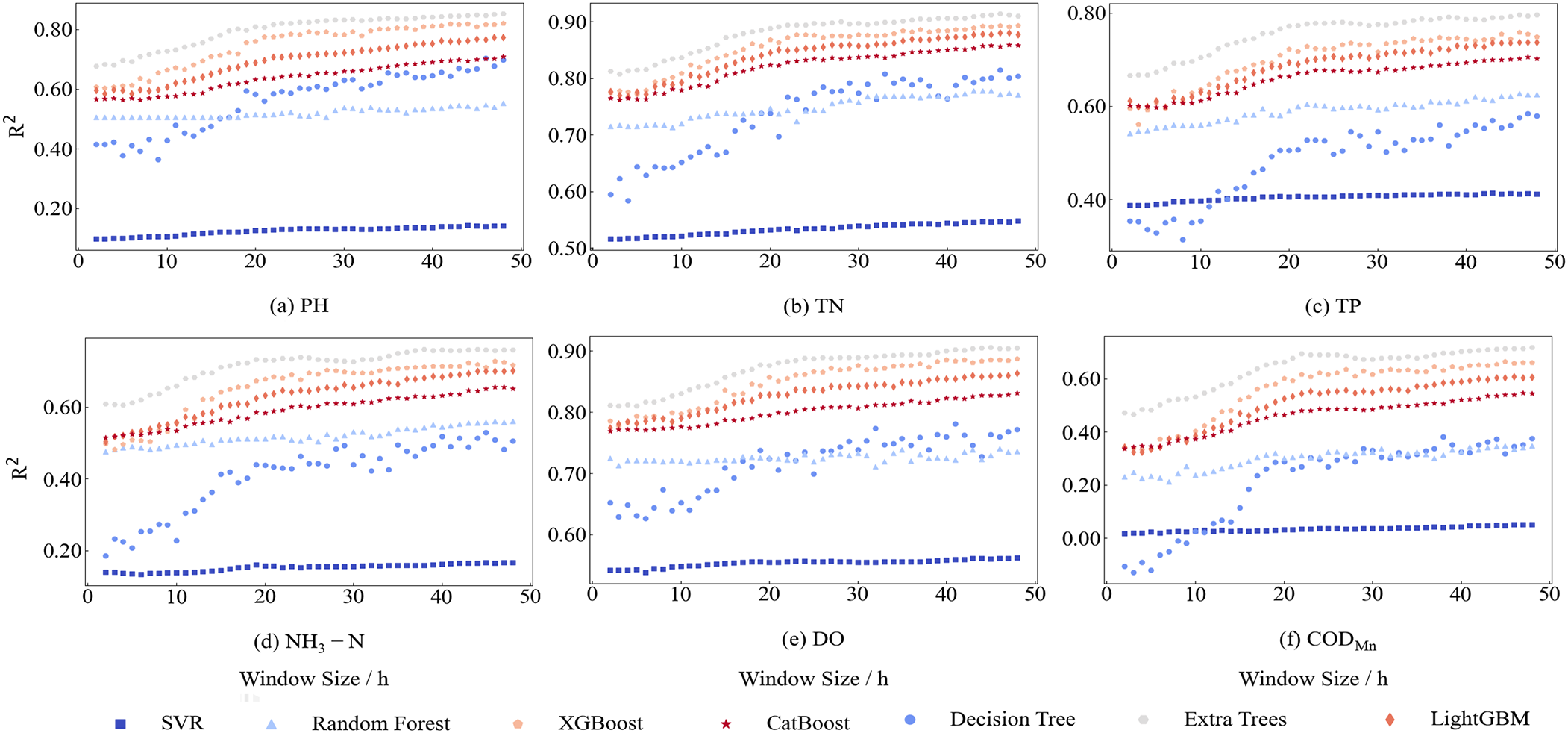
Comparison of water-quality prediction performance among base learners. The figure presents the coefficient of determination (R²) values of seven machine-learning algorithms—SVR, Decision Tree, Random Forest, Extra Trees, XGBoost, LightGBM, and CatBoost—across six water-quality indicators: (a) pH, (b) TN, (c) TP, (d) NH3–N, (e) DO, and (f) CODmn. Results show that ensemble-based learners, particularly XGBoost and Extra Trees, consistently outperform traditional algorithms, demonstrating higher stability and predictive accuracy across varying time windows.
3.1.2 Enhanced deep forest–XGBoost model
DF is a non-neural ensemble learning model composed of multiple layers of cascaded decision tree ensembles, such as Random Forests (RF) and Extra Trees (ETR) (Zhou, 2017). Its main advantage lies in achieving strong predictive performance without complex parameter adjustments. However, DF has several limitations. The model structure is relatively rigid, making it difficult to incorporate time-series information adaptively, and the class vector features may become redundantly expanded during cascading. Therefore, this study introduced a series of incremental optimizations based on the original DF model (Figure 4). These included integrating XGBoost and Extra Trees as base learners to strengthen the model’s ability to represent complex data, employing GS-WOA for adaptive parameter adjustment to enhance performance, and introducing structural improvements through feature-importance-based selection and sample-difficulty weighting to further refine model stability and efficiency. Through these layer-by-layer enhancements, the predictive accuracy and adaptability of the model across different environments were significantly improved.
Figure 4
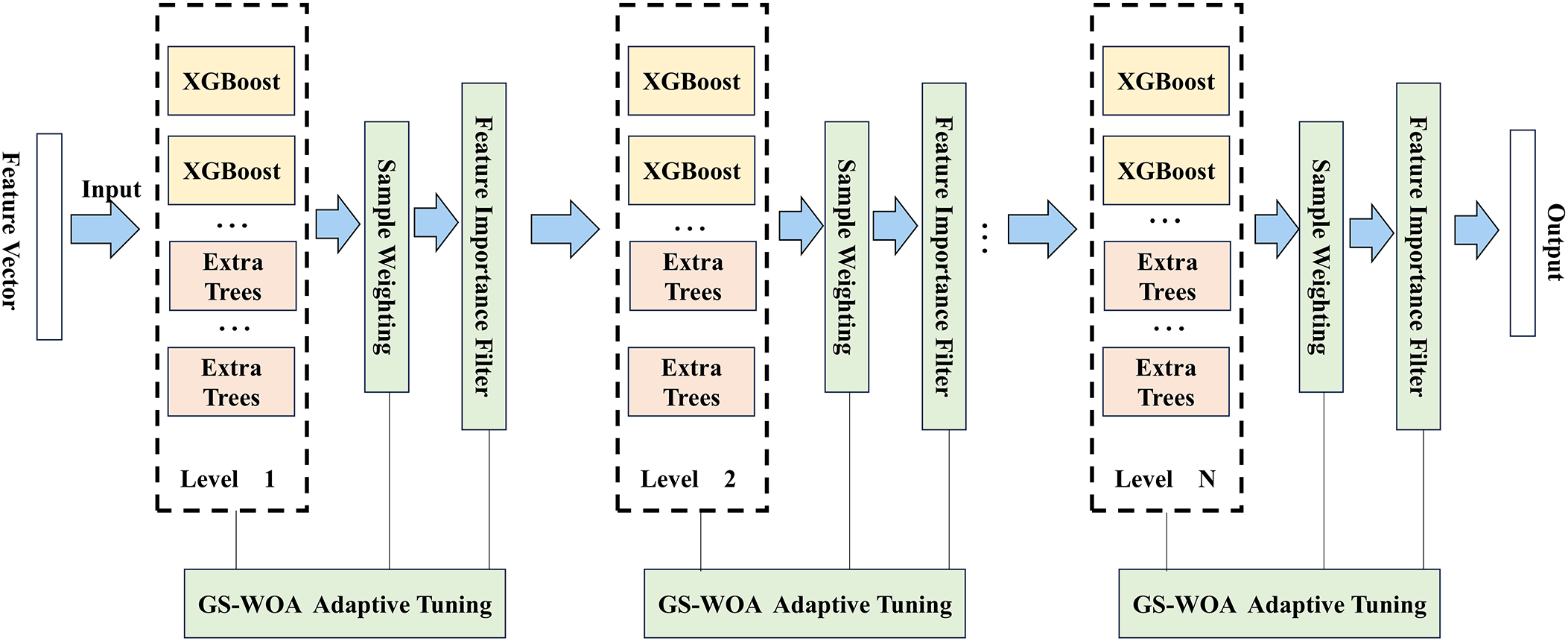
Structural framework of the Enhanced Deep Forest–XGBoost (EDF–XGB) model. The EDF–XGB framework integrates XGBoost and Extra Trees as base learners in a multi-level cascade architecture. At each level, the Global Search Whale Optimization Algorithm (GS-WOA) adaptively tunes model parameters, while feature-importance filtering and sample-difficulty weighting dynamically refine the learning process. The output of each level serves as the input for the next, enabling hierarchical feature representation and improved generalization across complex water-quality dynamics.
3.1.2.1 Integration of XGBoost and Extra Trees Regressor as Base Learners
In traditional DF models, decision-tree-based learners are typically built using Random Forest and Extra Trees (Breiman, 2001). Based on the comparative analysis of base-learner characteristics in the previous section, this study instead employed XGBoost and Extra Trees as the joint base-learner configuration (Chen and Guestrin, 2016). XGBoost incorporates explicit mechanisms for regulating model complexity, including weighted branch evaluation, shrinkage, and subsampling, whereas Extra Trees introduces substantial randomness through fully random split selection. Combining these two learners increases model diversity and provides flexible control over bias–variance trade-offs. Furthermore, XGBoost’s efficient training mechanism is well-suited for large datasets, whereas Extra Trees enhances robustness when dealing with heterogeneous and high-dimensional features (Chen and Guestrin, 2016; Geurts et al., 2006).
Rather than assuming that XGBoost and Extra Trees are inherently superior to the traditional Random Forest and Extra Trees pairing, the application in this study is driven by their complementary algorithmic behaviors. Their suitability for DF architecture was demonstrated empirically through experimental evaluation.
3.1.2.2 Adaptive hyperparameter optimization of deep forest based on the GS-WOA Bio-inspired algorithm
In the standard DF framework, the model performance is generally less sensitive to parameter tuning (Zhou, 2017). However, incorporating XGBoost and Extra Trees as base learners fundamentally changes this behavior. XGBoost contains interacting hyperparameters, including learning rate, tree depth, subsampling ratios, and regularization components, all of which strongly influence the predictive performance (Chen and Guestrin, 2016; Prokhorenkova et al., 2018). Consequently, an effective global optimization strategy is required to obtain stable and well-generalized models.
The hyperparameter search space in this study was high-dimensional, mixed in variable type, and strongly nonlinear, containing continuous, integer, and categorical parameters distributed across a non-convex performance surface. Population-based metaheuristic algorithms are suitable for such conditions because they explore large multimodal spaces without depending on gradient information (Rana et al., 2020). Within this group, the Whale Optimization Algorithm (WOA) is frequently adopted owing to its structural simplicity and competitive continuous-space optimization capability (Mirjalili and Lewis, 2016; Wei et al., 2025).
However, the standard WOA suffers from premature convergence and insufficient exploration in high-dimensional, rugged search spaces. This limitation is evident in comparative analyses. As shown in Table 2, WOA attained reasonable RMSE and R2 values but required significantly longer computation times for most water quality indicators (> 100 s for pH, TN, and NH3-N), reflecting reduced efficiency. Other metaheuristics (e.g., GWO and SSA) exhibit similar limitations. They can achieve acceptable prediction accuracy but impose substantial computational burden.
Table 2
| Parameter | GS-WOA | GWO | SSA | WOA | Bayesian | Random search | |
|---|---|---|---|---|---|---|---|
| time(s) | pH | 30.406 | 100.757 | 108.466 | 65.893 | 4.868 | 13.518 |
| TN | 59.508 | 66.008 | 87.465 | 107.605 | 1.488 | 14.273 | |
| TP | 37.334 | 61.463 | 107.531 | 78.427 | 4.992 | 11.431 | |
| NH3-N | 14.977 | 110.078 | 96.527 | 59.606 | 4.694 | 12.054 | |
| Turbidity | 21.819 | 118.621 | 138.294 | 100.928 | 2.561 | 14.134 | |
| DO | 50.109 | 83.044 | 112.100 | 77.354 | 1.880 | 10.319 | |
| CODMn | 34.340 | 59.578 | 121.995 | 122.331 | 3.220 | 13.989 | |
| RMSE | pH | 0.070 | 0.067 | 0.069 | 0.067 | 0.068 | 0.068 |
| TN | 0.073 | 0.075 | 0.074 | 0.075 | 0.079 | 0.075 | |
| TP | 0.007 | 0.007 | 0.007 | 0.007 | 0.007 | 0.007 | |
| NH3-N | 0.015 | 0.015 | 0.015 | 0.015 | 0.016 | 0.015 | |
| Turbidity | 6.565 | 6.563 | 6.558 | 6.557 | 6.646 | 6.594 | |
| DO | 0.433 | 0.421 | 0.428 | 0.434 | 0.434 | 0.425 | |
| CODMn | 0.187 | 0.188 | 0.185 | 0.183 | 0.188 | 0.183 | |
| R² | pH | 0.846 | 0.858 | 0.846 | 0.855 | 0.851 | 0.852 |
| TN | 0.945 | 0.942 | 0.943 | 0.941 | 0.935 | 0.942 | |
| TP | 0.815 | 0.818 | 0.814 | 0.817 | 0.820 | 0.818 | |
| NH3-N | 0.670 | 0.668 | 0.668 | 0.678 | 0.663 | 0.669 | |
| Turbidity | 0.427 | 0.427 | 0.428 | 0.428 | 0.412 | 0.421 | |
| DO | 0.892 | 0.898 | 0.894 | 0.891 | 0.892 | 0.896 | |
| CODMn | 0.742 | 0.738 | 0.745 | 0.751 | 0.738 | 0.752 |
Performance comparison of GS-WOA, GWO, SSA, WOA, Bayesian, and Random Search in hyperparameter optimization for water-quality prediction.
In contrast, although Bayesian Optimization and Random Search have been widely adopted for hyperparameter tuning, they are less effective in this context. Bayesian Optimization struggles with the scalability in high-dimensional and heterogeneous parameter spaces. The Gaussian-process surrogate becomes unstable or inaccurate, and the exploitation-biased search strategy fails to navigate highly multimodal landscapes. Random Search, which is simple, is intrinsically inefficient for mixed-type high-dimensional problems and cannot ensure adequate coverage of the search space. This issue becomes more severe when EDF-XGB introduces dynamic weighting and sample difficulty mechanisms that alter the loss landscape during training. Additionally, both Bayesian Optimization and Random Search lack population diversity, making them poorly suited for modeling the complex, evolving interactions between hyperparameters in the hierarchical DF–XGB structure.
To overcome these limitations, this study employed the Global Search Whale Optimization Algorithm (GS-WOA), an enhanced variant of the standard WOA (Liu et al., 2020). GS-WOA incorporates adaptive control coefficients, diversified position-update rules, and neighborhood perturbations to strengthen global exploration and mitigate premature stagnation. As shown in the empirical comparison in Table 2, GS-WOA delivers an accuracy comparable to or exceeding that of the other algorithms while achieving the shortest computation time across nearly all water quality indicators. This balanced combination of accuracy, stability, and efficiency, along with its robustness under dynamic weighting and difficulty-based sample adjustments, renders GS-WOA the most suitable optimizer for the EDF–XGB framework.
The adaptive weighting mechanism is defined by the time‐varying weight function in Equation (1), and the corresponding position updating strategy is given in Equation (2).
In the equation, represents the position vector of the current global best solution, while denotes the position vector of an individual whale at iteration . is the contraction coefficient controlling the search range, and is the weight vector used to perturb the optimal solution randomly. denotes the current iteration number; is a random number within the range [–1,1]; and measures the distance between the current search agent and the selected target agent. represents the maximum number of iterations.
The variable-spiral position update strategy is defined by the position updating rule and the spiral parameter, as shown in Equation (3)
In the equation, b represents the spiral parameter.
The optimal-neighborhood perturbation mechanism is formulated as shown in Equation (4), and the update rule for the global best position is given in Equation (5).
If the fitness condition is satisfied, the global best position is updated as:
In this equation, and are random numbers uniformly distributed within the range [0,1]; represents the newly generated position; and denotes the fitness value corresponding to position .
In summary, GS-WOA attains a coordinated balance between global exploration and local exploitation. It accelerates convergence and improves optimization accuracy while maintaining stability and scalability in high-dimensional and complex search spaces. These characteristics enable GS-WOA to provide superior optimization efficiency and stronger generalization performance when applied to the adaptive hyperparameter tuning of the DF model.
3.1.2.3 Structural enhancement of deep forest based on feature-importance optimization
In any deep learning framework, the quality of input features directly shapes the overall model performance. The DF model adopts a cascading strategy in which each layer’s output is concatenated with the original input features and then transmitted to the next layer. However, this mechanism does not consider the unequal contributions of individual features. To address this limitation, a feature importance-guided evaluation mechanism was incorporated into the DF framework, and GS-WOA was employed to adaptively optimize the feature retention threshold across layers. This integrated approach strengthened information utilization efficiency and ensured that the most relevant and influential features were preserved for subsequent learning.
Specifically, the proposed feature-importance module combined each layer’s output with the original features and then applied an importance-scoring procedure based on the information gain or model weight analysis to quantify the predictive contribution of each feature. These importance scores were used to rank the features. Instead of forwarding all the features to the next layer, only the top-ranked and most informative subsets were selected. This filtering not only reduced the feature dimensionality but also ensured that the most predictive features were retained for the subsequent layers.
The primary objective of this strategy was to enhance computational efficiency, reduce model complexity, and mitigate the overfitting risk associated with high-dimensional feature spaces. By repeating this process across multiple layers, DF achieved progressively more focused and precise feature learning at each stage, thereby improving the overall predictive accuracy.
3.1.2.4 Structural enhancement of deep forest based on sample-difficulty weighting
When optimizing the DF model, it is crucial to consider the varying learning difficulties of individual samples. The original DF framework assigns uniform weights to all samples, an approach that neglects heterogeneity in data complexity and learning contribution. To address this issue, a dynamic sample-weighting mechanism was introduced to adaptively adjust each sample’s importance according to its learning difficulty.
Specifically, the samples exhibiting larger prediction errors than the mean were classified as difficult samples and assigned higher weights. These dynamically updated weights were then passed to the next DF layer, enabling the model to focus more strongly on complex and informative samples while reducing overfitting to easy cases. To further refine this adaptive weighting process, GS-WOA was incorporated for the joint global optimization of sample weights and model parameters. Through the iterative adjustment of weighting coefficients based on performance feedback, GS-WOA maintained a balanced learning process between difficult and non-difficult samples. This approach strengthened the model’s capability to recognize and capture complex data patterns and improved its generalization across multiple datasets. Meanwhile, it balanced the attention allocated to difficult and non-difficult samples, thereby enhancing overall predictive performance.
3.2 Time-varying window
The configuration of the time window was carefully examined to investigate the influence of meteorological conditions on water quality predictions. Different time-window lengths () were applied to all meteorological drivers, and a unified statistical procedure was adopted to pre-process the data. WT and EC were selected as input features for the water quality prediction model. The coefficient of determination (R2) was adopted as the performance metric to identify the time window size that provided the highest prediction accuracy.
Assume that the meteorological variable consists of time-series measurements. The time series can be represented as: , where represents the measurement of meteorological variable at the time step. Similarly, let denote the water quality variables measured 4 h, forming another time series: . where represents the water quality measurement of variable at the time step. If the model aims to predict at time, the corresponding meteorological features from the preceding steps can be expressed as, where denotes the time window length.
For single-factor prediction, historical observations of all meteorological factors within the selected window were pre-processed using the same statistical methods. These features with WT and EC, were then adopted as the model inputs to predict the target water quality variable at the next time step . The overall construction framework of the time window configuration is illustrated in Figure 5.
Figure 5
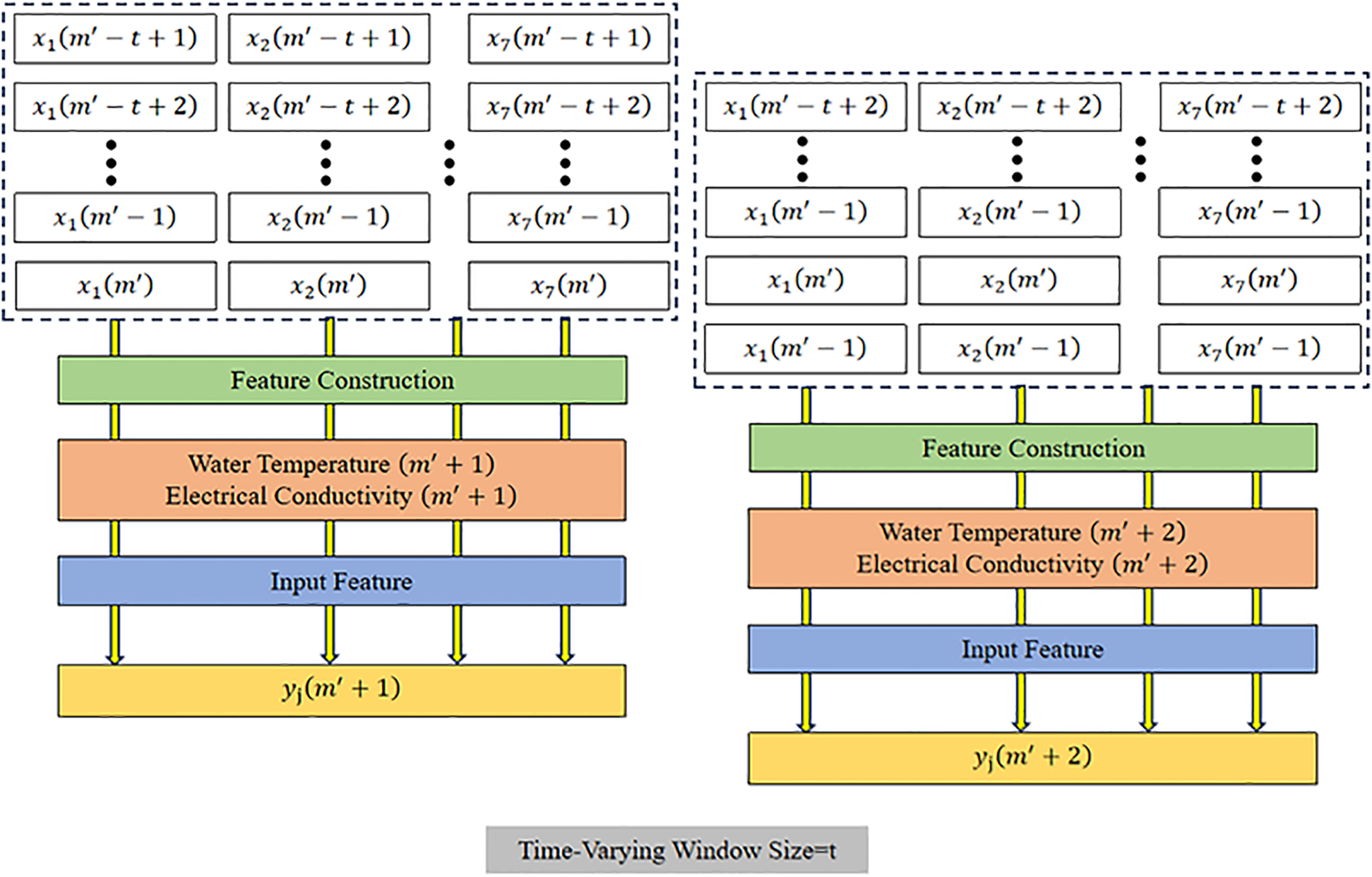
Time-varying window structure for dynamic feature construction. This diagram illustrates the design of a sliding statistical window with a variable size (t), used to capture short-term temporal dynamics of water-quality parameters. For each prediction step (m′ + 1, m′ + 2,…), meteorological and hydrological variables (e.g., WT, EC) within the corresponding window are aggregated through feature construction to form the input features. This approach enables adaptive learning of time-dependent patterns and improves the model’s responsiveness to rapidly changing environmental conditions.
3.3 Model performance evaluation metrics
Water quality prediction can be formulated as a regression task. Therefore, the Root Mean Square Error (RMSE) and the Coefficient of Determination (R2) are generally adopted as the primary evaluation metrics. RMSE represents the magnitude of the deviation between the predicted and observed values, where lower values correspond to higher predictive accuracy. Additionally, R2 reflects the model’s goodness of fit, with values approaching 1 indicating a stronger explanatory power and enhanced fitting capability. Accordingly, the Root Mean Square Error (RMSE) and the coefficient of determination (R²) are calculated using Equations (6) and (7), respectively.
where denotes the observed (actual) value, represents the predicted value, is the mean of , and indicates the total number of samples in the test set.
3.4 SHAP interpretability analysis
SHAP, grounded in cooperative game theory, provides a mathematically rigorous framework for quantifying the contribution of each input feature to model predictions (Lundberg and Lee, 2017). As demonstrated by Chen et al (Chen et al., 2025), it enables transparent assessment of how individual variables influence model outputs by decomposing each prediction into additive attribution values.
For a given prediction, the contribution of feature is measured by its Shapley value , which represents the average marginal improvement in the model output when is added to all possible subsets of the remaining features. Formally, the Shapley value is defined as shown in Equation (8). (Lundberg and Lee, 2017):
In the equation, is the full set of input features, denotes the model output, and is the sample restricted to the subset .
In this study, SHAP served as both an interpretability tool and a feature-selection aid. For each layer of the proposed ensemble architecture, SHAP values were computed for all base learners using the TreeSHAP algorithm, which provides exact and computationally efficient Shapley value estimation for tree-based models (Lundberg et al., 2019). The SHAP values from all base learners within the same layer were then averaged to derive layer-level feature attributions, thereby improving robustness and reducing model-specific variability. Beyond quantifying relative importance, SHAP also provides directional interpretability: a positive SHAP value indicates that a feature increases the predicted concentration of a water-quality parameter relative to the model baseline, whereas a negative value implies a suppressing effect (Aldrees et al., 2024). The magnitude of the SHAP value reflects the strength of this influence, with larger absolute values denoting a more substantial contribution, regardless of direction. This directional and magnitude-based interpretation enables the model not only to identify which meteorological drivers matter most but also to reveal how high or low feature values push predictions upward or downward in physically meaningful ways.
This multi-level SHAP analysis provided a transparent and quantitatively robust interpretation of how meteorological drivers shape the multi-indicator water-quality dynamics within the proposed modeling framework. Finally, the layer-wise SHAP values were aggregated across all layers to obtain the overall importance and directional influence of each meteorological driver on water-quality predictions.
4 Results
4.1 Performance analysis of the EDF-XGB model
As shown in Table 3 and Figure 6, both the DF and EDF-XGB models exhibited an overall improvement in predictive performance across different time window lengths for indicators such as pH, TN, and TP, eventually reaching a steady plateau. This pattern indicates that both models effectively captured the temporal dynamics of water quality parameters. Notably, the EDF-XGB model consistently outperformed the DF model with respect to the R2 metric.
Table 3
| Parameter | R² | RMSE | ||
|---|---|---|---|---|
| DF | EDF-XGB | DF | EDF-XGB | |
| pH | 0.85 | 0.90 | 0.054 | 0.052 |
| TN | 0.92 | 0.96 | 0.090 | 0.072 |
| TP | 0.80 | 0.81 | 0.007 | 0.007 |
| NH3-N | 0.77 | 0.83 | 0.014 | 0.013 |
| DO | 0.91 | 0.93 | 0.420 | 0.380 |
| CODMn | 0.72 | 0.78 | 0.160 | 0.150 |
| Turbidity | 0.56 | 0.65 | 5.500 | 5.200 |
Comparison of R2 and RMSE Values between DF and EDF-XGB.
Figure 6
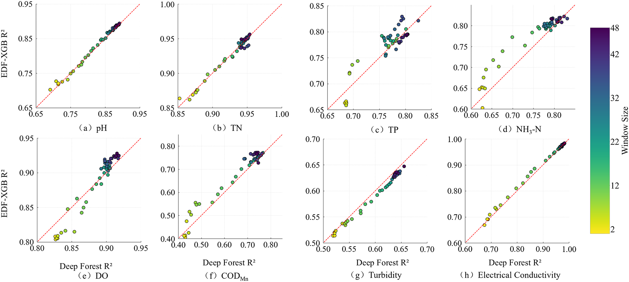
Comparison of R² values between DF and EDF–XGB models. The figure compares the coefficient of determination (R²) values of the traditional Deep Forest and the proposed EDF–XGB model across eight water-quality indicators: (a) pH, (b) TN, (c) TP, (d) NH3–N, (e) DO, (f) CODmn, (g) Turbidity, and (h) Electrical Conductivity. Each point represents the model performance under different time-varying window sizes. Most points lie above the 1:1 line, indicating that EDF–XGB consistently outperforms Deep Forest in predictive accuracy across varying temporal resolutions.
In particular, the EDF-XGB model yielded substantial gains in predictive accuracy for pH and TN, where R2 increased from approximately 0.89 to above 0.90 for pH and from 0.92 to approximately 0.96 for TN. These improvements highlight the enhanced capacity of the model to represent and forecast the underlying temporal evolution of these parameters. Comparable performance enhancements were also observed for DO, ammonia nitrogen (NH3-N), and CODMn.
However, in the prediction tasks for NH3-N and CODMn, the EDF-XGB model demonstrated a more pronounced advantage over the standard DF model, with R2 values aligning more closely with the ideal 1:1 reference line (y = x). This outcome suggests that incorporating XGBoost as a base learner substantially strengthens the model’s ability to capture complex, nonlinear, and dynamic patterns. In contrast, for turbidity, the EDF-XGB model showed slightly inferior performance relative to the standard DF model, potentially because of the higher stochasticity and spatial variability associated with this parameter.
4.2 Regional generalization of the EDF-XGB model
To assess the generalization capability of the improved EDF-XGB model under varying geographical and hydrodynamic conditions, a comparative analysis was conducted using representative monitoring stations distributed along the main stem of the Minjiang River. The evaluation focused on the model’s predictive skill across two hydrodynamically distinct regions: the upstream reaches located above the tidal current limit and the downstream reaches located below this limit, where tidal influence becomes progressively more pronounced.
Upstream reaches situated inland and largely unaffected by tidal processes generally exhibit stable environmental settings, recognizable water quality patterns, and minimal anthropogenic or industrial perturbations. Such conditions create a favorable context for prediction models driven primarily by meteorological inputs. In this study, the stations at Zhuqi, Xiongjian, Huangtian, and Shilian’an were selected as representative upstream sites.
As presented in Table 4, the EDF-XGB model demonstrated strong predictive performance across the upstream reaches. Most water quality indicators yielded R2 values exceeding 0.9, reflecting the high accuracy and strong reliability of the model for non-tidal water quality variability.
Table 4
| Evaluation metric | Water quality parameter | Upstream of the tidal current limit | Downstream of the tidal current limit | ||||
|---|---|---|---|---|---|---|---|
| Shilian’an | Huangtian | Xiongjiang | Zhuqi | Guantou | Min’an | ||
| R2 | WT | 0.9952 | 0.9905 | 0.9946 | 0.9934 | 0.9902 | 0.9960 |
| pH | 0.9007 | 0.9057 | 0.8611 | 0.9014 | 0.7530 | 0.8745 | |
| TN | 0.9363 | 0.9713 | 0.9883 | 0.9615 | 0.7857 | 0.9083 | |
| TP | 0.9143 | 0.9250 | 0.9446 | 0.8332 | 0.4336 | 0.6595 | |
| NH3-N | 0.9383 | 0.9649 | 0.8069 | 0.8328 | 0.5330 | 0.7478 | |
| DO | 0.9277 | 0.9361 | 0.9687 | 0.9324 | 0.9637 | 0.9626 | |
| CODMn | 0.6753 | 0.7132 | 0.6521 | 0.7927 | 0.4427 | 0.4650 | |
| Turbidity | 0.9158 | 0.8796 | 0.8521 | 0.6789 | 0.2386 | 0.6582 | |
| EC | 0.8980 | 0.9408 | 0.9944 | 0.9836 | 0.5016 | 0.5978 | |
| RMSE | WT | 0.4423 | 0.5483 | 0.4306 | 0.4641 | 0.4011 | 0.3907 |
| pH | 0.0519 | 0.0879 | 0.0730 | 0.0512 | 0.2217 | 0.1010 | |
| TN | 0.0936 | 0.0577 | 0.0374 | 0.0729 | 0.6402 | 0.1930 | |
| TP | 0.0049 | 0.0033 | 0.0028 | 0.0064 | 0.0326 | 0.0342 | |
| NH3-N | 0.0199 | 0.0129 | 0.0197 | 0.0130 | 0.0940 | 0.0471 | |
| DO | 0.3419 | 0.5138 | 0.3748 | 0.3754 | 0.2642 | 0.2584 | |
| CODMn | 0.1550 | 0.1981 | 0.1968 | 0.1514 | 0.8599 | 0.6205 | |
| Turbidity | 2.7910 | 2.4252 | 1.6199 | 5.2666 | 80.4808 | 45.2534 | |
| EC | 15.0338 | 10.5443 | 2.9962 | 5.4945 | 5882.0972 | 3127.3050 | |
Comparison of the predicted performance of each water quality monitoring site in the main stream of the Min Rive.
In contrast, downstream tidal reaches are characterized by periodic tidal oscillations and considerable anthropogenic disturbances associated with urbanization (Malli et al., 2022; Xu et al., 2013). These interacting processes introduce substantial complexity into water quality dynamics and reduce predictive accuracy relative to upstream sections. In this study, the Guantou and Min’an stations served as representative monitoring sites in the tidal region.
A detailed cross-parameter comparison revealed evident spatial heterogeneity in model performance. The predictions for WT and DO showed exceptionally high accuracy, with WT achieving an R2 value approaching 1.0 and DO producing strong results (R2 ≈ 0.96), occasionally outperforming upstream predictions. The indices of pH and TN remained well-predicted but displayed evident inter-station differences. At Min’an, the R2 values for pH and TN reached 0.87 and 0.91, respectively, whereas at Guantou, they declined to 0.75 and 0.79, respectively. For TP, NH3-N, CODMn, Turbidity, and EC, the predictive capability decreased notably in the tidal zone, as manifested by the reduced R2 values and elevated RMSE levels relative to the upstream sites.
Overall, these findings demonstrated that the EDF-XGB model adapted robustly to relatively stable hydrological environments but experienced reduced predictive skill under strong tidal forcing and pronounced anthropogenic disturbance. This contrast underscores the need for future research to incorporate hydrodynamic coupling and spatial heterogeneity when developing predictive frameworks for estuarine and tidal systems.
4.3 SHAP-based feature contribution analysis
Model interpretability is particularly critical in environmental modeling, especially when examining the coupling between high-dimensional meteorological variables and water quality indicators. Identifying the contribution of individual input variables to model predictions not only supports model refinement but also provides a scientific basis for environmental and ecological management. In this section, the SHAP method was used to quantify each feature’s contribution to the model output, and visualization techniques were applied to clarify explanatory mechanisms and influence pathways of key variables.
As illustrated in Figure 7, the feature-importance heatmap presented the normalized mean absolute SHAP values for all predictors, where darker shading indicates a stronger influence on model outcomes. The results revealed that WT and EC consistently ranked as the two most influential drivers in nearly all prediction tasks. For example, in the TP prediction, their normalized SHAP values reached 1.0 and 0.96, respectively. Several meteorological variables, including AT, RH, and ST, also contributed substantially, particularly to dynamic indicators such as ammonia nitrogen (NH3-N), DO, and CODMn. Specifically, for NH3-N, the average relative humidity within the time window (RH_AVG) contributed 0.38, whereas for CODMn, the average surface temperature (ST_AVG) and maximum air temperature (AT_MAX) contributed 0.49 and 0.43, respectively. In contrast, the precipitation-related variables (P) exhibited generally low global SHAP values, indicating a limited influence on most prediction targets.
Figure 7
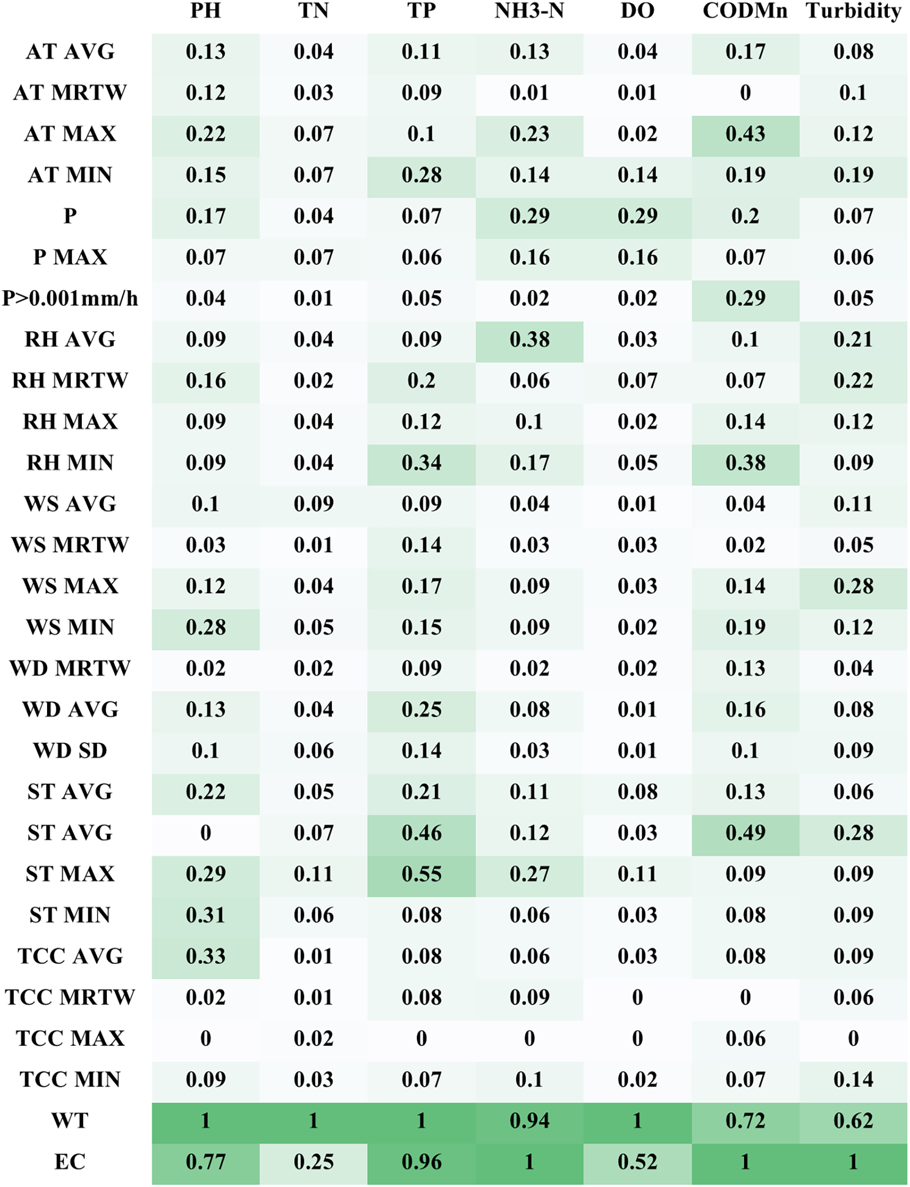
Feature-importance heatmap of meteorological and hydrological variables for water-quality prediction. The heatmap presents the normalized feature-importance values of multiple meteorological and hydrological variables across six key water-quality indicators (pH, TN, TP, NH3–N, DO, and CODmn). Darker shades indicate stronger contributions to prediction accuracy. Among all factors, water temperature (WT) and electrical conductivity (EC) exhibit consistently high importance, followed by air temperature (AT), relative humidity (RH), and surface temperature (ST), highlighting the dominant influence of thermodynamic and atmospheric variables on estuarine water quality.
Figure 8 further illustrates the direction and magnitude of the influence of each feature on the model outputs. Overall, WT and EC dominated the contribution landscape across multiple parameters, and the color gradient (red for high feature values and blue for low) highlighted their substantial roles in shaping predictions. For DO, high WT values produced a pronounced negative SHAP effect, indicating that elevated temperatures reduced the predicted DO concentrations, which is consistent with established physicochemical principles, such as the temperature dependence of gas solubility. Furthermore, meteorological variables related to temperature and humidity exerted a meaningful influence on the dynamics of NH3-N and CODMn, reaffirming the strong sensitivity of water quality evolution processes to external meteorological fluctuations.
Figure 8
![Seven SHAP value diagrams illustrate the impact on model outputs for different environmental variables: (a) pH, (b) TN, (c) TP, (d) \[NH_3\]-H, (e) DO, (f) COD_Mn, and (g) Turbidity. Each plot shows various features on the y-axis and SHAP value on the x-axis, with color gradients indicating feature values from low (blue) to high (red).](https://www.frontiersin.org/files/Articles/1730509/xml-images/fmars-12-1730509-g008.webp)
SHAP summary plots illustrating feature contributions across water-quality indicators.The SHAP summary plots display the impact of meteorological and hydrological features on the prediction of six water-quality parameters: (a) pH, (b) TN, (c) TP, (d) NH₃–N, (e) DO, (f) COD, and (g) Turbidity. Each point represents a single observation, with color indicating the feature value (red for high, blue for low). The horizontal spread reflects the magnitude and direction of the feature’s contribution to model output. Overall, water temperature (WT) and electrical conductivity (EC) are the most influential variables, followed by surface temperature (ST), relative humidity (RH), and precipitation (P), confirming their dominant roles in estuarine water-quality dynamics.
5 Discussion
5.1 Comparative analysis of model performance
The proposed EDF-XGB demonstrated substantial improvements in predictive performance compared with the traditional DF model across most water quality indicators (Table 3; Figure 6). Specifically, for relatively stable biochemical parameters (e.g., pH, TN, and DO) and more dynamic indicators (e.g., ammonia nitrogen (NH3-N) and CODMn), EDF-XGB achieved higher coefficients of determination (R2) and lower root mean square errors (RMSE). These consistent performance gains validate the effectiveness of the model optimization strategies. One noteworthy exception was turbidity, for which predictive improvement was unstable. In several cases, the standard DF model even outperformed the more structurally complex EDF-XGB, highlighting the heterogeneous responsiveness of different water quality parameters to model architecture.
The overall superiority of EDF-XGB aligns with the findings reported in numerous previous studies. Several studies have confirmed that gradient boosting decision tree (GBDT) algorithms, represented by XGBoost, generally outperform traditional ensemble methods such as Random Forests when handling nonlinear, high-dimensional environmental data (Lu and Ma, 2020; Yan et al., 2024). For instance, Lu and Ma (2020) compared multiple machine-learning models for river water quality prediction and found that XGBoost achieved higher accuracy and greater stability than both Random Forest and Support Vector Regression (Lu and Ma, 2020). However, the difficulty in predicting turbidity has been emphasized in previous studies. Aslam et al., (2022) suggested that turbidity indicators driven by physical processes, such as rainfall-runoff and sediment resuspension, tended to show strong randomness, impulsiveness, and event-driven characteristics, which created substantial challenges for purely data-driven models (Aslam et al., 2022). Even hybrid deep learning frameworks may face accuracy limitations when forecasting highly dynamic variables (Barzegar et al., 2020). These observations closely corresponded with the unstable turbidity prediction performance observed for EDF-XGB in this study.
The performance improvement of EDF-XGB can be attributed to the complementary roles of the selected base learners and the optimized cascaded structure. In the proposed framework, XGBoost is embedded into the DF architecture to introduce gradient-boosting–based iterative refinement, in which successive trees emphasize the residual information from preceding iterations. This mechanism strengthens the model’s capacity to learn complex and nonlinear relationships among influential variables such as NH3-N and CODMn. Meanwhile, Extra Trees provide substantial stochasticity through randomized feature selection and randomly generated split points, increasing model diversity and supplying alternative representations of the predictor space. By integrating learners with distinct learning behaviors, the EDF-XGB framework expands the expressiveness of the cascaded structure and allows a more flexible balance between approximation capacity and variability. This ensemble design consequently enhances the adaptability of the DF architecture without suggesting its inherent superiority over all traditional base learner configurations.
The difficulty in predicting turbidity arises from the intrinsic characteristics of the data generation process. Turbidity fluctuations are frequently triggered by short-term, high-intensity events, such as heavy rainfall or sediment resuspension, which appear as sparse, high-amplitude “pulse signals” within time-series data. For a high-capacity and strongly nonlinear model, such as EDF-XGB, the limited availability of such events in the training dataset may lead to their misinterpretation as noise or result in overfitting, thereby reducing the generalization performance on unseen data. In contrast, the simpler and more randomized DF model, which cannot fit the training signals as aggressively, may exhibit greater robustness to these noisy, event-driven fluctuations.
These findings provide practical guidance for model selection and application in water quality prediction. For indicators governed primarily by biochemical processes with smoother or periodic variations (e.g., DO, TN, and pH), the EDF-XGB model represents a reliable option for achieving high-accuracy predictions owing to its strong nonlinear fitting capacity and ability to uncover deep interactions between meteorological and water quality features. However, for event-driven indicators such as turbidity, which are shaped by physical disturbances, relying exclusively on a complex black-box model may not yield optimal results. Therefore, future research should consider fine-grained matching strategies between models and indicator characteristics. A promising direction is the development of hybrid models, in which the EDF-XGB framework is augmented with event-based physical descriptors such as cumulative rainfall, rainfall intensity, and flow rate variation. By explicitly incorporating these event-related features into the model input, the algorithm can learn event response patterns rather than only fitting numerical data. This approach can maintain high predictive accuracy while improving the model’s explanatory capability and physical interpretability for forecasting sudden water quality events.
5.2 Sensitivity analysis and optimization of input time window
The results of this study revealed a nonlinear relationship between model performance and the size of the input time window (Figure 9). For all examined water quality indicators, the predictive accuracy of the EDF-XGB model measured by the coefficient of determination (R2) generally followed a pattern of rapid growth followed by gradual stabilization as the input window was extended from a short to a long duration. This pattern suggests the presence of an “information saturation point” in the model learning process, indicating that an optimal temporal window exists beyond which additional historical data can provide diminishing marginal benefits or may even introduce noise. A comparison between the EDF-XGB and DF models under their respective optimal windows (Table 1) further confirmed that EDF-XGB demonstrated superior capability in capturing temporal dependencies, as reflected by its consistently higher R2 and lower RMSE values across most indicators.
Figure 9
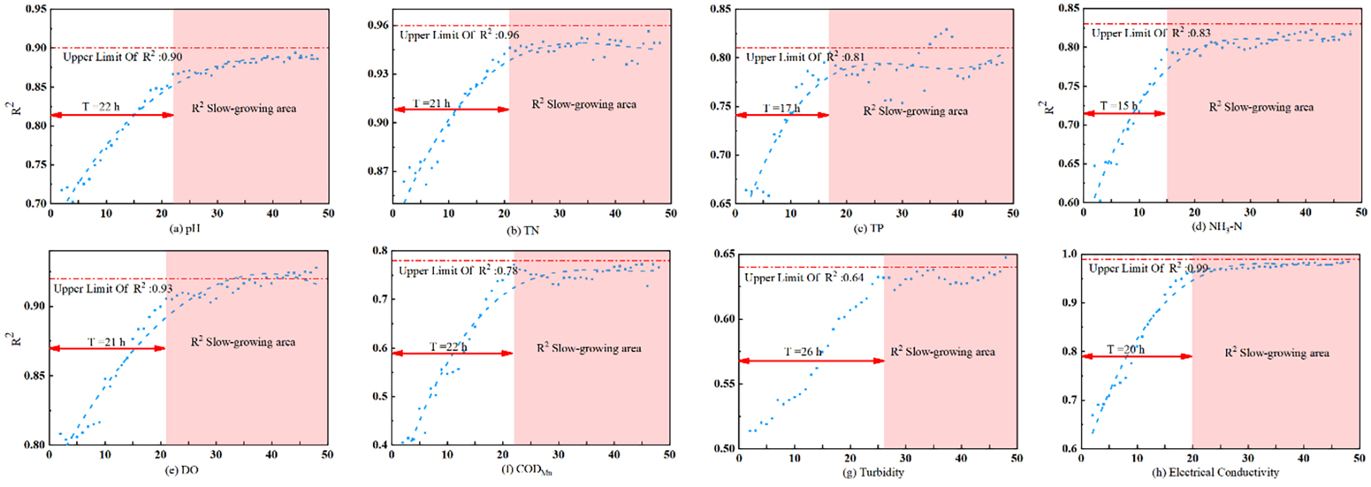
R2 trends of the EDF–XGB model under different time-varying window sizes.The figure illustrates how the coefficient of determination (R2) of the EDF–XGB model varies with different time-varying window sizes for eight water-quality indicators: (a) pH, (b) TN, (c) TP, (d) NH₃–N, (e) DO, (f) COD, (g) Turbidity, and (h) Electrical Conductivity. The red arrows mark the optimal time-varying window size (T*), determined as the inflection point beyond which R² growth becomes slow. For relatively stable physicochemical indicators such as pH, TN, TP, and DO, a moderate window length (≈21–22 h) sufficiently captures their primary temporal patterns. In contrast, NH₃–N and COD exhibit stronger periodic and delayed responses, driven by upstream pollutant discharge and biochemical degradation, requiring longer windows to achieve optimal prediction accuracy.
The observed “rise–then–plateau” behavior could be common in machine learning applications involving environmental time-series prediction. Selecting an appropriate input window length (or lag time) is a critical step in model construction because it directly affects the model’s capacity to represent the system dynamic memory. If the window is too short, the model receives insufficient prior information to infer current conditions, resulting in a high bias. Conversely, an excessively long window may incorporate outdated or weakly relevant information, increasing variance and computational cost (Mosavi et al., 2018). When applying an LSTM model to water quality prediction, Song et al. (2021) identified an optimal time step through experimentation and emphasized that proper input window selection is essential for reliable model performance (Song et al., 2021). The findings of the present study are consistent with these perspectives, confirming that no single universal window size is suitable for all indicators, with the variables requiring a customized configuration aligned with their temporal dynamics.
The differences in the optimal window lengths across water quality parameters arise from their distinct evolutionary mechanisms and response time scales. For pH, TN, and DO with variations significantly governed by diurnal, weekly, or seasonal cycles associated with solar radiation and temperature, the dynamics were relatively smooth. Thus, a moderate window length (approximately 21–22 h in this study) was sufficient to capture primary patterns. For NH3-N and CODMn, both periodic and delayed processes, such as pollutant discharge and biochemical degradation, play important roles, necessitating a slightly longer window (approximately 15–27 h) to capture these lagged effects. For TP, the model exhibited the strongest sensitivity to window size, reflecting TP’s complex transport and transformation mechanisms. In natural water systems, TP is often associated with suspended particulate matter, and its abrupt concentration changes are tightly linked to short-term rainfall-runoff events and sediment resuspension. A window that is too short fails to capture pre-event accumulation effects during dry periods, whereas an excessively long window can smooth out critical flood peaks, eventually degrading model performance.
This analysis provides several practical insights for the deployment of data-driven water quality prediction models. First, the time window length should be recognized as a key hyperparameter that requires systematic optimization determined individually for each target variable through cross-validation rather than using a single empirical value. Second, for parameters such as TP and turbidity, which are highly sensitive to window variation and influenced by multi-scale processes, a single optimal window may remain insufficient. Future model developments could incorporate a multi-scale input mechanism, enabling the model to extract information from both short-term fluctuations and long-term trends, thereby improving predictive robustness and the representation of hydrodynamic process dynamics.
5.3 Regional generalization
The regional generalization capability of a model serves as a fundamental criterion for evaluating its applicability under diverse environmental conditions. The comparative analysis between the upstream (non-tidal) and downstream (tidal) reaches of the Minjiang River revealed pronounced spatial heterogeneity in the performance of the EDF-XGB model (Table 4). The results indicated that the model achieved excellent predictive accuracy and strong generalization capacity in the upstream reaches, where hydrodynamic conditions were relatively stable and water quality variations were primarily governed by meteorological drivers. However, when applied to downstream tidal reaches characterized by complex hydrodynamic interactions and substantial anthropogenic disturbances, the model exhibited a sharp decline in predictive accuracy for several key water quality parameters. This finding highlights the fundamental challenge faced by meteorology-driven models when extrapolated to more complex estuarine environments.
The observed performance divergence between the two regions reflects the distinct driving mechanisms of the water environment. In both upstream and downstream zones, the model maintained high predictive accuracy for WT and DO, largely due to the direct and consistent relationships of these variables with meteorological conditions such as AT and solar radiation. However, for other parameters strongly influenced by hydrodynamic and anthropogenic processes (e.g., TP, NH3-N, and CODMn), the EDF-XGB model struggled to generalize effectively in the tidal region, where the interplay between tidal cycles, salinity gradients, and human activity introduced complex nonlinearities not captured by meteorological inputs alone.
These findings delineate the practical boundaries of the current model’s applicability and provide guidance for future optimization. A water quality prediction model relying only on meteorological features cannot be directly transferred from upstream non-tidal environments to downstream tidal estuaries. This limitation did not arise from the EDF-XGB algorithm itself but from the insufficient representativeness of the input feature set, which failed to capture the key physical and biogeochemical processes governing estuarine systems.
Therefore, the core strategy for improving the model’s downstream generalization lies in targeted feature augmentation. Specifically, two categories of additional inputs should be prioritized: (1) hydrodynamic features, including real-time tidal level, tidal range, salinity, and EC observations near the study area, along with upstream discharge data from key hydrodynamic stations; and (2) anthropogenic activity features, such as the spatial distribution and discharge characteristics of major pollution sources (e.g., wastewater treatment facilities) and land use patterns along the river corridor.
Integrating these dominant driving factors into the input feature set can effectively resolve the current mismatch between model features and underlying environmental processes, thereby supporting the development of a more intelligent and robust water quality prediction system. Such enhancement would strengthen the model’s transferability across the entire river basin under complex and dynamically varying environmental conditions.
5.4 Key driving factors in water quality prediction
Through SHAP-based interpretability analysis, this study offers an in-depth investigation of the internal decision mechanisms of the EDF-XGB model by quantitatively evaluating the contribution and directional influence of each input feature on water quality prediction. The results (Figure 8) consistently revealed that thermodynamic factors led by WT, including AT and ST, served as the primary drivers of nearly all predicted indicators. EC followed as another dominant factor. The prominence of temperature-related variables aligns with established environmental principles, and the mechanisms underlying their influence are both clear and multifaceted.
At the physical level, WT directly governs gas solubility, particularly for DO. As temperature increases, DO saturation concentrations inherently decline due to thermodynamic constraints (Whitehead et al., 2009). At the biogeochemical level, temperature acts as a catalyst for chemical and microbial processes. Elevated temperatures accelerate the degradation of organic matter (affecting CODMn) and enhance nitrification, facilitating the conversion of NH3-N to nitrate nitrogen and consequently shaping concentrations of NH3-N and TN. Therefore, temperature emerges as the core driving force in the SHAP analysis, highlighting both the learning capacity of the model and its ability to capture physically meaningful interactions. Similar conclusions were reported by Li et al. (2025), who identified temperature and discharge as the key predictors when applying SHAP to interpret deep learning models for water quality forecasting (Li et al., 2025).
Although precipitation appears relatively low in the global SHAP ranking, this does not imply limited importance. However, it exhibits highly nonlinear and dual behaviors, producing an average contribution across time. In urbanized settings, rainfall primarily affects water quality through runoff processes, particularly the “first-flush” phenomenon (Lee et al., 2002). During early rainfall, pollutants accumulated on impervious surfaces are rapidly washed into rivers, causing abrupt increases in contaminant concentrations. As rainfall intensifies and runoff volume increases, dilution effects dominate, resulting in a decrease in concentration. This characteristic “rise–fall” trajectory and the significant time lag between rainfall and water quality response further complicate model learning. Without explicit event labels, the model cannot distinguish between rainfall stages, causing rainfall-related features to appear less influential in the aggregated SHAP assessment. This limitation underscores the difficulty in capturing threshold-triggered or delayed physical processes using purely data-driven approaches.
The prominent importance of EC, especially for nitrogen- and phosphorus-related indicators, corroborated the findings of Section 5.3. As a strong proxy for salinity, EC integrates the dual influence of tidal saltwater intrusion and upstream runoff variations. The model’s strong dependence on EC reflects the essential role of hydrodynamic mixing in determining water quality variability within tidal regions, even though such processes are not explicitly included in the current feature set. When input variables (WT, AT, and ST) are highly correlated, SHAP values may distribute contributions across correlated variables. Although this does not undermine the conclusion that thermodynamic factors dominate, it complicates the interpretation of the effects of individual variables. Future research may alleviate this issue by incorporating more diverse data sources or applying feature orthogonalization, factor decomposition, or partial correlation analysis to better isolate the contributions of individual correlated variables (Wang et al., 2023).
5.5 Influence of human activities on water-quality variability
In addition to the hydrodynamic and meteorological influences discussed above, human activities exert substantial and spatially heterogeneous impacts on water quality dynamics in the Minjiang River estuarine system (Carpenter et al., 1998; Paul and Meyer, 2001). In the Fuzhou metropolitan region, intensive production and domestic activities, such as municipal wastewater discharge, industrial effluent release, agricultural runoff, and urban storm drain overflow, introduce both chronic and episodic pollutant inputs. Moreover, water-use practices involving municipal withdrawals, regulated releases from upstream reservoirs, and diversion projects (e.g., the “one-reservoir, three-purpose” water-allocation system) modify flow regimes and pollutant transport pathways. These anthropogenic disturbances often generate abrupt fluctuations in nutrient levels, organic matter, and suspended solids, particularly during peak residential water use, industrial operating cycles, or localized drainage events.
Such anthropogenic inputs introduce variability that is not necessarily synchronized with meteorological forcing, thereby complicating prediction. This influence is especially pronounced in the downstream tidal reaches, where dense clusters of wastewater outlets, shoreline industrial facilities, and intensified urban activities overlap with an already complex hydrodynamic regime (Crain et al., 2008). The coexistence of tidal mixing, saline intrusion, regulated flow from water resource projects, and multiple point-source discharges produces water quality patterns that are less directly linked to atmospheric conditions. Consequently, the downstream tidal section exhibits heightened unpredictability and contributes to the reduced model accuracy observed in this portion of the estuary.
5.6 Model limitations and future perspectives
Despite achieving excellent predictive performance for most water quality indicators, the proposed EDF-XGB model exhibited several noteworthy limitations.
First, the input feature set was dominated by meteorological drivers. Although these high-resolution variables effectively characterize atmospheric influences in upstream regions, they fail to represent the hydrodynamic, tidal, and anthropogenic processes that shape downstream estuarine environments. The absence of descriptors for tidal level, dynamic conductivity variation, and coastal discharge characteristics restricts the generalization capability of the model in such complex settings.
Second, the model’s performance remained unstable for event-driven indicators, such as turbidity and TP. These parameters are heavily governed by short-term, high-intensity processes, including rainfall, runoff pulses, and sediment resuspension. Under limited training data, EDF-XGB may overfit or misinterpret these sparse “pulse events,” leading to diminished generalization performance. Future studies should incorporate explicit event-based variables, such as cumulative rainfall, flow-rate change, and rainfall intensity thresholds, to embed physical process information directly into the model input, thereby improving responsiveness to extreme hydrodynamic conditions.
Third, interpretability analysis remains constrained by feature correlation and data dimensionality. Although SHAP effectively highlights the influence of thermodynamic variables such as WT, ST, and RH, strong inter-correlations among these factors lead to shared attribution of SHAP values, complicating the isolation of their individual physical effects. Future research may address this issue through feature decorrelation, factor analysis, or partial correlation techniques to quantify independent contributions more precisely.
Moreover, the spatiotemporal transferability of this model requires additional verification. The training and validation data used in this study originated solely from the Minjiang River Basin (2021–2023), limiting both the temporal and spatial representativeness. Given the ongoing evolution of meteorological conditions and human activities, model parameters and feature importance may shift over time. Future efforts should prioritize cross-year, multi-station, and multi-basin transfer learning combined with incremental updating strategies to improve model stability and applicability across meteorological zones with varying levels of anthropogenic influence.
In summary, future research should advance in three key directions. (1) Multi-source data fusion: The integration of remote-sensing imagery, tidal and flow field observations, and human activity datasets is expected to yield a more physically comprehensive and representative feature system. (2) Hybrid modeling strategies that incorporate physical constraints into data-driven frameworks are likely to improve the characterization and interpretation of extreme hydrodynamic events. (3) Enhanced interpretability and transferability: The adoption of causal inference techniques and feature-normalization schemes could strengthen model generalizability and support robust performance across heterogeneous environmental conditions.
6 Conclusion
This study examined the Minjiang River Basin–Estuary system as a representative setting to address the challenge of multi-indicator water quality prediction under meteorological forcing. A hybrid ensemble model, EDF-XGB, was developed and evaluated across river reaches with contrasting hydrodynamic regimes. Across six key indicators, including pH, TN, DO, NH3-N, CODMn, and TP, the EDF-XGB model consistently exceeded the predictive performance of the conventional Deep Forest framework. On average, the coefficient of determination (R2) increased by 6–10%, whereas RMSE decreased by 8–15%, with particularly notable gains observed for parameters characterized by strong short-term fluctuations or delayed responses. These improvements highlight the model’s capability to capture complex nonlinear temporal dynamics through multi-scale windowing and feature fusion.
The interpretability analysis using SHAP values further revealed that meteorological factors, especially WT, ST, and RH, served as the dominant drivers of estuarine water quality dynamics. The inferred influence pathways aligned well with the recognized physical and biogeochemical mechanisms, suggesting that the enhanced predictive skill reflected meaningful environmental relationships rather than statistical overfitting. This outcome indicates a shift away from purely “black-box” behavior toward more interpretable modeling.
The model performance varied across river segments, reflecting the nonlinear coupling between meteorological and hydrodynamic processes. High predictive accuracy was obtained in the non-tidal upstream reaches, where the water quality was primarily governed by atmospheric forcing. In contrast, the model performance declined in the tidally influenced downstream estuary, where additional complexities, such as tidal mixing, saline intrusion, and localized anthropogenic disturbances, were not fully captured by meteorological inputs alone. This spatial heterogeneity underscores the importance of integrated meteorological–hydrodynamic forcing in shaping estuarine system behavior.
Overall, the EDF-XGB framework provides an efficient, interpretable, and practical solution for near-real-time water quality prediction and early risk warning in basin–estuary systems, particularly in settings with sparse hydrodynamic observations. Future efforts should incorporate hydrodynamic boundary conditions (e.g., tidal level, flow velocity, and wastewater discharge locations) and event-based variables (e.g., extreme rainfall or pollution incidents) to improve adaptability under spatiotemporal nonstationarity. Additionally, applying transfer learning and uncertainty quantification may further enhance model robustness and operational reliability, supporting a transition from static assessment to dynamic, anticipatory water quality management. Ultimately, this approach can offer a data-driven foundation for developing management strategies that are resilient and adaptive to meteorological variability in vulnerable estuarine ecosystems.
Statements
Data availability statement
Publicly available datasets were analyzed in this study. This data can be found here: https://cds.climate.copernicus.eu/https://szzdjc.cnemc.cn:8070/GJZ/Business/Publish/Main.html.
Author contributions
FC: Conceptualization, Data curation, Formal Analysis, Funding acquisition, Investigation, Methodology, Project administration, Resources, Software, Supervision, Validation, Visualization, Writing – original draft, Writing – review & editing. YL: Data curation, Formal Analysis, Investigation, Methodology, Software, Visualization, Writing – review & editing. SL: Data curation, Formal Analysis, Investigation, Methodology, Project administration, Resources, Software, Supervision, Validation, Visualization, Writing – original draft, Writing – review & editing. WL: Data curation, Formal Analysis, Visualization, Writing – review & editing. BJ: Formal Analysis, Methodology, Writing – review & editing.
Funding
The author(s) declared that financial support was not received for this work and/or its publication.
Conflict of interest
Author SL was employed by Fujian Wanfu Information Technology Co., Ltd.
The remaining author(s) declared that this work was conducted in the absence of any commercial or financial relationships that could be construed as a potential conflict of interest.
Generative AI statement
The author(s) declared that generative AI was not used in the creation of this manuscript.
Any alternative text (alt text) provided alongside figures in this article has been generated by Frontiers with the support of artificial intelligence and reasonable efforts have been made to ensure accuracy, including review by the authors wherever possible. If you identify any issues, please contact us.
Publisher’s note
All claims expressed in this article are solely those of the authors and do not necessarily represent those of their affiliated organizations, or those of the publisher, the editors and the reviewers. Any product that may be evaluated in this article, or claim that may be made by its manufacturer, is not guaranteed or endorsed by the publisher.
References
1
Agrawal P. Sinha A. Kumar S. (2021). Exploring artificial intelligence techniques for groundwater quality assessment. Water13, 1172. doi: 10.3390/w13091172
2
Ahmed U. Mumtaz R. Anwar H. (2020). Water quality monitoring: from conventional to emerging technologies. Water Supply20, 28. doi: 10.2166/ws.2019.144
3
Aldrees A. (2022). Prediction of water quality indexes with ensemble learners: Bagging and Boosting. Process Saf. Environ. Prot.168, 344–361. doi: 10.1016/j.psep.2022.10.005
4
Aldrees A. Khan M. Taha A. T. B. Ali M. (2024). Evaluation of water quality indexes with novel machine learning and SHapley Additive ExPlanation (SHAP) approaches. J. Water Process Eng.58, 104789. doi: 10.1016/j.jwpe.2024.104789
5
Aslam B. Maqsoom A. Cheema A. H. Ullah F. Alharbi A. Imran M. (2022). Water quality management using hybrid machine learning and data mining algorithms: an indexing approach. IEEE Access10, 119692–119705. doi: 10.1109/ACCESS.2022.3221430
6
Barzegar R. Aalami M. T. Adamowski J. (2020). Short-term water quality variable prediction using a hybrid CNN–LSTM deep learning model. Stoch Environ. Res. Risk Assess.34, 415–433. doi: 10.1007/s00477-020-01776-2
7
Beal M. R. W. Özdoğan M. Block P. J. (2024). A machine learning and remote sensing-based model for algae pigment and dissolved oxygen retrieval on a small inland lake. Water Resour. Res.60, e2023WR035744. doi: 10.1029/2023WR035744
8
Brehob M. M. Pennino M. J. Handler A. M. Compton J. E. Lee S. S. Sabo R. D. (2024). Estimates of lake nitrogen, phosphorus, and chlorophyll-a concentrations to characterize harmful algal bloom risk across the United States. Earth’s Future12, e2024EF004493. doi: 10.1029/2024EF004493
9
Breiman L. (2001). Random forests. Mach. Learn.45, 5–32. doi: 10.1023/A:1010933404324
10
Breiman L. Friedman J. H. Olshen R. A. Stone C. J. (1984). Classification and Regression Trees (Belmont, CA: Wadsworth International Group).
11
Carpenter S. R. Caraco N. F. Correll D. L. Howarth R. W. Sharpley A. N. Smith V. H. (1998). Nonpoint pollution of surface waters with phosphorus and nitrogen. Ecol. Appl.8, 559–568. doi: 10.1890/1051-0761(1998)008%255B0559:NPOSWW%255D2.0.CO;2
12
Chen K. (2020). Comparative analysis of surface water quality prediction performance and identification of key water parameters using different machine learning models based on big data. Water Res.171, 115454. doi: 10.1016/j.watres.2019.115454
13
Chen T. Guestrin C . (2016). XGBoost: A scalable tree boosting system. In Proceedings of the 22nd ACM SIGKDD International Conference on Knowledge Discovery and Data Mining (KDD 2016), San Francisco, CA, USA, pp. 785–794. ACM.
14
Chen X. Zhao C. Chen J. Jiang H. Li D. Zhang J. et al . (2025). Water quality parameters-based prediction of dissolved oxygen in estuaries using advanced explainable ensemble machine learning. J. Environ. Manage.380, 125146. doi: 10.1016/j.jenvman.2025.125146
15
Chen Y. Song L. Liu Y. Yang L. Li D. (2020). A review of the artificial neural network models for water quality prediction. Appl. Sci.10, 5776. doi: 10.3390/app10175776
16
Cortes C. Vapink V. (1995). Support vector machine. Mach. Learn.20, 297. doi: 10.1023/A:1022627411411
17
Cox B. A. (2003). A review of currently available in-stream water-quality models and their applicability for simulating dissolved oxygen in lowland rivers. Sci. Total Environ.314–316, 335–377. doi: 10.1016/S0048-9697(03)00063-9. Land Ocean Interaction: processes, functioning and environmental management: a UK perspective.
18
Crain C. M. Kroeker K. Halpern B. S. (2008). Interactive and cumulative effects of multiple human stressors in marine systems. Ecol. Lett.11, 1304–1315. doi: 10.1111/j.1461-0248.2008.01253.x
19
Dallah D. Sulieman H. Zaatreh A. A. Kamalov F. (2025). Empirical evaluation of the relative range for detecting outliers. Entropy27, 731. doi: 10.3390/e27070731
20
Dibike Y. B. Velickov S. Solomatine D. Abbott M. B. (2001). Model induction with support vector machines: introduction and applications. J. Computing Civil Eng.15, 208–216. doi: 10.1061/(ASCE)0887-3801(2001)15:3(208
21
Dong Y. Peng C.-Y. J. (2013). Principled missing data methods for researchers. SpringerPlus2, 222. doi: 10.1186/2193-1801-2-222
22
Fujian Provincial Local Chronicles Compilation Committee (2001). Fujian Provincial Gazetteer: Geography Volume (Beijing: Fangzhi Publishing House).
23
Geurts P. Ernst D. Wehenkel L. (2006). Extremely randomized trees. Mach. Learn.63, 3–42. doi: 10.1007/s10994-006-6226-1
24
Goehry B. Yan H. Goude Y. Massart P. Poggi J.-M. (2023). Random forests for time series. REVSTAT-Statistical J.21, 283–302. doi: 10.57805/revstat.v21i2.400
25
Gönen M. Alpaydin E. (2011). Multiple kernel learning algorithms. J. Mach. Learn. Res.12, 2211–2268.
26
Graham D. J. Bierkens M. F. P. van Vliet M. T. H. (2024). Impacts of droughts and heatwaves on river water quality worldwide. J. Hydrology629, 130590. doi: 10.1016/j.jhydrol.2023.130590
27
Guyon I. Weston J. Barnhill S. Vapnik V. (2002). Gene selection for cancer classification using support vector machines. Mach. Learn.46, 389–422. doi: 10.1023/A:1012487302797
28
Huan J. Zhang C. Xu X. Qian Y. Zhang H. Fan Y. et al . (2025). River water quality forecasting: a novel LSTM-Transformer approach enhanced by multi-source data. Environ. Monit Assess.197, 1040. doi: 10.1007/s10661-025-14494-5
29
Jiang J. Wang Z. Zhang Z. Wu X. Lai C. Zeng Z. et al . (2025). Extreme drought-heatwave exacerbates water quality deterioration in China. Ecol. Indic.170, 113008. doi: 10.1016/j.ecolind.2024.113008
30
Ke G. Meng Q. Finley T. Wang T. Chen W. Ma W. et al . (2017). “ LightGBM: A highly efficient gradient boosting decision tree,” in Advances in Neural Information Processing Systems ( Curran Associates, Inc.), 3146–3154.
31
Kohavi R. (1995). “ A study of cross-validation and bootstrap for accuracy estimation and model selection,” in Proceedings of the 14th International Joint Conference on Artificial Intelligence - Volume 2, IJCAI’95, San Francisco, CA, USA. 1137–1143 (Morgan Kaufmann Publishers Inc.). San Francisco, CA, USA: Morgan Kaufmann Publishers Inc.
32
Kong Z. Wang J. Li Q. Zhang H. Yi Z. (2024). Optimized coordination of urban water usage in China’s Minjiang river basin under the influence of climate change. J. Water Resour. Plann. Manage.150, 04024041. doi: 10.1061/JWRMD5.WRENG-6541
33
Lee J. H. Bang K. W. Ketchum L. H. Choe J. S. Yu M. J. (2002). First flush analysis of urban storm runoff. Sci. Total Environ.293, 163–175. doi: 10.1016/S0048-9697(02)00006-2
34
Li T. Li X. Zhong H. Yang C. Sun G. Luo W. (2015). Distribution of trace metals and the benthic foraminiferal assemblage as a characterization of the environment in the north Minjiang River Estuary (Fujian, China). Mar. pollut. Bull.90, 227–241. doi: 10.1016/j.marpolbul.2014.10.047
35
Li H. Shen Z. Wang S. Wang Y. Chen Y. Wan X. et al . (2025). An interpretable deep learning model for predicting the influent of wastewater treatment plants. J. Environ. Chem. Eng.13, 117437. doi: 10.1016/j.jece.2025.117437
36
Liu L. Bai K.-q. Dan Z.-h. (2020). Whale optimization algorithm with global search strategy. J. Chin. Comput. Syst.41, 1820–1825.
37
Liu Z. Lehrter J. Dzwonkowski B. Lowe L. L. Coogan J. (2022). Using dissolved oxygen variance to investigate the influence of nonextreme wind events on hypoxia in Mobile Bay, a shallow stratified estuary. Front. Mar. Sci.9. doi: 10.3389/fmars.2022.989017
38
Lu H. Ma X. (2020). Hybrid decision tree-based machine learning models for river water quality prediction. Chemosphere249, 126128. doi: 10.1016/j.chemosphere.2020.126128
39
Lu H. Ma X. (2020). Hybrid decision tree-based machine learning models for short-term water quality prediction. Chemosphere249, 126169. doi: 10.1016/j.chemosphere.2020.126169
40
Lundberg S. M. Erion G. G. Lee S.-I. (2019). Consistent Individualized Feature Attribution for Tree Ensembles. doi: 10.48550/arXiv.1802.03888
41
Lundberg S. M. Lee S.-I. (2017). “ A unified approach to interpreting model predictions,” in Advances in Neural Information Processing Systems (Red Hook, NY, USA: Curran Associates, Inc).
42
Malli A. Corella-Puertas E. Hajjar C. Boulay A.-M. (2022). Transport mechanisms and fate of microplastics in estuarine compartments: A review. Mar. pollut. Bull.177, 113553. doi: 10.1016/j.marpolbul.2022.113553
43
Mirjalili S. Lewis A. (2016). The whale optimization algorithm. Adv. Eng. Software95, 51–67. doi: 10.1016/j.advengsoft.2016.01.008
44
Mohamad Noor S. S. Saad N. A. Mohd Akhir M. F. Abd Rahim M. S. (2025). QUAL2K water quality model: A comprehensive review of its applications, and limitations. Environ. Model. Software184, 106284. doi: 10.1016/j.envsoft.2024.106284
45
Mosavi A. Ozturk P. Chau K. (2018). Flood prediction using machine learning models: literature review. Water10, 1536. doi: 10.3390/w10111536
46
Murray N. J. Worthington T. A. Bunting P. Duce S. Hagger V. Lovelock C. E. et al . (2022). High-resolution mapping of losses and gains of Earth’s tidal wetlands. Science376, 744–749. doi: 10.1126/science.abm9583
47
Osland M. J. Chivoiu B. Grace J. B. Enwright N. M. Guntenspergen G. R. Buffington K. J. et al . (2024). Rising seas could cross thresholds for initiating coastal wetland drowning within decades across much of the United States. Commun. Earth Environ.5, 372. doi: 10.1038/s43247-024-01537-x
48
Paul M. J. Meyer J. L. (2001). Streams in the urban landscape. Annu. Rev. Ecology Evolution Systematics32, 333–365. doi: 10.1146/annurev.ecolsys.32.081501.114040
49
Prokhorenkova L. Gusev G. Vorobev A. Dorogush A. V. Gulin A. (2018). “ CatBoost: Unbiased boosting with categorical features,” in Advances in Neural Information Processing Systems ( Curran Associates, Inc.), 6638–6648.
50
Prum P. Harris L. Gardner J. (2024). Widespread warming of Earth’s estuaries. Limnology Oceanography Lett.9, 268–275. doi: 10.1002/lol2.10389
51
Rana N. Latiff M. S. A. Abdulhamid S. M. Chiroma H. (2020). Whale optimization algorithm: a systematic review of contemporary applications, modifications and developments. Neural Comput. Applic32, 16245–16277. doi: 10.1007/s00521-020-04849-z
52
Reichstein M. Camps-Valls G. Stevens B. Jung M. Denzler J. Carvalhais N. et al . (2019). Deep learning and process understanding for data-driven Earth system science. Nature566, 195–204. doi: 10.1038/s41586-019-0912-1
53
Richardson C. M. Peucker-Ehrenbrink B. Wyatt S. Bourbonnais A. Hatje V. Frey C. et al . (2025). Effects of climate change on river and groundwater nutrient inputs to the coastal ocean. Commun. Earth Environ.6, 761. doi: 10.1038/s43247-025-02594-6
54
Sadayappan K. Stewart B. Kerins D. Vierbicher A. Zhi W. Smykalov V. D. et al . (2024). BioRT-HBV 1.0: A biogeochemical reactive transport model at the watershed scale. J. Adv. Modeling Earth Syst.16, e2024MS004217. doi: 10.1029/2024MS004217
55
Shen C. (2018). A transdisciplinary review of deep learning research and its relevance for water resources scientists. Water Resour. Res.54, 8558–8593. doi: 10.1029/2018WR022643
56
Song C. Yao L. Hua C. Ni Q. (2021). A novel hybrid model for water quality prediction based on synchrosqueezed wavelet transform technique and improved long short-term memory. J. Hydrology603, 126879. doi: 10.1016/j.jhydrol.2021.126879
57
St-Laurent P. Friedrichs M. (2024). On the sensitivity of coastal hypoxia to its external physical forcings. J. Adv. Modeling Earth Syst.16, e2023MS003845. doi: 10.1029/2023MS003845
58
Tang J. Zhang G. Wang Y. Wang H. Liu F . (2015). A hybrid approach to integrate fuzzy C-means based imputation method with genetic algorithm for missing traffic volume data estimation. Transportation Research: Part C51, 29–40. doi: 10.1016/j.trc.2014.11.003
59
Tian R. Cai X. Testa J. M. Brady D. C. Cerco C. F. Linker L. C. (2022). Simulation of high-frequency dissolved oxygen dynamics in a shallow estuary, the Corsica River, Chesapeake Bay. Front. Mar. Sci.9. doi: 10.3389/fmars.2022.1058839
60
Tiyasha Tung T. M. Yaseen Z. (2020). A survey on river water quality modelling using artificial intelligence models: 2000–2020. J. Hydrology585, 124670. doi: 10.1016/j.jhydrol.2020.124670
61
Waddington K. Harrison A. Rayner D. Tucker T. Glamore W. (2023). Estuarine hypoxia—Identifying high risk catchments now and under future climate scenarios. Water Resour. Res.59, e2023WR035026. doi: 10.1029/2023WR035026
62
Wang L. Chen Z. Wang G. He Y. Mu L. Mao X. et al . (2025). Delayed algal blooms to runoff surges in low-runoff estuaries: hydrodynamic and nutrient driving mechanisms and early warning strategies. J. Hydrology662, 134057. doi: 10.1016/j.jhydrol.2025.134057
63
Wang H. Codiga D. L. Stoffel H. Oviatt C. Huizenga K. Grear J. (2024). Effect of nutrient reductions on dissolved oxygen and pH: a case study of Narragansett bay. Front. Mar. Sci.11. doi: 10.3389/fmars.2024.1374873
64
Wang J. Dai Z. Mei X. Duan H.-F. Nienhuis J. H. (2025). Response time of global deltas to changes in fluvial sediment supply. Nat. Commun.16, 5573. doi: 10.1038/s41467-025-60531-9
65
Wang W. Wang T. Cui W. Yao Y. Ma F. Chen B. et al . (2021). Changes of flow and sediment transport in the lower min river in Southeastern China under the impacts of climate variability and human activities. Water13, 673. doi: 10.3390/w13050673
66
Wang Z. Wang Q. Wu T. (2023). A novel hybrid model for water quality prediction based on VMD and IGOA optimized for LSTM. Front. Environ. Sci. Eng.17, 88. doi: 10.1007/s11783-023-1688-y
67
Wei Q. Zhang H. Yang J. Niu B. Xu Z. (2025). PM2.5 concentration prediction using a whale optimization algorithm based hybrid deep learning model in Beijing, China. Environ. pollut.371, 125953. doi: 10.1016/j.envpol.2025.125953
68
Whitehead P.g. Wilby R.l. Battarbee R.w. Kernan M. Wade A. J. (2009). A review of the potential impacts of climate change on surface water quality. Hydrological Sci. J. 54, 101–123. doi: 10.1623/hysj.54.1.101
69
Wu C. L. R. Wagterveld R. M. van Breukelen B. M. (2024). Reactive transport modeling for exploring the potential of water quality sensors to estimate hydrocarbon levels in groundwater. Water Resour. Res.60, e2023WR036644. doi: 10.1029/2023WR036644
70
Xu B. (2021) in Fujian Provincial Ecological and Environmental Status Bulletin 2021 (Report), Fuzhou, China (Fujian Provincial Department of Ecology and Environment). Fuzhou, China: Fujian Provincial Department of Ecology and Environment.
71
Xu B. (2022) in Fujian Provincial Ecological and Environmental Status Bulletin 2022 (Report), Fuzhou, China (Fujian Provincial Department of Ecology and Environment). Fuzhou, China: Fujian Provincial Department of Ecology and Environment.
72
Xu X. Ishikawa T. Nakamura T. (2013). Three-dimensional modeling of hydrodynamics and dissolved oxygen transport in tone river estuary. J. JSCE1, 194–213. doi: 10.2208/journalofjsce.1.1_194
73
Yan X. Zhang T. Du W. Meng Q. Xu X. Zhao X. (2024). A comprehensive review of machine learning for water quality prediction over the past five years. J. Mar. Sci. Eng.12, 159. doi: 10.3390/jmse12010159
74
Yang Y. Xiong Q. Wu C. Zou Q. Yu Y. Yi H. et al . (2021). A study on water quality prediction by a hybrid CNN-LSTM model with attention mechanism. Environ. Sci. pollut. Res.28, 55129–55139. doi: 10.1007/s11356-021-14687-8
75
Yin Y. Gemmer M. Luo Y. Wang Y. (2010). Tropical cyclones and heavy rainfall in Fujian Province, China. Quaternary Int.226, 122–128. doi: 10.1016/j.quaint.2010.03.015. Larger Asian Rivers: Climate Change, River Flow, and Watershed Management.
76
Zhang H. Liu J. Li T. Zhang S. Lin Z. Jia Z. et al . (2025). Evaluating impacts of hydrology and pollution loadings on low dissolved oxygen in an urbanized tidal river network using modeling and monitoring. J. Hydrology661, 133630. doi: 10.1016/j.jhydrol.2025.133630
77
Zheng Y. Wang X. Li S. Dong G. Wang Q. Chen Y. et al . (2024). Numerical simulation model of water quality evolution in urban rivers considering adsorption–desorption process of nitrogen and phosphorus in sediments. J. Hydrology636, 131104. doi: 10.1016/j.jhydrol.2024.131104
78
Zheng Y. Zhang X. Zhou Y. Zhang Y. Zhang T. Farmani R. (2025). Deep representation learning enables cross-basin water quality prediction under data-scarce conditions. NPJ Clean Water8, 33. doi: 10.1038/s41545-025-00466-2
79
Zhou Z. H. Feng J . (2017). Deep forest: Towards an alternative to deep neural networks. In Proceedings of the Twenty-Sixth International Joint Conference on Artificial Intelligence (IJCAI 2017), Melbourne, Australia, pp. 3553–3559. IJCAI.
80
Zhu Q. Xing F. Wang Y. P. Syvitski J. Overeem I. Guo J. et al . (2024). Hidden delta degradation due to fluvial sediment decline and intensified marine storms. Sci. Adv.10, eadk1698. doi: 10.1126/sciadv.adk1698
Summary
Keywords
deep forest model, estuary, meteorological drivers, SHAP, water quality prediction, XGBoost
Citation
Cai F, Liu Y, Lin S, Liao W and Jiang B (2026) Application of an enhanced deep forest model driven by meteorological dates in water quality prediction: a case study of the Minjiang River Estuary, Southeastern China. Front. Mar. Sci. 12:1730509. doi: 10.3389/fmars.2025.1730509
Received
22 October 2025
Revised
03 December 2025
Accepted
10 December 2025
Published
15 January 2026
Volume
12 - 2025
Edited by
Aijun Wang, State Oceanic Administration, China
Reviewed by
Xingda Chen, Chinese Academy of Sciences (CAS), China
Lulu He, Zhejiang University of Technology, China
Updates
Copyright
© 2026 Cai, Liu, Lin, Liao and Jiang.
This is an open-access article distributed under the terms of the Creative Commons Attribution License (CC BY). The use, distribution or reproduction in other forums is permitted, provided the original author(s) and the copyright owner(s) are credited and that the original publication in this journal is cited, in accordance with accepted academic practice. No use, distribution or reproduction is permitted which does not comply with these terms.
*Correspondence: Beihan Jiang, jiangbeihan@fzu.edu.cn
Disclaimer
All claims expressed in this article are solely those of the authors and do not necessarily represent those of their affiliated organizations, or those of the publisher, the editors and the reviewers. Any product that may be evaluated in this article or claim that may be made by its manufacturer is not guaranteed or endorsed by the publisher.