Abstract
The settling velocity of cohesive sediment is a critical parameter in estuarine and coastal engineering. Its accurate determination is essential for numerical modeling, as it governs the deposition of fine-grained sediments and the subsequent geomorphological evolution of estuaries. Flocculation plays a significant role in the dynamics of these sediments. In this study, we employed a newly designed settling cylinder to analyze fine sediment and seawater samples collected from the Yangtze Estuary. Over 200 settling tests were conducted to investigate the settling velocity under varying conditions. The results reveal a highly complex, nonlinear interaction between suspended sediment concentration (SSC) and salinity in governing the settling velocity. An isolines map of settling velocity exhibits two distinct ridges, each indicative of a different settling-enhancement mechanism: one dominated by increasing SSC and the other by increasing salinity. The critical flocculation concentration, beyond which hindered settling occurs, is found to decrease with increasing salinity. Conversely, the critical flocculation salinity—marking the transition from flocculation-enhanced settling to settling retardation—increases with SSC until the hindered settling regime begins. A conceptual analogy model is proposed to account for aggregation process and an explicit formula to predict the settling velocity, incorporating SSC and salinity as key factors. The parameters in this formula are expressed as power functions of surface coverage parameter, which is related to salinity. Predictions from the formula show close agreement with the experimental data, effectively capturing the settling behavior across both the flocculation-accelerated and hindered settling phases. But this work only provides insights and a potential framework for future work, rather than a universally validated predictive model.
1 Introduction
Much of the fine sediment in rivers, estuary and costal zones exists in the form of flocs. In the estuarine areas where freshwater and saline water converge, certain regions have relatively high salinity levels, combined with abundant organic matter and chemical substances, facilitating the formation of flocs. Cohesive components and physicochemical interactions between particles facilitate their coagulation into loose, flocculent aggregates. Natural flocs in an estuary grow with increasing time, salinity, suspended particulate matter concentration, and with decreasing turbulence (Mikeš, 2011). The influence of various environmental factors renders flocculation settling more complex than the traditionally defined settling of discrete, single particles. These flocs continually undergo aggregation and disaggregation, resulting in constant changes in their size, effective densitiy, settling velocity(SV), and surface area (Lick et al., 1993). Flocculation occurs in the freshwater rivers, estuaries and in coastal waters, indicating that dynamic break-up and reflocculation processes persist throughout suspended sediment transport (Guo and He, 2011). The flocculation process is governed by Brownian motion, differential settling and turbulent shear (Winterwerp, 1998).
The SV of fine sediment, also referred to as terminal or fall velocity, is a critical parameter in ocean engineering studies. It is vital for understanding of suspension, deposition, mixing, and exchange processes (Song et al., 2008). Furthermore, the flocculation-settling of cohesive sediment is a primary driver of sediment deposition and topographical evolution in estuaries (Liu et al., 2023).
Fine sediment particles possess a larger specific surface area, enabling them to adsorb more negatively charged groups. This characteristic enhances their cation exchange capacity and promotes flocculation (Chen et al., 2005). The critical particle size for flocculation typically ranges from 10 to 30 μm, depending on specific water environments and sediment types (Zhang et al., 2001).
The sediment in the Yangtze Estuary, primarily originating from the Yangtze River basin, consists mainly of fine particles transported by runoff. Several studies suggest that the critical flocculation particle size in Yangtze Estuary is approximately 32 μm (Zhang et al., 1995; Tang et al., 2007). Approximately 90% of the suspended sediment in this Estuary is smaller than 32 μm, with most particles being below the general critical flocculation size of 30 μm (Zhang et al., 1995; Guang et al., 1996). Sediment particles smaller than 30 μm are known to exhibit significant flocculation.
During flocculation, sediment particles do not behave as discrete entities but aggregate into flocs that are significantly larger than the primary particles. Experiments results indicate that SV of these flocs can be up to four orders of magnitude greater than that of their constituent primary particles. Such substantial temporal variations in SV and the timescale of flocculation help explain why models using a constant SV often fail to accurately simulate observed vertical profiles of suspended sediment concentration(SSC) (Winterwerp et al., 2002).
Based on increasing sediment concentration, the settling process is commonly categorized into four distinct phases: free settling, flocculation-accelerated settling, hindered settling (Hwang, 1989; Wolanski et al., 1989), and consolidation settling (Mehta and McAnally, 2008). It is well established that SV initially increases exponentially with SSC, but begins to decline after reaching a peak value at a specific concentration threshold (Cole and Miles, 1983; Burt, 1986; Nicholson and O’Connor, 1986). Hindered settling occurs when the downward motion of flocs is impeded by the upward flow of fluid displaced by the settling aggregates. As the floc concentration increases further and approaches a critical density, a space-filling network forms, reducing the SV to nearly zero and marking the transition to consolidation settling phase. This high-concentration suspension is often termed fluid mud.
Over the past few decades, the SV of fine sediment has been extensively investigated using various approaches, including laboratory experiments (Wan et al., 2015; Liu et al., 2023), field observations (Sternberg et al., 1999; Agrawal and Pottsmith, 2000; Maa and Kwon, 2007; Guo et al., 2017) and theoretical modeling (Winterwerp, 1998; Winterwerp et al., 2006). Laboratory experiments offer the distinct advantage of enabling SV measurements under carefully controlled conditions, such as specific SSC, salinity, and temperature.
Numerous laboratory studies on the flocculation settling of fine sediment have often focused on the effect of a single factor, such as SSC (You, 2004), temperature (Lau, 1994; Portela et al., 2013; Qiao et al., 2017, 2019; Zhang et al., 2020), salinity (Portela et al., 2013; Ou et al., 2016), or turbulence intensity (Manning and Dyer, 1999). Another branch of experimental research has explored the synergistic effects of two factors, most commonly the interplay between SSC and turbulence (Ha and Maa, 2010; Pejrup and Mikkelsen, 2010). The coastal long-period waves have been found to be closed related to the movement of sediment and near the coastal and estuary areas (Gao et al., 2021, 2024).
This study investigates the SV of cohesive, fine-grained sediment through laboratory experiments and theoretical analysis. More than 200 settling tests were conducted under quiescent conditions, measuring SV across a wide range of sediment concentration and salinity levels. A comprehensive formula for predicting SV was developed, incorporating key factors such as salinity, sediment concentration.
The organization of the paper is as outlined below. Following this introduction, Section 2 describes the experimental methodology, including the setup, sample collection and procedures for the settling tests. Section 3 presents a detailed analysis of the results, examining the distribution patterns of SV under varying salinity and concentration conditions. Section 4 develops a predictive formula captures both the flocculation-accelerated settling and hindered settling phases. Finally, Section 5 summarizes the principal conclusions.
2 Materials and methods
This study investigates the effects of salinity and SSC on the SV of cohesive sediment through a series of laboratory settling experiments. A newly designed settling cylinder was employ to test seawater and sediment samples collected from the Yangtze Estuary. The SV was determined using the McLaughlin formula method, based on extensive tests conducted under a wide range of salinity and SSC conditions.
2.1 Platform design, construction, and sensor calibration
Conventional laboratory methods for measuring the SV of fine sediment primarily involve either collecting water samples or immersing instruments into the suspension. These methods infer SV by measuring the temporal evolution of the vertical SSC profile. However, both approaches present certain limitations:
-
Water sampling offers limited spatial resolution and can introduce significant measurement errors, especially in low-concentration suspensions. This is due to the need for frequent sampling at fixed ports and the inherently sparse distribution of sampling points.
-
Instrument-based methods, such as those utilizing optical backscatter sensors (OBS), enable continuous spatial profiling but may introduce disturbances into sediment settling process due to the instrument frequent vertical movement of the sensor probe. To minimize these disturbances and errors caused by meniscus effects during probe insertion, larger containers are often required, which increases experimental costs and the volume of sediment needed.
-
Inconsistencies in experimental materials (e.g., sediment type, water chemistry) across different studies can lead to significant variations in reported SV values, complicating direct comparisons.
Collectively, these factors compromise the accuracy and natural representativeness of SV measurements. Therefore, there is a clear need to refine traditional experimental apparatus and methodologies to obtain more reliable SV data.
For this study, a novel experimental apparatus—termed the “Large-scale Suspended Sediment Profile High-resolution Measurement and Sliding Sampling Device”—was designed and constructed. A schematic diagram of the platform is presented in Figure 1.
Figure 1
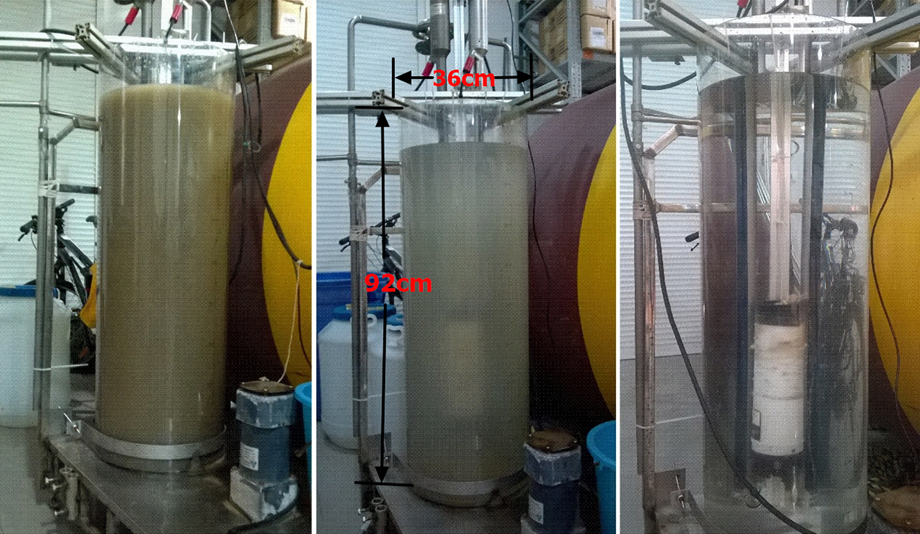
Experimental platform (left: high-concentration group, center: low-concentration group, right: clear water group).
The core component is a settling cylinder with a height of 92 cm and an inner diameter of 36 cm. The integrated system comprises the following key elements:
-
A movable platform chassis.
-
A high-range and a low-range Argus Suspension Meter (ASM) for comprehensive concentration measurement.
-
An optical backscatter sensor (OBS).
-
A fixed bottom agitator and a handheld auxiliary agitator.
-
A sliding sampling tube assembly.
Compared to traditional settling cylinders, this newly designed device offers several significant advantages:
-
High-Resolution, Non-Intrusive Profiling: Sensors are mounted at 1 cm intervals, recording data at 1-second intervals. This configuration enables continuous, high-resolution observation of the settling dynamics without disturbing the water column. Parameters such as sediment concentration, salinity, and temperature can be monitored in real time at specific depths.
-
Enhanced Measurement Capability and Portability: The dual-range ASM system ensures high accuracy across an extended measurement range. The integrated mobile chassis significantly improves the portability of the entire setup.
-
Complementary Spatial Sampling: The built-in sliding sampling tube allows for discrete water sample collection at various depths, providing data that validates and complements the continuous sensor measurements.
-
Guaranteed Homogeneity: The combination of a fixed bottom agitator and an auxiliary handheld agitator ensures the initial and sustained homogeneity of the sediment-water mixture throughout the experiment.
In summary, this innovative apparatus represents a substantial improvement over traditional static settling columns, enabling high-resolution, real-time investigation of sediment settling behavior under controlled conditions.
2.2 Sample collection and experiment preparation
To ensure that the experimental conditions closely resemble the natural conditions of the Yangtze Estuary, field campaigns were conducted to collect natural sediment, high-salinity seawater, and freshwater for the settling experiments. The sampling locations are shown in Figure 2.
Figure 2
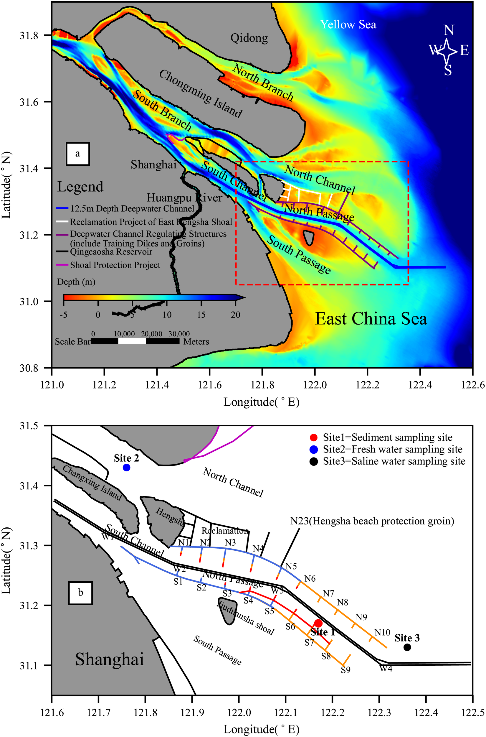
Location of three sampling sites in the Yangtze Estuary. (a) Bathymetry map of the Yangtze Estuary. (b) Locations of the sampling sites. Sediment samples were collected at site 1, located downstream of the North Passage. Freshwater samples were taken at site 2, in the middle of the North Channel, where freshwater dominates. Saline water was collected at site 3, where dominated by saline water.
Sediment samples were obtained from the mid-lower reach of the North Passage on May 14, 2015. Due to the large quantity of sediment required for the extensive test series, it was impractical to rely solely on suspended sediment collected directly from the water column, as repeated settlement and concentration would be prohibitively time-consuming. Therefore, an alternative preparation method was employed.
Bottom mud was collected from the seabed at the sampling site, alongside suspended sediment from the mid-depth (0.5H) of the water column. In the laboratory, the bottom mud was diluted with freshwater. After allowing coarser particles to settle, the supernatant rich in fine particles were repeatedly extracted. The grain size distribution of this processed sediment was then analyzed and confirmed to match that of the naturally collected suspended sediment from the mid-depth water column. This procedure ensured that the experimental sediment samples were representative of the in-situ suspended material while providing a sufficient volume for testing. The median particle size (D50) of the prepared samples was approximately 16 μm. The particle size distribution curves of the laboratory-prepared sediment samples and the natural mid-layer suspended sediment are closely aligned (Figure 3), with both having a median grain size of 16 μm. These results demonstrate that the sediment prepared for this experiment accurately represents the natural suspended sediment.
Figure 3
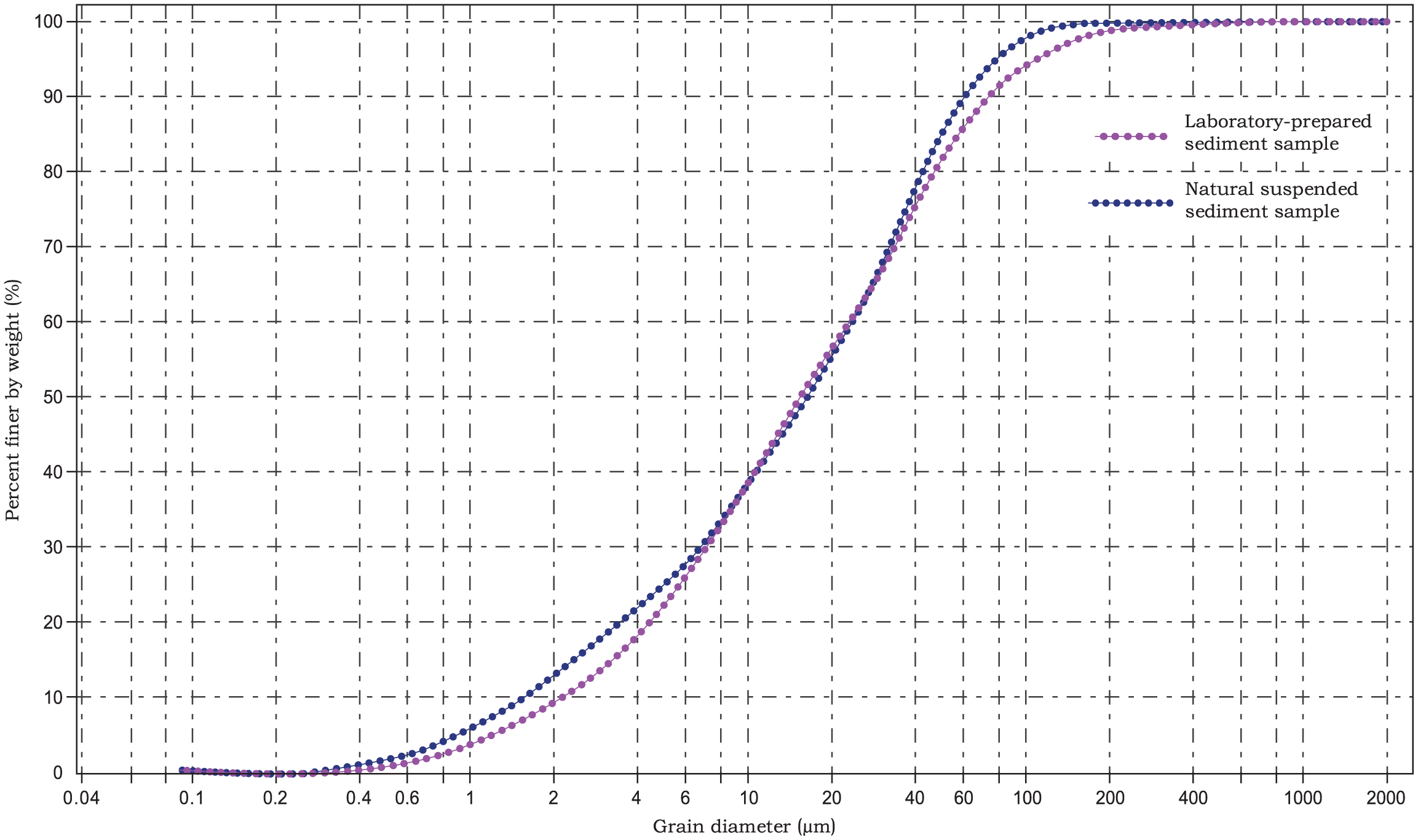
Comparison of the particle size distributions of the two sediment samples (The red line represents the natural suspended sediment sample; the blue line represents the laboratory-prepared sediment sample).
In previous studies on sediment settling experiments, various water types have been employed. Results indicate that the measured SV of sediment varies significantly depending on the water medium, with natural undisturbed water yielding more representative accurate results compared to purified or artificially prepared alternatives (Wan et al., 2015). To ensure quality of water samples for this study, natural freshwater and high-salinity seawater were collected separately from the middle reach of the North Channel and an offshore site southeast of the Deepwater Navigation Channel, respectively (Figure 2b).
2.3 Instrument configuration and calibration
The core measuring instrument in this experimental platform is the ASM sensor. The ASM sensor array consists of multiple individual sensors positioned at 1 cm intervals, providing a high vertical spatial resolution. It is capable of generating high-resolution SSC profiles at 1cm intervals when concentrations remain below saturation levels (typically SSC< 9 kg/m3) (Lin et al., 2020).
The optical measurement principle of the ASM presents a trade-off: accurate data at high concentrations require a sensor with a large measurement range, whereas higher precision at low concentration is achieved with a low-range sensor. To ensure precise measurements across the wide spectrum of SSCs encountered in this study, both high-range and low-range ASMs were integrated into the platform in a specific structural configuration. Extensive tests were conducted to confirm the absence of mutual interference between the co-located sensors.
This dual-range instrument configuration not only enhances measurement accuracy across different concentration regimes but also effectively extends the overall measurable SSC range. The integrated system thereby guarantees the acquisition of high-quality, continuous spatiotemporal data throughout the experiments.
Furthermore, extensive interference tests were conducted to ensure that no mutual interference occurred between the different sensors when operated simultaneously. The integration of both high- and low-range instruments enhances experimental accuracy and extends the overall measurement range, thereby ensuring the collection of high-quality, continuous spatiotemporal data throughout the experiments.
Prior to the formal experiments, all sensors (ASM and OBS) were calibrated using the prepared sediment samples. As illustrated in Figure 4, this calibration established the relationship between the optical signals (in Formazin Turbidity Units, FTU, or Nephelometric Turbidity Units, NTU) and the corresponding sediment concentrations. This step is essential for converting the instruments’ raw readings into accurate suspended sediment concentration (SSC) values, as it defines the correlation specific to the optical properties of the sediment used.
Figure 4
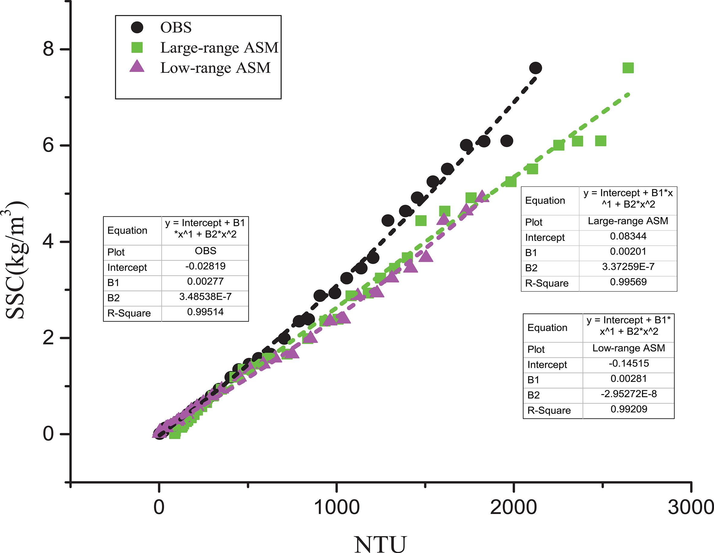
Calibration of Large-range ASM, Low-range ASM & OBS.
2.4 Experimental design
Based on the actual variations in salinity and SSC in the Yangtze Estuary, this study designed specific experimental groups to ensure a reasonable range of salinity and SSC values. The experiment was conducted under stable temperature conditions (23 ± 0.5°C) and a consistent water depth (approximately 90 ± 0.5 cm).
Salinity was set at 11 levels: 0, 0.5, 1, 2, 4, 6, 8, 12, 16, 23, and 30 PSU (Practical Salinity Unit). Sediment concentration was set at 19 levels: 0.15, 0.2, 0.3, 0.5, 0.7, 1, 1.2, 1.5, 1.7, 2, 2.2, 2.5, 2.7, 3, 4, 5, 6, 7, and 8 kg/m³ (Liu, 2025). A more intensive sampling of test conditions was implemented within sensitive ranges of these parameters, resulting in a total of over 200 individual settling tests.
2.5 Method to calculate SV
The SV was derived from the temporal evolution of SSC profiles by applying the principle of mass conservation. Under the assumption that the vertical diffusion term is negligible, the one-dimensional vertical mass balance equation reduces to the following form:
in which, c is the instantaneous sediment concentration at time t and depth h, t is the time, z is the height above the bed and ωs is the instantaneous, depth-dependent SV at depth h.
Integrating Equation 1 over depth, yields Equation 2:
An approximate solution by finite differences is Equation 3:
in which, represents the vertically averaged SV at time n, and are the vertically averaged sediment concentrations of at time n+1 and n, respectively, is the height of the water column after sample collection at time n and is the time interval between n+1 and n.
This McLaughlin formula provides instantaneous SV values at different water depths. However, during the actual settling process, the instantaneous SV varies at both temporally and spatially. To obtain a more representative value, this study adopts the median SV, defined as the average SV over the period t50–the time required for the initial sediment concentration to decrease by 50% at given depth (Pejrup and Mikkelsen, 2010; Portela et al., 2013; Wan et al., 2015). The median SV, as suggested by Burt (1986), is a common term used to described the settling velocity in laboratory experiment. The reason why median settling velocity is used instead of mean settling velocity is that fairly often only a little more than 50% of the settling velocity range can be described by use of the settling tube method because of the low settling velocity (Pejrup and Mikkelsen, 2010). The median settling velocity W50 was calculated according to the method described by the bottom withdrawal method (Sedimentation, 1953; Owen, 1976).
The median SV(ω50) was calculated by integrating the instantaneous, depth-dependent SV() overt the time interval t50 by Equation 4:
in which, t50 is the elapsed time after the SSC decreased to 50% of its initial value at a specific depth.
The McLaughlin formula is widely used in fine sediment studies (You, 2004; Wan et al., 2015) due to its solid physical basis, as it closely aligns with the fundamental definition of SV.
2.6 Experimental procedure
The experimental procedure consisted of the following sequential steps:
-
Salinity Configuration: The salinity was first adjusted according to the experimental plan. The original high-salinity water was diluted with fresh water collected from the Yangtze Estuary to achieve the target salinity. The water level in the settling cylinder was maintained at approximately 90 cm throughout this process. A bottom-mounted stirrer, assisted by auxiliary stirrers, ensured thorough mixing of the suspension. Salinity was monitored in real-time, and the water level was kept constant.
-
Sediment Concentration Configuration: The predetermined mass of prepared sediment was gradually injected into the cylinder while continuous stirring ensured its even distribution. This process was repeated until the target suspended sediment concentration (SSC) was reached. During this stage, water temperature and bottom-layer salinity were monitored in real-time, and the water level was kept constant.
-
Initiation of Settling Experiment: The stirring device was activated to homogenize the suspension completely. After stirring cease, the suspension was allowed to stand for 3 minutes to reach a near-static state. The experiment commenced at time t0, with vertical SSC profiles recorded at 1-mintue intervals. Data collection continued until the SSC in the representative near-bottom water layer decreases to 50% of its initial background value, recorded as time t50. This procedure generated continuous SSC profile data with a spatial resolution of 1 cm and a temporal resolution of 1 minute.
-
Settling Velocities Calculation. The instantaneous sediment SV was calculated from the continuous profile data using Equation 3. The median SV (ω50) for each layer was then determined using Equation 4. The median SV of the near-bottom water layer was adopted as the representative SV for the specific salinity and SSC condition.
3 Results and analysis
3.1 Representative settling process
Figure 5 presents the time series of SV across various water layers under four representative conditions: low salinity and low SSC, high salinity and low SSC, low salinity and high SSC, and high salinity and high SSC. A common trend observed under all representative conditions is that: the SV increases progressively from the upper layers to the lower layers. However, significant differences exist in the temporal evolution of SV among the different scenarios.
Figure 5
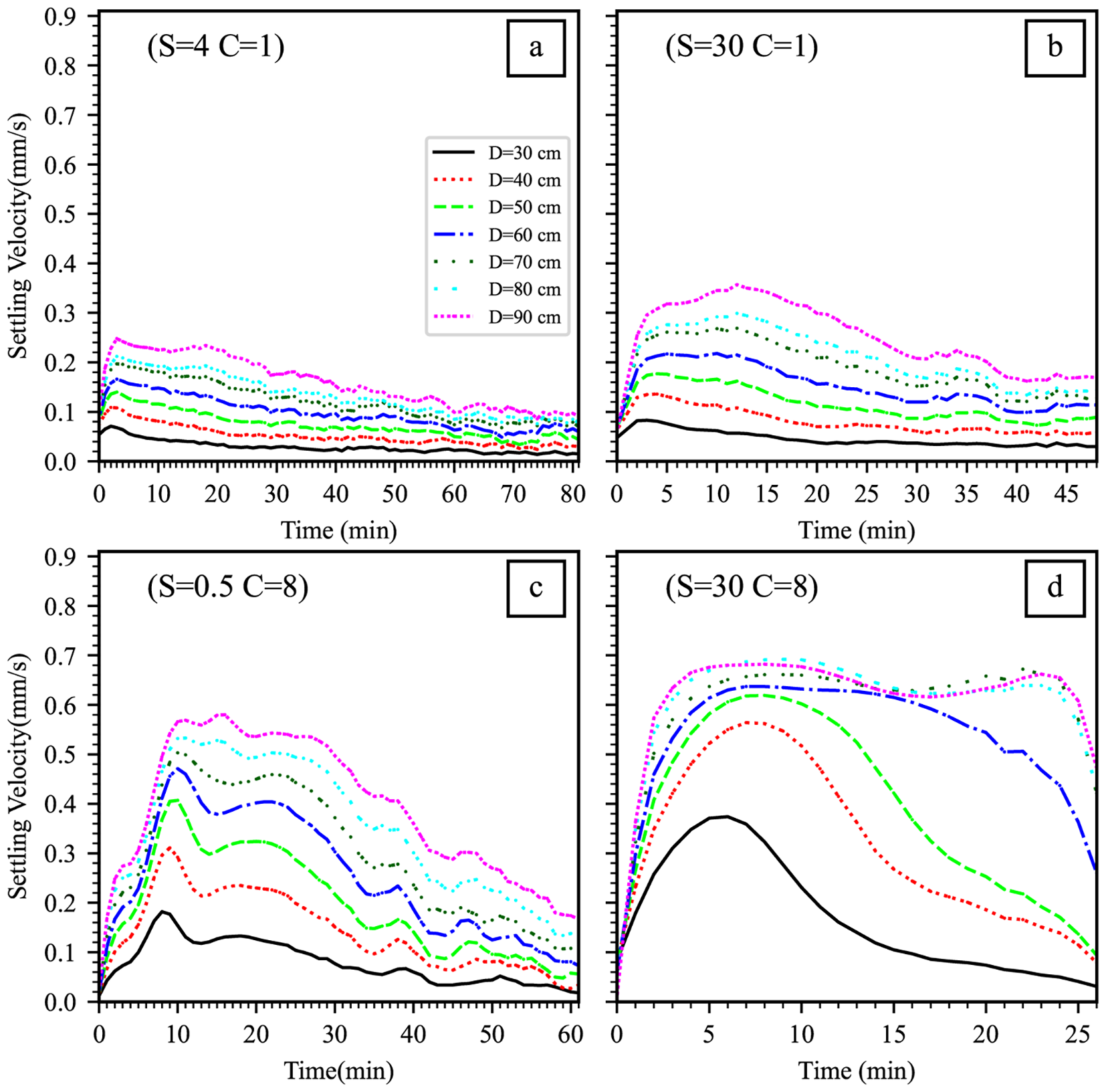
The time series of sediment SV under four representative conditions. (a) low salinity and low SSC (S = 4 PSU; C = 1 kg/m³), (b) high salinity and low SSC (S = 30 PSU; C = 1 kg/m³), (c) low salinity and high SSC (S = 0.5 PSU; C = 8 kg/m³) and (d) high salinity and high SSC (S = 30 PSU; C = 8 kg/m³). The color lines represent the time series of sediment SV variation at depths of different distance below the water surface.
a) Low Salinity and Low SSC (Figure 5a):
In this scenario, the settling process appears uniform across all water layers due to weak flocculation. The SV rapidly reaches a maximum (approximately 0.08–0.24 mm/s, depending on depth) within a few minutes and then decreases very gradually over the subsequent hour. The consistent settling rates across layers indicate minimal flocculation-induced stratification.
b) High Salinity and Low SSC (Figure 5b):
Here, flocculation plays a more significant role, particularly in the lower layers. In the surface layers, SV peaks (about 0.09–0.38 mm/s, depending on the depth) within minutes and declines slowly. In contrast, the center and bottom layers takes approximately ten minutes to reach peak SV, after which it gradually declines with minor fluctuations over the subsequent hour. The pronounced settling observed throughout the water column indicates that the increased salinity promotes the formation of larger flocs, thereby enhancing settling rates, especially in deeper layers.
c) Low Salinity and High SSC (Figure 5c):
Under these conditions, distinct SV peaks are evident in each layer (ranging from 0.18 to 0.6 mm/s). The ascending limb of each peak reflects the flocculation-accelerated settling phase, where particle aggregation enhances the settling rate. The descending limb represents the subsequent phase where coarser particles have deposited, leaving finer particles with lower settling velocities in suspension, thereby reducing the average SV over time. This pattern indicates more complex flocculation dynamics compared to low SSC conditions.
d)High Salinity and High SSC (Figure 5d):
In this scenario, sediment in the upper layers settles rapidly initially. The SV in these layers peaks (between 0.38 and 0.7 mm/s) within 5–7 minutes but then decreases drastically over the next twenty minutes. Meanwhile, SV in the lower layers remains nearly constant during this period. The settling process is significantly accelerated by high salinity, with the overall duration markedly shorter than under low salinity and low SSC conditions. The synergistic effect of high SSC, which increases particle collision frequency, and high salinity, which strengthens inter-particle bonding, leads to the rapid formation of large flocs and an accelerated settling process.
3.2 Distribution of settling velocity
The median SV of cohesive fine sediment from the Yangtze Estuary was determined using the methodology described in Section 2. The resulting SV distribution, presented as an isoline map in Figure 6a, clearly illustrates it variation across a spectrum of salinity and SSC conditions.
Figure 6
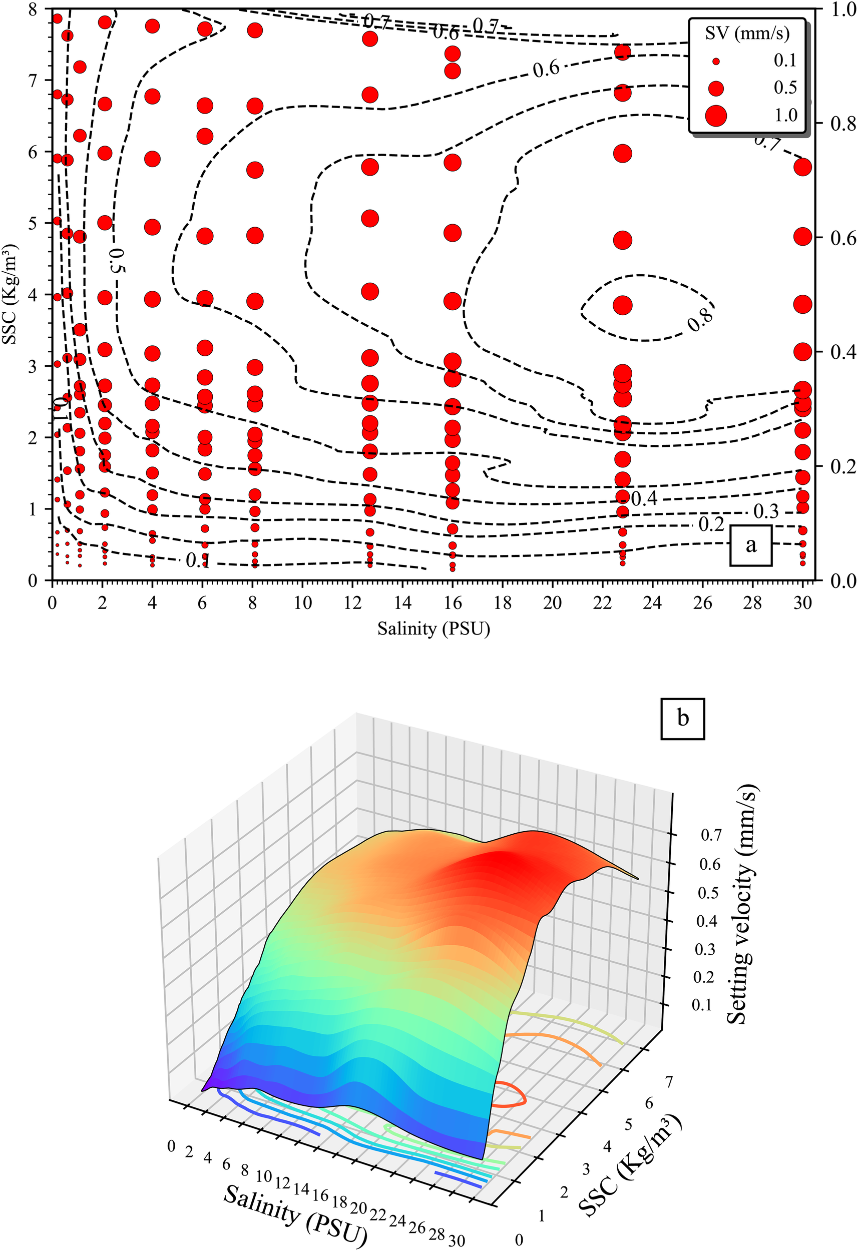
The distribution of sediment SV under various salinity and SSC conditions, revealing two distinct ridges (a) This plane distribution shows the experimental settings, where red circles represent different combinations of sediment concentrations and salinities. The diameter of each circle reflects the SV in that particular condition, with larger circle diameters indicating higher settling velocities. (b) The curved surface depicts the SV distribution in three dimensions, using cold colors (blue/green) to represent lower SV values and warm colors (orange/red) for higher values. This visualization allows a more intuitive understanding of how SV changes across the SSC-salinity space.
The isolines map reveals distinct regimes. In regions of low SSC (<1.5 kg/m³), the SV isolines are relatively straight and parallel across the entire salinity range (0–30 PSU). A similar pattern is observed under low salinity conditions (<0.5 PSU), where straight isolines extend across the full SSC range (0–8 kg/m³). These patterns indicate consistently low SV values, suggesting weak flocculation and slow settling rates where particle aggregation is minimal.
In contrast, a more complex isoline pattern emerges at high SSC (>1.5 kg/m³) and salinity levels (>0.5 PSU). The highest SV values appear within an SSC range of 3.5~4.5 kg/m³ and a salinity range of 21.5~26 PSU salinity, indicating a zone of intense flocculation activity. The absolute maximum SV of 0.9 mm/s was recorded at 4 kg/m³ SSC and 23 PSU salinity.
The three-dimensional representation of the SV distribution (Figure 6b) reinforces these trends. The surface exhibits an irregular, curve morphology. Low SV values, depicted in cool colors, dominate the region of low SSC and salinity, while the highest values, shown in warm colors, form a prominent ridge in the area of moderate SSC and salinity. This visualization further underscores that optimal conditions for flocculation and enhanced settling occur at moderate to high levels of both SSC and salinity.
Collectively, these findings highlight the synergistic influence of SSC and salinity on sediment settling behavior, with the most significant flocculation and highest settling velocities occurring within a specific, moderate range of these two factors.
The SV distribution is characterized by two prominent ridges, each representing a distinct pathway for flocculation enhancement:
a) The SSC-Driven Ridge: As SSC increases from 1 to 8 kg/m³, a ridge of maximum SV values emerges within a salinity range of 10–22 PSU. This pattern indicates that the elevated SSC can enhance particle collision probability. At high sediment concentrations, differential settling is a more significant mechanism in addition to Brownian motion, turbulent shear. Particles of varying sizes, shapes, and densities exhibit different settling velocities. Faster-settling larger particles effectively “overtake” and capture slower-settling smaller particles. As the sediment concentration increases, the number of particles per unit volume rises, causing the probability of these overtaking collisions to grow exponentially (Winterwerp, 1998, 2002). As the concentration is increased, the increased more frequency of inter-particle collision causes greater flocculation, resulting in large flocs of low density, Individually, these flocs can have a greater or lesser settling velocity depending on the relative changes in density and size, but usually a higher settling velocity. However, the increase in volume concentration of the results.
b) The Salinity-Driven Ridge: A second ridge, quite distinct from the hindered settling ridge induced by SSC, is observed as salinity increases from 1 to 22.8 PSU, with peak SV values occurring at moderated SSC levels of 2–7 kg/m³. The SV increases with rising salinity until reaching a peak value and then declines, which is consistent with previous studies (Mikeš and Manning, 2010; Abolfazli and Strom, 2023). The exact cause of declining settling velocities past the peak remains unclear. A potential explanation involves salinity’s flocculation effect reaching its maximum around 22–26 PSU. Once this threshold is passed, flocs tend to behave as if non-cohesive, or even undergo partial de-flocculation under high salinity conditions. As a result, any further rise in salinity reduces settling velocity through two mechanisms: increased specific gravity of the suspension and enhanced de-flocculation. This feature highlights the critical role of salinity in compressing the electrical double layer and enhancing electrochemical interactions between particles, which reduce repulsive forces, thereby fostering flocculation even without exceptionally high sediment concentrations (Ou et al., 2016).
These ridges reflect two different pathways for maximizing sediment settling: one driven by increasing SSC and the other by increasing salinity. Both factors significantly influence the aggregation and settling behavior of cohesive fine sediments.
3.3 Effect of sediment concentration
For cohesionless sediment, the effect of SSC is solely to reduce SV by increasing the volumetric concentration of the suspension. The associated increase in the volumetric concentration of the suspension tends to reduce the SV, as hindered settling is primarily a function of the volumetric concentration.
For cohesive sediment, the relationship between SSC and SV is more complicated. An increase in SSC leads to more frequent inter-particle collisions, which promotes flocculation and the formation of larger, low-density flocs, which increase the SV. The isolines of sediment SV at various salinities, illustrated in Figure 7, provide tangible evidence of the significant and complex influence of SSC and salinity on the SV of fine-grained sediment. The interaction is highly nonlinear, with different effects dominating at different concentration and salinity levels. ntu reanage the iment,anuscript At low SSC, the role of salinity in enhancing flocculation is more pronounced, leading to an increase in SV due to the formation of larger flocs. At high SSC, the effect of hindered settling becomes dominant, reducing the SV even though floc size may increase due to higher collision rates. These findings underscore the intricate relationship between salinity and SSC in determining the SV of cohesive sediments, with both factors contributing to a highly variable and context-dependent settling behavior.
Figure 7
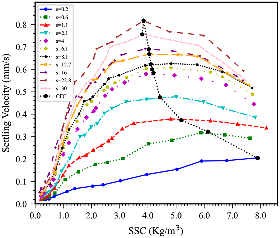
The sediment SV isohalines. The color curves are median SV isohaline under different salinity. The color dots are experimental data and black pentagon points are CFC value at different salinity.
The map includes eleven isolines representing SV across varying salinity levels. These isolines shown a consistent upward trend as salinity increases from 0.2 to 22.8 PSU. Within the SSC range of 0 to 4 kg/m³ SSC, rising SSC significantly enhances the probability of collisions among fine sediment particles, promoting aggregation and leading to an increase in SV.
This effect is most pronounced within the range of 0 to 2 kg/m3, beyond which the rate of SV increase gradually slows as SSC rises from 2 to 4 kg/m3. When SSC exceeds a certain threshold, SV begins to decrease, making the transition into the hindered settling phase. Thus, the overall settling process encompasses both an accelerated flocculated-dominated phase and a decelerated hindered settling phase.
More specifically, within the 0 to 2 kg/m3 range, SV increases notably due to enhanced flocculation and the formation of larger flocs. However, as SSC surpasses 2 kg/m3, the rate of SV increase diminishes, and once SSC exceeds a critical value—typically around 4 kg/m3—SV starts to decline. This decline signifies the onset of hindered settling, where increased particle crowding inhibits the downward motion of flocs.
The settling process of cohesive sediment thus consists of two distinct phases: a) Accelerated flocculated settling, during which flocculation dominates, increasing the SV. b) Decelerated hindered settling, where higher particle concentrations result in crowding, thus reducing the SV due to hindered settling.
This dual-phase behavior has been reported in the literature (Mehta et al., 1989; Winterwerp, 2002; Mikkelsen et al., 2007; Manning et al., 2010; Wan et al., 2015). The present findings further underscore the complex nature of fine sediment settling under varying salinity and SSC conditions.
At low salinity levels (0.2 and 0.6 PSU), the sediment SV increases gradually with rising SSC, showing a relatively small gradient. Between 6 to 8 kg/m³, the SV stabilizes with minimal variation. In contrast, under higher salinity levels conditions (above 0.6 PSU), the SV increases more rapidly as SSC rises, exhibiting a considerably steeper gradient.
At a salinity of 0.6 PSU, the SV reaches a maximum value of 0.47 mm/s at an SSC of 6.7 kg/m3. Beyond this point, as SSC increases to 7.62 kg/m3, the SV begins to decrease. This turning point indicates the onset of hindered settling, where excessive SSC leads to the formation of a particle network that restricts sedimentation, significantly reducing SV.
A similar pattern is observed at 1.1 PSU salinity, where the maximum SV of 0.498 mm/s occurs at 6.22 kg/m3 SSC. This trend continues at salinity levels above 1.1 PSU, with a clear decrease in SV beyond a critical SSC value. This critical value, which marks the transition to hindered settling, is defined as the critical flocculation concentration (CFC).
At lower salinities (0.2, 0.6, and 1.1 PSU), the CFC remains around 7 kg/m3. In contrast, as salinity increases above 2.1 PSU, the CFC decreases to approximately 4 kg/m3. This result demonstrates that the CFC is highly sensitive to salinity, decreasing as salinity increases—a pattern consistent with observations from mud settling tests in the Severn Estuary.
3.4 Effect of salinity
Fine clay particles are negatively charged on their surface and are surrounded by a cloud of cations. This cloud comprises two layers: the Stern layer, which is immediately adjacent to the particle surface with a high cation concentration, and the outer Gouy layer, where the ion concentration gradually decreases. Together, these layers form the diffusive double layer. The double layer is characterized by the ζ-potential (ζ0) at the water-particle interface, which decreases proportionally with increasing ion concentration. The thickness of this double layer depends on the mineral type, ion concentration in the medium, and the balance between attractive electrical forces and diffusion (Van Leussen, 1994).
The interaction between two approaching particles is governed by the overlap of their double layer. Repulsive electrical forces tend to separate the particles, but if these forces are overcome at a certain distance, collisions can occur, allowing particles to adhere via attractive forces. The energy of this electrical barrier varies significantly with ion concentration. In natural waters, dissolved salts release free ions and cations, which reduce the energy barrier; at moderate to high salt concentrations, this barrier can be eliminated entirely (Maggi, 2005). The ζ-potential—and thus the cohesion—of minerals like kaolinite is influenced by salt concentration (Vane and Zang, 1997).
For cohesionless sediment, the primary effect of salinity is to increase the specific gravity of suspension, thereby slightly reducing the SV. However, the effect is more complicated for cohesive fine sediment. The salinity usually has two opposite effects on cohesive fine sediment. On one hand, an increase in salinity raises the specific gravity of suspension, which tends to slightly reduce the SV. On the other hand, within a certain range, increasing salinity enhances flocculation. Higher salinity weakens repulsive forces, leading to an increased rate of particle collisions and floc formation, ultimately resulting in a higher SV.
The median SV is plotted against salinity at various SSC in the semi-logarithmic coordinate system (Figure 8). At salinity level below 16 PSU, the effect of enhanced flocculation significantly outweighs the effect of the increased sediment suspension specific gravity. This leads to a rapid increase in SV with rising salinity, reflected by a steep gradient. However, this gradient diminishes at SSCs of 6.81 and 7.67 kg/m³, corresponding to the hindered settling phase. In this phase, the influence of salinity on SV is reduced, as the high SSC induces a settling process dominated by hindered settling mechanisms.
Figure 8
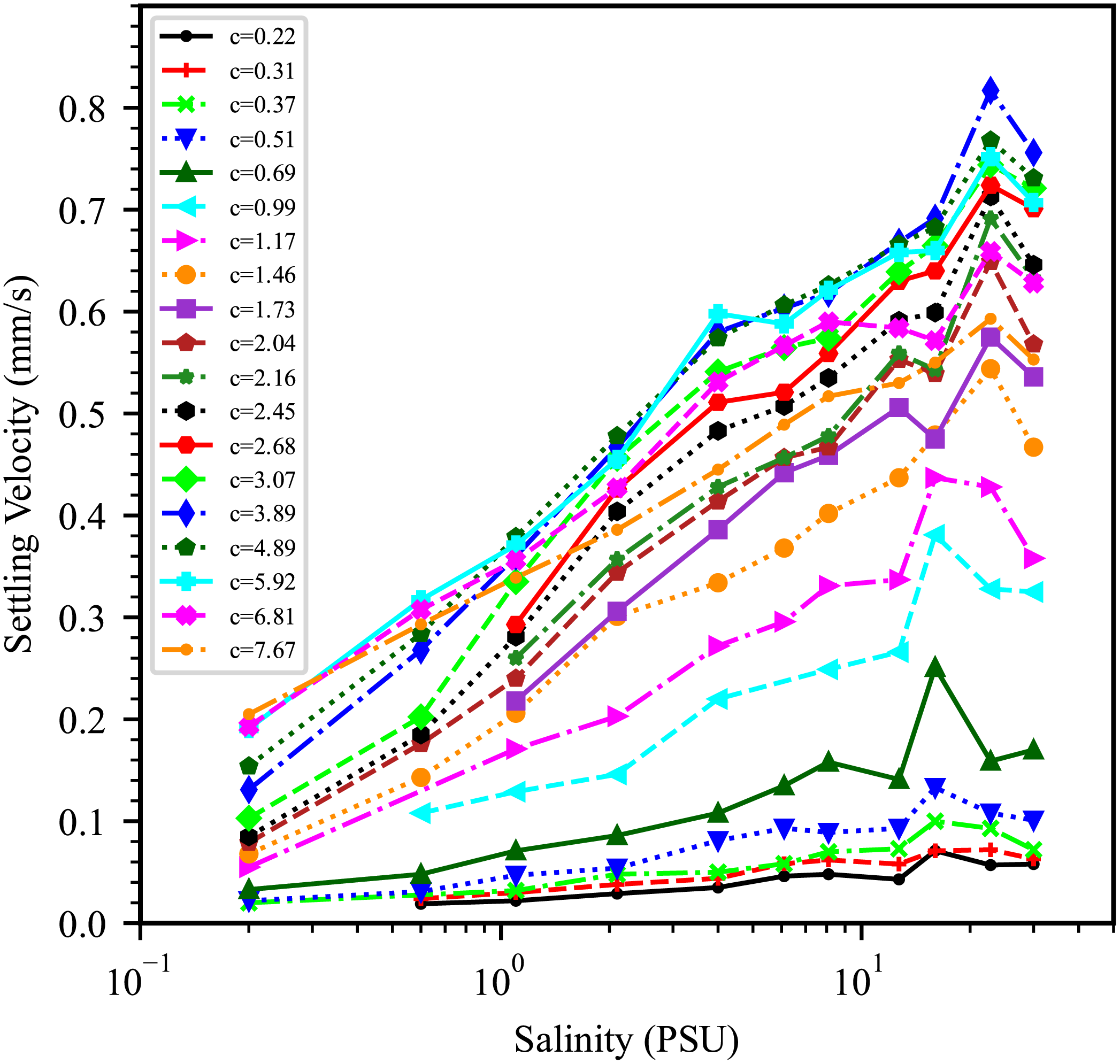
The sediment SV against salinity in the semilog coordinate system. The color curves are median SV varying with salinity at various SSC.
For each SSC level, the SV initially increases with rising salinity until reaching a peak value, after which it declines. At SSCs greater than 1.17 kg/m³, the SV at 22.8 PSU salinity is higher than that at both 16 PSU and 30 PSU. Conversely, at SSCs below 1.17 kg/m³, the SV at 16 PSU is higher than that at 12.7 PSU and 22.8 PSU. Therefore, the critical flocculation salinity (CFS) for maximum flocculation lies within the range of 16 to 22.8 PSU, depending on SSC. Prior to the onset of hindered settling, the CFS appears to increase proportionally with SSC, although high-resolution data would be needed to confirm the trend conclusively.
Previous research stated that the CFS for sediment in the Yangtze Estuary is about 7 PSU during dry seasons and 10 PSU in wet seasons (Wan et al., 2015), which is considerably lower than the CFS values (16 to 22.8 PSU) observed in this experiment. Several factors such as experimental methods, water chemistry, and sediment properties could also contribute to this discrepancy. The median particle size (D50) of the prepared samples is 8 μm in Wan et al. (2015) but 16 μm in this experiment.
Beyond the CFS, further increases in salinity reduce the SV due to the combined effects of increased suspension specific gravity and the onset of de-flocculation. Thus, the CFS represents the salinity threshold at which the sediment settling transitions from a flocculation acceleration phase into a retarded settling phase.
3.5 Effect of temperature
Temperature influences the behavior of individual particles and the motion of flocs, thereby affecting the SV. Although direct tests on temperature were not conducted in this experiment, a review of its effect on sediment SV can provides useful insights.
Within the framework of the Derjaguin–Landau–Verwey–Overbeek (DLVO) theory (Lyklema et al., 1999; Pierre and Ma, 1999; Missana and Adell, 2000), the interaction forces between particles are considered the sum of van der Waals attractive forces and electrical double-layer repulsive forces. The flocculation ability of clay particles is governed by the balance between these forces. When the inter-particle distance is less than 25 nm, the two forces–the double-layer forces (an electrostatic force arising from the overlap of electrical double layer) and the van der Waals forces(an inherent molecular attraction)– become dominant (Lau, 1994; Qiao et al., 2019). While the van der Waals attractive force remains nearly constant for a given particle size and separation distance, the electrical double-layer repulsive force is highly sensitive to environmental factors such as temperature, pH, ionic strength of the liquid medium, and the surface charge density of the particles (Flatt, 2004; Wallevik, 2005; Jurado and Espinosa-Marzal, 2017; Huang et al., 2022).These factors collectively determine the flocculation potential by modulating the repulsive or attractive interactions between particles.
Higher temperatures can reduce the stability of the electrical double layer, weakening the repulsive force and thereby enhancing flocculation, which in turn increases the SV. Conversely, lower temperatures may reinforce the repulsive forces, reducing flocculation and consequently decreasing the SV.
The mean floc size and floc volume tend to increase with rising temperature. At low temperatures, floc formation is hindered due to reduced frequencies of particle collision and capture. While higher temperatures generally promote the floc formation, the resulting flocs can become unstable and prone to breakage. This occurs because the hydrodynamic forces (e.g., turbulence and fluid shear) acting on flocs become comparable in magnitude to the short-range inter-particle binding forces. This phenomenon has been numerically simulated for interactions between primary particles (Qiao et al., 2017).
Several studies report that SV increases with rising temperature at a given sediment concentration. In fact, when temperature exceeds 25°C, the rate of SV increase significantly more pronounced (Jing et al., 2024). Experiments have also demonstrated that elevated temperatures positively influence floc SV, with a more substantial effect observed at higher SSCs. However, this temperature effect diminishes once the settling process enters the hindered settling phase (Wan et al., 2015). Nevertheless, over the normal environmental range, the influence of temperature on SV is minor compared to the effects of concentration, salinity, or settling depth (Owen, 1972).
Temperature primarily affects SV mainly through its change on water viscosity, in accordance with Stokes Law (Equation 5), which states that SV is proportional to v-l, v is the kinematic viscosity (Equation 6). Therefore, it is standard practice to correct for temperature effects by assuming SV is inversely proportional to the kinematic viscosity. Consequently, an increase in temperature reduces water viscosity and, according to Stokes’ Law, accelerates the SV.
In this equation, is the primary particle diameter(m), is kinematic viscosity(mm2/s), which is a function of temperature, and T is water temperature (0C).
4 Discussion
4.1 Conceptual analogy model
The Langmuir isotherm model, developed by Irving Langmuir in 1916, describes the dependence of the surface coverage of an adsorbed gas on the pressure of the gas above the surface at a fixed temperature (Langmuir, 1918). It explains adsorption process by assuming that adsorbate behaves as an ideal gas at isothermal conditions (Hanaor et al., 2014) and adsorption and desorption are reversible processes. It can also describe the effect of pressure and temperature on adsorption process during the interaction between gas phase and solid surface (Roger, 2024).
This paper proposes a bold hypothesis that the flocculation process of fine sediment particles influenced by salinity and temperature is highly analogous to the process of gas molecule adsorption on solid surfaces described by the Langmuir isotherm model. To address these complexities, this paper proposes a particle aggregate conceptual analogy model to describe sediment particle aggregation. A schematic of particle or floc aggregation in the flocculation process is illustrated in Figure 9. This model adapts Langmuir’s principles to the more intricate nature of sediment particle interactions, accounting for environmental variables that influence floc formation and SV.
Figure 9
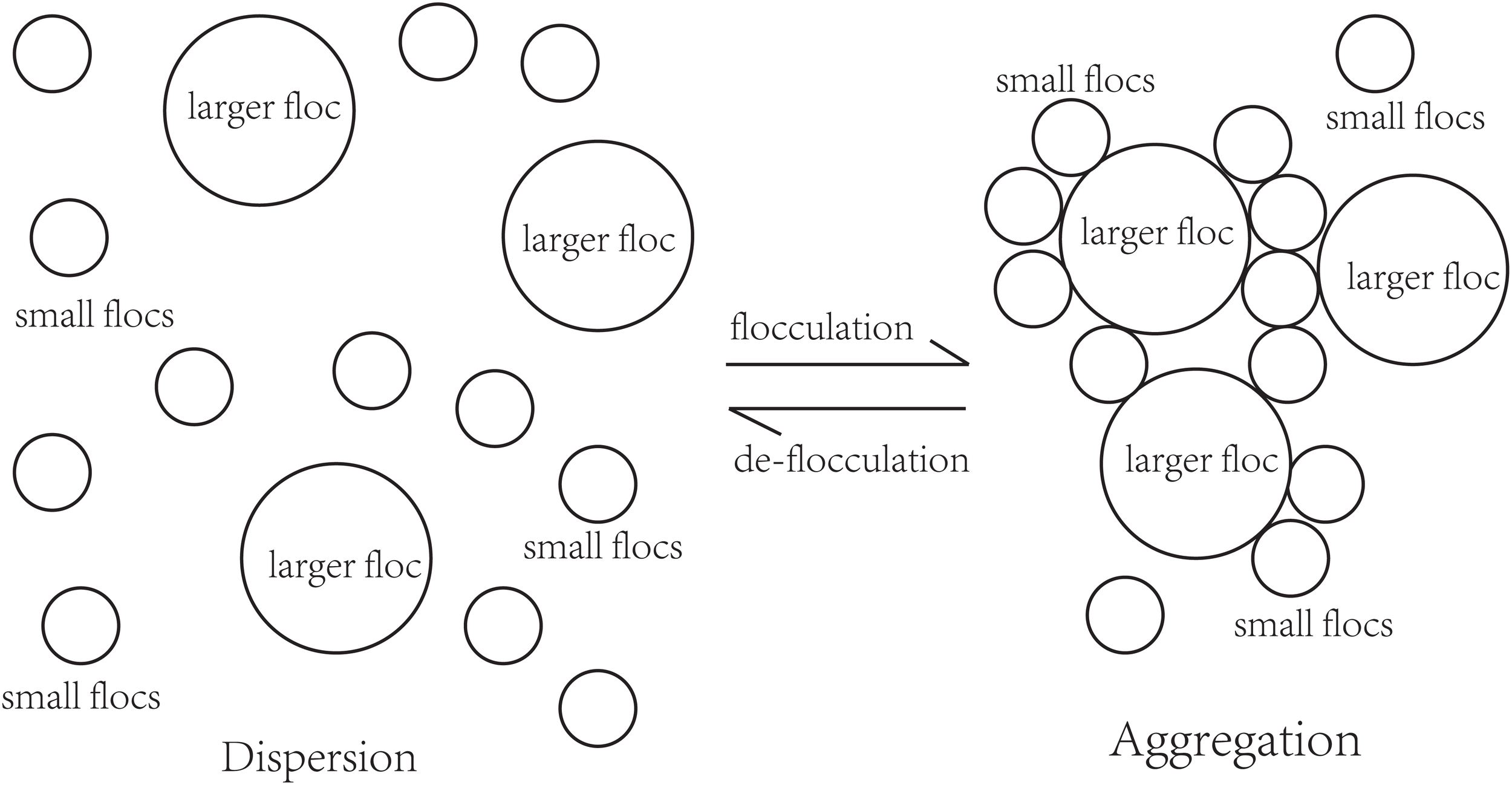
The schematic of sediment particle or floc aggregation.
This conceptual analogy model conceptualizes the sediment particle aggregation process by treating it as analogous to gas adsorption, where small particles or flocs form a continuous monolayer surrounding the surface of a larger particle or floc. In this conceptual analogy model, the aggregation is treated as an equilibrium process during adsorption and desorption. The equilibrium is established between the small particle phase (), the vacant surface sites of the larger particle or floc, and the particles adsorbed onto the surface. For a non-dissociative aggregation process, this can be expressed as Equation 7:
Where:
- represents the primary particles or small flocs in suspension, - represents a large particle or developed floc with abundant vacant surface sites, - represents a larger floc after aggregation, which could act as adsorbent to adsorb more particles.
This equilibrium equation expresses the reversible interaction between small particles and available surface sites of large flocs. The rates of aggregation (flocculation) and disaggregation (de-flocculation) are assumed to balance at equilibrium, allowing the derivation of further equations for predicting the aggregation behavior under varying conditions, such as salinity and sediment concentration.
To describe the reversible processes of aggregation and dispersion, as described in Equation 8, we define an equilibrium constant K, in terms of the concentrations of “reactants” and “products”, which characterizes the balance between the rate of particle aggregation onto the surface of large flocs and the rate of dispersion, where larger flocs break back into smaller flocs or particles. The equilibrium is reached when these two rates are equal. We can express the equilibrium constant K in terms of these quantities. The equilibrium expression is given by:
We may also note that:
- is proportional to the surface coverage of large particles or flocs, denoted as θ (the fraction of the surface that is occupied by smaller particles or flocs), - [S] is proportional to the number of vacant sites, denoted as (1-θ) (the fraction of the surface that remains unoccupied), - [] is proportional to the salinity, S, reflecting the concentration of small particles affected by salinity.
Hence, it is also possible to define another equilibrium constant, k (is proportional to but not exactly equivalent to K), as given below:
Where:
- represents the surface coverage of the larger particles or flocs by smaller ones,
- S represents the salinity, which influences the aggregation process.
This equilibrium expression reflects how the aggregation process depends on both the salinity S and the available surface coverage . As salinity increases, the aggregation process becomes more favorable, leading to a higher surface coverage of large particles or flocs. However, the equilibrium also accounts for the reversibility of the process, where dispersion counterbalances aggregation under certain conditions.
By rearranging Equation 9, we can solve for (the degree of surface coverage) as a function of salinity:
This equation shows how surface coverage parameter increases with salinity S, reaching saturation as S becomes large.
Equation 10 is the primary mathematical formulation of expressing the conceptual analogy model. As with all chemical reactions, the equilibrium constant, , is both salinity-dependent and related to the Van der Waals attraction and double layer electrostatic repulsion forces, according to DLVO theory, and hence related to the enthalpy change for the aggregation process.
Note two extremes in Equations 11, 12:
At low salinity:
At high salinity:
At a given SSC and salinity condition, the extent of particle aggregation is determined by the value of k, which is dependent upon both the temperature (T) and the enthalpy (heat) of adsorption. The magnitude of the aggregate enthalpy reflects the strength of binding of a particle to a floc. Increasing temperature has a positive effect on SV (Wan et al., 2015), which means flocculation is enhanced and fractional surface coverage increase as temperature rising.
The characteristic aggregates variation of coverage with effect of salinity for particle aggregation is illustrated in the Figure 10. Under a specific SSC and salinity condition, the extent of particle aggregation is determined by the value of k, which depends on temperature (T) and the enthalpy of adsorption. The enthalpy reflects the binding strength of a particle to a floc and higher enthalpy indicates stronger binding. As temperature increases, the SV also tends to rise (Wan et al., 2015), suggesting increased fractional surface coverage and enhanced flocculation. This relationship illustrates how temperature can facilitate aggregation by altering the dynamics of particle interactions.
Figure 10

The coverage isohaline varies with different values of k, which is influenced by temperature T as well as the interactions between sediment concentration and salinity.
Figure 10 visually represents the variation in aggregate coverage in various salinity, highlighting the impact of salinity on the aggregation process. Higher salinity can lead to increased floc formation and coverage, enhancing the overall aggregation effect under specific temperature conditions.
The coverage isohalines provide valuable insights into how these factors influence floc formation and stability under varying conditions. As the value of k changes, it alters the rate of aggregation and, consequently, the surface coverage of particles on larger flocs. Higher values of k typically indicate stronger interactions, leading to greater aggregation and increased coverage. Conversely, lower values may result in reduced aggregation and lower surface coverage.
The k value increases with higher system temperatures and the interactions between temperature, sediment concentration, and salinity. Thus, the curves depicted in Figure 9 illustrate the effects of either (i) increasing the magnitude of the adsorption enthalpy at a fixed temperature or (ii) elevating water temperature along with the interplay between temperature, sediment concentration, and salinity. This relationship highlights the complex interactions among these factors in shaping aggregation dynamics in sedimentary environments.
4.2 Formula with concentration and salinity
When river water carrying fine colloidal particles mixes with electrolyte-rich seawater, the resulting sediment deposition often leads to the formation of sandbars and deltas at the river mouth. Numerical modeling is a crucial tool for studying these sediment transport and deposition processes in estuaries, and the SV is a key parameter in such models. Therefore, a practical and unified formula for SV, incorporating primary particle diameter, SSC, salinity, and temperature, is essential for effective numerical simulations.
Inasmuch as collisions depend on particle concentration in the suspension, SSC can be used as an approximate lumped parameter for estimating the settling velocity of flocs. As a result, and given the convenience with which concentration can be easily measured, most formulas were setup relating the SV to SSC (Mehta and McAnally, 2008).
Following Wolanski et al. (1989), the overall settling process can be divided into four distinct zones: free settling, flocculation settling, hindered settling, and negligible settling. Hwang (1989) developed a formula encompassing both flocculation settling and hindered settling zones. The SV, , in each zone can be expressed as Equation 13:
Where, =free settling velocity; = suspension concentration; = scaling coefficient; = flocculation settling exponent; = hindered settling exponent; = hindered settling coefficient; = zone concentration limits defined in Figure 11.
Figure 11
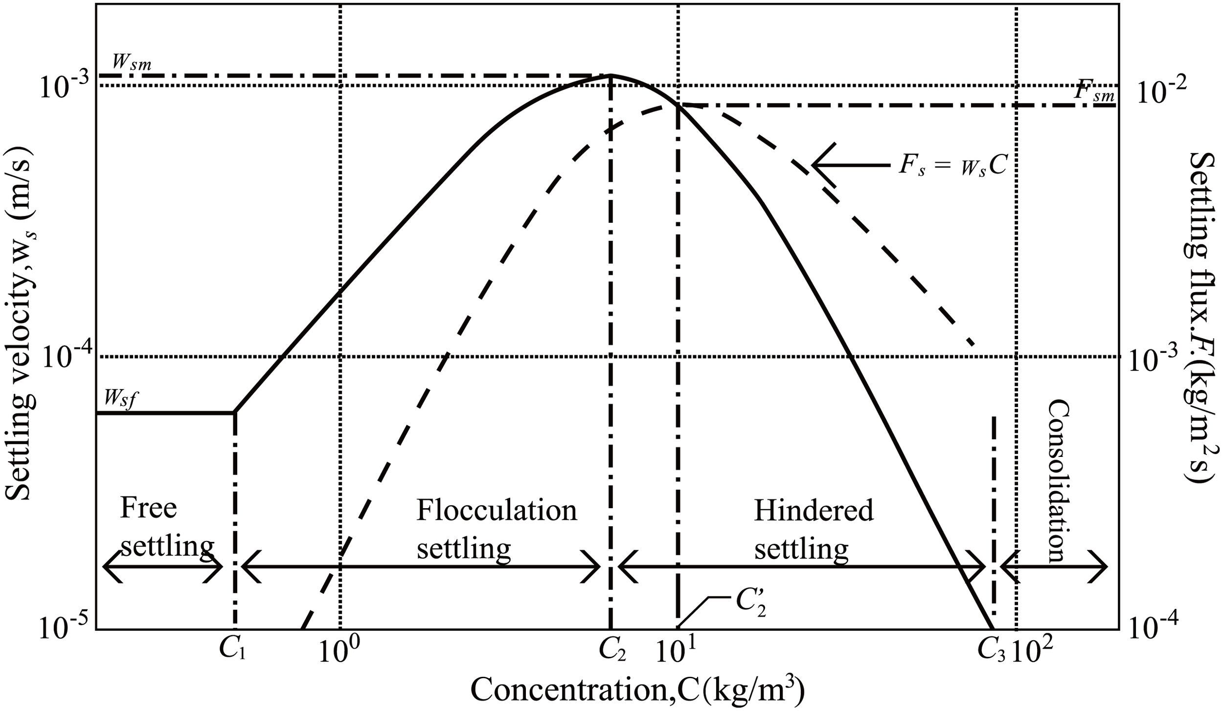
A representative plot of settling velocity and associated settling flux variation with suspension concentration (from Mehta and McAnally, 2008).
The is independent of C, and can be calculated from Stokes’ law during free settling at low suspension concentration. The increases with increasing SSC due to flocculation between and , which is in flocculation settling zone. The value is 0.2 kg/m3 in this experiment. The is critical concentration related to peak SV(). The decreases with increasing C in the hindered settling zone between and . At concentration above , settling becomes comparatively small as consolidation takes over.
It can be observed from Figure 7 that within the relatively low salinity range (e.g., 0.2 to d 8.1 PSU), the SV increases sharply with increasing salinity. The influence of salinity on SV is particularly significant within this range. In contrast, within the higher salinity range (e.g., 8.1 to 32 PSU), the SV increases only slightly. Consequently, the influence of salinity on SV gradually diminishes as salinity rises. This saturation behavior closely resembles the characteristic shape of the Langmuir isotherm, which describes the adsorption process of gas molecules onto solid surfaces (Hanaor et al., 2014). Therefore, the classic Langmuir isotherm model can be adopted to characterize this feature.
The surface coverage parameter coefficient, , could be introduced to quantify the effect of salinity on flocculation process. At a given salinity the extent of flocculation is determined by the value of k. The effect of sediment concentration on flocculation can be modulated by interaction between salinity and sediment concentration.
A formula could be derived through the following procedure. First, the sets of independent parameter (a,b,m,n) are fitted for each discrete salinity value(s). Next, the variation patterns of the parameters (a,b,m,n) with salinity are analyzed, and their functional relationships (e.g., linear, exponential, power-law) are established. As demonstrated in Figure 12, The selection process of fitting function was based on a comparison of goodness-of-fit metrics (R² and RMSE) among linear, exponential and power functions. The power function consistently yielded the highest R2 value for b,m,n. For parameter a, although the linear function achieved the highest R2 (0.6068), followed by power function (0.5706), but the difference is small. Therefore, the power function was chosen as fitted function for parameters (a,b,m,n) for consistency.
Figure 12
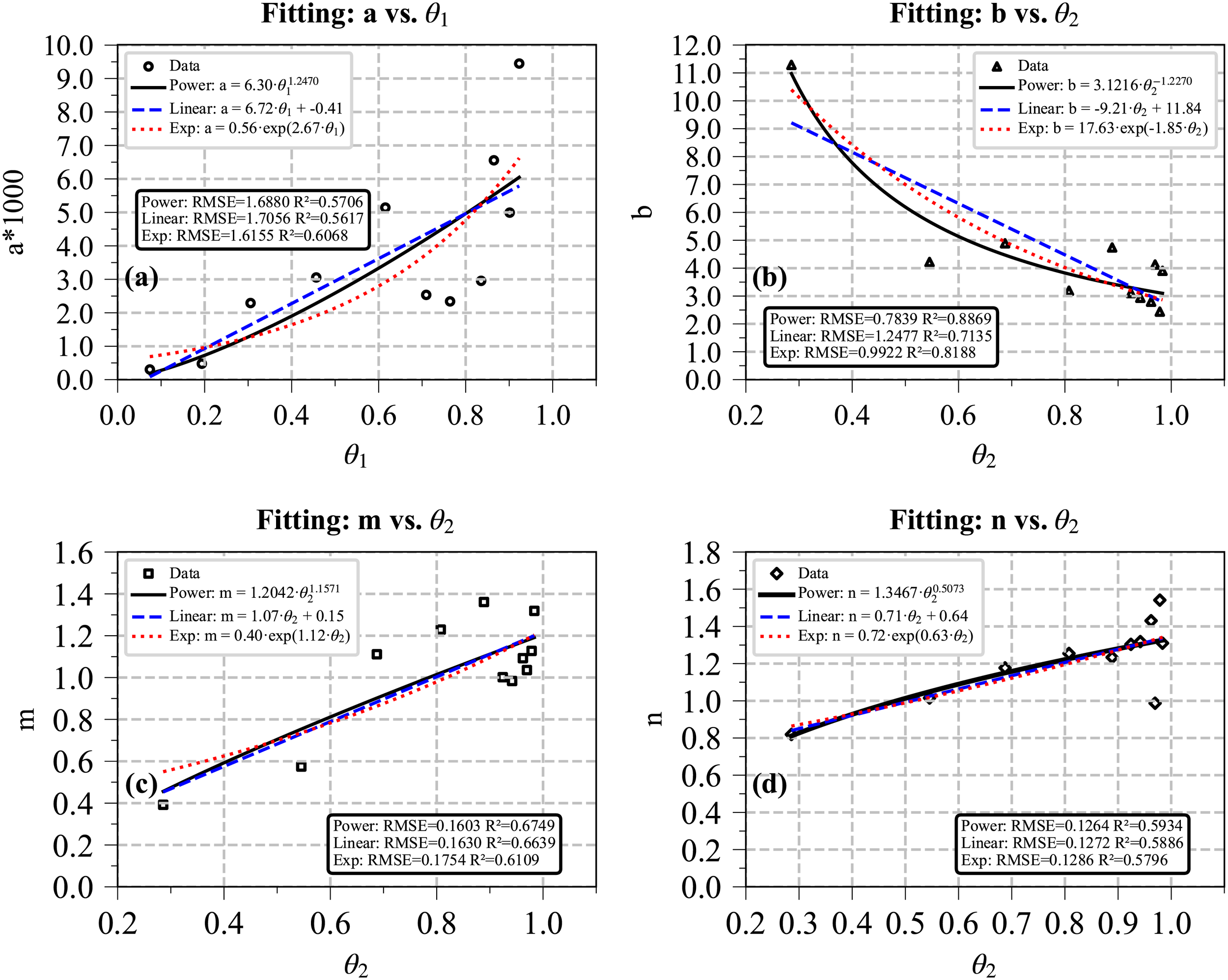
Comparison of fitting relationship among linear, exponential, and power functions between the parameters a, b, m,n and , which increase with increasing salinity.
Finally, a comprehensive formula across a continuous range of salinity values is obtained:
Where, a(s), b(s), m(s), and n(s) are functions of salinity as Equations 15–18. The terms , and are coefficients, while , and are exponents of power functions. The parameters and in Equation 19 represent the direct effect of salinity and the interactive effect between salinity and sediment concentration on flocculation, respectively. As illustrated in Figure 12, the parameters a, b, m and n can be expressed power functions of or . The corresponding coefficients and exponent for these functions are listed in Table 1.
Table 1
| Parameters | a | b | m | n | |
|---|---|---|---|---|---|
| Coefficient | 0.0063 | 3.1216 | 1.2042 | 1.3467 | |
| Exponent | 1.2470 | -1.2270 | 1.1571 | 0.5073 | |
The coefficients and exponent of power functions.
To determine the appropriate values for parameters k1 and k2, multiple sets of k1 and k2 are used to calculate the corresponding R² values for Equation 14 along with parameters (a,b,m,n) and the results are compared. As shown in the Figure 13a, when k2 was set to 2, 3, or 4, the R² of Equation 14 reaches its maximum when k1 is between 0.4 and 0.6. Therefore, a value of k1 = 0.5 is considered appropriate. Furthermore, with k1 fixed at 0.4, 0.5, or 0.6, Equation 14 maintained high R² values across k2 range of 1.5~4 (Figure 13b), while parameters b, m, and n also exhibited high R2 values in this interval (Figure 13d). Thus, the combination k1 = 0.5 and k2 = 3 is determined to be optimal.
Figure 13
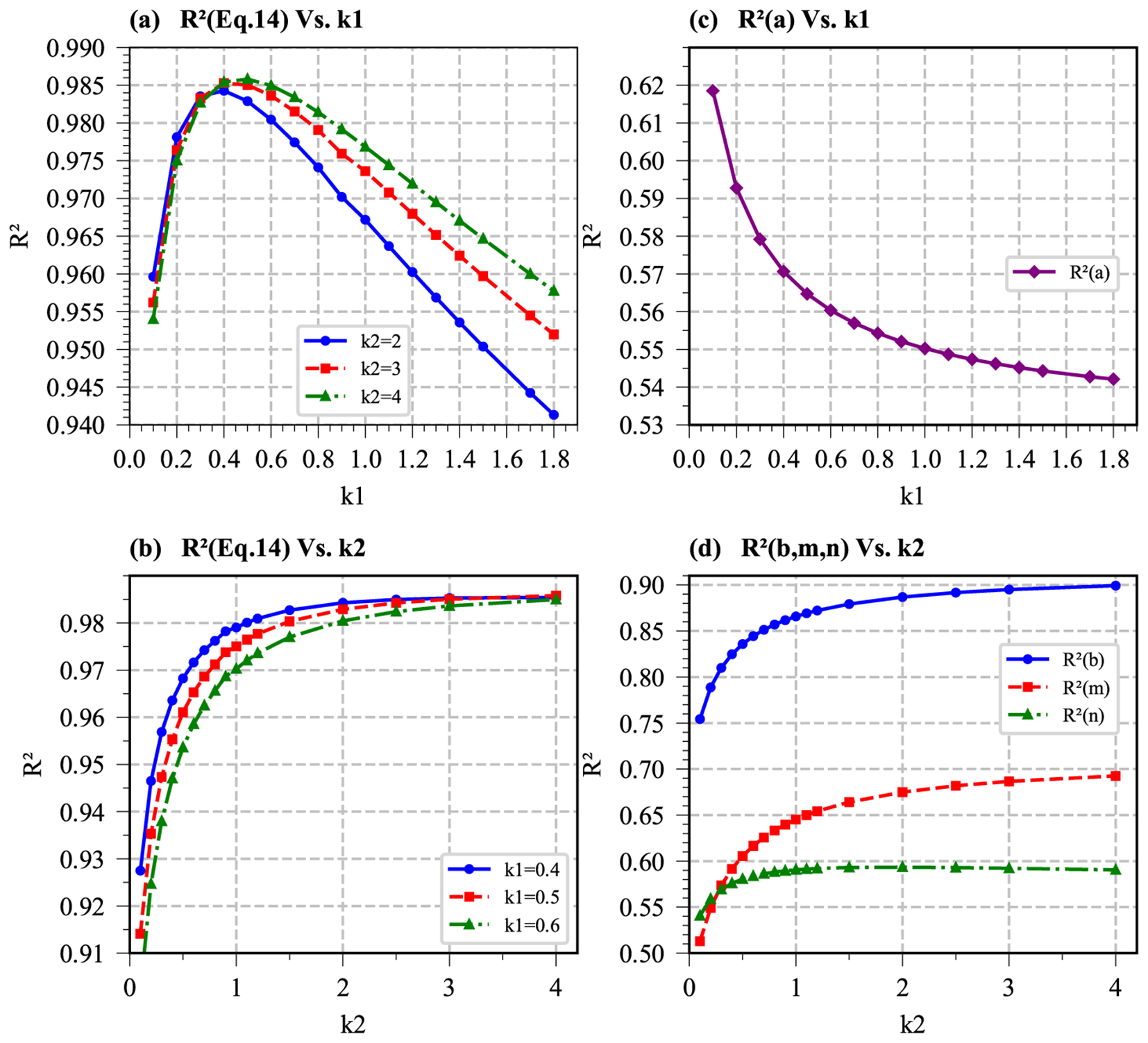
The R2 value for Equation 14 and a,b,m,n at various parameters k1,k2.
This proposed formula incorporates the effects of both SSC and salinity, enabling predictions of SV across both the flocculation-accelerated and hindered settling phases under varying SSC and salinity conditions. A comparison between formula predicted SV and experimental data is presented in Figure 14, which demonstrates excellent agreement and effectively captures the influence of key factors on SV. The following two skill assessments are commonly employed to evaluate the proposed formula performance: coefficient of determination (R²) and root mean square error (RMSE). The result shows R2 = 0.9850 and RMSE = 0.0355mm/s, which demonstrate that the proposed formula, with its four fitted parameters, is capable of predicting settling velocity with a relatively small error.
Figure 14
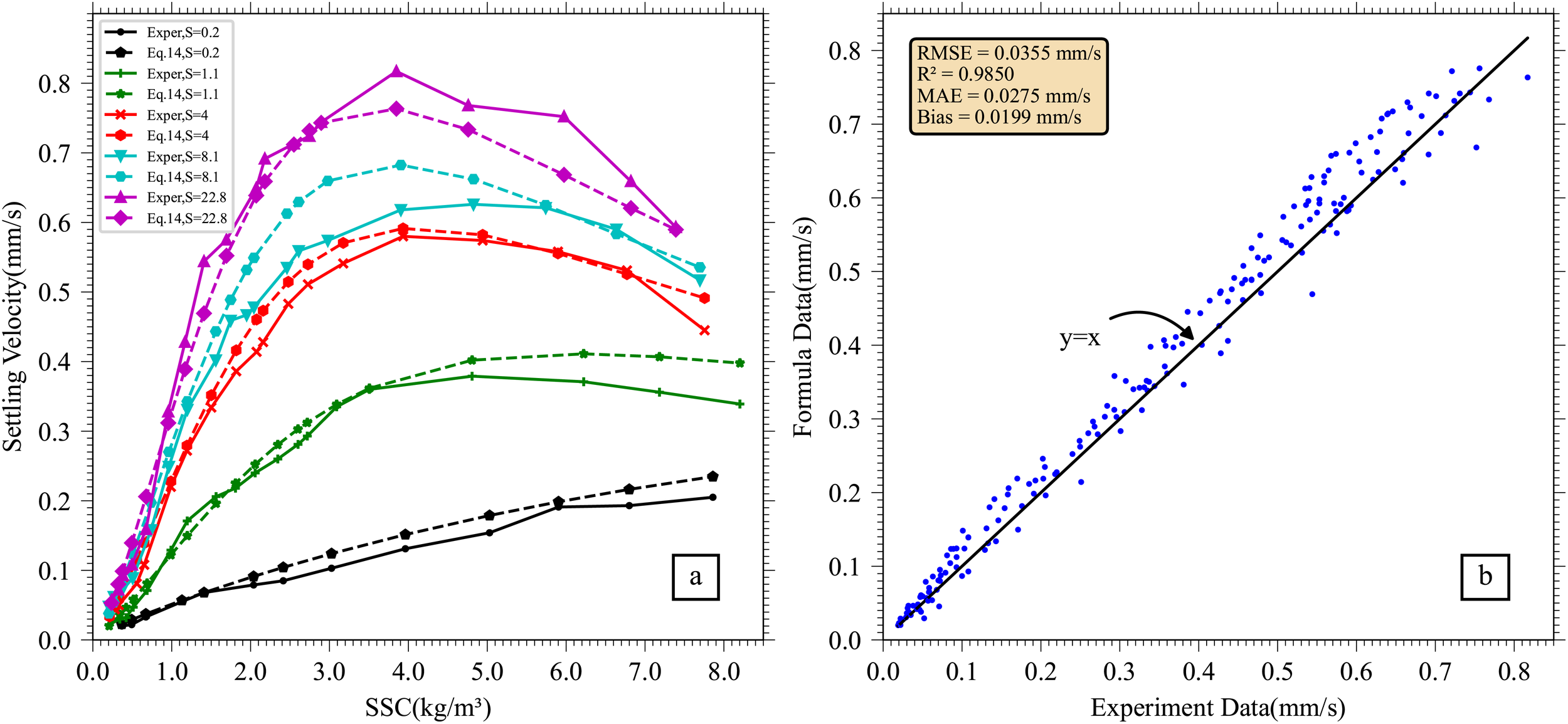
Comparison between the formula and experimental data. (a) The isohaline curves derived from the formula are compared with experimental data, demonstrating that the formula effectively describes the impact of SSC and salinity on SV, Exper. represent experiment data and Eq. 14 means formula data. (b) A comparison of all SV data obtained from the formula against experimental results. Dots above the line indicate formula-derived values greater than experimental values, while dots below the line indicate formula values that are lower. Dots on the line represent instances where formula data matches experimental data exactly.
4.3 Sensitivity analysis
Global sensitivity analysis was performed using the Sobol’ variance-based method (Sobol′, 2001) as implemented by Saltelli et al. (2010). This approach has been successfully applied in similar environmental modeling (Nossent et al., 2011), morphodynamic models (Van Der Wegen and Jaffe, 2013), and provides robust quantification of both individual parameter effects and parameter interactions.
A global sensitivity analysis was conducted using the Sobol’ method to quantify the influence of the input parameters on the model’s prediction of settling velocity. This variance-based technique decomposes the total output variance into contributions attributable to each parameter individually (first-order indices) and in combination with others (total-order indices), thereby effectively identifying key drivers and parameter interactions. The global sensitivity analysis results are shown as Figure 15.
Figure 15

The global sensitivity analysis result, (a) First-order indices of all parameters, contributions attributable to each parameter individually, (b) Total-order indices of all parameters, contributions in combination with others. (c) Parameter importance ranking.
The results clearly demonstrate sediment concentration(C) is the most influential parameter, with the highest total-order sensitivity index (ST=0.471). This is followed by the model coefficient p3 (ST=0.297), which governs the exponent in the denominator of the formula. Salinity(s) also exhibits a moderate, yet significant, influence (ST=0.193). Furthermore, the notable difference between the total-order and first-order indices for both sediment concentration and parameter p3 indicates the presence of substantial nonlinear interactions with other parameters in the model. These findings underscore the primary roles of sediment concentration and the structural parameter p3 in controlling flocculation dynamics within this estuarine system.
4.4 Comparison with existing formulas
A performance comparison between the newly proposed formula and existing settling velocity formulas that account for the effects of salinity and concentration is warranted. Owen (1970) formula, calibrated by Mehta and McAnally (2008) from experiment dataset by Owen (1970), can predict SV under varying SSC and salinity, though it does not employ the same parameters as the proposed formula. Costa and Mehta (1991); Jiang (1999) formula, derived from experiment dataset by Mehta and McAnally (2008), and Hwang (1989) formula can predict SV under different SSC conditions but do not incorporate salinity effects. Therefore, Owen (1970); Costa and Mehta (1991); Jiang (1999) formula and Hwang (1989) formula are selected for comparison with Equation 14. As shown in Figure 16, the curves predicted by Equation 14 exhibit similar trends to those generated by the other formulas. Moreover, the SV values predicted by Equation 14 are closest to those obtained using the Costa and Mehta (1991) formula. The difference between formulas is due to different techniques of experiment, water chemistry, and to the differences in the sediment tested.
Figure 16
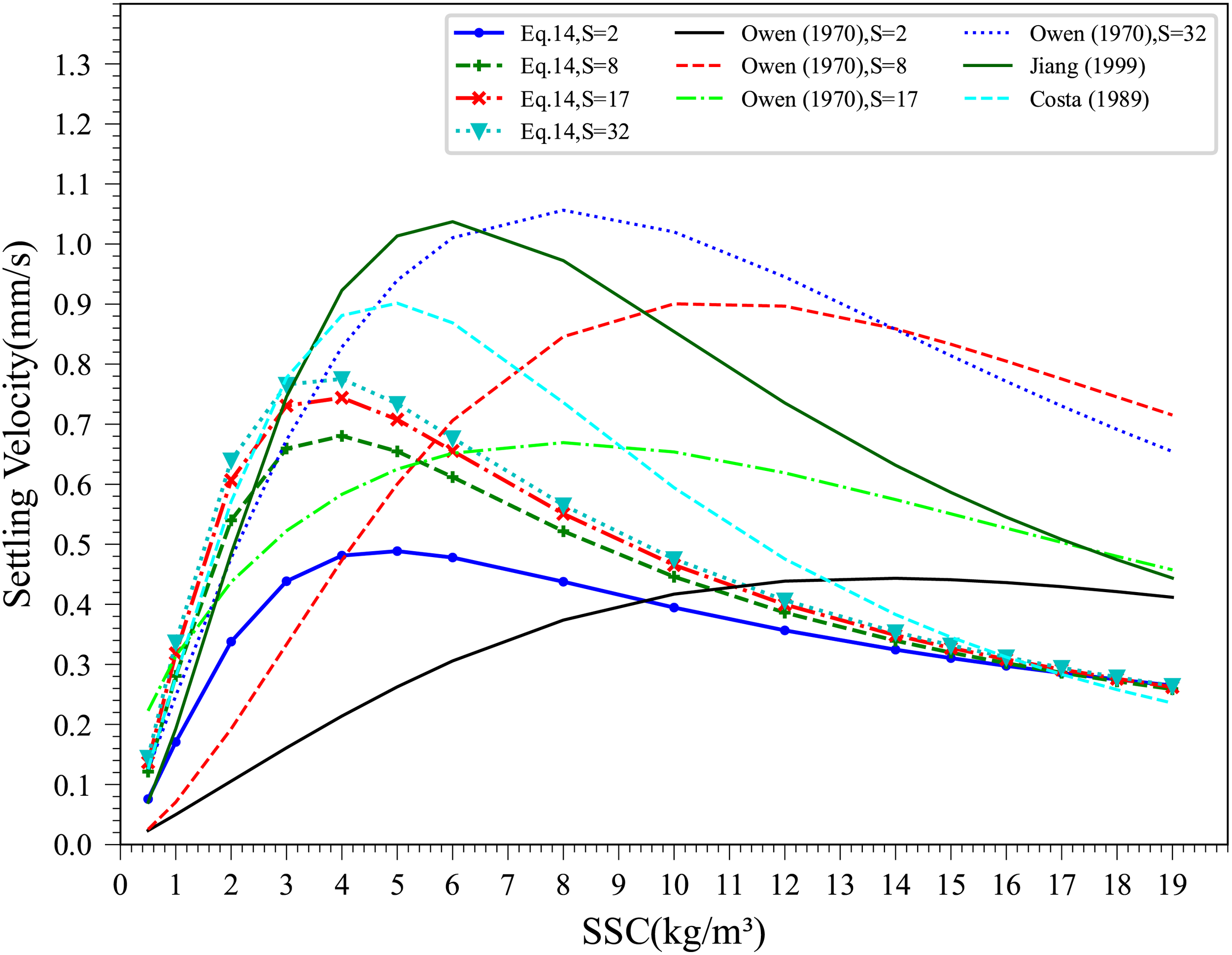
The performance comparison between the proposed formula and existing settling velocity formulas.
4.5 The peak SV and corresponding concentration
Some useful quantities related to SV, such as peak SV() and its corresponding concentration () – which is equivalent to the CFC discussed in Section 3.3 – can be derived from Equation 14.
The (Equation 20) and (Equation 21) are determined by salinity, as the coefficients of a, b, m and n are functions of salinity. Here, represents the theoretical equivalent of the CFC estimated from experiment data.
The variations of the peak velocity and corresponding concentration with salinity are shown in Figure 17. The peak velocity increases with salinity, rising at a faster rate when salinity is below 10 PSU and increasing at slower rated when salinity beyond 10 PSU. In contrast, the concentration decreases as salinity increases. This decrease is extremely rapid at salinities below 5 PSU, slows down considerably above 5 PSU, and gradually approaches a constant value at higher salinities. The CFC values estimated from experimental data show good agreement with those values predicted by the theoretical equation (Figure 17).
Figure 17
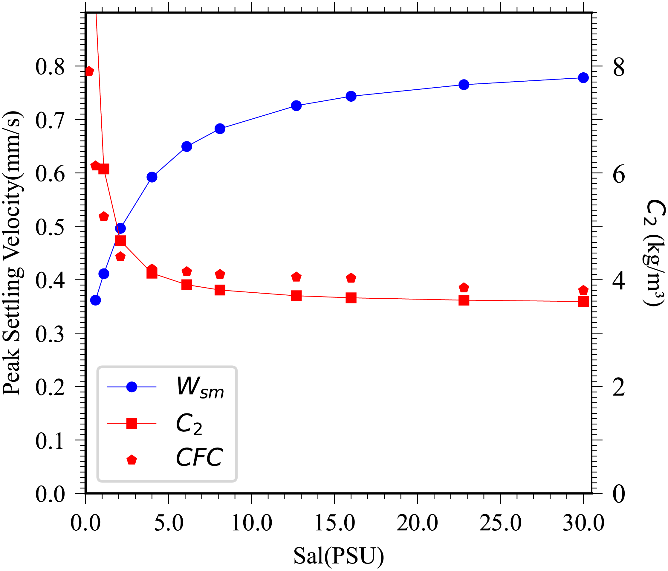
The peak velocity and corresponding concentration vary with salinity. The blue line with circle dot indicates the peak velocity , and the red line with square dot indicates corresponding concentration . The red pentagon points indicate the CFC values at various salinity.
4.6 Limitations and transferability of the empirical formula
The model parameters were calibrated to and are likely optimal for the specific hydrological, sedimentological, and chemical conditions of the studied estuary during the observation period. Consequently, the derived formula serves as an empirically constrained, process-informed parameterization for flocculation dynamics. It represents a case-specific empirical relationship that provides context-specific insights and a potential methodological framework, rather than a universally validated predictive model. Application to other estuaries would require recalibration of parameters (a, b, m, n) using local observational or experimental data. Its primary value lies in proposing a functional form and elucidating the interaction of key drivers (e.g., SSC, salinity) within flocculation-settling velocity system, which can inform the structuring of modules in broader settling velocity research.
5 Conclusions
This study provides a comprehensive experimental analysis of the SV of fine-grained sediment under varying salinity and sediment concentration conditions. The main conclusions are drawn as follows:
-
The interaction between SSC and salinity on SV is highly complex and nonlinear. High SSC promotes particle collisions, while increased salinity enhances flocculation, collectively accelerating the settling process. This interaction is manifested in the SV distribution as two distinct ridges: one formed by increasing SSC and the other by increasing salinity.
-
The critical flocculation concentration (CFC), marking the transition from flocculation-accelerated to hindered settling, is sensitive to salinity. The CFC decreases from approximately 7 kg/m³ under low salinity conditions to about 4 kg/m³ in high salinities. The critical flocculation salinity (CFS) for maximum flocculation ranges from 16 to 22.8 PSU, depending on SSC.
-
The median SV increases with SSC until reaching a peak value (occurring between 4 to 8 kg/m³, depending on salinity), beyond which hindered settling dominates and SV decreases.
-
A particle aggregate conceptual analogy model is proposed, along with a mathematical formulation to express this model. A new formula for predicting SV is proposed, incorporating sediment concentration and salinity as key factors. These parameters (a,b,m,n) within the formula are expressed as power function of surface coverage parameter , which is related to salinity. Predicted from the formula exhibit a close agreement with the experimental data, effectively capturing the SV behavior across both flocculation-accelerated and hindered settling phases.
-
The peak SV () increases with salinity, while the CFC decreases. Both trends can be accurately calculated from the theoretical equations derived in this study.
Statements
Data availability statement
The datasets presented in this study can be found in online repositories. The names of the repository/repositories and accession number(s) can be found below: https://doi.org/10.17632/pr78hn7nzy.1 Experiment data of sediment settling velocity.
Author contributions
GL: Investigation, Visualization, Conceptualization, Writing – review & editing, Writing – original draft, Methodology. YW: Resources, Software, Data curation, Writing – original draft, Validation, Methodology. JZ: Funding acquisition, Writing – review & editing, Project administration, Supervision.
Funding
The author(s) declared that financial support was received for this work and/or its publication. This research is found by National Key Research and Development Program of China (2023YFC3208500, 2022YFA1004404) and Key Project of the National Natural Science Foundation of China (U2340225).
Conflict of interest
Author YW was employed by the company Shanghai Investigation, Design & Research Institute Co., Ltd.
The remaining author(s) declared that this work was conducted in the absence of any commercial or financial relationships that could be construed as a potential conflict of interest.
Generative AI statement
The author(s) declared that generative AI was not used in the creation of this manuscript.
Any alternative text (alt text) provided alongside figures in this article has been generated by Frontiers with the support of artificial intelligence and reasonable efforts have been made to ensure accuracy, including review by the authors wherever possible. If you identify any issues, please contact us.
Publisher’s note
All claims expressed in this article are solely those of the authors and do not necessarily represent those of their affiliated organizations, or those of the publisher, the editors and the reviewers. Any product that may be evaluated in this article, or claim that may be made by its manufacturer, is not guaranteed or endorsed by the publisher.
References
1
Abolfazli E. Strom K. (2023). Salinity impacts on floc size and growth rate with and without natural organic matter. J. Geophys. Res. Oceans128, e2022JC019255. doi: 10.1029/2022JC019255
2
Agrawal Y. C. Pottsmith H. C. (2000). Instruments for particle size and settling velocity observations in sediment transport. Mar. Geol.168, 89–114. doi: 10.1016/S0025-3227(00)00044-X
3
Burt T. N. (1986). “ Field settling velocities of estuary muds,” in Lecture Notes on Coastal and Estuarine Studies. Ed. MehtaA. J. ( New York Inc.: Springer-Verlag), 126–150. doi: 10.1029/LN014p0126
4
Chen Q. Meng Y. Zhou J. Ding P. (2005). A review on flocculation of fine suspended sediments and its controlling factors in the Yangtze River estuary. Ocean Eng.23, 74–82. doi: 10.16483/j.issn.1005-9865.2005.01.012
5
Cole P. Miles G. V. (1983). Two-dimensional model of mud transport. J. Hydraul. Eng.109, 1–12. doi: 10.1061/(ASCE)0733-9429(1983)109:1(1
6
Costa R. G. Mehta A. J. (1991). “ Flow-fine sediment hysteresis in sediment-stratified coastal waters,” in Coastal Engineering 1990 ( American Society of Civil Engineers, Delft, The Netherlands), 2047–2060. doi: 10.1061/9780872627765.157
7
Flatt R. J. (2004). Dispersion forces in cement suspensions. Cem. Concr. Res.34, 399–408. doi: 10.1016/j.cemconres.2003.08.019
8
Gao J. Hou L. Liu Y. Shi H. (2024). Influences of bragg reflection on harbor resonance triggered by irregular wave groups. Ocean Eng.305, 117941. doi: 10.1016/j.oceaneng.2024.117941
9
Gao J. Ma X. Dong G. Chen H. Liu Q. Zang J. (2021). Investigation on the effects of Bragg reflection on harbor oscillations. Coast. Eng.170, 103977. doi: 10.1016/j.coastaleng.2021.103977
10
Guang X. Cheng Y. Du X. (1996). Experimental study on the flocculation mechanism in the Yangtze estuary. J. Hydraul. Eng.70–74. doi: 10.13243/j.cnki.slxb.1996.06.011
11
Guo L. He Q. (2011). Freshwater flocculation of suspended sediments in the Yangtze River, China. Ocean Dyn.61, 371–386. doi: 10.1007/s10236-011-0391-x
12
Guo C. He Q. Guo L. Winterwerp J. C. (2017). A study of in-situ sediment flocculation in the turbidity maxima of the Yangtze Estuary. Estuar. Coast. Shelf Sci.191, 1–9. doi: 10.1016/j.ecss.2017.04.001
13
Ha H. K. Maa J. P.-Y. (2010). Effects of suspended sediment concentration and turbulence on settling velocity of cohesive sediment. Geosci. J.14, 163–171. doi: 10.1007/s12303-010-0016-2
14
Hanaor D. A. H. Ghadiri M. Chrzanowski W. Gan Y. (2014). Scalable surface area characterization by electrokinetic analysis of complex anion adsorption. Langmuir30, 15143–15152. doi: 10.1021/la503581e
15
Huang T. Yuan Q. Zuo S. Yao H. Zhang K. Wang Y. et al . (2022). Physio-chemical effects on the temperature-dependent elasticity of cement paste during setting. Cem. Concr. Compos.134, 104769. doi: 10.1016/j.cemconcomp.2022.104769
16
Hwang K.-N. (1989). Erodibility of fine sediment in wave-dominated environments (florida, USA: University of Florida).
17
Jiang J. (1999). An examination of estuarine lutocline dynamics (Gainesville, Fla: University of Florida). doi: 10.5962/bhl.title.112388
18
Jing Y. Zhang J. Zhang Q. Maa J. (2024). Experimental study on the effects of sediment size gradation and suspended sediment concentration on the settling velocity, w. Powder Technol.437, 119541. doi: 10.1016/j.powtec.2024.119541
19
Jurado L. A. Espinosa-Marzal R. M. (2017). Insight into the electrical double layer of an ionic liquid on graphene. Sci. Rep.7, 4225. doi: 10.1038/s41598-017-04576-x
20
Langmuir I. (1918). The adsorption of gases on plane surfaces of glass, mica and platinum. J. Am. Chem. Soc40, 1361–1403. doi: 10.1021/ja02242a004
21
Lau Y. L. (1994). Temperature effect on settling velocity and deposition of cohesive sediments. J. Hydraul. Res.32, 41–51. doi: 10.1080/00221689409498788
22
Lick W. Huang H. Jepsen R. (1993). Flocculation of fine-grained sediments due to differential settling. J. Geophys. Res. Oceans98, 10279–10288. doi: 10.1029/93JC00519
23
Lin J. He Q. Guo L. van Prooijen B. C. Wang Z. B. (2020). An integrated optic and acoustic (IOA) approach for measuring suspended sediment concentration in highly turbid environments. Mar. Geol.421, 106062. doi: 10.1016/j.margeo.2019.106062
24
Liu G. (2025). “ Experiment data of sediment settling velocity”, Mendeley Data, V1. doi: 10.17632/pr78hn7nzy.1
25
Liu Q. Liu X. Chen J. Hou P. He Y. Wang Q. et al . (2023). Experimental study on flocculation and sedimentation characteristics of cohesive fine sediment measured using ultrasound in the Pearl River Estuary. Int. J. Sediment Res.38, 880–890. doi: 10.1016/j.ijsrc.2023.09.001
26
Lyklema J. Van Leeuwen H. P. Minor M. (1999). DLVO-theory, a dynamic re-interpretation. Adv. Colloid Interface Sci.83, 33–69. doi: 10.1016/S0001-8686(99)00011-1
27
Maa J. P.-Y. Kwon J.-I. (2007). Using ADV for cohesive sediment settling velocity measurements. Estuar. Coast. Shelf Sci.73, 351–354. doi: 10.1016/j.ecss.2007.01.008
28
Maggi F. (2005). Flocculation dynamics of cohesive sediment (Delft, Netherlands: Delft University of Technology).
29
Manning A. J. Dyer K. R. (1999). A laboratory examination of floc characteristics with regard to turbulent shearing. Mar. Geol.160, 147–170. doi: 10.1016/S0025-3227(99)00013-4
30
Manning A. J. Langston W. J. Jonas P. J. C. (2010). A review of sediment dynamics in the Severn Estuary: Influence of flocculation. Mar. pollut. Bull.61, 37–51. doi: 10.1016/j.marpolbul.2009.12.012
31
Mehta A. J. Hayter E. J. Parker W. R. Krone R. B. Teeter A. M. (1989). Cohesive sediment transport. I: process description. J. Hydraul. Eng.115, 1076–1093. doi: 10.1061/(ASCE)0733-9429(1989)115:8(1076
32
Mehta A. J. McAnally W. H. (Eds.) (2008). “ Fine-grained sediment transport,” in Sedimentation Engineering: Processes, Measurements, Modeling, and Practice ( American Society of Civil Engineers, Reston, VA). doi: 10.1061/9780784408148
33
Mikeš D. (2011). A simple floc-growth function for natural flocs in estuaries. Math. Geosci.43, 593–606. doi: 10.1007/s11004-011-9342-9
34
Mikeš D. Manning A. J. (2010). Assessment of flocculation kinetics of cohesive sediments from the seine and Gironde Estuaries, France, through laboratory and field studies. J. Waterw. Port Coast. Ocean Eng.136, 306–318. doi: 10.1061/(ASCE)WW.1943-5460.0000053
35
Mikkelsen O. A. Hill P. S. Milligan T. G. (2007). Seasonal and spatial variation of floc size, settling velocity, and density on the inner Adriatic Shelf (Italy). Cont. Shelf Res.27, 417–430. doi: 10.1016/j.csr.2006.11.004
36
Missana T. Adell A. (2000). On the applicability of DLVO theory to the prediction of clay colloids stability. J. Colloid Interface Sci.230, 150–156. doi: 10.1006/jcis.2000.7003
37
Nicholson J. O’Connor B. A. (1986). Cohesive sediment transport model. J. Hydraul. Eng.112, 621–640. doi: 10.1061/(ASCE)0733-9429(1986)112:7(621
38
Nossent J. Elsen P. Bauwens W. (2011). Sobol’ sensitivity analysis of a complex environmental model. Environ. Model. Software26, 1515–1525. doi: 10.1016/j.envsoft.2011.08.010
39
Ou Y. Li R. Liang R. (2016). Experimental study on the impact of naCl concentration on the flocculating settling of fine sediment in static water. Proc. Eng.154, 529–535. doi: 10.1016/j.proeng.2016.07.548
40
Owen M. W. (1970). A detailed study of the settling velocities of an estuary mud ( HR Wallingford). Available online at: http://eprints.hrwallingford.com/id/eprint/1529.
41
Owen M. W. (1972). The effect of temperature on the settling velocities of an estuary mud (Wallingfod,UK: Hydraulics Research Station).
42
Owen M. W. (1976). Determination of the settling velocities of cohesive muds (Wallingford, UK: Hydraulic Research Station Wallingford).
43
Pejrup M. Mikkelsen O. A. (2010). Factors controlling the field settling velocity of cohesive sediment in estuaries. Estuar. Coast. Shelf Sci.87, 177–185. doi: 10.1016/j.ecss.2009.09.028
44
Pierre A. C. Ma K. (1999). DLVO Theory and Clay Aggregate Architectures Formed with AlCl3. J. Eur. Ceram. Soc19, 1615–1622. doi: 10.1016/S0955-2219(98)00264-7
45
Portela L. I. Ramos S. Teixeira A. T. (2013). Effect of salinity on the settling velocity of fine sediments of a harbour basin. J. Coast. Res.165, 1188–1193. doi: 10.2112/SI65-201.1
46
Qiao G. Q. Zhang J. F. Zhang Q. H. (2017). Study on the influence of temperature to cohesive sediment flocculation. J. Sediment Res.42, 35–40. doi: 10.16239/j.cnki.0468-155x.2021.05.002
47
Qiao G. Zhang J. Zhang Q. Feng X. Lu Y. Feng W. (2019). The influence of temperature on the bulk settling of cohesive sediment in still water with the lattice boltzmann method. Water11, 945. doi: 10.3390/w11050945
48
Roger N. (2024). Surface Science (University of London: Queen Mary).
49
Saltelli A. Annoni P. Azzini I. Campolongo F. Ratto M. Tarantola S. (2010). Variance based sensitivity analysis of model output. Design and estimator for the total sensitivity index. Comput. Phys. Commun.181, 259–270. doi: 10.1016/j.cpc.2009.09.018
50
Sedimentation (1953). A Study of Methods Used in Measurement and Analysis of Sediment Loads in Streams: Report No. 10: Accuracy of Sediment Size Analyses Made by the Bottom Withdrawal Tube Methods. (Illinois, US: The Laboratory). Available online at: https://books.google.com/books?id=Tsjo6dJtK-YC. U. S. F. I. R. B. C. S. @ on.
51
Sobol′ I. M. (2001). Global sensitivity indices for nonlinear mathematical models and their Monte Carlo estimates. Math. Comput. Simul.55, 271–280. doi: 10.1016/S0378-4754(00)00270-6
52
Song Z. Wu T. Xu F. Li R. (2008). A simple formula for predicting settling velocity of sediment particles. Water Sci. Eng.1, 37–43. doi: 10.1016/S1674-2370(15)30017-X
53
Sternberg R. W. Berhane I. Ogston A. S. (1999). Measurement of size and settling velocity of suspended aggregates on the northern California continental shelf. Mar. Geol.154, 43–53. doi: 10.1016/S0025-3227(98)00102-9
54
Tang J. He Q. Liu W. Liu H. Xia X. (2007). Fractal characteristics of grain size distribution in the south passage of the Changjiang Estuary. J. Sediment Res.50–56. doi: 10.16239/j.cnki.0468-155x.2007.03.009
55
Van Der Wegen M. Jaffe B. E. (2013). Towards a probabilistic assessment of process-based, morphodynamic models. Coast. Eng.75, 52–63. doi: 10.1016/j.coastaleng.2013.01.009
56
Vane L. M. Zang G. M. (1997). Effect of aqueous phase properties on clay particle zeta potential and electro-osmotic permeability: Implications for electro-kinetic soil remediation processes. J. Hazard. Mater.55, 1–22. doi: 10.1016/S0304-3894(97)00010-1
57
Van Leussen W. (1994). Estuarine macroflocs and their role in fine-grained sediment transport (The Netherlands: University of Utrecht).
58
Wallevik J. E. (2005). Thixotropic investigation on cement paste: Experimental and numerical approach. J. Non-Newton. Fluid Mech.132, 86–99. doi: 10.1016/j.jnnfm.2005.10.007
59
Wan Y. Wu H. Roelvink D. Gu F. (2015). Experimental study on fall velocity of fine sediment in the Yangtze Estuary, China. Ocean Eng.103, 180–187. doi: 10.1016/j.oceaneng.2015.04.076
60
Winterwerp J. C. (1998). A simple model for turbulence induced flocculation of cohesive sediment. J. Hydraul. Eng.36, 309–326. doi: 10.1080/00221689809498621
61
Winterwerp J. C. (2002). On the flocculation and settling velocity of estuarine mud. Cont. Shelf Res.22, 1339–1360. doi: 10.1016/S0278-4343(02)00010-9
62
Winterwerp J. C. Bale A. J. Christie M. C. Dyer K. R. Jones S. Lintern D. G. et al . (2002). “ Flocculation and settling velocity of fine sediment,” in Proceedings in Marine Science. Eds. WinterwerpJ. C.KranenburgC. (Delft, Netherlands: Elsevier), 25–40. doi: 10.1016/S1568-2692(02)80006-7
63
Winterwerp J. C. Manning A. J. Martens C. De Mulder T. Vanlede J. (2006). A heuristic formula for turbulence-induced flocculation of cohesive sediment. Estuar. Coast. Shelf Sci.68, 195–207. doi: 10.1016/j.ecss.2006.02.003
64
Wolanski E. Asaeda T. Imberger J. (1989). Mixing across a lutocline. Limnol. Oceanogr.34, 931–938. doi: 10.4319/lo.1989.34.5.0931
65
You Z.-J. (2004). The effect of suspended sediment concentration on the settling velocity of cohesive sediment in quiescent water. Ocean Eng.31, 1955–1965. doi: 10.1016/j.oceaneng.2004.05.005
66
Zhang Z. Ruan W. Jiang G. (1995). The relationship between flocculating settlement in flowing water and depsoiton in the changjiang river estuary mouth bar area. Oceanol. Limnol. Sin.26, 632–638.
67
Zhang Q. Wang D. Wu Y. Lian J. Zhao Z. (2001). A review on aggregation phenomena for cohesive sediment (I):Mechanism for aggregation and properties of flocs. Mar. Sci. Bull.20, 80–90. doi: 10.3969/j.issn.1001-6392.2001.06.010
68
Zhang J. Zhou W. Liang J. Zhang Q. (2020). “ Effects of temperature on the flocculation processes of kaolinite in the quiescent water,” in APAC 2019. Eds. Trung VietN.XipingD.Thanh TungT. ( Springer Singapore, Singapore), 517–520. doi: 10.1007/978-981-15-0291-0_71
Summary
Keywords
conceptual analogy model, fine sediment, flocculation, salinity, sediment concentration
Citation
Liu G, Wu Y and Zhu J (2026) Settling velocity of fine sediment in quiescent water with varying sediment concentration and salinity. Front. Mar. Sci. 12:1730670. doi: 10.3389/fmars.2025.1730670
Received
23 October 2025
Revised
09 December 2025
Accepted
15 December 2025
Published
20 January 2026
Volume
12 - 2025
Edited by
Byung Joon Lee, Kyungpook National University, Republic of Korea
Reviewed by
Junliang Gao, Jiangsu University of Science and Technology, China
Jian Zhou, Hohai University, China
Updates
Copyright
© 2026 Liu, Wu and Zhu.
This is an open-access article distributed under the terms of the Creative Commons Attribution License (CC BY). The use, distribution or reproduction in other forums is permitted, provided the original author(s) and the copyright owner(s) are credited and that the original publication in this journal is cited, in accordance with accepted academic practice. No use, distribution or reproduction is permitted which does not comply with these terms.
*Correspondence: Gaofeng Liu, gfliu@163.com
Disclaimer
All claims expressed in this article are solely those of the authors and do not necessarily represent those of their affiliated organizations, or those of the publisher, the editors and the reviewers. Any product that may be evaluated in this article or claim that may be made by its manufacturer is not guaranteed or endorsed by the publisher.