Abstract
Introduction:
Atmospheric ducts represent the most frequently observed refractive phenomenon in maritime atmospheric environments. Prior research has shown that the occurrence of elevated ducts exceeds 60% with high-resolution radiosonde data, providing a solid foundation for developing communication applications based on this propagation mechanism.
Methods:
To support the design of elevated ducts communication systems, this paper proposes a long-term elevated duct thickness prediction model, which integrates a dual decomposition framework consisting of adaptive noise complete ensemble empirical mode decomposition (CEEMDAN) and time-varying filter empirical mode decomposition (TVF-EMD) with a temporal convolutional network (TCN) method. The CEEMDAN-TVF-EMD-TCN elevated duct thickness prediction model (CTETEDP) uses the 2016–2022 datasets at the SAN JUAN station.
Results:
The CTETEDP model realizes a high-precision time series prediction of duct thickness, with a root mean square error (RMSE) of 16.3 m and a mean absolute error (MAE) of 12.8 m. To further evaluate the adaptability of the CTETEDP method in different regions, predictions were carried out based on the observation data at the MAJURO and TRUK INTL stations, respectively. In the spring, summer, and autumn of 2022, the RMSEs at MAJURO station were 14.3 m, 8.8 m, and 12.4 m, respectively, while those at TRUK INTL station were 29.8 m, 12.3 m, and 17.2 m.
Discussion:
These results indicate that the CTETEDP model has good adaptability and practicality and can realize high-precision and long-term continuous prediction of elevated duct thickness, which will provide support for future elevated duct-based communication systems.
1 Introduction
In the era of rapid information development, the continuous evolution of wireless communication technologies has placed higher demands on wide-area and high-efficiency information transmission, posing new challenges for advancing 6G networks (Wang et al., 2021; Fowdur and Doorgakant, 2023). Within the tropospheric radio propagation environment, atmospheric ducts are horizontal stratified structures formed by physical processes such as temperature inversion or surface evaporation (Hu et al., 2021; Cheng et al., 2013). The abrupt changes in atmospheric refractive index within the duct layer cause electromagnetic waves to undergo super-refraction or become trapped, enabling low-loss, over-the-horizon propagation (Alappattu and Wang, 2016; Yang and Wang, 2022). Based on their vertical structure and altitude of occurrence, atmospheric ducts are generally classified into surface ducts, evaporation ducts, and elevated ducts. Among them, elevated ducts are affected by tropical trade winds blowing from mid-latitudes toward the equator, forming a trade wind inversion structure in the upper ocean boundary layer, which creates duct conditions that can be used over a wide area. Previous studies have given limited attention to the accurate prediction of elevated duct characteristics, leading to an insufficient understanding and unreliable estimation of key structural parameters such as duct thickness, strength, and height. The strong spatiotemporal variability of ducts introduces considerable uncertainty in their practical application. Consequently, the influence of atmospheric ducts on 4G and 5G mobile communication systems primarily manifests as interference, often resulting in unexpected signal enhancement, fading, and coverage irregularities. Therefore, the accurate prediction of key elevated duct characteristics is essential and is expected to provide valuable support for the development of 6G communication systems. Previous studies based on high-resolution radiosonde data have shown that the occurrence probability of elevated ducts exceeds 60%, with the probability reaching over 90% at certain stations, thereby presenting significant potential for supporting the aerial-terrestrial-sea integrated communication architecture envisioned for 6G systems (Yang et al., 2023; Cheng et al., 2024; Wang et al., 2025). Therefore, in-depth investigation into key physical parameters such as the height and thickness of elevated ducts is of significant theoretical and practical value for enhancing the performance and reliability of long-distance communications in complex maritime environments (Zhang et al., 2020).
Currently, many research institutions and scholars have conducted systematic studies on elevated ducts and explored their propagation characteristics in the troposphere through various experiments (Liu et al., 2024). Since the 1970s, researchers have successively proposed a series of atmospheric duct numerical prediction models, including the empirical Satellite Marine-layer/Elevated Duct Height (SMDH) model (Jordan and Durkee, 2000), and the semi-physical and semi-empirical model Naval Postgraduate School (NPS), which has become the most widely adopted among them (McBride, 2000). Furthermore, neural networks have been widely applied to atmospheric duct modeling owing to their powerful nonlinear representation and adaptive learning capabilities. In 2018, Tepecik et al. integrated an artificial neural network with a genetic algorithm to construct a novel hybrid model for refractive index parameter inversion, and the results showed high accuracy (Tepecik and Navruz, 2018). In 2022, Han et al. proposed an inversion method for classifying offshore atmospheric duct parameters by integrating Automatic Identification System (AIS) data with an artificial intelligence approach, thereby enabling accurate identification of duct types (Han et al., 2022). Meanwhile, Zhang et al. proposed a prediction framework integrating a deep neural network with an attention mechanism for real-time atmospheric duct height prediction by abstracting the spatial and temporal features from the historical data (Zhang et al., 2024).
Overall, atmospheric duct research based on radio detection data—particularly the analysis of statistical characteristics in marine environments—has become a key area in radio wave and atmospheric propagation studies (Franklin et al., 2022; Zhao et al., 2013). However, existing numerical models such as the SMDH and NPS models have considerable prediction errors, with root mean square errors (RMSEs) of 171.4m and 95.3m, respectively, limiting their applicability in practical communication support scenarios (Hao, 2022). Relatively few studies based on neural networks have been conducted on elevated ducts, with most research primarily focused on identifying ducts using classification modeling. Therefore, there is an urgent need in the field of elevated duct parametric modeling to establish a long-term and stable modeling approach that can support the design of communication systems under this propagation mechanism.
This study conducts a statistical analysis using high-resolution radiosonde data with a temporal resolution of 1 second, which increases the likelihood of detecting weak elevated ducts. Based on this high-precision dataset, we propose a CEEMDAN-TVF-EMD-TCN hybrid model, which integrates a dual decomposition framework consisting of adaptive noise complete ensemble empirical mode decomposition (CEEMDAN) and time-varying filter empirical mode decomposition (TVF-EMD) with a temporal convolutional network (TCN) method. This model enables long-term forecasting of time series data from the Stratosphere–Troposphere Processes and their Role in Climate (SPARC) dataset. The article applies the CEEMDAN-TVF-EMD-TCN hybrid model to the prediction process of elevated duct thickness, using the time series of elevated duct thickness as input parameters to improve prediction accuracy. The remainder of this paper is organized as follows. Section 2 presents the background and data of duct modeling, including the characteristic parameters and propagation properties of atmospheric ducts, as well as the preprocessing and statistical analysis of the SPARC data from the SAN JUAN station. Section 3 describes the construction and theoretical basis of the proposed hybrid model. Section 0 provides a detailed analysis of the prediction results, discussing duct thickness forecasts across various spatial and temporal scales. A summary is in Section 5.
2 Background and datasets
2.1 Elevated duct diagnosis
In the troposphere, atmospheric duct phenomena can be determined by the vertical gradient of the modified refractivity M, which is a function of temperature, water vapor, and atmospheric pressure. The modified refractivity (M) is given by Equation 1.
where represents temperature (K), represents atmospheric pressure (hpa), represents the height above sea level (m), and represents water vapor pressure (hpa).
In the study of elevated ducts, the key parameters include duct thickness , duct strength , duct bottom height , duct layer bottom height , duct layer top height , and duct layer thickness (Zhu and Atkinson, 2005). Figure 1 shows the vertical profile of modified refractivity for the elevated duct, along with the key structural parameters of the duct layer. The duct thickness is the distance between the duct’s top height h_t and the duct’s bottom height .
Figure 1
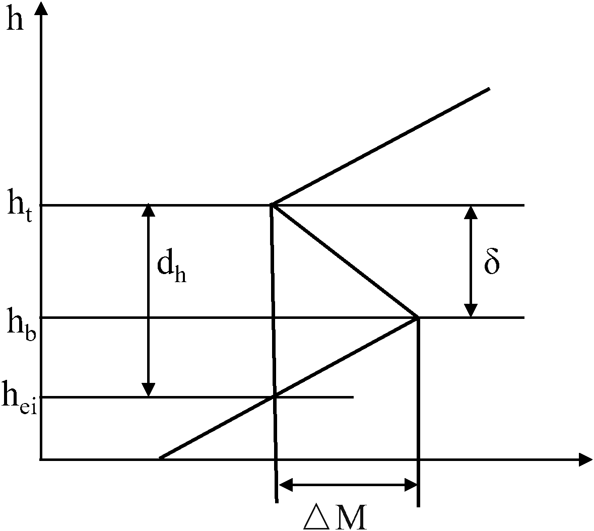
The modified refractivity profile for an elevated duct.
The thickness of elevated ducts plays a critical role in radio wave propagation loss. Thinner ducts exhibit weaker confinement of electromagnetic waves, leading to increased signal leakage and higher propagation losses. In contrast, thicker ducts significantly reduce radio wave attenuation and enhance transmission stability. Due to the pronounced spatiotemporal variability of elevated duct thickness driven by meteorological conditions, accurate prediction of duct thickness is essential for enhancing the reliability and deployment efficiency of maritime communication systems (Liu et al., 2021). Figure 2 illustrates the effect of varying duct thickness on propagation losses as a function of transmission distance at a frequency of 2GHz. The duct bottom height is held constant at 71.4m, while the duct thickness varies between 38.6m and 88.6m. The transmitting and receiving antennas are set at 105m and 150m, respectively. Assuming a maximum acceptable propagation loss of 160dB, the results indicate that thinner ducts cause a rapid increase in attenuation, thereby limiting the effective communication range. In contrast, as the duct thickness increases—particularly when the duct layer top height approaches or exceeds the height of the receiving antenna—propagation losses decrease significantly, thereby improving communication performance. Notably, the communication range reaches its maximum at a duct thickness of 88.6m, corresponding to a duct top height of 160m.
Figure 2
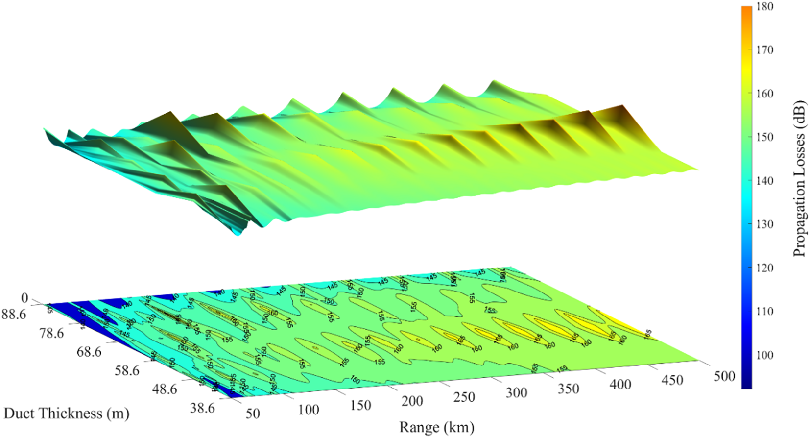
Propagation losses with distances and duct thickness at 2 GHz.
2.2 Datasets
This paper selected high vertical resolution radiosonde data (HVRRD) from US high-altitude stations to support the diagnosis and modeling of elevated ducts, as shown in Figure 3. Three geographically dispersed stations were chosen for subsequent model analysis and validation: SAN JUAN (18.43°N, 66.00°W), TRUK INTL (7.46°N, 151.85°E), and MAJURO (7.06°N, 171.23°E). These stations were selected considering both geographical and meteorological representativeness to ensure the spatial generalization of the proposed model. Specifically, the SAN JUAN station located in the Atlantic region was used to verify the model’s feasibility, while the TRUK INTL and MAJURO stations in the Pacific region were used for robustness verification. All three stations provide long-term, high-resolution, and high-quality radiosonde observations, which are conducive to verifying the cross-regional applicability of elevated duct prediction performance. The dataset was obtained from the Stratosphere-Troposphere Processes and their Role in Climate (SPARC) Data Centre (https://www.sparc-climate.org/data-centre/data-access/us-radiosonde/, accessed October 2024). This dataset covers the process through which the National Oceanic and Atmospheric Administration (NOAA) gradually upgraded its high-altitude stations from the Microcomputer-based Automatic Radio Theodolite (MicroART) radiosonde tracking system to the Radiosonde Replacement System, which employs Global Positioning System tracking. Consequently, the SPARC dataset transitioned from the MicroART format, with a temporal resolution of 6 seconds, to the RRS format, which provides enhanced sampling at a 1-second resolution (Huang et al., 2022). This upgrade in temporal resolution greatly improves the vertical continuity of the refractivity profile, enabling more accurate identification of weak and thin elevated ducts that might be missed at coarser resolutions. Compared with the 6-second MicroART data, the 1-second RRS observations capture finer-scale refractivity variations and reduce interpolation uncertainty in estimating duct boundaries. Therefore, the higher temporal resolution provides more reliable and physically consistent data for duct characterization and subsequent modeling applications.
Figure 3
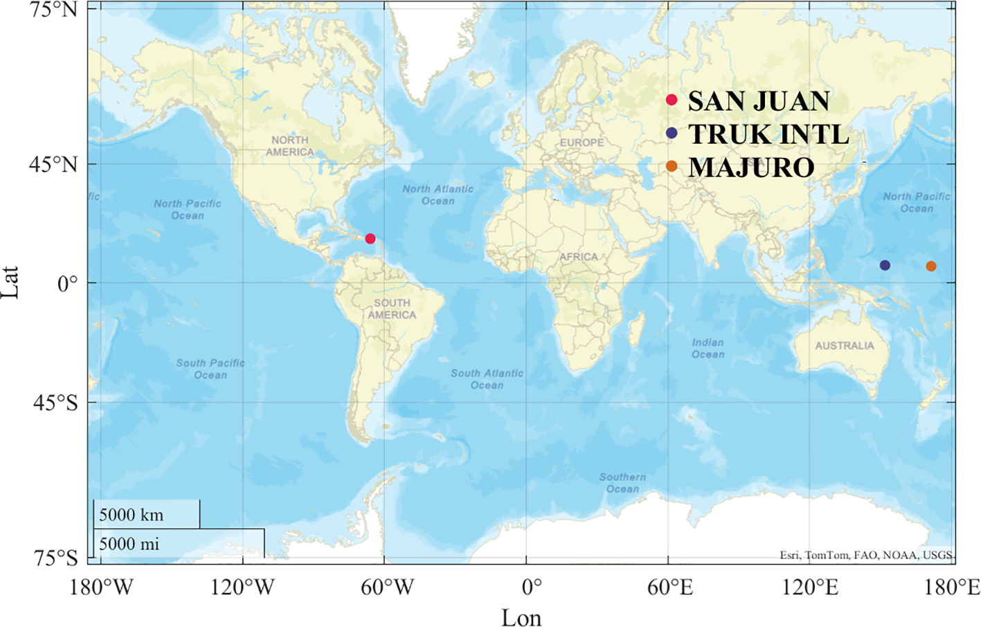
Geographic distribution of US upper-air stations and selected stations for elevated duct analysis.
2.3 Data processing
To ensure data reliability, missing values and anomalies caused by radiosonde measurement errors were removed, including missing observation times, abrupt changes in duct thickness between adjacent moments, and inconsistencies between duct thickness and duct top height trends. These missing or abnormal values were corrected by filling in the observation data from the same time on the previous day to maintain data accuracy and temporal consistency.
During the statistical processing of elevated duct samples, a two-dimensional linear interpolation method was applied to estimate duct thickness based on the modified refractivity profile. In cases where multiple elevated ducts were identified within a single profile, only the one with the most significant duct thickness was retained, along with its corresponding physical parameters such as humidity and pressure. These preprocessing steps ensure that the model input time series is constructed as continuous and physically representative data, improving the integrity and validity of the training samples.
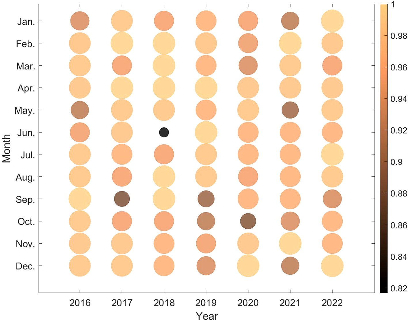
A detailed quality assessment of the SPARC dataset indicates two primary types of outliers: (1) extreme duct thickness values exceeding the physically reasonable limits (>1000m) and (2) anomalous reductions in duct thickness correlated with decreasing duct height, often resulting from radiosonde measurement inaccuracies or abrupt atmospheric disturbances. Based on this quality assessment, data preprocessing was conducted to ensure data reliability. Figure 4 presents the monthly data availability rate of radiosonde observations collected at the SAN JUAN station (18.43°N, 66.00°W) from 2016 to 2022. The availability was evaluated based on data anomalies caused by instrument malfunctions or environmental interferences within each month. To quantitatively assess the reliability of the duct data, a metric termed Data Availability Probability (DAP) is introduced, which is mathematically expressed as shown in Equation 2:
Figure 4
Data availability at SAN JUAN Station from 2016 to 2022.
where represents the total number of samples within the month, indicates the number of abnormal samples identified during that period.
The DAP value approaching 100% reflects a higher data quality and reliability level. DAP is visualized through color mapping and bubble area, with lighter shades and larger diameters indicating higher DAP levels. As shown in Figure 4, except for June 2018, when DAP dropped to 82%, the value remained above 90% in all other months. The high and stable DAP value ensured the temporal continuity of the duct parameters and provided reliable data support for model training.
Next, we conducted a statistical analysis of the distribution characteristics of elevated duct thickness at the SAN JUAN station from 2016 to 2022. As shown in Figure 5, each colored box represents the annual distribution of elevated duct thickness from 2016 to 2022, the duct thickness exhibited a broad distribution range, generally spanning from 10 m to 560m. Most observations were concentrated in the 0–200m interval, with the median consistently falling within the 100–150m range. Although year-to-year differences exist, the overall annual distributions remain relatively stable without a clear interannual trend. Each year has varying numbers of high-thickness outliers, reflecting the high-frequency, large-amplitude fluctuation characteristics of elevated ducts over time.
Figure 5
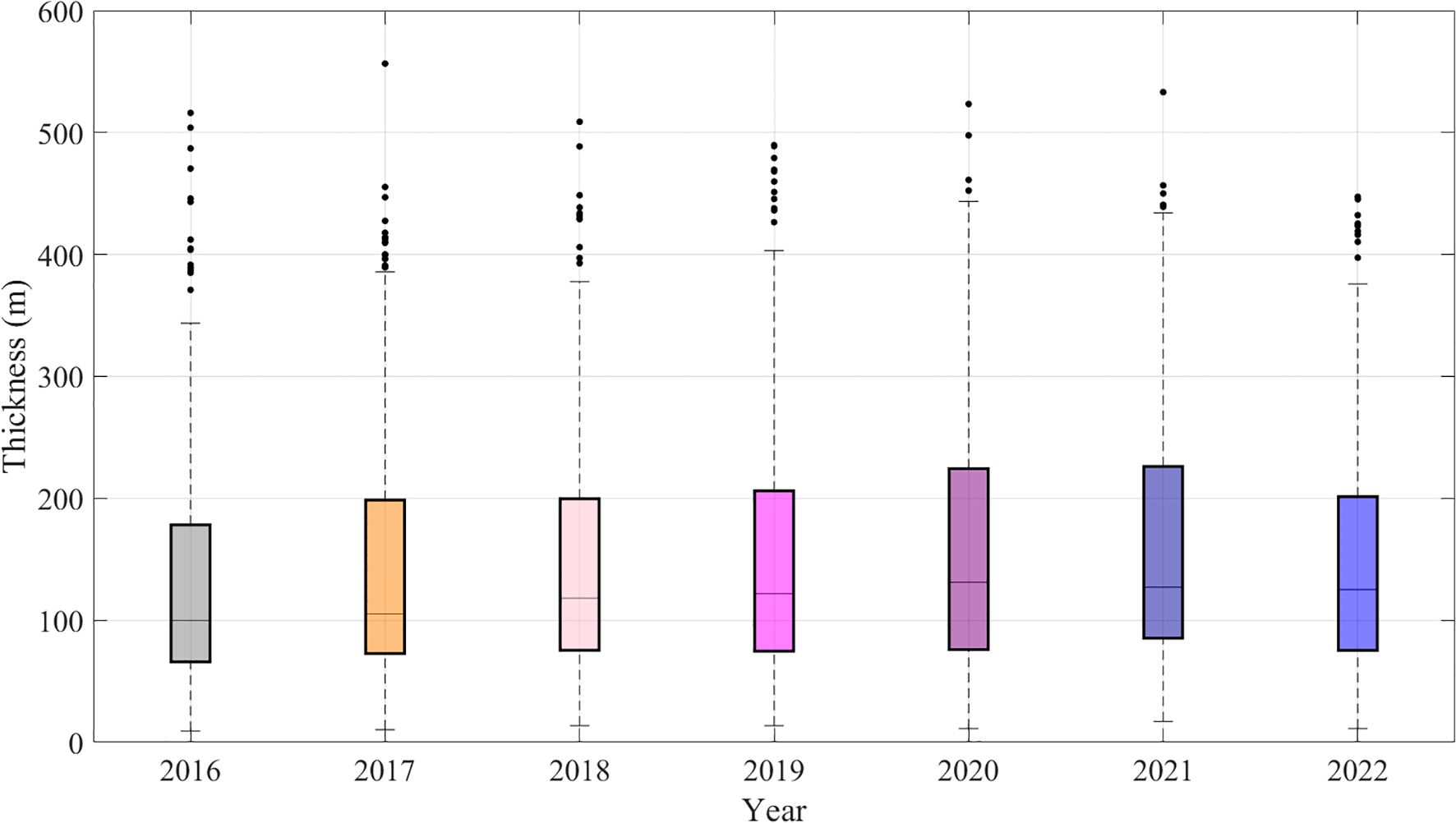
Distribution statistics of elevated duct thickness observed at the SAN JUAN station from 2016 to 2022.
3 Methods and model
3.1 Modeling idea
The thickness of elevated ducts directly affects the propagation path, transmission loss, and coverage of tropospheric radio waves. Accurately predicting duct thickness is critical for design and performance assessment of communication system. To enhance the accuracy of long-term elevated duct thickness prediction, this study proposes a prediction model that integrates CEEMDAN, TVF-EMD, and TCN using observation data from the SAN JUAN station. The model’s hyperparameters are optimized through a grid search method.
The modeling framework proposed in this study comprises three key stages: data preparation, model training, and performance evaluation, as illustrated in Figure 6.
Figure 6
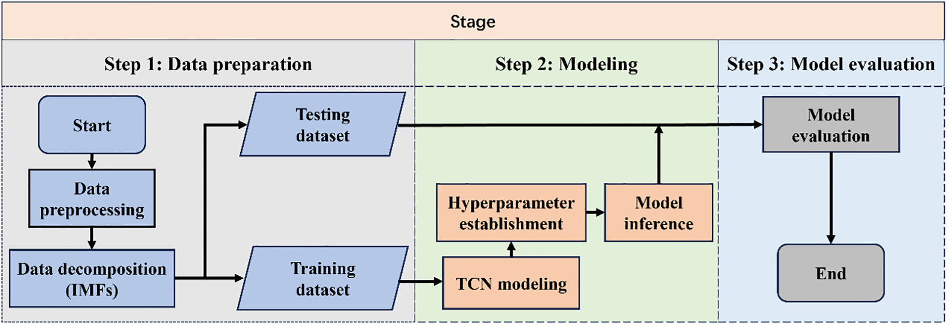
Modeling flowchart based on the CEEMDAN–TVF-EMD–TCN.
Step 1: Data preparation. The raw observational data are first preprocessed to improve data quality and ensure usability. Then, decomposition techniques are employed to extract Intrinsic Mode Functions (IMFs). The resulting dataset is divided into training and testing subsets for model fitting and validation.
Step 2: Modeling. A Temporal Convolutional Network (TCN) model is developed using the training set, and its performance is further enhanced through hyperparameter tuning. After constructing the model, the testing set generates predictions and obtains the corresponding forecast results.
Step 3: Model evaluation. The predicted values are compared with the observed data, and appropriate evaluation metrics are applied to assess the model’s performance, thereby verifying the effectiveness and robustness of the proposed approach.
3.2 CEEMDAN-TVF-EMD algorithm
The elevated duct thickness time series observed at the SAN JUAN station exhibits high-frequency and large amplitude fluctuations. This pronounced non-stationarity may interfere with the model’s capture of the underlying temporal structure, thereby reducing prediction accuracy. To enhance the model’s predictive performance, the original time series was subjected to two-stage decomposition, as shown in Table 1, to minimize sequence complexity and improve feature separability.
Table 1
| No. | Decomposition method | Function |
|---|---|---|
| 1 | CEEMDAN | CEEMDAN is a decomposition method derived from empirical mode decomposition (EMD), well-suited for processing time series characterized by non-stationarity and high-frequency disturbances (Boudraa and Cexus, 2007). Due to the significant multi-scale fluctuations in elevated duct thickness under complex meteorological conditions, traditional methods often fail to effectively extract its intrinsic structures. CEEMDAN is introduced to perform preliminary decomposition of the duct thickness time series, obtaining intrinsic mode functions (IMFs) arranged from high to low frequency (e.g., IMF1, IMF2, IMF3, etc.), along with a residual component, thereby suppressing mode aliasing and enhancing the model’s response to transient changes in duct thickness and local disturbances (Torres et al., 2011). |
| (3) | ||
| where X(t) represents the original duct thickness series, represents the i-th mode, and r(t) represents the final residual component. | ||
| 2 | TVF-EMD | TVF-EMD is a time-frequency analysis method that captures variations in signal frequency over time (Li et al., 2017). After CEEMDAN decomposition of the duct thickness time series, IMF1 and IMF2 exhibited pronounced high-frequency fluctuations and complex structures, which led to poor predictive performance when modeled directly. To enhance the time-frequency characterization of high-frequency components in the duct thickness time series and improve prediction accuracy, TVF-EMD was employed to perform secondary decomposition of IMF1 and IMF2. |
| (4) | ||
| where represents the j-th subcomponent of extracted by TVF-EMD. |
Decomposition algorithm.
3.3 TCN network
The Temporal Convolutional Network (TCN) model is designed based on the architecture of Convolutional Neural Networks (CNNs) and is applied to time series prediction tasks (Wei et al., 2022; Hewage et al., 2020). TCN effectively mitigates the gradient vanishing problem that can lead to unstable training and exhibits superior computational efficiency and extended memory retention. Figure 7 illustrates the overall architecture of the TCN, where (a) depicts the dilated causal convolution structure and (b) shows the residual connections employed between layers.
Figure 7
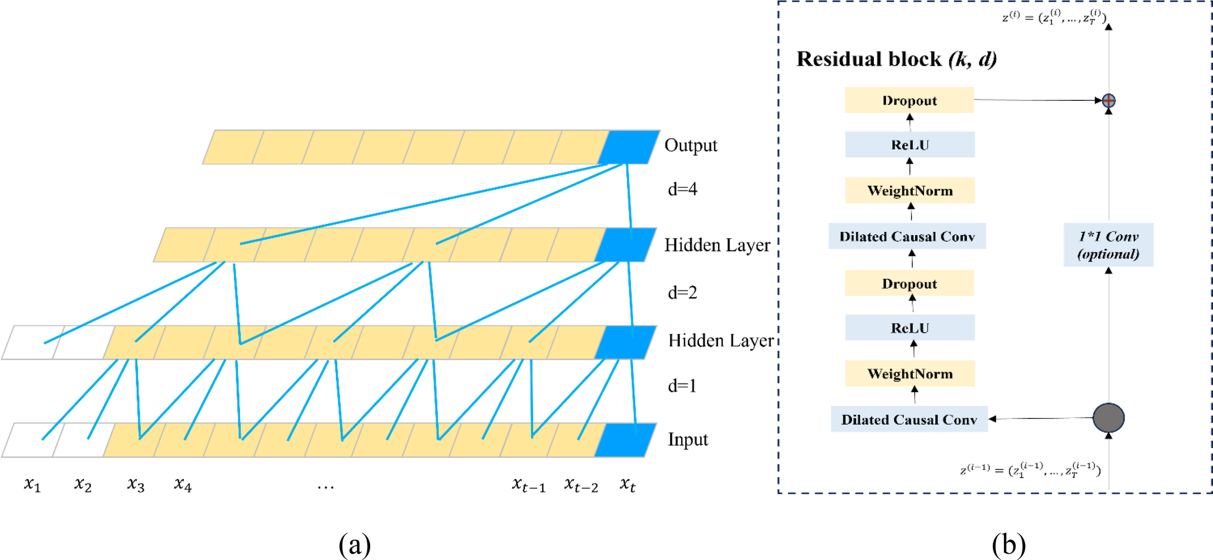
Architecture of TCN. (a) Dilated causal convolution; (b) Residual block.
A key characteristic of TCN is its use of dilated causal convolution, which ensures that an input sequence of length N yields an output sequence of the same length while preventing any information leakage from future time steps (Lea et al., 2016). In this study, the TCN module consists of two hidden convolutional layers.
The dilated convolution is defined in Equation 5:
where denotes the output of the s-th neuron in the TCN; K represents the kernel size; and d is the dilation factor. When d = 3, the dilated convolution reduces to a regular convolution.
3.4 Modeling
To enable accurate long-term prediction of duct thickness, it is essential to construct stable training samples based on historical observations and to extract temporal dependencies within the time series to support subsequent predictive modeling. This study employs time-series data from the SAN JUAN station in the United States, spanning the period from 2016 to 2022, as the sample dataset. To ensure time continuity in the predictions and enhance the model’s reference value for future applications, data from 2016 to 2020 are used as the training set, while data from 2021 to 2022 serve as the test set to validate the model’s prediction accuracy (Shi et al., 2023; Javeed et al., 2018).
Figure 8 illustrates the combinatorial forecasting process of the CEEMDAN-TVF-EMD-TCN model, and the corresponding modeling steps are outlined in Algorithm 1, as follows:
Figure 8
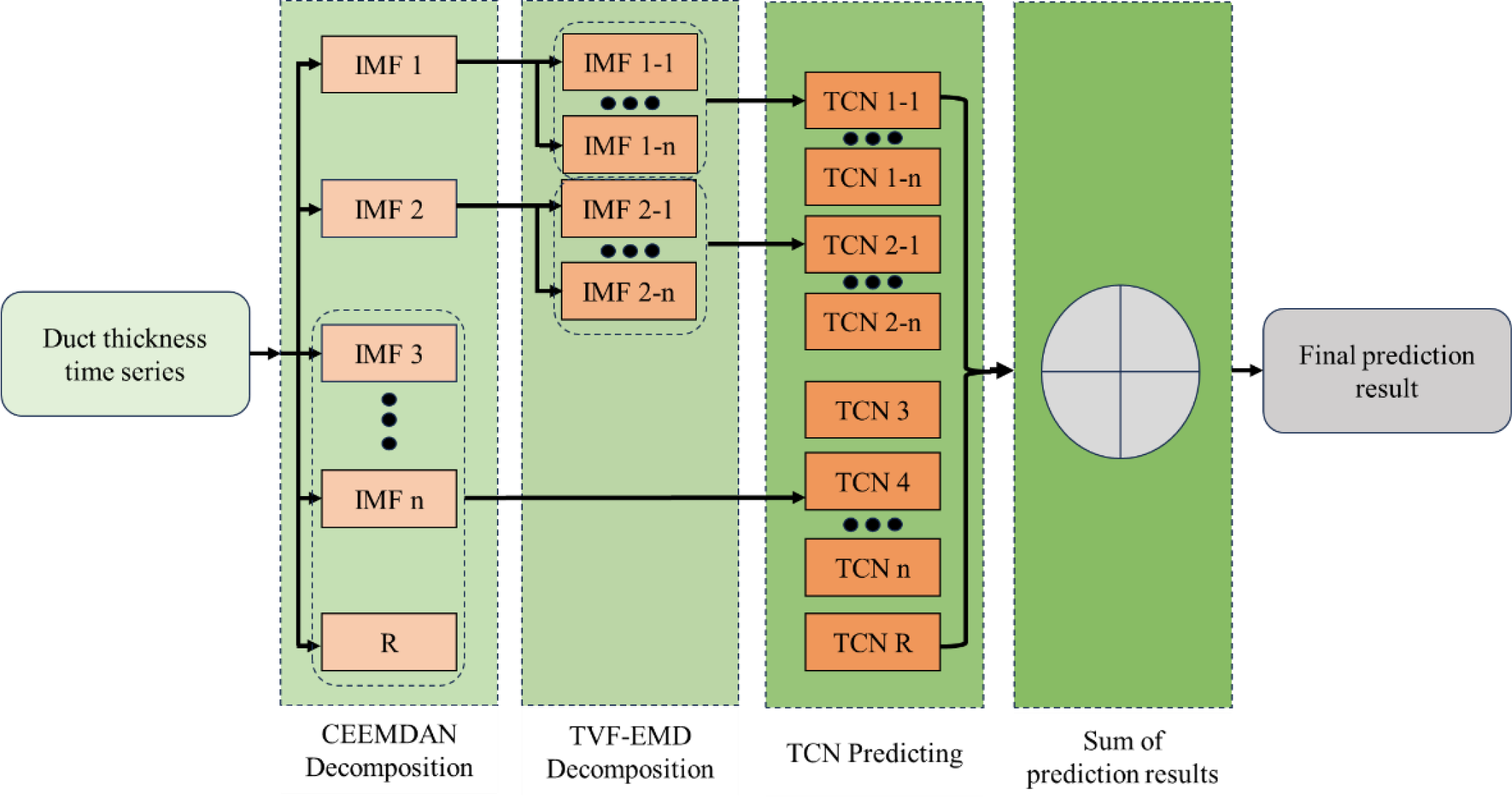
The predictive architecture of the CEEMDAN-TVF-EMD-TCN model.
Algorithm 1
Modeling steps: CEEMDAN–TVF–EMD–TCN.
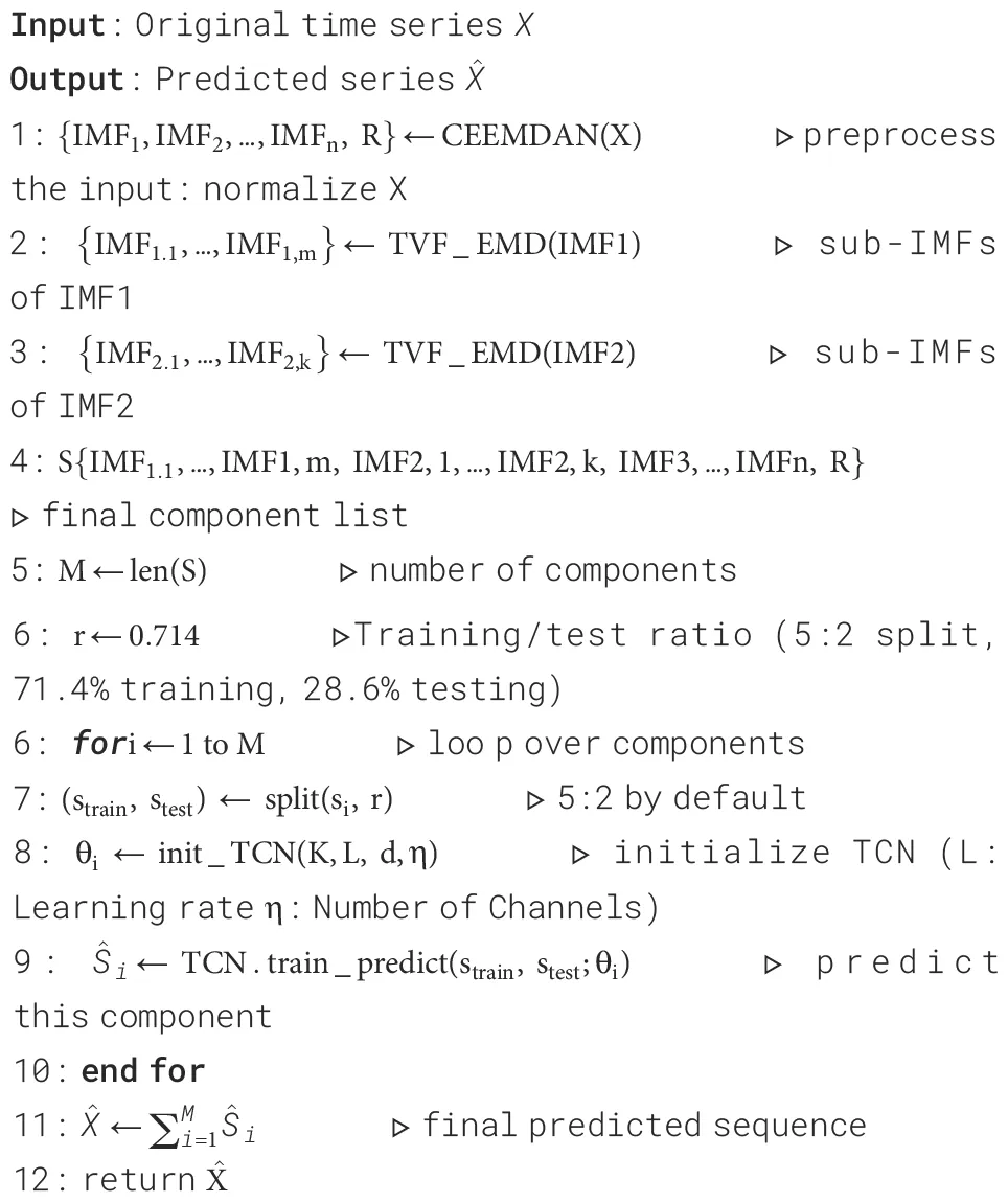
According to the decomposition principle of CEEMDAN and TVF-EMD, each IMF component represents a distinct frequency contribution within the duct-thickness time series. The high-frequency IMFs primarily capture short-term fluctuations caused by transient meteorological disturbances, while the low-frequency IMFs and the residual term describe the long-term evolution of atmospheric structures. This multi-scale decomposition separates transient variations from persistent trends, providing physically interpretable components that facilitate subsequent model learning.
To enhance the predictive performance of the CEEMDAN-TVF-EMD-TCN model, a grid search method is employed to systematically optimize four key hyperparameters: kernel size, learning rate, maximum epochs, and the number of channels (Ataei and Osanloo, 2004). Specifically, the kernel size is searched over the range [2, 3, 4, 5] with a step of 1; the learning rate is explored within [0.002, 0.004,…, 0.02] in increments of 0.002; the maximum epochs are tuned within the range [100, 110,…, 200] with a step size of 10. The number of channels was selected from three typical structures [8 16 8], [16 32 16], and [32 64 32] for the search. The model uses daily elevated duct thickness observations recorded at 00:00 UTC at the station from 2016 to 2022. A sliding-window strategy is adopted, in which the previous 24 consecutive observations serve as the input sequence and the model predicts the thickness at the next day, forming a one-step-ahead forecasting setup. Based on the experimental results, the optimal parameters listed in Table 2 were ultimately selected to construct the prediction model, and model training and test set predictions were completed based on the SAN JUAN station dataset.
Table 2
| Parameter | Parameter settings |
|---|---|
| Kernel size | 3 |
| Learning rate | 0.006 |
| Max Epochs | 160 |
| Number of Channels | [16 32 16] |
Modeling parameters.
The CEEMDAN-TVF-EMD dual decomposition module down-converts the original time series via modal separation, effectively suppressing high-frequency noise and extracting dominant trend components (Li et al., 2017). While this preprocessing step increases computational complexity slightly, it substantially improves signal quality and stability, thereby enhancing the TCN model’s predictive performance. (Guo C. et al., 2023; Wang et al., 2014).
For the prediction stage, this study quantifies the TCN’s computational complexity using floating-point operations (FLOPs). According to the standard definition, FLOPs measure the total number of floating-point calculations in a forward pass (Chen et al., 2023). The computational cost of a one-dimensional convolution is calculated as follows:
where L denotes the sequence length, K is the kernel size, and and represent the numbers of input and output channels.
In our setting (L = 24, K = 3, channels = [16 32 16]), each single-input TCN requires FLOPs. For N IMFs obtained from the CEEMDAN–TVF-EMD dual decomposition, the total computational cost of the model is FLOPs. For typical N values observed in the experiments (ranging from 14 to 20), the overall computation remains modest, and the resulting accuracy improvement demonstrates that the proposed framework achieves a reasonable balance between model complexity and predictive performance (Guo R. et al., 2023; Bai et al., 2018).
4 Results and discussion
This study employs Mean Absolute Error (MAE) and Root-Mean-Square Error (RMSE) to assess the CEEMDAN-TVF-EMD-TCN model’s accuracy and robustness.
1. MAE: Measures the absolute deviation between the predicted values and observed values , it is less sensitive to outliers.
2. RMSE: Measures the sample standard deviation between the predicted values and the observed values , reflecting the degree of dispersion. A lower RMSE indicates better performance, particularly in nonlinear fitting.
In Equations 7 and 8, n denotes the number of samples.
4.1 Model validation
This section presents the training and validation of the CEEMDAN-TVF-EMD-TCN model using observational data from the SAN JUAN station during the period 2016–2022. The data from 2016 to 2020 served as the training set, and data from 2021 to 2022 served as the test set. The definitions of the evaluation metrics are provided in Equations 6 and 7. The CEEMDAN-TVF-EMD-TCN model yields an MAE of 12.8m and an RMSE of 16.3m.
Figure 9 shows the comparison between observed and predicted elevated duct thickness values at the SAN JUAN station for the years 2021 and 2022. The blue bars indicate the absolute prediction errors for each day. It shows that:
Figure 9
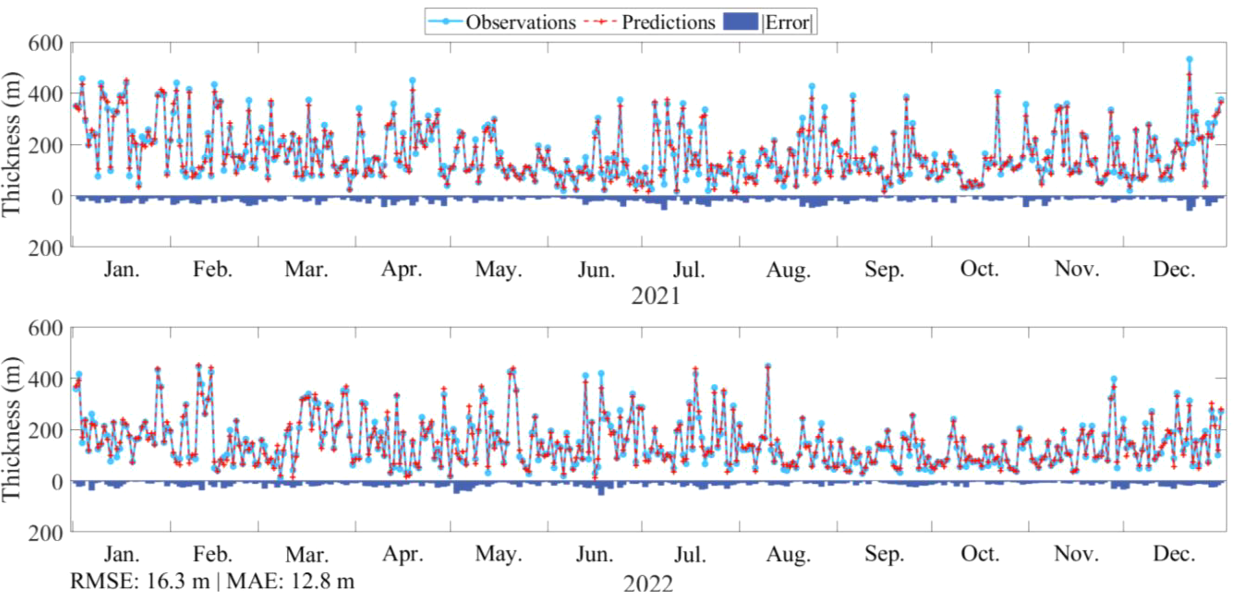
Prediction results at the SAN JUAN station.
-
The predicted and observed values possess a high degree of consistency in the overall trend, which indicates that the model can capture the changing pattern of the duct thickness well.
-
At peak points (e.g., July and August in 2021), the predictions are generally lower than the observed values, with the blue bars showing a significant increase in error. This underestimation pattern during peak periods suggests there is still room for improvement in the model to handle the extreme case of rapid changes in duct thickness. However, the overall error level is still within reasonable limits.
-
The model demonstrates strong predictive performance from January to April and October to December, characterized by low forecast errors. In contrast, forecast errors increase from May to September, coinciding with higher volatility levels. Nevertheless, even during periods of heightened volatility, the model consistently captures the overall trend, demonstrating enhanced adaptability and robustness in handling complex temporal patterns.
To account for the significant influence of monsoons on elevated ducts, April and October, months characterized by distinctly different climatic features, are selected as representative periods for comparative analysis. Figure 10 shows the observed and predicted duct thickness values, along with the corresponding absolute prediction errors for April and October 2022. The following conclusions can be drawn from Figure 10:
Figure 10
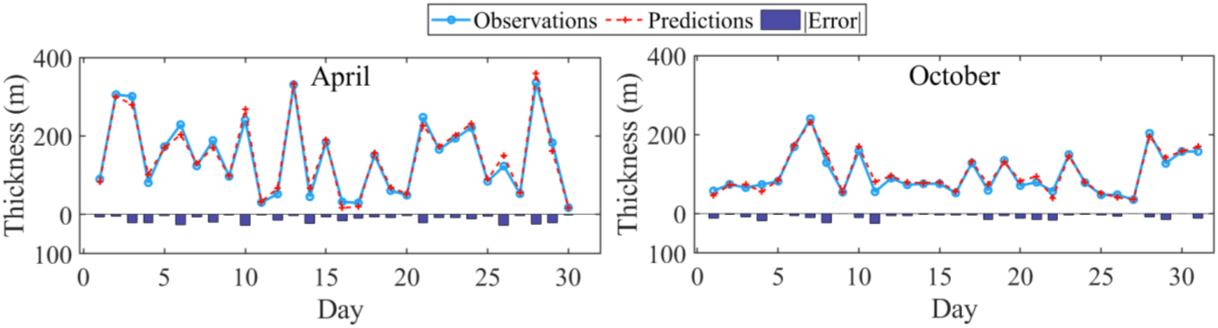
Prediction results for April and October 2022 at the SAN JUAN Station.
-
During April, the duct thickness exhibits marked fluctuations characterized by alternating peaks and troughs, with maximum values exceeding 350m and minimum values approaching 0m, indicating pronounced non-stationarity. These abrupt short-term variations substantially increase the modeling complexity, resulting in noticeably elevated prediction errors during these intervals and demonstrating a decline in forecasting accuracy under intense perturbation conditions.
-
During October, the overall fluctuation in duct thickness remained within the range of 100–250m, particularly from mid- to late-month, when the variations became more gradual, exhibiting either steady increases or slow declines. At this stage, the model predictions closely matched the observed values, and the prediction errors were substantially reduced, suggesting that the model performs better in terms of time-series fitting and generalization under stable meteorological conditions.
-
The CEEMDAN-TVF-EMD-TCN model shows strong adaptability under different seasonal conditions. In April, the duct thickness fluctuates drastically, and the model maintains good trend-tracking ability; in October, the duct thickness changes steadily, and the prediction accuracy is significantly improved. These results highlight the model’s robustness and reliability under varying atmospheric conditions.
Figure 11 presents the monthly distribution of prediction errors at the SAN JUAN station throughout 2022. The figure aggregates the absolute prediction errors by calendar month, illustrating the temporal variation in forecasting accuracy on a monthly scale. From Figure 11, we can deduce the following:
Figure 11
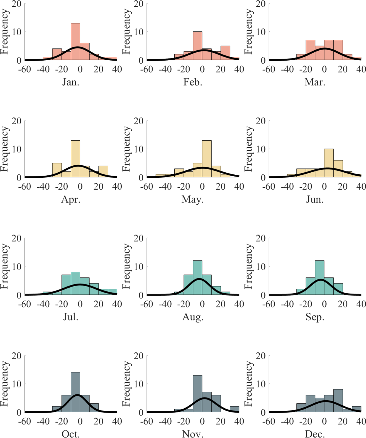
Monthly error statistics of duct thickness predictions at SAN JUAN station (2022).
-
Most prediction errors fall within ±20m, demonstrating that the CEEMDAN-TVF-EMD-TCN model maintains low error levels throughout the year. Notably, in October and November, the error distribution is most concentrated, indicating superior fitting accuracy and stability even during autumn, a season with highly variable meteorological conditions.
-
In months such as April, May, and September, the error distribution exhibits a slight skew toward negative values, indicating a tendency of the model to underestimate duct thickness. This bias may be attributed to abrupt fluctuations in duct structure or complex meteorological conditions that the model does not fully capture.
Building upon the monthly prediction performance presented in Figures 11, 12 employs box plots further to depict the distribution of prediction errors across different months. This analysis provides deeper insight into the magnitude and dispersion of the model’s errors, enabling a more comprehensive evaluation of its seasonal stability and overall reliability.
Figure 12
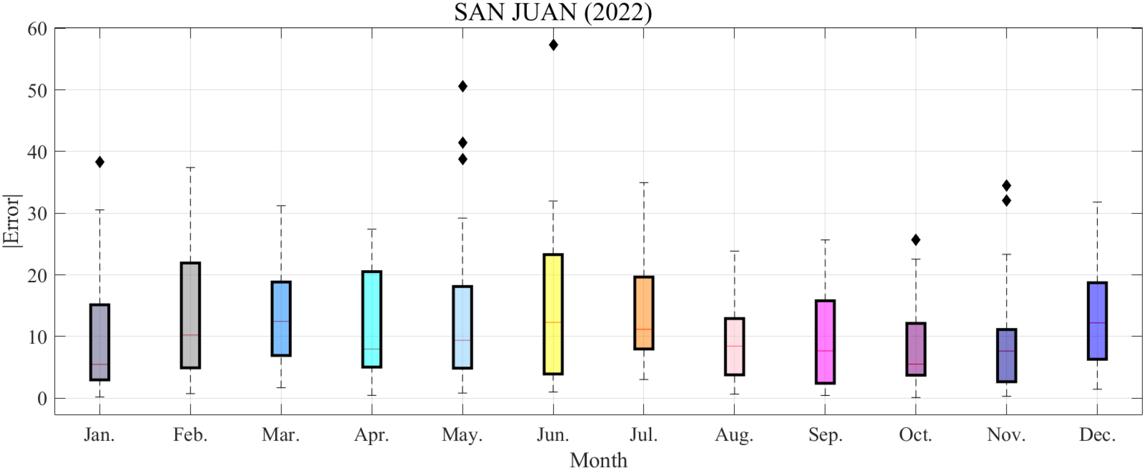
Error distribution of elevated duct thickness predictions at the SAN JUAN station in 2022.
The following observations can be drawn from Figure 12.
-
The absolute median values of prediction errors across months from January to December are 5.48, 10.25, 12.45, 7.96, 9.38, 12.29, 11.16, 8.44, 7.67, 5.54, 7.64, and 12.22 m, respectively. The monthly median errors range from 5.48m to 12.45m, showing moderate variability. The highest median error occurred in March (12.45m), while relatively lower values were observed in January (5.48m) and October (5.54m). The median errors in the remaining months were relatively consistent.
-
The interquartile range (IQR) values for each month from January through December are as follows: 12.17, 17.00, 11.91, 15.47, 13.25, 19.36, 11.67, 9.14, 13.39, 8.41, 8.46, and 12.41 m. The monthly interquartile ranges (IQRs) fall from 8.41m to 19.36m. Among these, the IQR values are relatively higher in June (19.36m) and February (17.00m), suggesting a greater dispersion of errors during these months. In contrast, the lower IQR values observed in October (8.41m), November (8.46m), and August (9.14m) indicate a comparatively more concentrated error distribution.
-
In October and November, the median prediction errors are relatively lower—5.54 m and 7.64 m, respectively—with the corresponding IQR being the weakest of the year (8.41 m and 8.46 m). These results indicate that the model exhibits more minor prediction deviations during this period and produces a more concentrated error distribution, reflecting superior overall forecasting stability. In contrast, the median errors in March and June exceed 12 m, and their IQRs remain consistently high throughout the year, revealing that the prediction errors during these months are larger and more volatile. Consequently, the model’s stability and accuracy are relatively weaker in March and June. The model demonstrates a relatively stable performance from late summer to autumn (August–November).
4.2 Comparison analysis
The above results demonstrate that the proposed CEEMDAN-TVF-EMD-TCN hybrid model achieves high forecasting accuracy at the SAN JUAN station. To further assess the generalization capability of the proposed approach across different regions, cross-station forecasting experiments were conducted at two additional stations: MAJURO and TRUK INTL. The training and test sets of the model for each station are divided in the same way as Section 3. Figure 13 displays the prediction results for the MAJURO and TRUK INTL stations. Subfigures (a) and (b) present the comparisons between observed and predicted values at MAJURO for 2021 and 2022, respectively, while subfigures (c) and (d) show the corresponding comparisons for TRUK INTL in the same years.
Figure 13
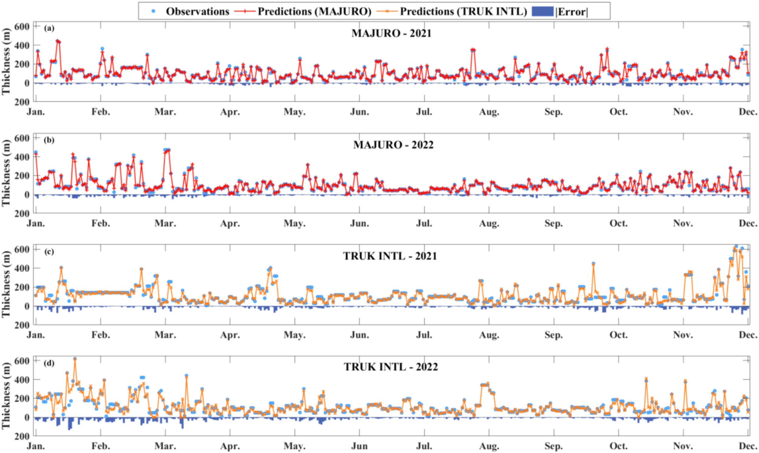
Regional analysis results at the MAJURO and TRUK INTL Stations.
Three conclusions can be drawn from Figure 13:
-
At the MAJURO station, the model performs well overall, accurately capturing the variation in duct thickness. In spring and winter, when thickness fluctuations are more pronounced, the predictions closely follow the observed values, reflecting the model’s sensitivity to abrupt changes. During summer and autumn months, prediction errors are minimal, demonstrating strong fitting capability under relatively calm atmospheric conditions.
-
At the TRUK INTL station, the model effectively captures the annual variation in duct thickness, with low prediction errors and stable performance during the summer and autumn. However, instances of lag and overestimation are observed in spring and late-year periods, suggesting that the model’s responsiveness to abrupt fluctuations in duct thickness could be further improved.
-
The results indicate that the CEEMDAN-TVF-EMD-TCN hybrid modeling approach proposed in this study performs well across the MAJURO and TRUK INTL stations, demonstrating good cross-station applicability. Nonetheless, localized prediction biases remain during periods of high fluctuation, suggesting that further refinement of the modeling process could enhance its robustness and generalization when handling extreme disturbance patterns.
To further evaluate the accuracy of duct thickness predictions across different seasons, this study uses the 2022 prediction results as data samples and compares the RMSE values at the two stations during spring, summer, and autumn, thereby assessing the seasonal adaptability and stability of the proposed model. Here, a year is divided into four seasons: March-May is spring, June-August is summer, and autumn includes September, October, and November.
Figure 14 shows the RMSE values for each season at the MAJURO and TRUK INTL stations. The following three conclusions can be drawn from Figure 14:
Figure 14
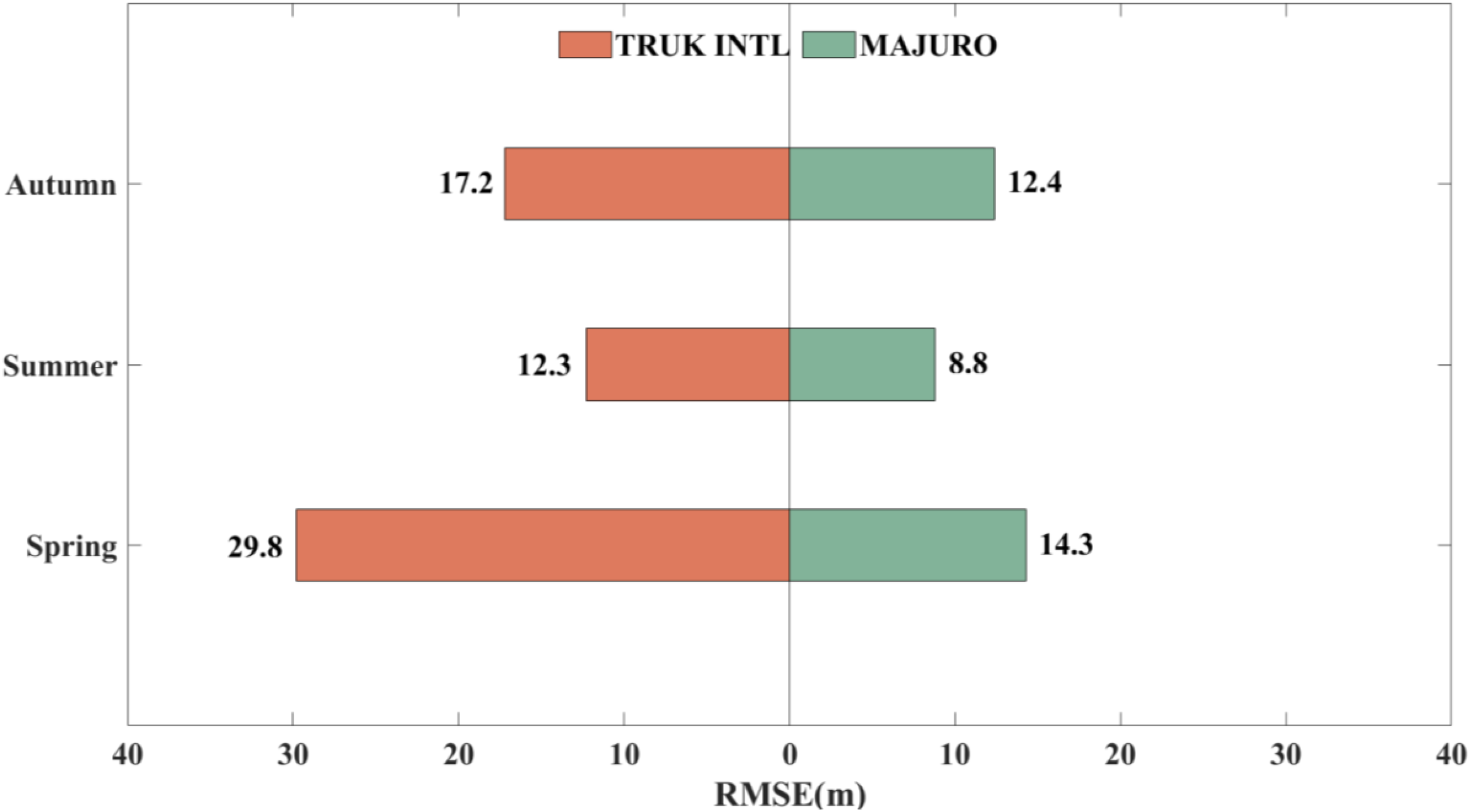
Seasonal analysis results in 2022 at the MAJURO and TRUK INTL stations.
-
At the TRUK INTL station, the RMSE increased markedly in spring, reaching 29.8m—the highest value recorded throughout the year. This seasonal spike in RMSE suggests that the model’s predictive performance during spring was adversely affected, potentially due to complex meteorological conditions or heightened variability in the input data.
-
The model maintained stable performance at the MAJURO station, with RMSE ranging from 8.8m to 14.3m. The prediction errors remained relatively low, particularly during summer and autumn, reflecting consistent model reliability at this station.
-
Overall, the model performed consistently during summer and autumn, with RMSE remaining relatively low. RMSE was relatively high in spring, especially at the TRUK INTL station, reaching 29.8 m, which may be attributed to stronger atmospheric instability and frequent convective activity in spring, leading to more irregular refractivity profiles and larger prediction uncertainties. In contrast, the relatively stable stratification in summer reduces refractivity fluctuations and results in lower model errors. The RMSE differences between stations suggest that the model’s ability to adapt to station-specific characteristics still requires further improvement for broader geographical applicability.
5 Conclusions
A TCN long-term predicting model based on CEEMDAN-TVF-EMD is proposed for a time series of elevated duct thickness with nonlinear and non-stationary characteristics. Leveraging high-resolution radiosonde observations, the model effectively captures fine-scale variations in duct thickness and enhances its responsiveness to short-term atmospheric perturbations. Based on the TCN model, this method improves the modeling ability of long-term dependencies in time-series data. The CEEMDAN-TVF-EMD double decomposition algorithm was introduced to predict elevated duct features, extending one-dimensional time series data to a multi-dimensional feature space, significantly reducing data complexity, and enhancing feature expression capabilities. This study uses the elevated duct thickness data from the SAN JUAN station as model input. Each component of the hybrid model contributes distinctively to its predictive performance: CEEMDAN reduces high-frequency noise and mitigates non-stationarity; TVF-EMD refines decomposed signals and strengthens their time–frequency representation; and TCN captures long-term temporal dependencies and nonlinear relationships among the reconstructed features. As a result, the CEEMDAN-TVF-EMD-TCN model effectively analyzes the nonlinear and non-stationary characteristics of elevated duct thickness data and provides accurate long-term prediction values, with cross-station experiments further confirming its strong generalization capability. Significantly, the hybrid model relies solely on the elevated duct thickness time series without auxiliary meteorological or physical parameters, reflecting its high forecasting efficiency and practical applicability. This study develops a deep learning model based on two-stage decomposition to improve the prediction accuracy of elevated duct thickness. However, the current work remains primarily data-driven and does not explicitly address the underlying physical mechanisms governing elevated duct formation, and its generalization capability has been validated at only a limited number of stations. In addition, the validation experiment was conducted in low-latitude maritime regions. Future work will involve testing in mid- and high-latitude marine environments to further validate the model’s accuracy. Future work will further validate the model’s spatial generalization capabilities across additional observation stations. At the same time, physical mechanism–oriented modeling will be explored by incorporating key meteorological and environmental parameters to enhance the interpretability and physical relevance of the proposed hybrid model.
Statements
Data availability statement
The original contributions presented in the study are included in the article/Supplementary Material. Further inquiries can be directed to the corresponding author.
Author contributions
CZY: Visualization, Conceptualization, Methodology, Validation, Software, Formal analysis, Writing – original draft. JW: Conceptualization, Resources, Supervision, Writing – review & editing, Funding acquisition, Writing – original draft. CY: Project administration, Validation, Writing – review & editing, Investigation, Funding acquisition. WL: Data curation, Writing – review & editing. JL: Writing – review & editing, Validation.
Funding
The author(s) declared that financial support was received for this work and/or its publication. This research was funded in part by the National Natural Science Foundation of China (No. 62031008) and in part by the Basic Scientific Research Program of China (No. JSHS2024210A001).
Conflict of interest
The authors declared that this work was conducted in the absence of any commercial or financial relationships that could be construed as a potential conflict of interest.
Generative AI statement
The author(s) declared that generative AI was not used in the creation of this manuscript.
Any alternative text (alt text) provided alongside figures in this article has been generated by Frontiers with the support of artificial intelligence and reasonable efforts have been made to ensure accuracy, including review by the authors wherever possible. If you identify any issues, please contact us.
Publisher’s note
All claims expressed in this article are solely those of the authors and do not necessarily represent those of their affiliated organizations, or those of the publisher, the editors and the reviewers. Any product that may be evaluated in this article, or claim that may be made by its manufacturer, is not guaranteed or endorsed by the publisher.
Supplementary material
The Supplementary Material for this article can be found online at: https://www.frontiersin.org/articles/10.3389/fmars.2025.1730671/full#supplementary-material
References
1
Alappattu D. P. Wang Q. (2016). “ Evaporation and Elevated Duct Properties over the Subtropical Eastern Pacific Ocean Region Using MAGIC Data,” in 2016 United States National Committee of URSI National Radio Science Meeting (USNC-URSI NRSM)(Boulder, CO, USA: IEEE), 1–2. doi: 10.1109/USNC-URSI-NRSM.2016.7436231
2
Ataei M. Osanloo M. (2004). Using a combination of genetic algorithm and the grid search method to determine optimum cutoff grades of multiple metal deposits. Int. J. Surf. Min. Reclam. Environ.18, 60–78. doi: 10.1076/ijsm.18.1.60.23543
3
Bai S. Kolter J. Z. Koltun V. (2018). An empirical evaluation of generic convolutional and recurrent networks for sequence modeling. arXiv preprint arXiv:1803.01271. doi: 10.48550/arXiv.1803.01271
4
Boudraa A.-O. Cexus J.-C. (2007). EMD-based signal filtering. IEEE Trans. Instrum. Meas.56, 2196–2202. doi: 10.1109/TIM.2007.907967
5
Chen J. Hao H. Shiu-hong K. (2023). “ Run, don't walk: chasing higher FLOPS for faster neural networks,” in 2023 IEEE/CVF Conference on Computer Vision and Pattern Recognition (CVPR), Vancouver, BC, Canada, June 18–22. 12021–12031, I EEE, Piscataway, NJ, USA. doi: 10.1109/CVPR52729.2023.01231
6
Cheng Y. Zhong W. Zhao B. (2024). Study on elevated duct prediction model of the south China sea based on radiosonde data. Mar. Forecasts.41, 44–52. doi: 10.11737/j.issn.1003-0239.2024.06.005
7
Cheng Y. Zhou S. Wang D. (2013). Review of the study of atmospheric ducts over the sea. Adv. Earth Sci.28, 318. doi: 10.11867/j.issn.1001-8166.2013.03.0318
8
Fowdur T. P. Doorgakant B. (2023). A review of machine learning techniques for enhanced energy efficient 5G and 6G communications. Eng. Appl. Artif. Intell.122, 106032. doi: 10.1016/j.engappai.2023.106032
9
Franklin K. B. Wang Q. Jiang Q. Shen L. (2022). Understanding evaporation duct variabilities on turbulent eddy scales. J. Geophys. Res-atmos.127, e2022JD036434. doi: 10.1029/2022JD036434
10
Guo C. Kang X. Xiong J. (2023). A new time series forecasting model based on complete ensemble empirical mode decomposition with adaptive noise and temporal convolutional network. Neural Process. Lett.55, 4397–4417, IEEE, Piscataway, NJ, USA. doi: 10.1007/s11063-022-11046-7 , PMID:
11
Guo R. Zhang H. Zhang Y. Jiang X. (2023). Prediction of PM2.5 concentration based on the CEEMDAN-RLMD-BiLSTM-LEC model. PeerJ.11, e15931. doi: 10.7717/peerj.15931 , PMID:
12
Han J. Wu J. Zhang L. Wang H. Zhu Q. Zhang C. (2022). A classifying-inversion method of offshore atmospheric duct parameters using AIS data based on artificial intelligence. Remote Sens.14, 3197. doi: 10.3390/rs14133197
13
Hao X. (2022). Research on the Statistical Characteristic, Inversion and Prediction of Tropospheric Refraction Parameters. Xidian University, Xi’an, China. doi: 10.27389/d.cnki.gxadu.2022.000072
14
Hewage P. Behera A. Trovati M. Pereira E. Ghahremani M. Liu Y. (2020). Temporal convolutional neural (TCN) network for an effective weather forecasting using time-series data from the local weather station. Soft Comput.24, 16453–16482. doi: 10.1007/s00500-020-04954-0
15
Hu W. Liu C. Lin F. Zhang Y. Guo X. (2021). Characteristics of atmospheric ducts and its impacts on FM broadcasting in wuhan. Chin. J. Radio Sci.35, 856–867. doi: 10.13443/j.cjors.2020071402
16
Huang L. Zhao X. Liu Y. (2022). The statistical characteristics of atmospheric ducts observed over stations in different regions of american mainland based on high-resolution GPS radiosonde soundings. Front. Environ. Sci.10. doi: 10.3389/fenvs.2022.946226
17
Javeed S. Alimgeer K. S. Javed W. Atif M. Uddin M. (2018). A modified artificial neural network based prediction technique for tropospheric radio refractivity. PloS One13, e0192069. doi: 10.1371/journal.pone.0192069 , PMID:
18
Jordan M. S. Durkee P. A. (2000). Verification and Validation of the Satellite Marine-Layer/Elevated Duct Height (SMDH) Technique. Naval Postgraduate School, Monterey, CA, USA.
19
Lea C. Vidal R. Reiter A. Hager G. D. (2016). “ Temporal convolutional networks: A unified approach to action segmentation,” in Computer Vision – ECCV 2016 Workshops (LNCS 9915). Springer, Cham, 47–54. doi: 10.1007/978-3-319-49409-8_7
20
Li H. Li Z. Mo W. (2017). A time varying filter approach for empirical mode decomposition. IEEE Trans. Signal Process.138, 146–158. doi: 10.1016/j.sigpro.2017.03.019
21
Liu F. Pan J. Zhou X. Li G. Y. (2021). Atmospheric ducting effect in wireless communications: challenges and opportunities. J. Commun. Inf. Networks6, 101–109. doi: 10.23919/JCIN.2021.9475120
22
Liu W. Wang J. Yang C. (2024). “ A short-term forecasting model of elevated duct based on the long short-term memory network,” in 2024 IEEE 12th Asia-Pacific Conference on Antennas and Propagation (APCAP), IEEE, Piscataway, NJ, USA,Nanjing, China. 1–2. doi: 10.1109/APCAP62011.2024.10881664
23
McBride M. B. (2000). “Estimation of Stratocumulus-Topped Boundary Layer Depth Using Sea Surface and Remotely Sensed Cloud-Top Temperatures. Naval Postgraduate School, Monterey, CA, USA.
24
Shi Y. Yang C. Wang J. Zhang Z. Meng F. Bai H. (2023). A forecasting model of ionospheric foF2 using the LSTM network based on ICEEMDAN decomposition. IEEE Trans. Geosci. Remote Sens.61, 1–16. doi: 10.1109/TGRS.2023.3336934
25
Tepecik C. Navruz L. (2018). A novel hybrid model for inversion problem of atmospheric refractivity estimation. AEU-Int. J. Electron.84, 258–264. doi: 10.1016/j.aeue.2017.12.009
26
Torres M. E. Colominas M. A. Schlotthauer G. Flandrin P. (2011). A Complete Ensemble Empirical Mode Decomposition with Adaptive Noise. In Proceedings of the 2011 IEEE International Conference on Acoustics, Speech and Signal Processing (ICASSP), Prague, Czech Republic, pp. 4144–4147. IEEE, Piscataway, NJ, USA.
27
Wang J. Liu W. Yang C. (2025). UAV-Aided Maritime Communication over the Pacific Ocean Using the Elevated Duct toward Future Wireless Networks. Sci. Rep.15, 11920. doi: 10.1038/s41598-025-90065-5 , PMID:
28
Wang J. Yang C. Yan N. (2021). Study on digital twin channel for the B5G and 6G communication. Chin. J. Radio Sci.36, 340–48, 385. doi: 10.12265/j.cjors.2020240
29
Wang Y.-H. Yeh C.-H. Young H.-W. V. Hu K. Lo M.-T. (2014). On the computational complexity of the empirical mode decomposition algorithm. Physica A.400, 159–167. doi: 10.1016/j.physa.2014.01.020
30
Wei Z. Wu J. Yin B. Jia D. Xu J. (2022). “ Atmospheric duct propagation loss prediction based on time convolution network (TCN),” in 2022 International Conference on Wireless Communications, Electrical Engineering and Automation, Indianapolis, IN, USA. 152–158, IEEE, Piscataway, NJ, USA. doi: 10.1109/WCEEA56458.2022.00039
31
Yang N. Su D. Wang T. (2023). Atmospheric ducts and their electromagnetic propagation characteristics in the northwestern south China sea. Remote Sens.15, 3317. doi: 10.3390/rs15133317
32
Yang C. Wang J. (2022). The investigation of cooperation diversity for communication exploiting evaporation ducts in the south China sea. IEEE Trans. Antennas Propag.70, 8337–8347. doi: 10.1109/TAP.2022.3177509
33
Zhang Y. Guo X. Zhao Q. Zhao Z. Kang S. (2020). Research status and thinking of atmospheric duct. Chin. J. Radio Sci.35, 813–831. doi: 10.13443/j.cjors.2020072401
34
Zhang B. Yan K. Hui B. Huang Q. Gao H. (2024). “ Real-time atmospheric duct height prediction framework based on spatio-temporal to ensure maritime communication security,” in Proceedings of the International Conference on Wireless Artificial Intelligent Computing Systems and Applications, Qingdao, China. 241–253. Springer, Cham. doi: 10.1007/978-3-031-71467-2_20
35
Zhao X. Wang D. Huang K. Huang K. Chen J. (2013). Statistical estimations of atmospheric duct over the south China sea and the tropical eastern Indian ocean. Chin. Sci. Bull.58, 2794–2797. doi: 10.1007/s11434-013-5942-8
36
Zhu M. Atkinson B. W. (2005). Simulated climatology of atmospheric ducts over the persian gulf. Bound.-Layer Meteorol.115, 433–452. doi: 10.1007/s10546-004-1428-1
Summary
Keywords
elevated duct, thickness, predicting, CEEMDAN, TVF-EMD, TCN
Citation
Yao C, Wang J, Yang C, Liu W and Liao J (2026) CEEMDAN-TVF-EMD-TCN based method for elevated duct parameters predicting with high-resolution radiosonde data. Front. Mar. Sci. 12:1730671. doi: 10.3389/fmars.2025.1730671
Received
23 October 2025
Revised
17 November 2025
Accepted
28 November 2025
Published
05 January 2026
Volume
12 - 2025
Edited by
Ranjit Kumar Paul, Indian Council of Agricultural Research (ICAR), India
Reviewed by
Hanjie Ji, Xidian University, China
Hong-guang Wang, China Research Institute of Radiowave Propagation, China
Updates
Copyright
© 2026 Yao, Wang, Yang, Liu and Liao.
This is an open-access article distributed under the terms of the Creative Commons Attribution License (CC BY). The use, distribution or reproduction in other forums is permitted, provided the original author(s) and the copyright owner(s) are credited and that the original publication in this journal is cited, in accordance with accepted academic practice. No use, distribution or reproduction is permitted which does not comply with these terms.
*Correspondence: Cheng Yang, ych2041@tju.edu.cn
Disclaimer
All claims expressed in this article are solely those of the authors and do not necessarily represent those of their affiliated organizations, or those of the publisher, the editors and the reviewers. Any product that may be evaluated in this article or claim that may be made by its manufacturer is not guaranteed or endorsed by the publisher.