Abstract
Introduction:
Ocean wave conditions forecasting is crucial for reducing wave-related disasters and enhancing prevention and mitigation capabilities in China's coastal regions.
Methods:
This study develops a convolutional neural network (CNN) model optimized by a random search algorithm to predict significant wave height (Hs) and mean wave period (Tm). Using SWAN nearshore wave simulation data as input, the model analyzes the impact of different historical input step lengths and various forecast lead times on prediction performance. It is applied to the Yantai Fishing Zone, China.
Results:
The optimal input step length for the model is 3 hours, achieving correlation coefficients (CC) of 0.9997 for Hs and 0.9969 for Tm. The mean absolute errors (MAE) are 0.0075 m and 0.0562 s, and the root mean square errors (RMSE) are 0.0149 m and 0.2014 s, respectively. Based on the 3-hour input step length, forecasts were conducted for lead times of 3, 6, 9, and 12 hours. As the forecast lead time increased, prediction accuracy declined, but the model still effectively captured the main trends of Hs and Tm.
Discussion:
The model errors remain within an acceptable range, and its computational efficiency is significantly superior to traditional numerical methods. This demonstrates the model's good applicability in the study area, indicating its potential to effectively enhance fishery production efficiency and optimize fishing operation scheduling.
1 Introduction
Ocean wave disasters are one of the main marine hazards affecting China, endangering the lives of coastal city residents, causing significant economic losses, hindering the development of coastal cities, damaging offshore platforms, and affecting maritime transport (Fang et al., 2017; Zheng et al., 2023; Zhang et al., 2024). According to the Bulletin of China Marine Disaster (2023), there were 28 destructive wave events recorded in China’s coastal waters during that year, resulting in 8 fatalities and direct economic losses of approximately 26 million yuan. Between 2014 and 2023, an average of 35.6 destructive wave events occurred annually, causing an average of 26 deaths and direct economic losses of about 32 million yuan per year. Achieving accurate and efficient ocean wave forecasting has become a hot topic in marine research. Accurate wave conditions forecasting helps guide normal marine activities, reduces the adverse impacts of wave disasters on human production and life, ensures the safety of maritime activities, and enhances disaster prevention and mitigation capabilities in China’s coastal areas (Ali et al., 2024; Chen et al., 2025).
Traditional ocean wave forecasting methods primarily rely on numerical forecasting models developed based on the spectral energy balance equation, mainly including Wave Modeling (WAM) (Group, 1988), the Simulating Waves Nearshore (SWAN) model (Booij et al., 1999), and the WAVEWATCH III model based on WAM (Tolman and Chalikov, 1996; Tolman et al., 2002). Through extensive research and long-term development, numerical models have achieved operational implementation, contributing to improved accuracy in wave forecasting in marine environments. However, high-resolution forecasting for local sea areas is limited by the computational complexity of these models, often requiring high computational costs and significant time (Zilong et al., 2022; Halicki et al., 2025). This makes it challenging to meet the rapid response needs under extreme weather conditions, affecting real-time decision-making activities such as planning maritime construction operation windows and determining the timing of personnel evacuation from offshore platforms.
With the continuous development and progress of artificial intelligence technology, intelligent forecasting is becoming increasingly mature. Machine learning and deep learning algorithms are continuously iterating and updating. Due to their strong adaptive learning and nonlinear mapping capabilities, many scholars are applying them in various research fields, demonstrating powerful forecasting abilities and good forecasting effects (Zuo et al., 2019; Qiu et al., 2023; Xia and Wang, 2024; Sharma et al., 2025). In the field of intelligent ocean wave forecasting, research primarily focuses on fixed offshore locations, utilizing historical marine observation data to predict wave parameters through machine learning or deep learning methods (Oh and Suh, 2018; Meng et al., 2021). Tsai et al. (2002) used an artificial neural network (ANN) model to learn the interconnection weights among wave data from three stations at Taichung Harbor in central Taiwan, enabling the forecast or supplementation of wave data at target stations based on data from adjacent stations during the inference phase, with good model performance. Mandal and Prabaharan (2006) employed a Nonlinear Autoregressive with exogeneous inputs (NARX) recurrent neural networks with the resilient propagation (Rprop) update algorithm to forecast wave heights at 3, 6, and 12 hours using observed wave data near India’s west coast, achieving correlation coefficients of 0.95, 0.90, and 0.87, respectively, indicating better performance compared to previous studies. Deka and Prahlada (2012) applied discrete wavelet transform to decompose wave height into multi-frequency data, which was used as input for an ANN model to forecast Hs at different times near India’s west coast, with the hybrid model demonstrating superior forecast performance and consistency compared to the standalone ANN model. Hao et al. (2022) developed an EMD-LSTM model combining Long Short-Term Memory (LSTM) neural networks and empirical mode decomposition (EMD) to forecast Hs at three locations offshore China, significantly improving prediction accuracy compared to the standalone LSTM model and effectively mitigating the impact of non-stationarity on wave forecasting performance. HHuang et al. (2024a) developed a long-term AI forecasting model based on a channel-independent patch time series transformer model (PatchTST), using wave reanalysis data from four locations. With a prediction horizon of 720 hours, the model demonstrated superior accuracy and effectiveness in predicting long-term significant wave height compared to the Informer, LSTM, and NeuralProphet models. Halicki et al. explored the effectiveness of Recurrent Artificial Neural Networks for short-term Hs predictions using limited Baltic Sea buoy data. Through hyperparameter optimization and regularization techniques, their approach extended prediction horizons to 12 hours, demonstrating significant improvements in accuracy and reliability compared to conventional forecasting methods (Halicki et al., 2025).
For two-dimensional ocean wave field forecasting, due to the scarcity of wave observation stations and the high cost of their deployment, datasets commonly utilize reanalysis data or numerical model data for constructing intelligent forecasting models (Zhou et al., 2021; Gao et al., 2023; Liu et al., 2024). Bai et al. (2022) developed a CNN model integrated with a random search algorithm using ECMWF Reanalysis v5 (ERA5) data for Hs forecasting in the South China Sea, achieving a mean absolute percentage error (MAPE) of 19.48% for 72-hour forecasts, with satisfactory performance. HHuang et al. (2024b) proposed an AI model utilizing an improved Spatio-Temporal Identity (STID) algorithm to predict coastal wave spatiotemporal evolution. The model demonstrates robust adaptability to complex topography and effectively captures the global spatiotemporal dependencies of wave evolution across different regions. Results indicate that the model can be applied to more accurately simulate the spatiotemporal evolution process of coastal waves. Yu et al. (2024) developed a multi-attention trajectory gated recurrent unit (MA-TrajGRU) model using SWAN wave data, combining the TrajGRU algorithm with a multi-attention mechanism for wave forecasting in the South China Sea, demonstrating good performance suitable for 24-hour Hs forecasts. Li et al. (2024) calibrated the SWAN parameterization scheme and used its outputs to train a spatiotemporal forecasting model combining self-attention mechanisms and Convolutional LSTM (ConvLSTM), improving the prediction accuracy of Hs in the East China Sea. Scala et al. employed a Conv-LSTM model using bathymetric, wind fields, wave fields data, and wave buoy measurements to predict the significant wave height, peak period, and wave direction in the Mediterranean Sea for the next 24 hours. The results demonstrated that the model exhibits high accuracy in forecasting short-term wave variations and can more effectively capture the characteristics of wave crest changes (Scala et al., 2025). To better demonstrate the advancements in intelligent wave forecasting, we have summarized the relevant developments in Table 1.
Table 1
| Forecast type | Year | Author(s) | Forecast model |
|---|---|---|---|
| Fixed offshore locations | 2002 | Tsai et al. | ANN |
| 2006 | Mandal et al. | NARX | |
| 2012 | Deka et al. | Wavelet Neural Network(WLNN) | |
| 2022 | Hao et al. | EMD-LSTM | |
| 2024 | Huang et al. | PatchTST | |
| 2025 | Halicki et al. | AR, ARIMA, LSTM | |
| Two-dimensional ocean wave field | 2021 | Zhou S et al. | ConvLSTM |
| 2022 | Bai G et al. | CNN | |
| 2023 | Gao Z et al. | Driving field forced ConvLSTM | |
| 2024 | Huang et al. | the Improved-STID algorithm | |
| 2024 | Liu Y et al. | EarthFormer | |
| 2024 | Yu M et al. | MA-TrajGRU | |
| 2024 | Li G et al. | Self-Attention ConvLSTM |
The advancements in intelligent wave forecasting.
This study first constructed a high spatiotemporal resolution dataset of Hs and Tm using the SWAN model, then employed a CNN model to conduct forecasting analysis of Hs and Tm in the Yantai Fishing Zone, aiming to develop a high spatiotemporal resolution intelligent forecasting model for rapid wave conditions forecasting in the Yantai Fishing Zone. The main contributions of this study are as follows:
-
This study utilizes the physics-based nearshore wave numerical model SWAN as a data source to develop a CNN-based intelligent wave forecasting model, achieving significant improvement in the prediction accuracy of Hs and Tm.
-
It systematically analyzes the impact of input step length on model performance and identifies an optimal input step length of 3, which notably enhances forecasting results.
-
The model’s effectiveness was validated in the Yantai Fishing Zone. The results demonstrate its ability to capture the main trends of wave parameters across various forecast lead times.
-
This method provides relevant technical references for improving marine disaster warning and mitigation capabilities in China’s coastal regions.
The structure of the remainder of the paper is as follows: Section 2 details the specific setup of the SWAN wave model, the bathymetry map of the study area, and information about the Hs and Tm dataset. Section 3 describes the detailed structure of the CNN forecasting model and the model evaluation metrics. Section 4 analyzes the impact of different input step lengths on the model’s forecasting results and evaluates the model’s performance at various forecast lead times based on the optimal input step length. Section 5 presents the conclusions, discussing the strengths and limitations of the current model as well as future research directions.
2 Data and methods
2.1 Data
2.1.1 SWAN wave model setup
SWAN (Simulating WAves Nearshore) is a third-generation numerical wave model developed and maintained by Delft University of Technology (Booij et al., 1999). It solves the wave action balance equation in the spectral domain and is capable of modeling wave generation, propagation, and dissipation in coastal and shallow water environments. Due to its robustness and adaptability, SWAN has been extensively applied in wave simulations associated with tropical cyclones or extratropical weather processes, such as cold fronts, mid-latitude storms, or winter monsoon events.
The offshore bathymetry required for the SWAN model is derived from the ETOPO1 global bathymetry dataset (https://ngdc.noaa.gov/mgg/global/relief/ETOPO1/tiled/, accessed on 3 September 2023) with a spatial resolution of 1 arc-minute. The nearshore bathymetric data is derived from nautical chart soundings (chart numbers: C1210011, C1210012, C1411910, C1311900, C1312100, C1312300, C1311300, C1311700, C1311800). All depth data marked on the charts have been converted to depth values relative to the mean sea level (MSL) datum.
The driving wind field is derived from WRF outputs and interpolated to a horizontal resolution of 0.04°. The wind field domain covers the region from 116.5°E to 130.0°E and from 28.5°N to 42.0°N, with a temporal resolution of 1 hour. The wave simulation domain covers the region from 117°E to 128°E and from 32°N to 41°N, hourly wave characteristics were simulated for the period from 2021 to 2024, and the output variables include significant wave height, mean wave period, peak wave period and wave direction. We employed the SWAN model’s physical parameterization schemes described in Table 2.
Table 2
| Setting | SWAN domain |
|---|---|
| Domain | 117 ~ 128°E and from 32 ~ 41°N |
| Resolution | 2.5km |
| Grid size | 421×361 |
| Spectral discretization | 0.04–1.0 Hz |
| water depth | Chart Depth & Measured Depth |
| Time step | 600s |
| Wind input | Westhuysen (van der Westhuysen et al., 2007) |
| Whitecapping | AB (Alves and Banner, 2003) |
| Bottom friction | JONSWAP (Hasselmann et al., 1973) |
| Wind drag formula | FIL (Zijlema et al., 2012) |
| Wind field input | WRF |
SWAN model parameter settings and physical schemes.
2.1.2 Data validation
The model validation data are obtained from four buoy stations, covering the period from January 1 to December 31, 2024, with a temporal resolution of 1 hour. The station information and locations are shown in Table 3 and Figure 1.
Table 3
| Station | Longitude (E) | Latitude (N) | Observation Period |
|---|---|---|---|
| buoy1 | 121.43°E | 37.61°N | 2024.01.01-2024.12.31 |
| buoy2 | 120.26°E | 37.69°N | |
| buoy3 | 120.93°E | 38.41°N | |
| buoy4 | 121.38°E | 36.24°N |
Locations and time periods of observational data.
Figure 1
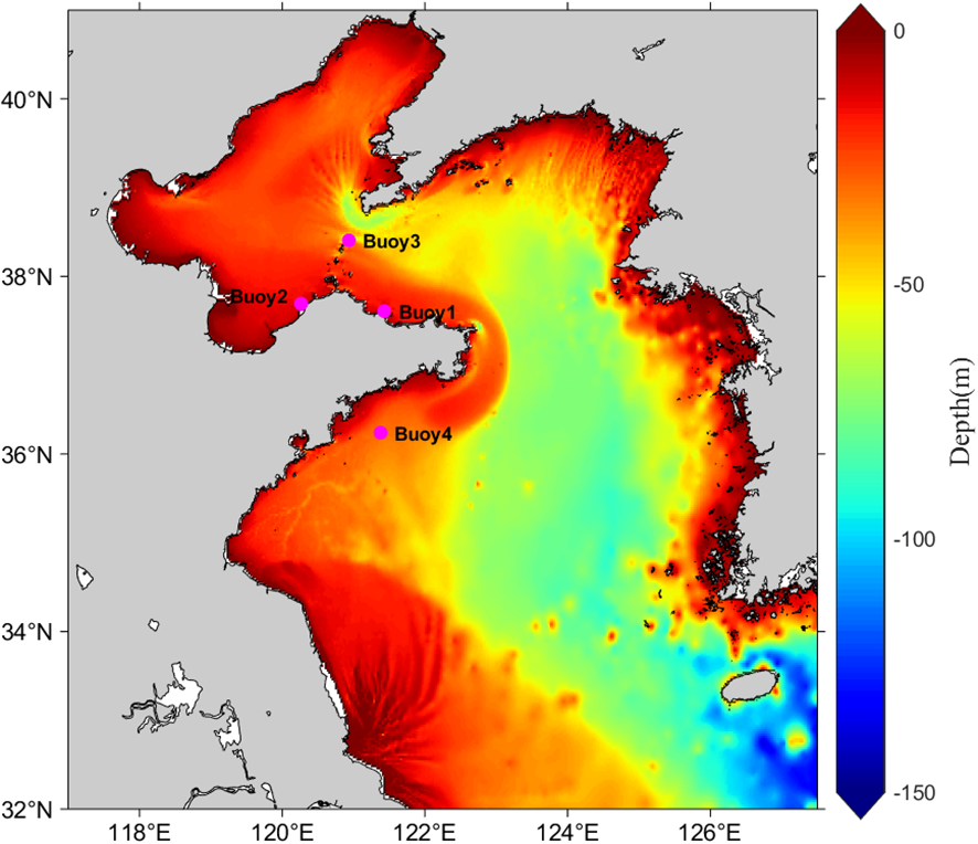
Computational domain of the SWAN model and the distribution of wave observation stations used for validation.
The MAE and RMSE of Hs and Tm are summarized in Table 4, and the comparison between hourly buoy observations and model simulations for the entire year of 2024 is shown in Figures 2, 3. Here, the x-axis represents the different month/day information in 2024. For buoy1, the MAE and RMSE of Hs are 0.149 m and 0.218 m, while the MAE and RMSE of Tm are 0.97 s and 1.14 s. For buoy2, the MAE and RMSE of Hs are 0.152 m and 0.217 m, and the MAE and RMSE of Tm are 0.93 s and 1.19 s. For buoy3, the MAE and RMSE of Hs are 0.202 m and 0.278 m, and the MAE and RMSE of Tm are 0.97 s and 1.09 s. For buoy4, the MAE and RMSE of Hs are 0.202 m and 0.278 m, and the MAE and RMSE of Tm are 0.97 s and 1.09 s.
Table 4
| Station | Metrics | Hs (m) | Tm (s) |
|---|---|---|---|
| buoy1 | MAE | 0.149 | 0.97 |
| RMSE | 0.218 | 1.14 | |
| buoy2 | MAE | 0.152 | 0.93 |
| RMSE | 0.217 | 1.09 | |
| buoy3 | MAE | 0.202 | 0.97 |
| RMSE | 0.278 | 1.09 | |
| buoy4 | MAE | 0.151 | 0.92 |
| RMSE | 0.202 | 1.08 |
MAE, RMSE of Hs and Tm.
Figure 2
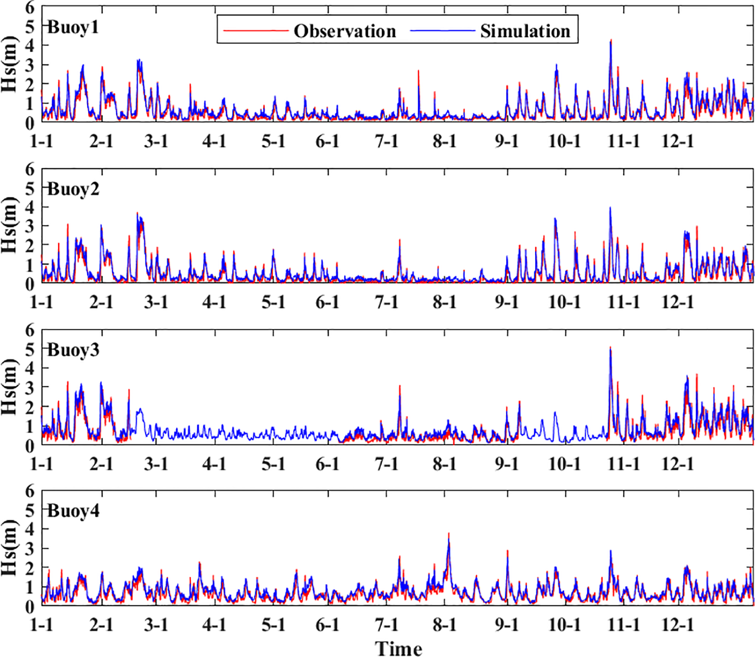
Comparisons of model forecast data and observed buoy data for Hs.
Figure 3
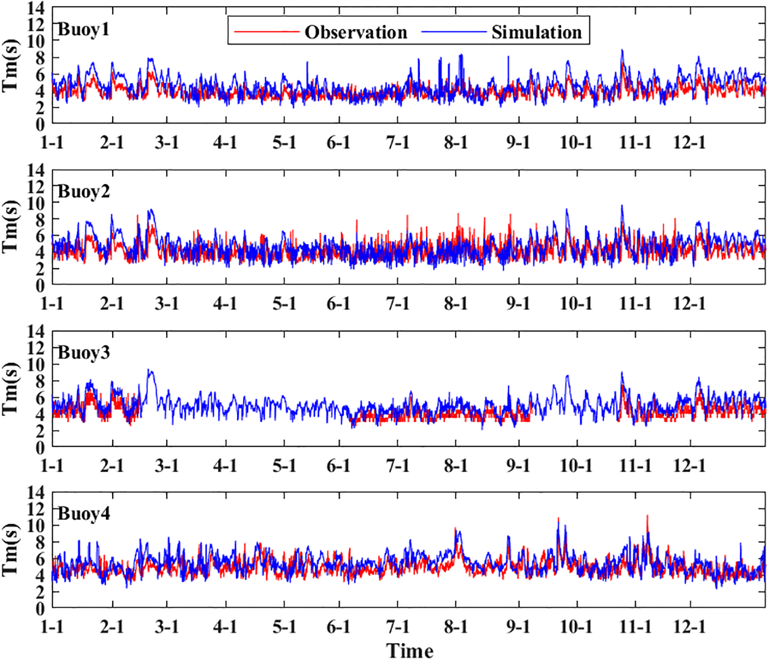
Comparisons of model forecast data and observed buoy data for Tm.
2.1.3 Study area
The dataset used in the ocean wave conditions forecasting study includes Hs and Tm. By adopting a down-sampling method based on bilinear interpolation, the SWAN data were converted into input data suitable for the CNN model, reducing the spatial resolution to 0.05° × 0.05° to balance model performance and reduce computational costs (Chen et al., 2021; Jörges et al., 2023). The temporal frequency is 1 hour, covering the period from 00:00 on January 1, 2021, to 23:00 on December 31, 2024. The study area is selected as the Yantai Fishing Zone, with a longitude range of 119° to 122.5° and a latitude range of 35.5° to 39°, which is beneficial for ensuring the safety of fishermen and vessels and improving fishery production efficiency. The bathymetry map, annual mean Hs, and annual mean Tm are shown in Figure 4. According to Figure 4, the water depth in the study area primarily ranges from 10 to 60 m, the annual mean Hs is concentrated between 0.6 m and 1.2 m, and the annual mean Tm is concentrated between approximately 2.8 s and 5.5 s.
Figure 4
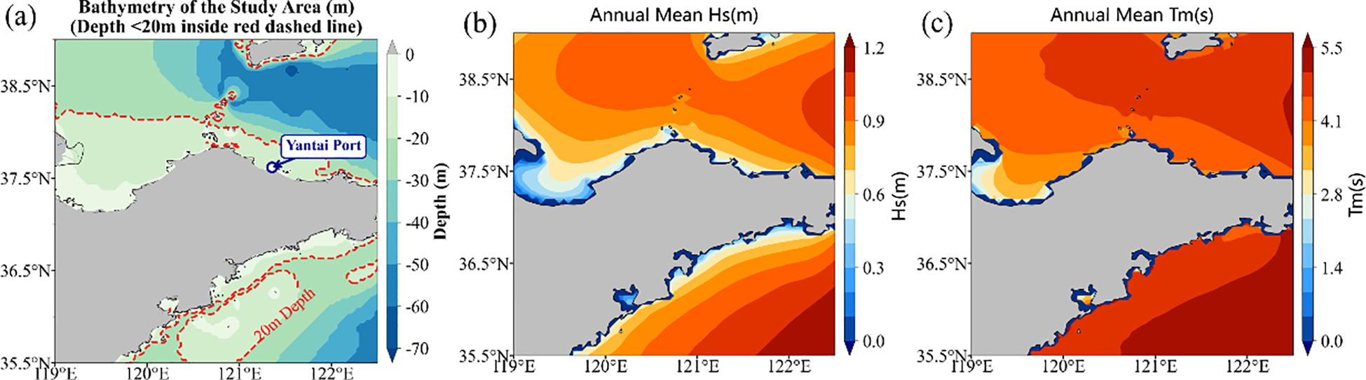
Bathymetry of the study area (a), Annual mean Hs(b), Annual mean Tm(c).
2.2 Methods
This study developed a CNN-based model to forecast Hs and Tm in the Yantai Fishing Zone. The model uses historical time steps of Hs and Tm as inputs to forecast the corresponding Hs and Tm at a specified lead time.
2.2.1 Theory of CNN
The CNN model is designed to process multi-array data and is commonly used for analyzing grid-like data such as images. Since 2000, it has been successfully applied in various fields, including biomedical image segmentation, facial recognition, and autonomous vehicle driving (Ning et al., 2005; Hadsell et al., 2009; Taigman et al., 2014; LeCun Y, 2015). Atypical CNN consists of an input layer, convolutional layers, pooling layers, and fully connected layers. The convolutional layer processes input data through convolution operations to reduce computational load. The pooling layer, including max pooling and average pooling, is primarily used for data dimensionality reduction, enhancing the model’s generalization ability, and preventing overfitting. By stacking multiple convolutional and pooling layers, CNNs can progressively extract low-level features from images, gradually forming abstract high-level feature representations.
2.2.2 Model hyper-parameter setup
In the two-dimensional regional forecasting, the use of pooling layers may lead to the loss of some wave data, reducing the model’s forecasting performance. Therefore, we chose to eliminate pooling layers and instead adopted a structure with multiple stacked convolutional layers. The CNN model was built using Keras 2.4.3 and trained and tested on a 24GB NVIDIA RTX 4090 GPU. For the original dataset, we first applied min-max normalization to scale the data to the range [0,1]. Then, the 35,064 samples were divided into training, validation, and test sets according to a 6:2:2 ratio, with the numbers of training and validation samples fixed at 21,038 and 7,013, respectively. The number of test samples was adjusted according to the model’s input step lengths and lead time, calculated by the formula: number of test samples = 7,013 – input step lengths – lead time + 1. This partition of training, validation, and test sets also applies to the baseline models described in Section 4.2. After model training, the data were denormalized to restore them to their original scale. In deep learning, model performance is highly dependent on the values of hyperparameters, which significantly impact the model’s complexity, computational speed, and other aspects, requiring careful tuning to achieve optimal performance (Bischl et al., 2023). However, manual selection of hyperparameters is time-consuming and labor-intensive. Therefore, appropriate algorithms are typically employed to enhance efficiency and ensure reproducibility. In hyperparameter optimization, grid search and random search are two commonly used methods. Grid search exhaustively evaluates all possible parameter combinations to identify the optimal hyperparameters, whereas random search abandons exhaustive traversal and instead randomly samples a fixed number of parameter combinations from the hyperparameter space for evaluation. Compared to grid search, random search offers higher computational efficiency and greater flexibility, with studies indicating that it often outperforms grid search in terms of performance (Bergstra and Bengio, 2012). Therefore, this study employs the random search algorithm from the Keras Tuner library to optimize the hyperparameters of the CNN model, with both max_trials and epochs set to 50 to ensure the identification of the optimal parameter configuration. The hyperparameter search space, as detailed in Table 5, encompasses the number of convolutional layers, the number of convolutional kernels, the learning rate, and the choice of optimizer.
Table 5
| Hyper-parameters | Range |
|---|---|
| Number of hidden layers | {2,…, 4} |
| Neurons per layer | {0, 21,…, 29} |
| Optimizer | Adam, RMSProp, SGD |
| Learning_rate | {1e-4, 1e-2} |
Hyper-parameters involved in the model establishment.
The convolutional kernel size is uniformly set to 3×3, and the ReLU activation function is employed to enhance the model’s nonlinear fitting capability and improve its expressive power. The stride in the convolution process adopts the default setting, and the “same” padding method is used to ensure that the input dimension of 71×71 remains unchanged throughout the convolution process. Finally, a convolutional layer with a 1×1 kernel is used to output the predicted values of wave height and wave period for the study area. The model’s loss function is mean squared error (MSE), with a batch size of 8. To prevent overfitting, an early stopping mechanism is introduced with a patience value of 10. Training is halted if the validation loss does not decrease for 10 consecutive epochs or when training reaches 100 epochs, and the best-performing model is saved. The model architectures with optimal hyperparameters obtained through random search are shown in Figures 5, 6. Both the Hs and Tm prediction models employ a four-layer convolutional structure, with the number of convolutional kernels configured as 80, 80, 240, 464 for the Hs model and 16, 64, 256, 160 for the Tm model. The Adam optimizer is uniformly adopted, with the learning rate set to 0.0001 for the Hs model and 0.001 for the Tm model.
Figure 5
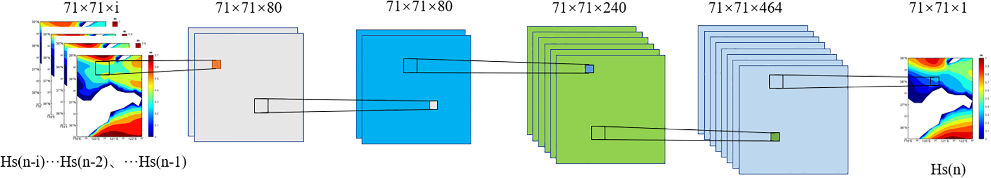
Hs forecasting model architecture diagram.
Figure 6
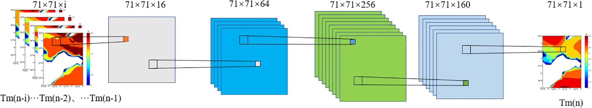
Tm forecasting model architecture diagram.
2.2.3 Evaluation metrics
We employed various evaluation metrics to analyze the performance of the CNN wave forecasting model, including MAE, RMSE, CC, spatial mean absolute error (SMAE), and spatial root mean squared error (SRMSE). The calculation of evaluation metrics is shown in Equations 1–5.
where n represents the total number of data points, denotes the one-dimensional sequence value obtained by flattening the forecasted spatiotemporal sequence (excluding land points) at the i hour, represents the mean of the one-dimensional forecasted sequence, denotes the one-dimensional sequence value obtained by flattening the true spatiotemporal sequence (excluding land points) at the i hour, and represents the mean of the one-dimensional true sequence. indicates the forecasted value at location and the t hour, and indicates the true value at location and the t hour.
3 Results
In this section, we first evaluated the forecasting performance of the constructed models for Hs and Tm with different input step lengths at the same forecasting time. Based on the analysis of the forecasting results, the optimal input step length was determined. Then, using the optimal model, we conducted forecasts and comparative analyses for Hs and Tm at different lead times.
3.1 The impact of different input step lengths on forecasting results
In this section, motivated by the considerations that input step length impacts model performance and excessive input data may compromise forecast quality, we have conducted experiments on Hs and Tm dataset with a forecast lead time of 1 hour (h), using varying input step lengths of 1, 3, 6, 9 and 12 hours of historical wave data (Huang and Dong, 2021; Ding et al., 2023). Table 6 summarizes the forecasting performance of the Hs and Tm models.
Table 6
| Input step lengths | 1 h | 3 h | 6 h | 9 h | 12 h |
|---|---|---|---|---|---|
| Hs’s CC | 0.9975 | 0.9997 | 0.9997 | 0.9997 | 0.9997 |
| Hs’s MAE (m) | 0.0245 | 0.0075 | 0.0099 | 0.0077 | 0.0092 |
| Hs’s RMSE (m) | 0.0445 | 0.0149 | 0.0179 | 0.0152 | 0.0170 |
| Tm’s CC | 0.9951 | 0.9969 | 0.9968 | 0.9967 | 0.9965 |
| Tm’s MAE (s) | 0.0902 | 0.0562 | 0.0667 | 0.0854 | 0.1015 |
| Tm’s RMSE (s) | 0.2515 | 0.2014 | 0.2052 | 0.2171 | 0.2323 |
Analysis of CNN model forecasting performance under different input step lengths.
Bold values indicate optimal performance.
According to Table 6, as the input step length increases, for Hs forecasting, the CC shows a trend of first increasing and then stabilizing, rising from 0.9975 to 0.9997 and then remaining constant; the MAE first decreases from 0.0245 m to 0.0075 m, and then fluctuates between 0.0075 m and 0.0099 m; the RMSE shows a trend of first decreasing and then increasing, dropping from 0.0445 m to 0.0149 m, after which it fluctuates between approximately 0.015 m and 0.018 m. For Tm forecasting, the correlation coefficient first increases and then decreases slightly, rising from 0.9951 to 0.9969 before declining to 0.9965; both the MAE and RMSE exhibit a pattern of initial decrease followed by an increase. The MAE decreases from 0.0902 m to 0.0562 m and then gradually increases to 0.1015 m, while the RMSE decreases from 0.2515 m to 0.2014 m and then stabilizes between 0.21 m and 0.23 m. Based on the statistical results of the error metrics, it can be observed that the model predictions and true values have an extremely high linear correlation. The model accurately captures the variation patterns of Hs and Tm, particularly when the input step length is 3 h, where the model’s forecasting performance for both Hs and Tm is optimal. Although the differences between various input step lengths are small and the overall fluctuations are limited, the role of the input step length becomes more significant as the forecast lead time increases, contributing to improved model accuracy.
Figures 7 , 8 illustrate the averaged forecasted and true values of Hs and Tm for the test set, respectively, presented as two-dimensional field maps, with the SMAE and SRMSE calculated and displayed. In the Hs forecasting model, both the forecasted and true average Hs are primarily concentrated between 0.6 m and 0.8 m. Lower Hs values are mainly distributed in nearshore areas (particularly within approximately 22 km offshore), and the spatial distribution of forecasted and true values is similar. When the input step length is 3 h, the SMAE values are primarily concentrated between 0.006 m and 0.01 m, and the SRMSE values are mainly between 0.01 m and 0.02 m. For other input step lengths, the SMAE values are mostly above 0.01 m, and the SRMSE values are mostly concentrated around 0.015 m. The forecasting performance at this step length (3 h) is superior to that of models with other input step lengths, with larger overall errors mostly distributed in boundary regions or the northwestern corner. In the Tm forecasting model, both the forecasted and true average Tm are primarily concentrated between 3 s and 4 s. Shorter period values are mostly concentrated in nearshore areas, and the overall distribution of forecasted and true values is very similar. When the input step length is 3 h, the forecasting performance is improved compared to models with other input step lengths, with SMAE values mainly between 0.05 s and 0.10 s, and SRMSE values mainly between 0.1 s and 0.2 s. The maximum values of SMAE and SRMSE are primarily concentrated in the nearshore areas of the study region. Overall, the model’s forecast errors are small, and it can effectively capture the spatiotemporal variations of Hs and Tm.
Figure 7
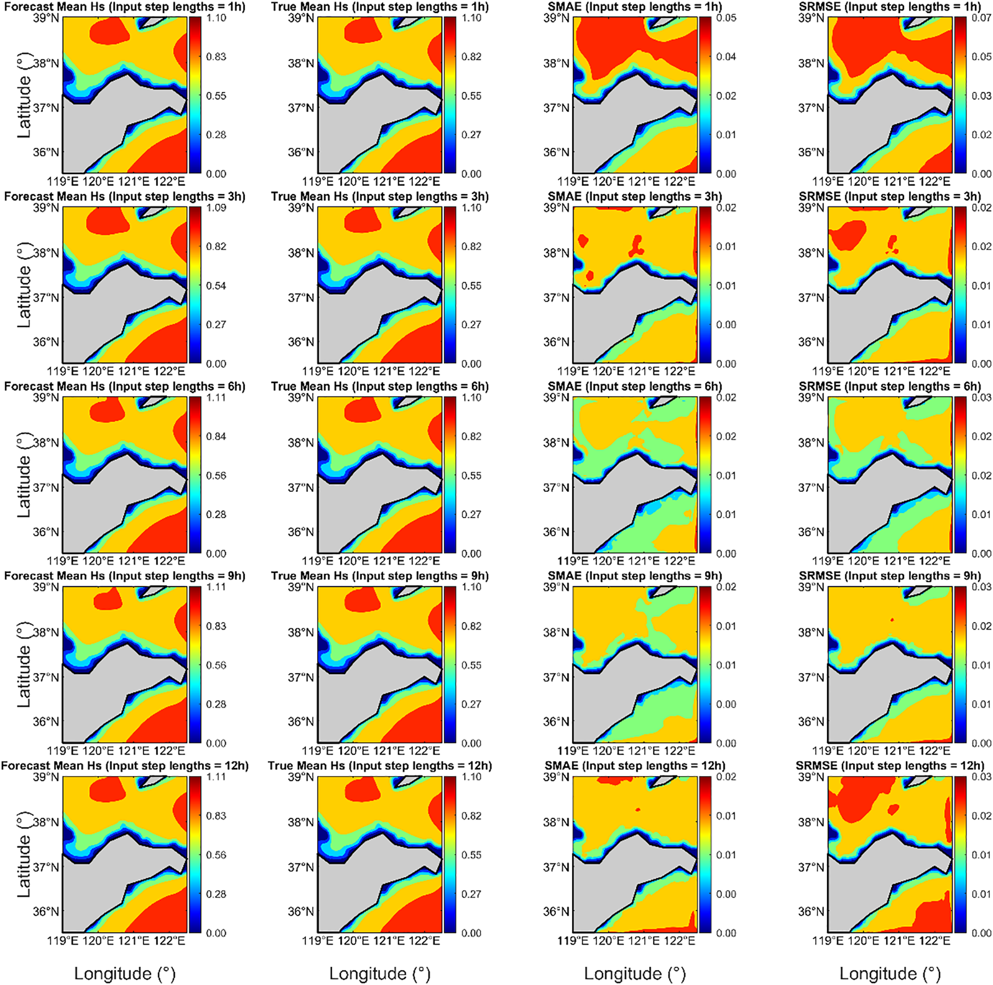
Forecasted mean Hs, True Mean Hs, SMAE, and SRMSE for a forecast lead time of 1h under different input step lengths.
Figure 8
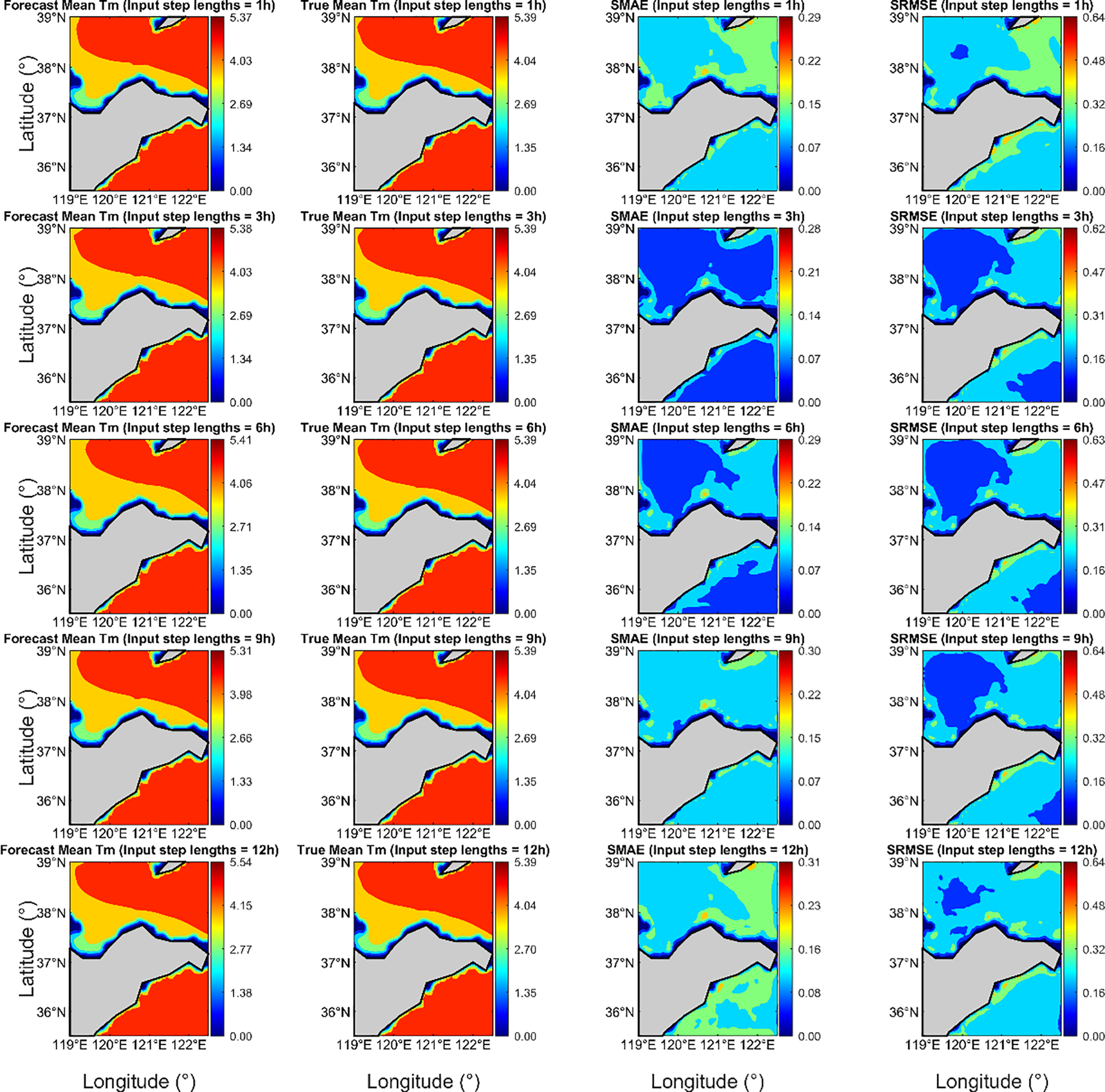
Forecasted mean Tm, True Mean Tm, SMAE, and SRMSE for a forecast lead time of 1h under different input step lengths.
3.2 Baseline model
To comprehensively evaluate our method, four classical forecasting models were selected as benchmarks in this subsection. These models are among the most widely used in intelligent wave forecasting research, including LSTM, GRU, ConvLSTM, and U-net. All models underwent hyperparameter tuning using a random search algorithm, with the search space settings detailed in Table 5 of Section 3.2. The tuning involved parameters such as the number of hidden layers, number of neurons, optimizer, and learning rate, with the optimal hyperparameters shown in Table 7. Among them, the “Neurons per layer” parameter in LSTM and GRU models represents the number of neurons in each hidden layer of LSTM and GRU layers; the “Neurons per layer” in the U-Net model corresponds to the number of convolutional kernels in the convolutional layers at each stage of the encoder. The “Neurons per layer” in the ConvLSTM model represents the number of convolutional kernels in each ConvLSTM layer. All models were configured with an input sequence length of 3 h of historical wave data to generate 1 hour ahead forecasts. The error metrics results are presented in Table 8, which demonstrates that our model exhibits certain advantages in predicting both Hs and Tm, with lower RMSE and MAE values compared to other baseline models. This indicates its enhanced capability to capture key features of Hs and Tm. Therefore, subsequent chapters will focus on wave forecasting at different time points based on this model.
Table 7
| Baseline models | Hyper-parameters | Hs model | Tm model |
|---|---|---|---|
| LSTM | Number of hidden layers | 4 | 2 |
| Neurons per layer | [288, 48, 320, 128] | [352, 368] | |
| Optimizer | adam | adam | |
| Learning_rate | 0.0005 | 0.0008 | |
| GRU | Number of hidden layers | 2 | 4 |
| Neurons per layer | [224, 464] | [368, 176, 16, 64] | |
| Optimizer | adam | adam | |
| Learning_rate | 0.0003 | 0.0006 | |
| U-net | Number of encode | 3 | 3 |
| Neurons per layer | [128, 32, 256] | [32, 64, 128] | |
| Optimizer | RMSProp | RMSProp | |
| Learning_rate | 0.0004 | 0.0001 | |
| ConvLSTM | Number of hidden layers | 3 | 3 |
| Neurons per layer | [48, 176, 240] | [80, 144, 256] | |
| Optimizer | adam | adam | |
| Learning_rate | 0.0001 | 0.0003 |
Optimal hyperparameters for different baseline models.
Table 8
| Model | Ours | LSTM | GRU | U-net | ConvLSTM |
|---|---|---|---|---|---|
| Hs’s CC | 0.9997 | 0.9942 | 0.9973 | 0.9990 | 0.9995 |
| Hs’s MAE (m) | 0.0075 | 0.0278 | 0.0191 | 0.0101 | 0.0407 |
| Hs’s RMSE (m) | 0.0149 | 0.0503 | 0.0340 | 0.0229 | 0.0621 |
| Tm’s CC | 0.9969 | 0.9916 | 0.9913 | 0.9949 | 0.9968 |
| Tm’s MAE (s) | 0.0562 | 0.1473 | 0.1478 | 0.0841 | 0.0693 |
| Tm’s RMSE (s) | 0.2014 | 0.3139 | 0.3194 | 0.2452 | 0.2187 |
Comparison of forecasting performance across different wave prediction models.
3.3 Analysis of model forecasting performance at different lead time
Based on the discussion and analysis in Section 4.1, we determined that the optimal input time step for both the Hs forecasting model and the Tm forecasting model is 3 h. Accordingly, we conducted forecasts for Hs and Tm at different lead time and analyzed the trend of model error variation with respect to time changes based on error metrics.
Table 9 summarizes the error metrics for Hs and Tm forecasts at input step length 3 h for forecast lead time of 3h, 6h, 9h, and 12h. For Hs forecasting, as the forecast lead time increases, the CC decreases from 0.9945 to 0.8757, with the rate of decline accelerating; the MAE increases from 0.0342 m to 0.1784 m, and the RMSE increases from 0.0661 m to 0.3039 m, with both showing an initial rapid increase followed by a slower rise. For Tm forecasting, the CC decreases from 0.9885 to 0.9492, with the rate of decline gradually slowing; the MAE increases from 0.1582 s to 0.4845 s, and the RMSE increases from 0.3831 s to 0.8072 s, with both showing an initial rapid increase followed by a slower rise. It can be observed that as the forecast lead time increases, the error metrics for both Hs and Tm forecasts deteriorate, with accuracy gradually decreasing. However, except for the CC in Hs forecasting, the rate of change in other error metrics gradually slows, indicating that the model’s forecasting performance becomes increasingly stable, with a certain ability to suppress error accumulation, maintaining a relatively controlled error growth trend as the forecast lead time increases.
Table 9
| Forecast horizon | 1 h | 3 h | 6 h | 9 h | 12 h |
|---|---|---|---|---|---|
| Hs’s CC | 0.9997 | 0.9945 | 0.9680 | 0.9241 | 0.8757 |
| Hs’s MAE (m) | 0.0075 | 0.0342 | 0.0919 | 0.1321 | 0.1784 |
| Hs’s RMSE (m) | 0.0149 | 0.0661 | 0.1614 | 0.2380 | 0.3039 |
| Tm’s CC | 0.9969 | 0.9885 | 0.9744 | 0.9625 | 0.9492 |
| Tm’s MAE (s) | 0.0562 | 0.1582 | 0.3243 | 0.3934 | 0.4845 |
| Tm’s RMSE (s) | 0.2014 | 0.3831 | 0.5918 | 0.6901 | 0.8072 |
Analysis of CNN model forecasting performance at different lead time.
Bold values indicate optimal performance.
Figures 9 , 10 illustrate the distribution of forecasted mean values, true mean values, SMAE, and SRMSE for the Hs and Tm models across different forecast lead times in the study area. It can be observed that the forecasted mean Hs and true mean Hs are primarily distributed between 0.6 m and 0.8 m, while the forecasted mean Tm and true mean Tm are mainly distributed between 3 s and 4 s. As the forecast lead time increases, the SMAE and SRMSE values continuously increase, but the rate of increase gradually slows, further confirming that the model’s forecasting performance becomes increasingly stable. In terms of spatial distribution, the error distribution of the Hs model is relatively regular, with smaller values near the coast and increasing values with greater offshore distance. This indicates that Hs variations in nearshore areas are highly predictable, with better model performance, while offshore areas are influenced by complex hydrodynamic processes, leading to reduced model accuracy and larger errors. For the Tm model, larger deviations are observed at certain nearshore points and in the northeastern part of the study area, suggesting that nearshore regions are affected by complex physical processes such as topography and water depth variations, resulting in more pronounced dynamic changes in Tm. The model fails to fully capture these local effects, leading to increased prediction errors. The spatial distribution of errors further underscores the significant role of local environmental factors in wave forecasting. This indicates that future research needs to incorporate complex ocean currents, variations in seabed topography, and wind interactions into the model considerations to enhance forecast accuracy under complex marine conditions.
Figure 9
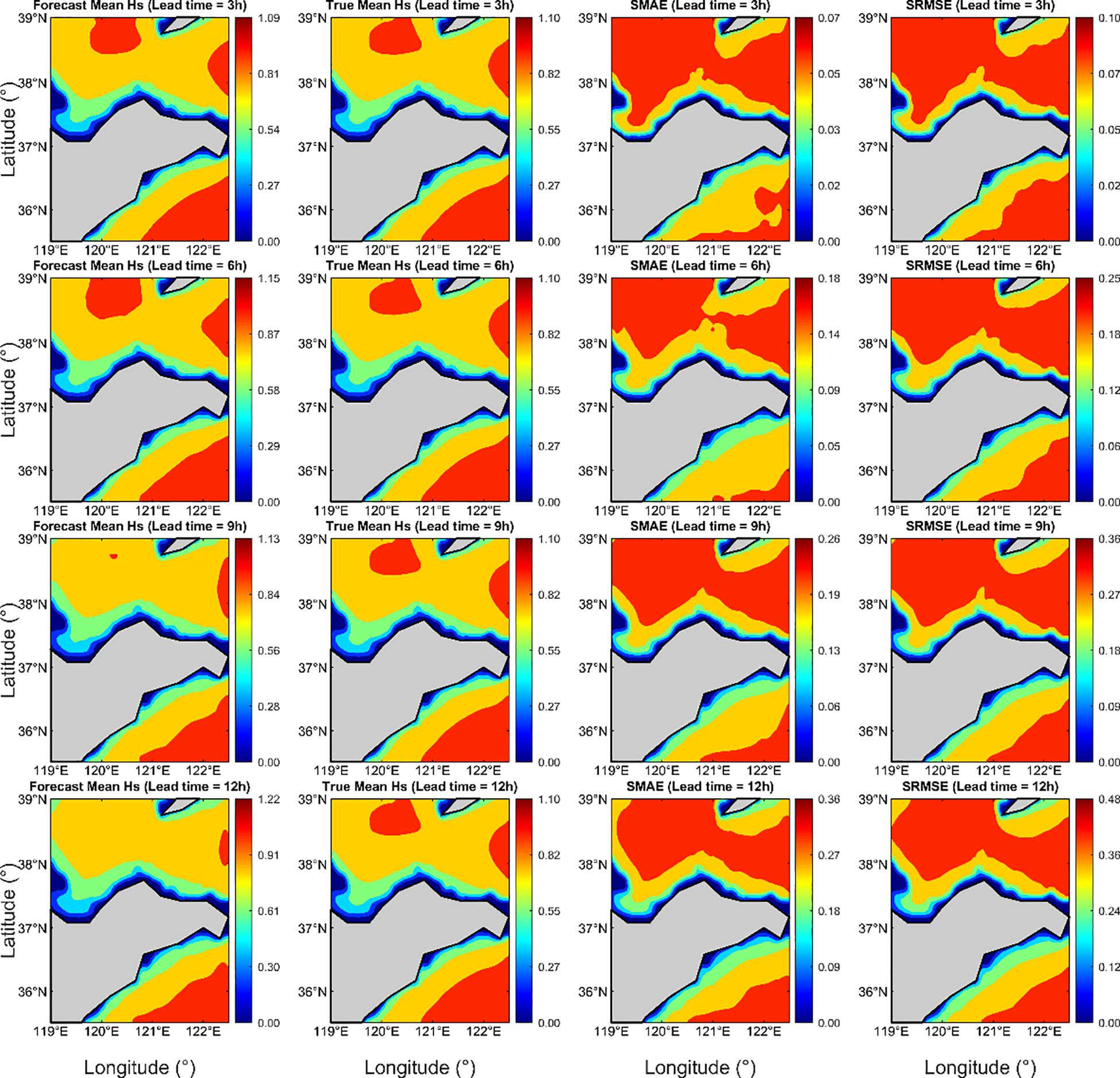
Forecast mean Hs, True mean Hs, SMAE, and SRMSE at different forecast lead times.
Figure 10
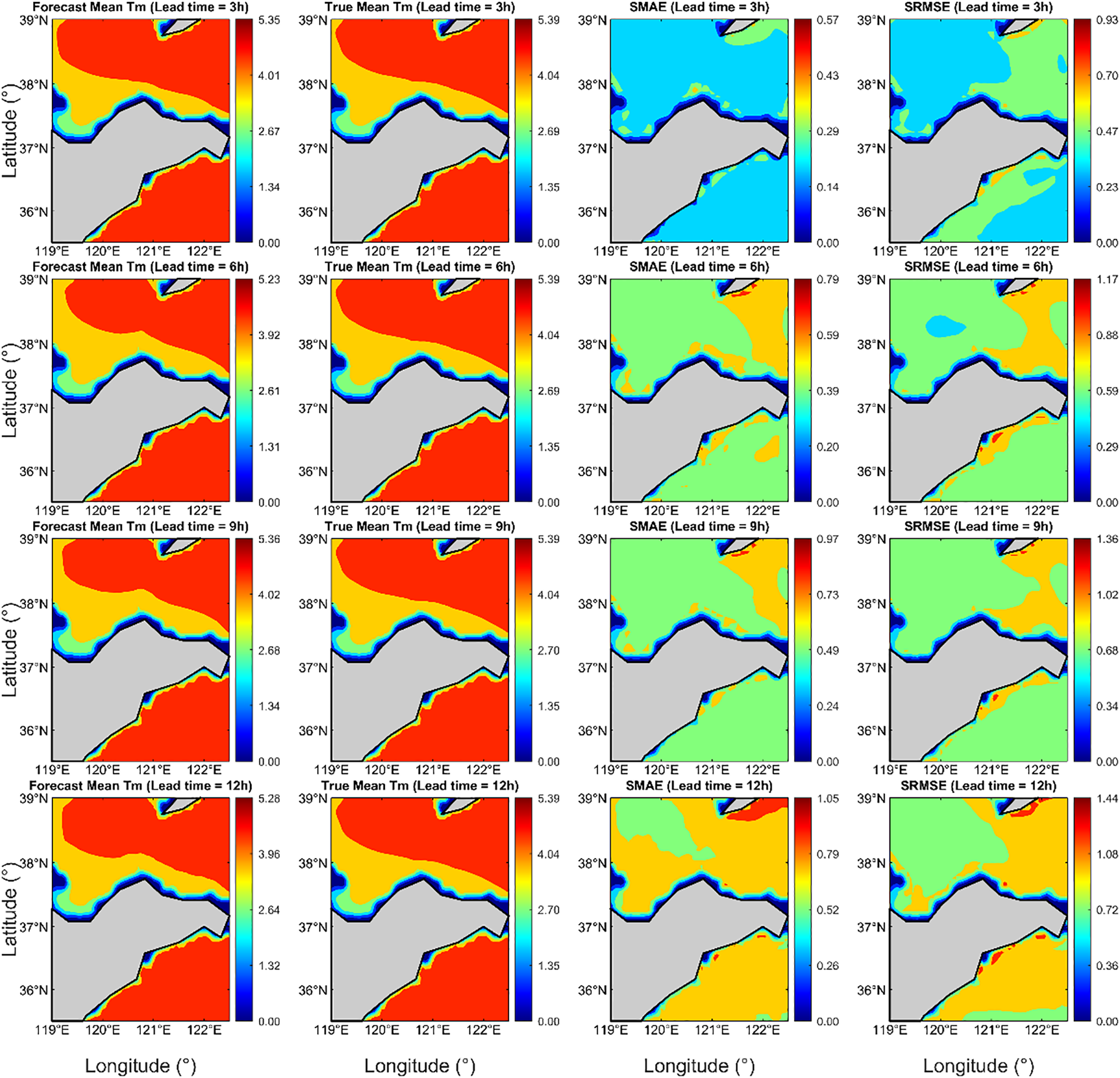
Forecast mean Tm, True mean Tm, SMAE, and SRMSE at different forecast lead times.
Figure 11 illustrates the time series of forecasted and true values of Hs and Tm, averaged over the two-dimensional spatial domain, for different forecast lead times. The left column shows the comparison for Hs, and the right column for Tm, visually demonstrating the degree of fit between forecasted and true values. It can be observed that at forecast lead times of 3 hours and 6 hours, the forecasted curves closely align with the true curves in terms of trend, with minimal phase differences. The timing and amplitude of peaks and troughs are largely consistent, indicating the model’s strong performance in capturing short-term wave dynamics. As the forecast lead time increases, a phase lag between forecasted and true values becomes more apparent, with the timing of forecasted peaks and troughs slightly delayed compared to the true values. This indicates a decline in the model’s forecasting accuracy and reflects certain limitations in capturing long-term temporal dependencies. However, the overall trend continues to effectively reflect the long-term variations in wave dynamics. In general, the model successfully captures the main trends of Hs and Tm across different forecast lead times, providing valuable scientific support for the safety and efficiency of marine operations in the fishing zone, effectively enhancing fishery production efficiency, and optimizing fishing operation scheduling.
Figure 11
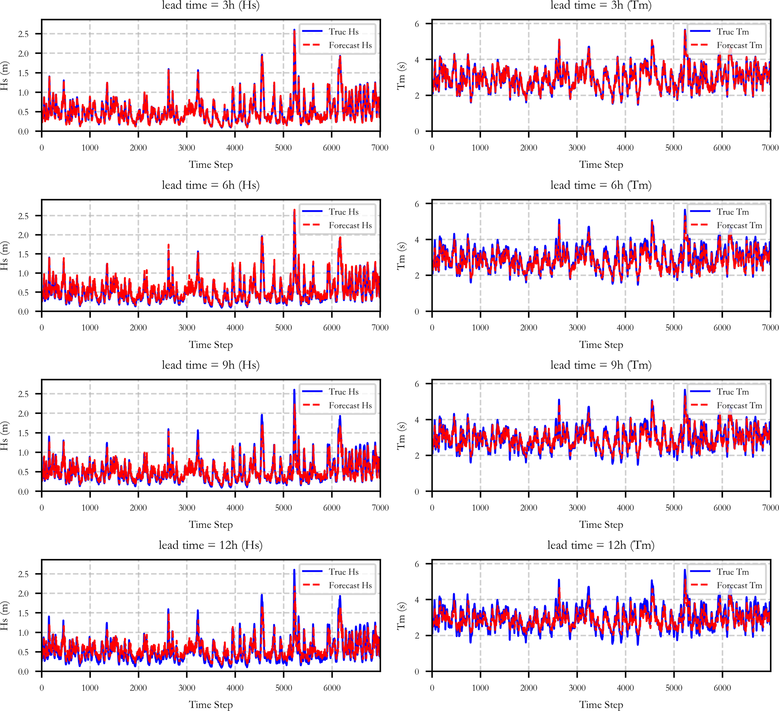
Time series plot of forecasted Hs and true Hs (left) and time series plot of forecasted Tm and true Tm (right).
4 Discussion
This study proposes an intelligent forecasting model for Hs and Tm. By utilizing the SWAN model as the data source and constructing a CNN model optimized through random search for hyperparameter tuning, the proposed approach achieves rapid forecasting of high spatiotemporal resolution Hs and Tm in the Yantai Fishing Zone, China. The SWAN model is used to generate high spatiotemporal resolution datasets, while the CNN model, leveraging local connectivity and weight-sharing mechanisms, utilizes convolutional layers to quickly capture critical wave information and learn the spatiotemporal variation characteristics of waves. Through multi-layer feature extraction, the model effectively simulates the nonlinear evolution patterns of complex wave fields.
We designed multiple experiments and determined through error analysis that the optimal input step length for the model is 3 h. Based on this optimal input step length, forecasts and analyses were conducted for different lead times. Using the SWAN dataset from 2021 to 2024, we constructed separate forecasting models for Hs and Tm. According to the error statistics, when the model’s input step length is 3 h, the CC for Hs and Tm under a 1-hour forecast are 0.9997 and 0.9969, respectively, with MAE of 0.0075 m and 0.0562 s, and RMSE of 0.0149 m and 0.2014 s. The SMAE are concentrated between 0.006 m~0.01 m for Hs and 0.05 s~0.10 s for Tm, while the SRMSE are concentrated between 0.01 m~0.02 m for Hs and 0.1 s~0.2 s for Tm. The forecasting performance is superior to other input step lengths. Although the performance differences are small, the positive impact of the input step length on the model gradually increases as the forecast lead time extends. Subsequently, we conducted forecasts for Hs and Tm over different lead times. As the forecast lead time increased, the CC gradually decreased, while the MAE, RMSE, SMAE, and SRMSE gradually increased. However, the rate of increase slowed down, indicating a decline in model’s forecast accuracy and a certain degree of lag. The model tended to underestimate Hs and Tm, particularly at peak and trough values. Nevertheless, it effectively captured the main trends in Hs and Tm changes, demonstrating the model’s good applicability. Overall, our model can accurately forecast the trends of Hs and Tm, produce high-quality forecast results, and effectively estimate the spatial distribution of Hs and Tm. Compared to traditional numerical models, the computational efficiency is significantly improved, reducing the time required to generate one-year of wave forecast data from approximately 12 hours on a 36-core server to just 20 seconds, providing an efficient and reliable solution for real-time forecasting in complex marine environments.
The current research method relies solely on Hs and Tm as inputs. It should be noted that since waves in the study area are primarily wind-driven (Huiru et al., 2017), the wind field serves as the direct driving force for wave formation. Dynamic changes in wind speed and direction significantly influence the generation, development, and dissipation of waves, particularly during sudden strong wind events or abrupt shifts in wind direction. Due to the neglect of the spatiotemporal influence of the wind field, the model often fails to accurately capture the rapid response of waves, leading to underestimation in extreme value forecasts. Additionally, local topographic variations and ocean currents also play important roles in wave propagation and evolution. Complex topographic features tend to induce complicated physical phenomena such as wave refraction, reflection, and breaking, which alter wave propagation paths and increase energy dissipation. This affects the spatial distribution of the wave field and local intensity variations, reduces the model’s ability to capture spatiotemporal characteristics of waves, and consequently leads to decreased predictive accuracy in complex marine areas. Wave-current interactions modify wave speed and wavelength, thereby influencing wave distribution characteristics and impairing the model’s ability to reflect the evolution of waves in real marine environments, resulting in reduced accuracy of model predictions. The absence of these factors somewhat diminishes the model’s predictive precision and physical interpretability, limiting its applicability under extreme weather conditions and in complex marine areas.
5 Conclusions
This study develops a CNN-based intelligent wave forecasting model using the SWAN model as the data source. Optimized through random search, the model achieves rapid and accurate prediction of high spatiotemporal resolution Hs and Tm in the Yantai Fishing Zone. The model demonstrates excellent performance in short-term forecasting and significantly outperforms traditional numerical methods in computational efficiency, meeting the requirements for near real-time prediction. It effectively captures the main wave trends and spatial distribution but exhibits partial underestimation in extreme value predictions, which limits improvements in forecast accuracy and generalization capability. In future research, incorporating wind field factors, high-resolution topographic data, and ocean current data as input features is expected to enhance the model’s predictive accuracy and mitigate error accumulation over extended forecast periods. Furthermore, integrating modeling approaches such as Physics-Informed Neural Networks (PINNs), which incorporate prior physical constraints, can improve the physical interpretability of wave prediction models, thereby enhancing their real-time applicability in marine environments.
Statements
Data availability statement
The raw data supporting the conclusions of this article will be made available by the authors, without undue reservation.
Author contributions
LZ: Conceptualization, Writing – review & editing, Methodology, Funding acquisition, Validation, Software, Writing – original draft. QL: Validation, Visualization, Writing – review & editing, Funding acquisition, Software, Investigation, Writing – original draft. XH: Visualization, Project administration, Data curation, Writing – original draft, Investigation. CH: Writing – review & editing, Supervision, Project administration, Investigation, Visualization. FJ: Writing – review & editing, Validation, Investigation, Supervision, Data curation. SW: Project administration, Investigation, Writing – review & editing, Methodology, Supervision. JY: Validation, Writing – review & editing, Investigation, Visualization, Data curation. JC: Investigation, Data curation, Resources, Writing – review & editing, Validation. MW: Resources, Writing – review & editing, Supervision, Investigation, Visualization. XM: Visualization, Formal Analysis, Data curation, Investigation, Writing – review & editing.
Funding
The author(s) declared that financial support was received for this work and/or its publication. This research was supported by Hainan Tropical Ocean University Yazhou Bay Innovation Institute Key Research and Development Project (2025CXYZDYF01), the project “Research and Demonstration Application of a Fishery Area and Fishing Port Forecasting System Based on High-Resolution Wave Numerical Simulation” funded by the China Oceanic Development Foundation, Three-Year Action Plan of North China Sea Bureau, Ministry of Natural Resources for Empowering High-Quality Marine Development through Scientific and Technological Innovation(Grant No. 2023B18-YJC), the Natural Science Foundation of Shandong Province (Grant No. ZR2024QD277) and the National Natural Science Foundation of China (42377457).
Conflict of interest
The author(s) declared that this work was conducted in the absence of any commercial or financial relationships that could be construed as a potential conflict of interest.
Generative AI statement
The author(s) declared that generative AI was not used in the creation of this manuscript.
Any alternative text (alt text) provided alongside figures in this article has been generated by Frontiers with the support of artificial intelligence and reasonable efforts have been made to ensure accuracy, including review by the authors wherever possible. If you identify any issues, please contact us.
Publisher’s note
All claims expressed in this article are solely those of the authors and do not necessarily represent those of their affiliated organizations, or those of the publisher, the editors and the reviewers. Any product that may be evaluated in this article, or claim that may be made by its manufacturer, is not guaranteed or endorsed by the publisher.
References
1
Ali F. A. Kai K. H. Khamis S. A. (2024). Assessing the variability of extreme weather events and its influence on marine accidents along the northern coast of Tanzania. Am. J. Climate Change13, 499–521. doi: 10.4236/ajcc.2024.133023
2
Alves J. H. G. Banner M. L. (2003). Performance of a saturation-based dissipation-rate source term in modeling the fetch-limited evolution of wind waves. J. Phys. Oceanogr.33, 1274–1298. doi: 10.1175/1520-0485(2003)033<1274:POASDS>2.0.CO;2
3
Bai G. Wang Z. Zhu X. Feng Y. (2022). Development of a 2-D deep learning regional wave field forecast model based on convolutional neural network and the application in South China Sea. Appl. Ocean Res.118, 103012. doi: 10.1016/j.apor.2021.103012
4
Bergstra J. Bengio Y. (2012). Random search for hyper-parameter optimization. J. Mach. Learn. Res.13, 281–305. doi: 10.5555/2188385.2188395
5
Bischl B. Binder M. Lang M. Pielok T. Richter J. Coors S. et al . (2023). Hyperparameter optimization: Foundations, algorithms, best practices, and open challenges. Wiley Interdiscip. Reviews: Data Min. Knowledge Discov.13, e1484. doi: 10.48550/arXiv.2107.05847
6
Booij N. Ris R. C. Holthuijsen L. H. (1999). A third-generation wave model for coastal regions 1. Model description and validation. J. Geophys. Res.: Oceans104, 7649–7666. doi: 10.1029/98JC02622
7
Chen J. Li S. Zhu J. Liu M. Li R. Cui X. et al . (2025). Significant wave height prediction based on variational mode decomposition and dual network model. Ocean Eng.323, 120533. doi: 10.1016/j.oceaneng.2025.120533
8
Chen J. Pillai A. C. Johanning L. Ashton I. (2021). Using machine learning to derive spatial wave data: A case study for a marine energy site. Environ. Model. Softw.142, 105066. doi: 10.1016/j.envsoft.2021.105066
9
Deka P. C. Prahlada R. (2012). Discrete wavelet neural network approach in significant wave height forecasting for multistep lead time. Ocean Eng.43, 32–42. doi: 10.1016/j.oceaneng.2012.01.017
10
Ding J. Deng F. Liu Q. Wang J. (2023). Regional forecasting of significant wave height and mean wave period using EOF-EEMD-SCINet hybrid model. Appl. Ocean Res.136, 103582. doi: 10.1016/j.apor.2023.103582
11
Fang J. Liu W. Yang S. Brown S. Nicholls R. J. Hinkel J. et al . (2017). Spatial-temporal changes of coastal and marine disasters risks and impacts in Mainland China. Ocean Coast. Manag.139, 125–140. doi: 10.1016/j.ocecoaman.2017.02.003
12
Gao Z. Liu X. Yv F. Wang J. Xing C. (2023). Learning wave fields evolution in North West Pacific with deep neural networks. Appl. Ocean Res.130, 103393. doi: 10.1016/j.apor.2022.103393
13
Group T. W. (1988). The WAM model—A third generation ocean wave prediction model. J. Phys. Oceanogr.18, 1775–1810. doi: 10.1175/1520-0485(1988)018<1775:TWMTGO>2.0.CO;2
14
Hadsell R. Sermanet P. Ben J. Erkan A. Scoffier M. Kavukcuoglu K. et al . (2009). Learning long-range vision for autonomous off-road driving. J. Field Robot.26, 120–144. doi: 10.1002/rob.20276
15
Halicki A. Dudkowska A. Gic-Grusza G. (2025). Short-term wave forecasting for offshore wind energy in the Baltic Sea. Ocean Eng.315, 119700. doi: 10.1016/j.oceaneng.2024.119700
16
Hao W. Sun X. Wang C. Chen H. Huang L. (2022). A hybrid EMD-LSTM model for non-stationary wave prediction in offshore China. Ocean Eng.246, 110566. doi: 10.1016/j.oceaneng.2022.110566
17
Hasselmann K. Barnett T. P. Bouws E. Carlson H. Cartwright D. E. Enke K. et al . (1973). Measurements of wind-wave growth and swell decay during the Joint North Sea Wave Project (JONSWAP). Ergaenzungsheft zur Deutschen Hydrographischen Zeitschrift Reihe A.
18
Huang W. Dong S. (2021). Improved short-term prediction of significant wave height by decomposing deterministic and stochastic components. Renewable Energy177, 743–758. doi: 10.1016/j.renene.2021.06.008
19
Huang X. Tang J. Shen Y. (2024a). An AI model for predicting the spatiotemporal evolution process of coastal waves by using the Improved-STID algorithm. Ocean Eng.301, 117572. doi: 10.1016/j.oceaneng.2024.117572
20
Huang X. Tang J. Shen Y. Zhang C . (2024b). An AI model for predicting the spatiotemporal evolution process of coastal waves by using the Improved-STID algorithm. Appl. Ocean Res.153, 104299. doi: 10.1016/j.apor.2024.104299
21
Huiru R. Guosheng L. Linlin C. Yue Z. Ninglei O. (2017). Simulating wave climate fluctuation in the Bohai Sea related to oscillations in the East Asian circulation over a sixty year period. J. Coast. Res.33, 829–838. doi: 10.2112/JCOASTRES-D-15-00209.1
22
Jörges C. Berkenbrink C. Gottschalk H. Stumpe B. (2023). Spatial ocean wave height prediction with CNN mixed-data deep neural networks using random field simulated bathymetry. Ocean Eng.271, 113699. doi: 10.1016/j.oceaneng.2023.113699
23
LeCun Y B. Y. H. G. (2015). Deep learning. Nature521, 436–444. doi: 10.1038/nature14539
24
Li G. Zhang H. Lyu T. Zhang H. (2024). Regional significant wave height forecast in the East China Sea based on the Self-Attention ConvLSTM with SWAN model. Ocean Eng.312, 119064. doi: 10.1016/j.oceaneng.2024.119064
25
Liu Y. Lu W. Wang D. Lai Z. Ying C. Li X. et al . (2024). Spatiotemporal wave forecast with transformer-based network: A case study for the northwestern Pacific Ocean. Ocean Model.188, 102323. doi: 10.1016/j.ocemod.2024.102323
26
Mandal S. Prabaharan N. (2006). Ocean wave forecasting using recurrent neural networks. Ocean Eng.33, 1401–1410. doi: 10.1016/j.oceaneng.2005.08.007
27
Meng F. Song T. Xu D. Xie P. Li Y. (2021). Forecasting tropical cyclones wave height using bidirectional gated recurrent unit. Ocean Eng.234, 108795. doi: 10.1016/j.oceaneng.2021.108795
28
Ning F. Delhomme D. LeCun Y. Piano F. Bottou L. Barbano P. E. (2005). Toward automatic phenotyping of developing embryos from videos. IEEE Trans. Image Processing14, 1360–1371. doi: 10.1109/TIP.2005.852470
29
Oh J. Suh K. D. (2018). Real-time forecasting of wave heights using EOF–wavelet–neural network hybrid model. Ocean Eng.150, 48–59. doi: 10.1016/j.oceaneng.2017.12.044
30
Qiu D. Cheng Y. Wang X. (2023). Medical image super-resolution reconstruction algorithms based on deep learning: A survey. Comput. Methods Programs Biomed.238, 107590. doi: 10.1016/j.cmpb.2023.107590
31
Scala P. Manno G. Ingrassia E. Ciraolo G. (2025). Combining Conv-LSTM and wind-wave data for enhanced sea wave forecasting in the Mediterranean Sea. Ocean Eng.326, 120917. doi: 10.1016/j.oceaneng.2025.120917
32
Sharma A. K. Nandal A. Dhaka A. Alhudhaif A. Polat K. Sharma A. (2025). Diagnosis of cervical cancer using CNN deep learning model with transfer learning approaches. Biomed. Signal Process. Control105, 107639. doi: 10.1016/j.bspc.2025.107639
33
Taigman Y. Yang M. Ranzato M. A. Wolf L. (2014). “ Deepface: Closing the gap to human-level performance in face verification,” in Proceedings of the IEEE conference on computer vision and pattern recognition, 1701–1708.
34
Tolman H. L. Balasubramaniyan B. Burroughs L. D. Chalikov D. V. Chao Y. Y. Chen H. S. et al . (2002). Development and implementation of wind generated ocean surface models at NCEP. Weather Forecast.17, 311–333. doi: 10.1175/1520-0434(2002)017<0311:DAIOWG>2.0.CO;2
35
Tolman H. L. Chalikov D. (1996). Source terms in a third-generation wind wave model. J. Phys. Oceanogr.26, 2497–2518. doi: 10.1175/1520-0485(1996)026<2497:STIATG>2.0.CO;2
36
Tsai C. P. Lin C. Shen J. N. (2002). Neural network for wave forecasting among multi-stations. Ocean Eng.29, 1683–1695. doi: 10.1016/S0029-8018(01)00112-3
37
van der Westhuysen A. J. Zijlema M. Battjes J. A. (2007). Nonlinear saturation-based whitecapping dissipation in SWAN for deep and shallow water. Coast. Eng.54, 151–170. doi: 10.1016/j.coastaleng.2006.08.006
38
Xia H. Wang K. (2024). PreciDBPN: A customized deep learning approach for hourly precipitation downscaling in eastern China. Atmospheric Res.311, 107705. doi: 10.1016/j.atmosres.2024.107705
39
Yu M. Wang Z. Song D. Zhu Z. Pan R. (2024). Spatio-temporal ocean wave conditions forecasting using MA-TrajGRU model in the South China sea. Ocean Eng.291, 116486. doi: 10.1016/j.oceaneng.2023.116486
40
Zhang W. Sun Y. Wu Y. Dong J. Song X. Gao Z. et al . (2024). A deep-learning real-time bias correction method for significant wave height forecasts in the Western North Pacific. Ocean Model.187, 102289. doi: 10.1016/j.ocemod.2023.102289
41
Zheng Z. Ali M. Jamei M. Xiang Y. Abdulla S. Yaseen Z. M. et al . (2023). Multivariate data decomposition based deep learning approach to forecast one-day ahead significant wave height for ocean energy generation. Renewable Sustain. Energy Rev.185, 113645. doi: 10.1016/j.rser.2023.113645
42
Zhou S. Xie W. Lu Y. Wang Y. Zhou Y. Hui N. et al . (2021). ConvLSTM-based wave forecasts in the South and East China seas. Front. Mar. Science.8, 680079. doi: 10.3389/fmars.2021.680079
43
Zijlema M. Van Vledder G. P. Holthuijsen L. H. (2012). Bottom friction and wind drag for wave models. Coast. Eng.65, 19–26. doi: 10.1016/j.coastaleng.2012.03.002
44
Zilong T. Yubing S. Xiaowei D. (2022). Spatial-temporal wave height forecast using deep learning and public reanalysis dataset. Appl. Energy326, 120027. doi: 10.1016/j.apenergy.2022.120027
45
Zuo R. Xiong Y. Wang J. (2019). Deep learning and its application in geochemical mapping. Earth-science Rev.192, 1–14. doi: 10.1016/j.earscirev.2019.02.023
Summary
Keywords
ocean wave forecasting, convolutional neural network, input step lengths, short-term wave forecasting, Yantai Fishing Zone
Citation
Zhou L, Li Q, Hong X, Hou C, Jiang F, Wu S, Yan J, Cheng J, Wang M and Mao X (2025) Ocean wave conditions forecasting using convolutional neural networks in the Yantai Fishing Zone, China. Front. Mar. Sci. 12:1741623. doi: 10.3389/fmars.2025.1741623
Received
07 November 2025
Revised
24 November 2025
Accepted
28 November 2025
Published
12 December 2025
Volume
12 - 2025
Edited by
Zhenjun Zheng, Hainan University, China
Reviewed by
Xinyu Huang, Dalian University of Technology, China
Kun Liu, Shandong University, China
Updates
Copyright
© 2025 Zhou, Li, Hong, Hou, Jiang, Wu, Yan, Cheng, Wang and Mao.
This is an open-access article distributed under the terms of the Creative Commons Attribution License (CC BY). The use, distribution or reproduction in other forums is permitted, provided the original author(s) and the copyright owner(s) are credited and that the original publication in this journal is cited, in accordance with accepted academic practice. No use, distribution or reproduction is permitted which does not comply with these terms.
*Correspondence: Feifei Jiang, jff@stu.ouc.edu.cn
†These authors have contributed equally to this work
Disclaimer
All claims expressed in this article are solely those of the authors and do not necessarily represent those of their affiliated organizations, or those of the publisher, the editors and the reviewers. Any product that may be evaluated in this article or claim that may be made by its manufacturer is not guaranteed or endorsed by the publisher.